Limitations of the heavy-baryon expansion as revealed by a pion-mass dispersion relation

Abstract

The chiral expansion of nucleon properties such as mass, magnetic moment, and magnetic polarizability are investigated in the framework of chiral perturbation theory, with and without the heavy-baryon expansion. The analysis makes use of a pion-mass dispersion relation, which is shown to hold in both frameworks. The dispersion relation allows an ultraviolet cutoff to be implemented without compromising the symmetries. After renormalization, the leading-order heavy-baryon loops demonstrate a stronger dependence on the cutoff scale, which results in weakened convergence of the expansion. This conclusion is tested against the recent results of lattice QCD simulations for nucleon mass and isovector magnetic moment. In the case of the polarizability, the situation is even more dramatic as the heavy-baryon expansion is unable to reproduce large soft contributions to this quantity. Clearly, the heavy-baryon expansion is not suitable for every quantity.

I Introduction

The dependence of hadron properties on the quark masses — the chiral behavior — is crucial for interpreting the modern lattice QCD calculations, which usually require an extrapolation in the quark mass. It is also important for determining the quark mass values, as well as for any quantitative description of chiral symmetry breaking. Chiral perturbation theory ($\chi$PT) Weinberg (1979); Gasser and Leutwyler (1984), a low-energy effective field theory (EFT) of QCD, should in principle describe the nonanalytic dependencies on the light-quark masses in a systematic fashion. The analytic (series-like) dependencies are more arbitrary in $\chi$PT, and are specified in terms of low-energy constants (LECs). They are to be fixed by matching to the underlying theory, which is usually achieved by fitting to lattice QCD results.

In the baryon sector of $\chi$PT one often invokes an additional expansion in the inverse baryon masses called the heavy-baryon expansion, or HB$\chi$PT Jenkins and Manohar (1991); Bernard et al. (1995). The baryon $\chi$PT without the heavy-baryon expansion will be referred to as B$\chi$PT. While both expansions should converge to the same result, the question is whether they converge in a natural way (cf. Georgi (1991, 1993) for an explanation of ‘natural’). If the difference between them at any finite order is as crucial as is claimed, it is clear that they cannot both converge naturally. Therefore, the goal is to establish which of HB- or B$\chi$PT has the more natural expansion.

Up to a given chiral order, the B$\chi$PT result can be written as the HB$\chi$PT result and a series of contributions, which are nominally of higher order in HB$\chi$PT. Whether these contributions are indeed of smaller size can only be checked in explicit calculations, and many cases it has been observed that the difference between a given-order of HB- and B$\chi$PT results is unnaturally large Becher and Leutwyler (1999); Fuchs et al. (2003); Pascalutsa et al. (2004); Holstein et al. (2005); Pascalutsa and Vanderhaeghen (2005); Geng et al. (2008); Ledwig et al. (2012); Alarcon et al. (2011). A notable example is provided by the magnetic polarizability of the proton, for which the leading chiral-loop contribution predicts $-1.8$ in B$\chi$PT Bernard et al. (1991) or $+1.3$ in HB$\chi$PT Bernard et al. (1995), in units of $10^{-4}$ fm³. These large differences are reconciled in practice by adopting unnaturally large values for some of the LECs, appearing at higher orders in HB$\chi$PT (see e.g. Hildebrandt et al. (2004)). This is not a solution of course, but rather a restatement of the problem.

In this work, the problem is investigated by using the recently established pion-mass dispersion relation Pascalutsa (2009); Ledwig et al. (2010):

$$f(m_{\pi}^{2})=-\frac{1}{\pi}\!\int\limits_{-\infty}^{0}\!\mathrm{d}t\,\frac{\mathrm{Im}\,f(t)}{t-m_{\pi}^{2}}\,,$$ (1)

where the static quantity $f$ is a complex function of the pion mass squared $m_{\pi}^{2}$. Throughout this work, the focus is on the following static properties of the nucleon: the mass $f\equiv M_{N}$, anomalous magnetic moment (AMM) $f\equiv\kappa_{N}$, and magnetic polarizability $f\equiv\beta_{N}$. The dispersion relation results from the observation that chiral loops in $\chi$PT are analytic functions in the entire complex plane of $m_{\pi}^{2}$ except for the negative real-axis, which contains a branch cut associated with pion production, see Fig. 1.

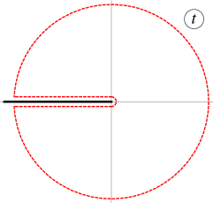
Figure 1: (color online). The complex $t=m_{\pi}^{2}$ plane, with the branch-cut along the negative real axis, and the contour indicating the analyticity domain.

As will be demonstrated in Sec. II, there is a correspondence between integrating over $t$ in the above dispersion relation and the integration over the momentum in a chiral loop. One can cut off the $t$-integration without danger of compromising the symmetries of the theory. Thus an ultraviolet cutoff $\Lambda$ is introduced in Sec. III. After subtracting positive powers of $\Lambda$ into the available LECs, the aim is to determine the scales at which differences between the HB- and B$\chi$PT appear. It is observed that cutting off the dispersion relation is equivalent to the ‘sharp cutoff’ version of finite-range regularization (FRR), introduced originally to improve the HB$\chi$PT expansion by resumming the chiral series through the introduction of a regulator into the loop integrals, see Donoghue et al. (1999); Leinweber et al. (1999); Young et al. (2002, 2003); Borasoy et al. (2002); Leinweber et al. (2004); Bernard et al. (2004); Young et al. (2005); Leinweber et al. (2005a, b). The equivalence between the cutoff dispersion relation and FRR readily allows for an extension of the FRR to the realm of B$\chi$PT.

In Sec. IV, the HB- and B$\chi$PT FRR formulae for the cases of the nucleon mass, AMMs, and magnetic polarizability are obtained at order $p^{3}$, and their residual cutoff-dependence is studied. In Sec. V, these formulae are confronted with experimental and lattice QCD results. The recent lattice QCD simulations of PACS-CS Aoki et al. (2009) and JLQCD Ohki et al. (2008) Collaborations are used for the nucleon mass, and simulations from QCDSF Collins et al. (2011) Collaboration are used for the AMMs. The conclusions are presented in Sec. VI. In the Appendix, the dispersion relation in the quark mass is considered briefly, and a condition for its ‘subtractions’ is discussed.

II Integration over loop momentum vs. pion mass

Consider the example of the nucleon mass, which, takes the following simple form to order $p^{3}$ in HB$\chi$PT:

$$M_{N}=\,\stackrel{{\scriptstyle\circ}}{{M}}_{N}-\,4\stackrel{{\scriptstyle\circ}}{{c}}_{1}\!m_{\pi}^{2}+\chi_{N}m_{\pi}^{3}.$$ (2)

$\stackrel{{\scriptstyle\circ}}{{M}}_{N}$ and $\stackrel{{\scriptstyle\circ}}{{c}}_{1}$ are the LECs to this order, and the coefficient of the nonanalytic term is given by:

$$\chi_{N}=-\frac{3g_{A}^{2}}{32\pi f_{\pi}^{2}},$$ (3)

for the empirical values of $g_{A}\simeq 1.27$ and $f_{\pi}\simeq 92.4$ MeV. The nonanalytic term follows from the self-energy graph in Fig. 2, which yields the familiar form in HB$\chi$PT:

$$\Sigma_{N}^{\mathrm{HB}}(m_{\pi}^{2})=\chi_{N}\frac{2}{\pi}\int\limits_{0}^{\infty}\mathrm{d}k\,\frac{k^{4}}{k^{2}+m_{\pi}^{2}},$$ (4)

where $k$ is the magnitude of the 3-momentum running in the loop. After a change of integration variable to $\,t=-k^{2}$, one obtains:

$$\Sigma_{N}^{\mathrm{HB}}(m_{\pi}^{2})=-\frac{1}{\pi}\!\int\limits_{-\infty}^{0}\!\mathrm{d}t\,\frac{\chi_{N}(-t)^{3/2}}{t-m_{\pi}^{2}}.$$ (5)

which is simply the pion-mass dispersion relation of Eq. (1), with: $\,\mathrm{Im}\,\Sigma_{N}^{\mathrm{HB}}(t)=\chi_{N}\,(-t)^{3/2}$. Thus it is not only evident that the heavy-baryon loop obeys the pion-mass dispersion relation, but also that there is a correspondence between the integration over the pion mass and the loop momentum. It can easily be seen that cutting off the loop momentum at some scale $\Lambda$ is equivalent to placing the lower-limit of integration over $t$ at $-\Lambda^{2}$.

Figure 2: The pion loop contribution to the self-energy of the nucleon, providing the leading nonanalytic contribution to the nucleon mass. All charge conserving transitions are implicit.

Having observed this equivalence, the dispersion relation will be used in preference to the loop integrals themselves. The reason for this is twofold. Firstly, in order to express the loop integral with only a single $k$-integration, the $k_{0}$ and angular integrations must be evaluated, which is usually more difficult than finding the imaginary part of the loop (especially for multi-loop graphs and B$\chi$PT expressions). Secondly, it is explicitly clear that no symmetries of the theory are compromised in the cutoff of $t$. Of course, it has been shown that FRR schemes with a sharp cutoff in the momentum are consistent with chiral symmetry Bernard et al. (2004). However, in $t$-integration, consistency with the symmetries is more explicit, and violations of analyticity become apparent immediately.

The cutoff-dependence of a given quantity is meaningful only after the loop contributions have been renormalized. When using the dispersion relation, the usual procedure of dimensional regularization and cancellation of infinities by counter-terms is replaced by ‘subtractions’. For instance, the nucleon mass requires at least two subtractions at $m_{\pi}^{2}=0$ (cf. Appendix A), so that the third-order contribution can be written as:

$$M_{N}^{(3)}=-\frac{1}{\pi}\!\int\limits_{-\infty}^{0}\!\mathrm{d}t\,\frac{\mathrm{Im}\,M_{N}^{(3)}(t)}{t-m_{\pi}^{2}}\,\frac{m_{\pi}^{4}}{t^{2}}\stackrel{{\scriptstyle\mathrm{HB}}}{{=}}\chi_{N}\,m_{\pi}^{3},$$ (6)

with the full result, to order $p^{3}$, given by Eq. (2). The LECs play the role of the subtraction constants.

Introduction of an ultraviolet cutoff in the finite integral after the subtractions allows one to separate the low- and high-momentum contributions. It can also provide information about the scale at which the HB- and B$\chi$PT results start to deviate.

III Introducing a cutoff: finite-range regularization

The chiral expansion of an observable quantity $f$ is an expansion in the quark mass $m_{q}$ around the chiral limit ($m_{q}~{}\to~{}0$), which in $\chi$PT becomes an expansion in $p=m_{\pi}/\Lambda_{\chi}$, the mass of the pseudo-Goldstone boson of spontaneous chiral symmetry breaking over the scale of chiral symmetry breaking $\Lambda_{\chi}\simeq 4\pi f_{\pi}\approx 1$ GeV Manohar and Georgi (1984). Because of the branch cut in the complex-$m_{\pi}^{2}$ plane along the negative real-axis, the chiral expansion is not a series expansion (otherwise, it would have a zero radius of convergence), but rather an expansion in non-integer powers of $m_{\pi}^{2}\propto m_{q}$.

By writing the dispersion integral as:

$$f(m_{\pi}^{2})=-\frac{1}{\pi}\left(\,\int\limits_{-\Lambda_{\chi}^{2}}^{0}+\int\limits_{-\infty}^{-\Lambda_{\chi}^{2}}\,\right)\mathrm{d}t\,\frac{\mathrm{Im}\,f(t)}{t-m_{\pi}^{2}},$$ (7)

it is evident that the second integral can be expanded in integer powers of $m_{\pi}^{2}/\Lambda_{\chi}^{2}$. Hence this term is of analytic form and can only affect the values of the LECs. Indeed, the physics above the scale $\Lambda_{\chi}$ is not described by $\chi$PT and therefore its effect should be absorbable by the LECs.

The second integral generates an infinite number of analytic terms, while the number of LECs to a given order of the calculation is finite. The higher-order analytic terms are present and not compensated by the LECs at this order, but their effect should not exceed the uncertainty in the calculation due to the neglect of all the other higher-order terms. That is, the second integral can be dropped, while the resulting cutoff-dependence represents the uncertainty due to higher-order effects.

One purpose of imposing a cutoff of order of $1$ GeV is to investigate the convergence of the expansion without actually computing any of the higher-order contributions. This is one the main goals of FRR– indeed, motivated by the absence of rapid curvature in all hadronic observables at larger quark masses, FRR aims to resum the chiral expansion in the expectation of improving the convergence of the residual series Young et al. (2003); Leinweber et al. (2004); Leinweber et al. (2005b); Hall et al. (2010, 2011). From the formulae shown in Eqs. (4) – (6) in the previous section, it is clear that the ‘sharp cutoff’ FRR is equivalent to the cutoff pion-mass dispersion relation:

$$f(m_{\pi}^{2};\Lambda^{2})=-\frac{1}{\pi}\!\int\limits_{-\Lambda^{2}}^{0}\!\!\mathrm{d}t\,\frac{\mathrm{Im}\,f(t)}{t-m_{\pi}^{2}}\left(\frac{m_{\pi}^{2}}{t}\right)^{n},$$ (8)

where $n$ indicates the number of subtractions around the chiral limit. In this work, the main aim is to see at which values of the cutoff any deviation occurs between the HB- and B$\chi$PT results. If the deviation begins at $\Lambda\ll 1$ GeV, then the differences between the two expansions cannot be reconciled in a natural way. In the next section, this situation is examined using several specific examples, and for each of them a different picture is obtained (cf. Fig. 3).

IV Nucleon properties at $\mathcal{O}(p^{3})$

At chiral order $p^{3}$, the imaginary parts of the nucleon mass, the proton and neutron AMMs, and the magnetic polarizability of the proton were computed in Ref. Ledwig et al. (2010):

$$\mathrm{Im}\,M_{N}^{(3)}(t) =\frac{3g_{A}^{2}\hat{M}_{N}^{3}}{(4\pi f_{\pi})^{2}}\frac{\pi\tau}{2}\Big{(}\frac{1}{2}\tau+\lambda\Big{)}\,\theta(-t)\,,$$ (9a)

$$\mathrm{Im}\,\kappa_{p}^{(3)}(t) =\frac{g_{A}^{2}\hat{M}_{N}^{2}}{(4\pi f_{\pi})^{2}}\frac{2\pi}{\lambda}\Big{(}\frac{1}{2}\tau+\lambda\Big{)}^{2}\Big{[}1-\frac{3}{2}\Big{(}\frac{1}{2}\tau+\lambda\Big{)}\Big{]}$$

$$\qquad\times\,\theta(-t)\,,$$ (9b)

$$\mathrm{Im}\,\kappa_{n}^{(3)}(t) =-\frac{g_{A}^{2}\hat{M}_{N}^{2}}{(4\pi f_{\pi})^{2}}\frac{2\pi}{\lambda}\Big{(}\frac{1}{2}\tau+\lambda\Big{)}^{2}\,\theta(-t)\,,$$ (9c)

$$\mathrm{Im}\,\beta^{(3)}_{p}(t) =-\frac{(e^{2}/4\pi)\,g_{A}^{2}}{(4\pi f_{\pi})^{2}\hat{M}_{N}}\frac{\pi\tau}{24\lambda^{3}}\Big{[}2-72\lambda$$

$$+(418\lambda-246)\,\tau-(316\lambda-471)\,\tau^{2}$$

$$+(54\lambda-212)\,\tau^{3}+27\tau^{4}\Big{]}\,\theta(-t),$$ (9d)

where $\hat{M}_{N}\simeq 939$ MeV is the physical nucleon mass, $e^{2}/4\pi\simeq 1/137$ is the fine-structure constant, and the following dimensionless variables are introduced:

$$\tau=\frac{t}{\hat{M}_{N}^{2}},\quad\lambda=\sqrt{\frac{1}{4}\tau^{2}-\tau}\,.$$ (10)

The expression for the mass comes from the graph in Fig. 2, with leading (pseudo-vector) $\pi NN$ coupling. The expressions for the AMMs and polarizability come from graphs obtained from Fig. 2 by minimal insertion(s) of $1$- and $2$-photons, respectively.

The corresponding heavy-baryon expressions at order $p^{3}$ can be obtained by keeping only the leading in $1/\hat{M}_{N}$ term (i.e, $\lambda\approx\sqrt{-\tau}$, etc.):

$$\mathrm{Im}\,M_{N}^{(3)}(t) \stackrel{{\scriptstyle\mathrm{HB}}}{{=}}\frac{3g_{A}^{2}\hat{M}_{N}^{3}}{(4\pi f_{\pi})^{2}}\frac{\pi\tau}{2}\sqrt{-\tau}\,\theta(-t)\,,$$ (11a)

$$\mathrm{Im}\,\kappa_{p}^{(3)}(t) \stackrel{{\scriptstyle\mathrm{HB}}}{{=}}\frac{g_{A}^{2}\hat{M}_{N}^{2}}{(4\pi f_{\pi})^{2}}\,2\pi\sqrt{-\tau}\,\theta(-t)\stackrel{{\scriptstyle\mathrm{HB}}}{{=}}-\,\mathrm{Im}\,\kappa_{n}^{(3)}(t),$$ (11b)

$$\mathrm{Im}\,\beta^{(3)}_{p}(t) \stackrel{{\scriptstyle\mathrm{HB}}}{{=}}\frac{(e^{2}/4\pi)\,g_{A}^{2}}{(4\pi f_{\pi})^{2}\hat{M}_{N}}\frac{\pi}{12\sqrt{-\tau}}\,\theta(-t).$$ (11c)

The full, renormalized result for a given quantity is obtained by substituting these imaginary parts into the dispersion relation of Eq. (8). The number of subtractions required in each case differ: $n=2$ for $M_{N}$, $n=1$ for AMMs, and no subtractions for polarizability. The resulting expressions read as follows:

$$M_{N}(m_{\pi}^{2};\Lambda^{2}) = \,\stackrel{{\scriptstyle\circ}}{{M}}_{N}\!-\,4\stackrel{{\scriptstyle\circ}}{{c}}_{1}\!m_{\pi}^{2}-\frac{\chi_{N}}{\pi}\!\!\!\int\limits_{-\Lambda^{2}}^{0}\!\!\mathrm{d}t\frac{\Big{[}(-t)^{3/2}\sqrt{1-\frac{t}{4\hat{M}_{N}^{2}}}-\frac{t^{2}}{2\hat{M}_{N}}\Big{]}}{t-m_{\pi}^{2}}\left(\frac{m_{\pi}^{2}}{t}\right)^{2}$$ (12a)

$$= \,\stackrel{{\scriptstyle\circ}}{{M}}_{N}\!-\,4\stackrel{{\scriptstyle\circ}}{{c}}_{1}\!m_{\pi}^{2}+\frac{\chi_{N}m_{\pi}^{4}}{2\pi\hat{M}_{N}}\Bigg{\{}2\sqrt{\frac{4\hat{M}_{N}^{2}}{m_{\pi}^{2}}-1}\,\arctan\Bigg{(}\frac{\Lambda}{m_{\pi}}\sqrt{\frac{4\hat{M}_{N}^{2}-m_{\pi}^{2}}{4\hat{M}_{N}^{2}+\Lambda^{2}}}\Bigg{)}$$

$$+\,2\,\mathrm{arcsinh}\frac{\Lambda}{2\hat{M}_{N}}+\log\frac{m_{\pi}^{2}}{m_{\pi}^{2}+\Lambda^{2}}\Bigg{\}},$$

$$\kappa_{p}(m_{\pi}^{2};\Lambda^{2}) = \stackrel{{\scriptstyle\circ}}{{\kappa}}_{p}+\,\frac{g_{A}^{2}\hat{M}_{N}^{2}}{(4\pi f_{\pi})^{2}}\bigg{\{}\frac{m_{\pi}(-8+22\mbox{$\frac{m_{\pi}^{2}}{\hat{M}_{N}^{2}}$}-6\mbox{$\frac{m_{\pi}^{4}}{\hat{M}_{N}^{4}}$})}{\hat{M}_{N}\Big{(}4-\mbox{$\frac{m_{\pi}^{2}}{\hat{M}_{N}^{2}}$}\Big{)}^{1/2}}\,\arctan\Bigg{(}\frac{\Lambda}{m_{\pi}}\sqrt{\frac{4\hat{M}_{N}^{2}-m_{\pi}^{2}}{4\hat{M}_{N}^{2}+\Lambda^{2}}}\Bigg{)}$$ (12b)

$$- \frac{m_{\pi}^{2}}{\hat{M}_{N}^{2}}\Big{(}5-\frac{3m_{\pi}^{2}}{\hat{M}_{N}^{2}}\Big{)}\,\left[2\,\mathrm{arcsinh}\frac{\Lambda}{2\hat{M}_{N}}+\log\frac{m_{\pi}^{2}}{m_{\pi}^{2}+\Lambda^{2}}\right]+\frac{3m_{\pi}^{2}\Lambda^{2}}{\hat{M}_{N}^{4}}\left(1-\sqrt{1+\frac{4\hat{M}_{N}^{2}}{\Lambda^{2}}}\,\right)\bigg{\}},$$

$$\kappa_{n}(m_{\pi}^{2};\Lambda^{2}) = \stackrel{{\scriptstyle\circ}}{{\kappa}}_{n}+\,\frac{4g_{A}^{2}\hat{M}_{N}^{2}}{(4\pi f_{\pi})^{2}}\bigg{\{}\frac{m_{\pi}(2-\mbox{$\frac{m_{\pi}^{2}}{\hat{M}_{N}^{2}}$})}{\hat{M}_{N}\Big{(}4-\mbox{$\frac{m_{\pi}^{2}}{\hat{M}_{N}^{2}}$}\Big{)}^{1/2}}\,\arctan\Bigg{(}\frac{\Lambda}{m_{\pi}}\sqrt{\frac{4\hat{M}_{N}^{2}-m_{\pi}^{2}}{4\hat{M}_{N}^{2}+\Lambda^{2}}}\Bigg{)}$$ (12c)

$$+ \frac{m_{\pi}^{2}}{2\hat{M}_{N}^{2}}\left[2\,\mathrm{arcsinh}\frac{\Lambda}{2\hat{M}_{N}}+\log\frac{m_{\pi}^{2}}{m_{\pi}^{2}+\Lambda^{2}}\right]\bigg{\}},$$

$$\beta_{p}(m_{\pi}^{2};\Lambda^{2}) = \frac{(e^{2}/4\pi)\,g_{A}^{2}}{3(4\pi f_{\pi})^{2}}\Bigg{\{}\,\frac{2(2-246\mbox{$\frac{m_{\pi}^{2}}{\hat{M}_{N}^{2}}$}+471\mbox{$\frac{m_{\pi}^{4}}{\hat{M}_{N}^{4}}$}-212\mbox{$\frac{m_{\pi}^{6}}{\hat{M}_{N}^{6}}$}+27\mbox{$\frac{m_{\pi}^{8}}{\hat{M}_{N}^{8}}$})}{m_{\pi}\Big{(}4-\mbox{$\frac{m_{\pi}^{2}}{\hat{M}_{N}^{2}}$}\Big{)}^{3/2}}\,\arctan\Bigg{(}\frac{\Lambda}{m_{\pi}}\sqrt{\frac{4\hat{M}_{N}^{2}-m_{\pi}^{2}}{4\hat{M}_{N}^{2}+\Lambda^{2}}}\Bigg{)}$$

$$- \Big{(}\frac{9}{\hat{M}_{N}}-\frac{50m_{\pi}^{2}}{\hat{M}_{N}^{3}}+\frac{27m_{\pi}^{4}}{\hat{M}_{N}^{5}}\Big{)}\,\left[2\,\mathrm{arcsinh}\frac{\Lambda}{2\hat{M}_{N}}+\log\frac{m_{\pi}^{2}}{m_{\pi}^{2}+\Lambda^{2}}\right]$$

$$- \frac{\Lambda^{2}}{\hat{M}_{N}^{3}}\left[\frac{27(\Lambda^{2}-2m_{\pi}^{2})}{2\hat{M}_{N}^{2}}\left(1-\sqrt{1+\frac{4\hat{M}_{N}^{2}}{\Lambda^{2}}}\,\right)+50-23\sqrt{1+\frac{4\hat{M}_{N}^{2}}{\Lambda^{2}}}-\frac{51\hat{M}_{N}^{6}}{\Lambda^{2}(4\hat{M}_{N}^{2}+\Lambda^{2})(4\hat{M}_{N}^{2}-m_{\pi}^{2})}\right]\Bigg{\}}\,.$$

The heavy-baryon expressions can be obtained by picking out the leading in $1/\hat{M}_{N}$ term, or equivalently, by substituting the corresponding imaginary parts from Eq. (11), into the dispersion relation. In the latter case, the same integral is encountered in all of the examples:

$$J(m_{\pi};\Lambda)\equiv\int\limits_{-\Lambda^{2}}^{0}\!\mathrm{d}t\,\frac{1}{(t-m_{\pi}^{2})\sqrt{-t}}=-\frac{2}{m_{\pi}}\arctan\frac{\Lambda}{m_{\pi}}.$$ (13)

All of the above quantities to $\mathcal{O}(p^{3})$ in HB$\chi$PT are given by this integral, up to an overall constant, and a factor of $m_{\pi}^{2n}$. $n$ is the number of subtractions (or pertinent LECs) at this order.

In Fig. 3, the resulting cutoff-dependence of the above loop contributions is shown at the physical value of the pion mass: $m_{\pi}\simeq 139$ MeV. Each quantity (mass, isovector AMM, and polarizability) is presented in a separate panel, where the results with and without the heavy-baryon expansion are displayed.

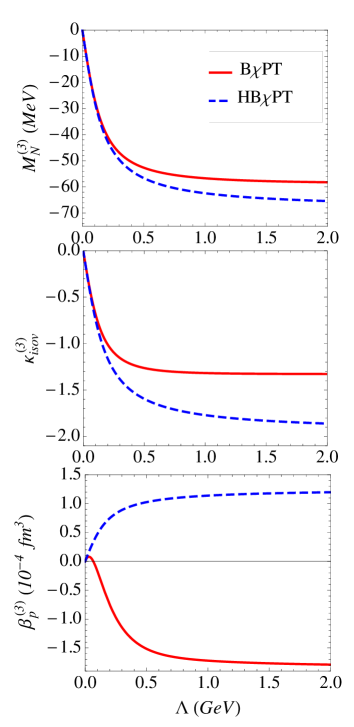
Figure 3: (color online). The cutoff-dependence of leading-order loop contributions to various nucleon quantities (mass, isovector AMM, and proton’s magnetic polarizability) calculated in HB$\chi$PT (blue dashed curves) and B$\chi$PT (red solid curves).

This figure illustrates the following two features:

1. As seen from Eqs. (12) and (13), the residual cutoff-dependence in HB$\chi$PT falls off as $1/\Lambda$ in all of the considered examples, while the dependence in the case of B$\chi$PT behaves as $1/\Lambda^{2}$ for $M_{N}$, and as $1/\Lambda^{4}$ for both AMMs and $\beta_{p}$ despite the presence of the positive powers of $\Lambda$ in Eqs. (12b – d). The HB$\chi$PT results have a stronger cutoff-dependence than the B$\chi$PT results, indicating a larger impact of the unknown high-energy physics to be renormalized by higher-order LECs. Hence, the HB results are at bigger risk of producing a large contribution from the high-momentum region. Note that, although not necessarily immediately apparent from Fig. 3, the cutoff-dependence of the relativistically improved chiral formulae can be obtained from Eqs. (12a – d), and in the heavy-baryon case, from the chiral formulae from the FRR literature; e.g. see Refs. Leinweber et al. (2005b); Young et al. (2005).

2. The HB- and B$\chi$PT results are guaranteed to be the same at small values of $\Lambda$ (and not only at $\Lambda=0$), as can be seen by taking derivatives of Eq. (8) with respect to $\Lambda^{2}$, at $\Lambda=0$. However, at finite values of $\Lambda$ the differences are appreciable. Observing significant differences for $\Lambda$ of order $m_{\pi}$, as in the case of $\beta_{p}$, indicates that the size of the $1/\hat{M}_{N}$ terms is largely underestimated in HB$\chi$PT.

V Matching: confronting lattice results

Eventually, the $\chi$PT results must be matched to the underlying theory – or in practice – fitted to experimental and lattice QCD simulation results. In this section, it will be demonstrated that chiral extrapolations based on the relativistic expressions of Eqs. (12a – d) are more stable with respect to cutoff variation.

The case of magnetic polarizability is interesting. Since there are no unknown LECs at leading order, it constitutes a genuine prediction. Unfortunately, there are no lattice results for this quantity, while the experimental data are largely uncertain (see Ref. Lensky and Pascalutsa (2010) for a recent discussion). One thing that the data indisputably show is that $\beta_{p}$ is small compared to the electric polarizability, and positive, which seems to be more consistent with the HB$\chi$PT result. However, it is well known that $\beta_{p}$ must have a large positive contribution from the excitation of the $\Delta(1232)$ resonance Lensky and Pascalutsa (2010), which can only be accommodated if the chiral loops are negative and partially cancel it out.

For the nucleon mass, one does not expect much difference between HB- and B$\chi$PT around the physical pion mass, based on Fig. 3. For larger pion masses, however, the difference becomes significant, and may affect the fit to lattice results as is shown in what follows.

In Figs. 4 and 5, chiral extrapolations of recent lattice results from PACS-CS Aoki et al. (2009) and JLQCD Ohki et al. (2008) are presented. The different panels correspond to different values of the cutoff $\Lambda$, while the dashed and solid curves correspond to HB- and B$\chi$PT fit at order $p^{3}$. The values of the fit parameters obtained using PACS-CS and JLQCD results are shown in Tables 1 and 2, respectively.

The PACS-CS results were generated using non-perturbatively $\mathcal{O}(a)$-improved Wilson quark action at a lattice box size of $\sim 2.9$ fm, but the set only contains five points, and there is a large statistical error in the smallest $m_{\pi}^{2}$ point. The JLQCD results were generated using overlap fermions in $N_{f}=2$ QCD. The lattice box length for each simulation result is $\sim 1.9$ fm, with a corresponding lattice spacing is $0.118$ fm. The box size is small compared to that of the PACS-CS simulations, but the statistical uncertainties in each point are also smaller. For simplicity, the fits also neglect possible finite-volume corrections.

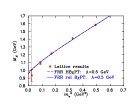
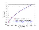
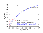
Figure 4: (color online). Comparison of chiral extrapolations of the nucleon mass for HB$\chi$PT (black dashed curves) compared to the relativistic formula of B$\chi$PT (blue solid curves) from Eq. (12a), at various values of sharp-cutoff scale of $\Lambda$. The extrapolation based on PACS-CS results Aoki et al. (2009), box size: $2.9$ fm.

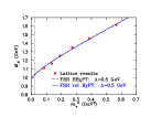
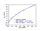
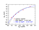
Figure 5: (color online). Comparison of chiral extrapolations of the nucleon mass for HB$\chi$PT (black dashed curves) compared to the relativistic formula of B$\chi$PT (blue solid curves) from Eq. (12a), at various values of sharp-cutoff scale of $\Lambda$. The extrapolation based on JLQCD results Ohki et al. (2008), box size: $1.9$ fm.

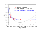
Figure 6: (color online). Comparison of chiral extrapolations of the anomalous magnetic moment for HB$\chi$PT (black dashed curves) compared to the relativistic formula of B$\chi$PT (blue solid curves), for three different values of $\Lambda$. The extrapolation based on QCDSF results Collins et al. (2011), box size: $1.7-2.9$ fm.

Previous studies in HB$\chi$PT have indicated that, for lattice results extending outside the chiral power-counting regime, the optimal value of the FRR scale $\Lambda$ is of the order $\Lambda\approx 1$ GeV Hall et al. (2010). Clearly, Fig. 4 shows agreement that the best heavy-baryon result is obtained for $\Lambda\approx 1$ GeV. The heavy-baryon extrapolation is much more sensitive to changes in the FRR scale $\Lambda$ compared with the B$\chi$PT extrapolation, in agreement with Fig. 3.

For small values of $\Lambda$, the HB$\chi$PT and B$\chi$PT results are similar, since the chiral loops are suppressed. An almost-linear fit eventuates in both cases. This is not ideal, as Fig. 4 indicates that neglecting the chiral curvature leads to a poor fit of the low-energy lattice results. For larger values of $\Lambda$, the heavy-baryon extrapolation struggles to fit the lattice results due to large curvature in the heavy pion-mass region. The relativistic extrapolation appears to produce a more stable fit to the lattice results across a range of values of cutoff scale $\Lambda$.

The importance of accommodating chiral curvature is even greater in the case of observables with lower-order leading nonanalytic terms in their chiral expansions, such as the magnetic moment of the nucleon. In the case of the AMMs, recent lattice QCD simulations by the QCDSF collaboration are used Collins et al. (2011).

The results from QCDSF were generated using $N_{f}=2$ and the $\mathcal{O}(a)$-improved Wilson quark action, with box sizes ranging from $1.7$ to $2.9$ fm. To ensure that the lattice results from QCDSF give a reasonable approximation to the infinite volume limit, the following restrictions are applied: $L>1.5$ fm and $m_{\pi}L>3$. There are nine lattice points that satisfy these criteria from the original set of results. Additionally, the isovector combination of the nucleon ($p-n$) is used in lattice QCD to avoid calculating the disconnected loops that occur in full QCD, which are computationally intensive, since they involve the calculation of all-to-all propagators. In general, diagrams contributing to the AMM of a hadron include photons coupling to sea-quark loops. In the special case of the isovector, the diagrams that include these disconnected loops cancel.

Table 1: A comparison of the values of the fit parameters $\stackrel{{\scriptstyle\circ}}{{M}}_{N}$ and $\stackrel{{\scriptstyle\circ}}{{c}}_{1}$ for HB$\chi$PT and relativistic B$\chi$PT for various values of regularization scale $\Lambda$, based on lattice results from PACS-CS.

$\Lambda$(GeV)	$\stackrel{{\scriptstyle\circ}}{{M}}_{N}^{\mathrm{HB}}$(GeV)	$\stackrel{{\scriptstyle\circ}}{{M}}_{N}^{\mathrm{B}}$(GeV)	$\stackrel{{\scriptstyle\circ}}{{c}}_{1}^{\mathrm{HB}}$(GeV-1)	$\stackrel{{\scriptstyle\circ}}{{c}}_{1}^{\mathrm{B}}$(GeV-1)
$0.5$	$0.953$($22$)	$0.963$($22$)	$-0.709$($9$)	$-0.660$($9$)
$1.0$	$0.856$($22$)	$0.896$($22$)	$-0.970$($9$)	$-0.840$($9$)
$3.0$	$0.717$($22$)	$0.833$($22$)	$-1.278$($9$)	$-0.981$($9$)

Table 2: A comparison of the values of the fit parameters $\stackrel{{\scriptstyle\circ}}{{M}}_{N}$ and $\stackrel{{\scriptstyle\circ}}{{c}}_{1}$ for HB$\chi$PT and relativistic B$\chi$PT for various values of regularization scale $\Lambda$, based on lattice results from JLQCD.

$\Lambda$(GeV)	$\stackrel{{\scriptstyle\circ}}{{M}}_{N}^{\mathrm{HB}}$(GeV)	$\stackrel{{\scriptstyle\circ}}{{M}}_{N}^{\mathrm{B}}$(GeV)	$\stackrel{{\scriptstyle\circ}}{{c}}_{1}^{\mathrm{HB}}$(GeV-1)	$\stackrel{{\scriptstyle\circ}}{{c}}_{1}^{\mathrm{B}}$(GeV-1)
$0.5$	$0.986$($8$)	$0.997$($8$)	$-0.676$($1$)	$-0.627$($1$)
$1.0$	$0.880$($8$)	$0.924$($8$)	$-0.943$($1$)	$-0.811$($1$)
$3.0$	$0.721$($8$)	$0.851$($8$)	$-1.265$($1$)	$-0.959$($1$)

The B$\chi$PT integral results from Eqs. (12b) &  (12c) can be adapted for chiral extrapolation of the nucleon isovector by taking the difference between the proton and neutron AMM formulae. In addition, a linear term in $m_{\pi}^{2}$ is added with a free fit parameter $a_{2}$, which plays the role of compensating some of the high-momentum contributions:

$$\kappa_{\mathrm{isov}}(m_{\pi}^{2},\Lambda^{2})=\kappa_{p}(m_{\pi}^{2},\Lambda^{2})-\kappa_{n}(m_{\pi}^{2},\Lambda^{2})+a_{2}m_{\pi}^{2}.$$ (14)

Without it, the heavy-baryon result is just a straight line, and the differences between the two frameworks are irreconcilable in this range of pion masses.

The corresponding chiral behavior of the isovector nucleon AMM is shown in Fig. 6 for three different values of $\Lambda$, with corresponding values of the fit parameters shown in Table 3. Note that the curvature of the extrapolation using a sharp-cutoff regulator with $\Lambda=1.0$ GeV is already large. This is a consequence of the leading-order nonanalytic behavior of the AMM occurring at a lower chiral order ($\sim\!m_{\pi}$) than for the nucleon mass ($\sim\!m_{\pi}^{3}$). However, the extrapolation using the relativistic B$\chi$PT formulae of Eqs. (12b) & (12c) is comparatively insensitive to changes in the FRR scale $\Lambda$. This indicates that the B$\chi$PT formulae are largely independent of the ultraviolet behavior.

Table 3: A comparison of the values of the fit parameter $\stackrel{{\scriptstyle\circ}}{{\kappa}}_{\mathrm{isov}}$ and $a_{2}$ for HB$\chi$PT and relativistic B$\chi$PT for various values of regularization scale $\Lambda$.

$\Lambda$(GeV)	$\stackrel{{\scriptstyle\circ}}{{\kappa}}_{\mathrm{isov}}^{\mathrm{HB}}$	$\stackrel{{\scriptstyle\circ}}{{\kappa}}_{\mathrm{isov}}^{\mathrm{B}}$	$a_{2}^{\mathrm{HB}}$ (GeV-2)	$a_{2}^{\mathrm{B}}$ (GeV-2)
$0.5$	$5.23$($5$)	$4.13$($5$)	$0.70$($10$)	$0.14$($10$)
$0.8$	$6.27$($5$)	$4.28$($5$)	$3.42$($10$)	$0.65$($10$)
$1.0$	$6.68$($5$)	$4.31$($5$)	$5.46$($10$)	$0.83$($10$)

As shown in the previous section the naturalness problem doesn’t arise in the AMM, in the same drastic way as it does in the polarizability. However for a broader range of pion masses the problem starts to show. In the case of AMM, $a_{2}^{HB}$ quickly becomes larger with increasing $\Lambda$, in order to accommodate the large higher-momentum contributions.

VI Conclusion: when heavy-baryon fails

The HB$\chi$PT and B$\chi$PT can be viewed as two different ways of organizing the chiral EFT expansion in the baryon sector. While the heavy-baryon expansion is often considered to be more consistent from the power-counting point of view, it appears to be less natural. Certain terms that are nominally suppressed by powers of $m_{\pi}/M_{N}$, and hence dropped in HB$\chi$PT as being ‘higher order’, appear to be significant in explicit calculations.

The problem is more pronounced in some quantities and less in others. To quantify this, one needs to note the power of the expansion parameter at which the chiral loops begin to contribute to the quantity in question. For the considered examples of the nucleon mass, AMMs, and polarizability, this power index is $3$, $1$, and $-1$, respectively. The smaller the index, the greater is the difficulty for HB$\chi$PT to describe this quantity in a natural way. For quantities with a negative index, a dramatic failure of HB$\chi$PT is expected.

The negative index simply means that the chiral expansion of that quantity begins at lowest order with negative powers of $m_{\pi}$. Apart from polarizabilities, the most notable quantities of this kind are the coefficients of the effective-range expansion of the nuclear force. As is known, the non-relativistic $\chi$PT in the two-nucleon sector Kaplan et al. (1998) failed to describe these quantities Cohen and Hansen (1999), thus precluding the idea of ‘perturbative pions’ in this sector . The present work encourages one to think that B$\chi$PT can solve this problem, as is the case for nucleon polarizabilities.

It certainly is important to understand the origin of the apparent difficulty of the HB expansion in estimating quantum corrections in certain observables, at least in a way it has been understood for the scalar form factor Becher and Leutwyler (1999). Here, it was only shown that the behaviour comes from the “soft” momentum region, and a criterion for determining the region relevant to this problem was conjectured. The understanding of the origin presents a challenge for future studies.

Appendix A The quark-mass dispersion relation and subtractions

According to the Gell-Mann–Oakes–Renner relation (GOR) Gell-Mann et al. (1968), $m_{\pi}^{2}\propto m_{q}$ for a light-quark mass $m_{q}$. Thus, the pion-mass dispersion relation can be translated into a quark-mass dispersion relation (as seen in Eq. (1)):

$$f(m_{q})=-\frac{1}{\pi}\!\int\limits_{-\infty}^{0}\!\mathrm{d}t\,\frac{\mathrm{Im}f(t)}{t-m_{q}}\,,$$ (15)

with $f$ being a function of $m_{q}$. The above allusion to GOR implies that this relation is valid for small $m_{q}$ only. However, if its validity were assumed for all $m_{q}$, the issue of its convergence for a given quantity $f$ could be considered as follows.

The unsubtracted dispersion relation implies that $f~{}\propto~{}1/m_{q}$, for large $m_{q}$, which obviously cannot be true for every quantity. For example, In the case of the nucleon mass $f\equiv M_{N}$, it is expected that $f\propto m_{q}$ for large $m_{q}$. Therefore, the relation needs to be subtracted at least twice, i.e:

$$M_{N}(m_{q})=\,\stackrel{{\scriptstyle\circ}}{{M}}_{N}+\,a_{1}m_{q}-\frac{m_{q}^{2}}{\pi}\!\int\limits_{-\infty}^{0}\!\frac{\mathrm{d}t}{t^{2}}\,\frac{\mathrm{Im}\,M_{N}(t)}{t-m_{q}}\,,$$ (16)

with $\stackrel{{\scriptstyle\circ}}{{M}}_{N}$ and $a_{1}$ being the subtraction constants.

In another example, the nucleon AMM should behave a constant for large $m_{q}$ and hence one subtraction will suffice:

$$\kappa_{N}(m_{q})=\,\,\stackrel{{\scriptstyle\circ}}{{\kappa}}_{N}-\,\frac{m_{q}}{\pi}\!\int\limits_{-\infty}^{0}\!\frac{\mathrm{d}t}{t}\,\frac{\mathrm{Im}\,\kappa_{N}(t)}{t-m_{q}}\,,$$ (17)

where $\stackrel{{\scriptstyle\circ}}{{\kappa}}_{N}$ is the AMM in the chiral limit, playing the role of the subtractions constant.

The sufficiency of these subtractions is confirmed in leading-order $\chi$PT calculations. At higher chiral orders, more subtractions are needed as new low-energy constants arise to play the role of the subtraction constants. The above analysis determines only the minimal number of subtractions for a given quantity.

References

- Weinberg (1979) S. Weinberg, Physica A96, 327 (1979).
- Gasser and Leutwyler (1984) J. Gasser and H. Leutwyler, Annals Phys. 158, 142 (1984).
- Jenkins and Manohar (1991) E. E. Jenkins and A. V. Manohar, Phys. Lett. B255, 558 (1991).
- Bernard et al. (1995) V. Bernard, N. Kaiser, and U.-G. Meissner, Int.J.Mod.Phys. E4, 193 (1995), eprint hep-ph/9501384.
- Georgi (1991) H. Georgi, Nucl.Phys. B361, 339 (1991).
- Georgi (1993) H. Georgi, Ann.Rev.Nucl.Part.Sci. 43, 209 (1993).
- Becher and Leutwyler (1999) T. Becher and H. Leutwyler, Eur.Phys.J. C9, 643 (1999), eprint hep-ph/9901384.
- Fuchs et al. (2003) T. Fuchs, J. Gegelia, G. Japaridze, and S. Scherer, Phys.Rev. D68, 056005 (2003), eprint hep-ph/0302117.
- Pascalutsa et al. (2004) V. Pascalutsa, B. R. Holstein, and M. Vanderhaeghen, Phys.Lett. B600, 239 (2004), eprint hep-ph/0407313.
- Holstein et al. (2005) B. R. Holstein, V. Pascalutsa, and M. Vanderhaeghen, Phys.Rev. D72, 094014 (2005), eprint hep-ph/0507016.
- Pascalutsa and Vanderhaeghen (2005) V. Pascalutsa and M. Vanderhaeghen, Phys.Rev.Lett. 95, 232001 (2005), eprint hep-ph/0508060.
- Geng et al. (2008) L. Geng, J. Martin Camalich, L. Alvarez-Ruso, and M. Vicente Vacas, Phys. Rev. Lett. 101, 222002 (2008), eprint 0805.1419.
- Ledwig et al. (2012) T. Ledwig, J. Martin-Camalich, V. Pascalutsa, and M. Vanderhaeghen, Phys. Rev. D85, 034013 (2012), eprint 1108.2523.
- Alarcon et al. (2011) J. Alarcon, J. Martin Camalich, and J. Oller (2011), eprint 1110.3797.
- Bernard et al. (1991) V. Bernard, N. Kaiser, and U. G. Meissner, Phys. Rev. Lett. 67, 1515 (1991).
- Hildebrandt et al. (2004) R. P. Hildebrandt, H. W. Griesshammer, T. R. Hemmert, and B. Pasquini, Eur.Phys.J. A20, 293 (2004), eprint nucl-th/0307070.
- Pascalutsa (2009) V. Pascalutsa, PoS CD09, 095 (2009), eprint 0910.3686.
- Ledwig et al. (2010) T. Ledwig, V. Pascalutsa, and M. Vanderhaeghen, Phys.Lett. B690, 129 (2010), eprint 1004.3449.
- Donoghue et al. (1999) J. F. Donoghue, B. R. Holstein, and B. Borasoy, Phys. Rev. D59, 036002 (1999), eprint hep-ph/9804281.
- Leinweber et al. (1999) D. B. Leinweber, D.-H. Lu, and A. W. Thomas, Phys.Rev. D60, 034014 (1999), eprint hep-lat/9810005.
- Young et al. (2002) R. D. Young, D. B. Leinweber, A. W. Thomas, and S. V. Wright, Phys. Rev. D66, 094507 (2002), eprint hep-lat/0205017.
- Young et al. (2003) R. D. Young, D. B. Leinweber, and A. W. Thomas, Prog. Part. Nucl. Phys. 50, 399 (2003), eprint hep-lat/0212031.
- Borasoy et al. (2002) B. Borasoy, B. R. Holstein, R. Lewis, and P. P. A. Ouimet, Phys. Rev. D66, 094020 (2002), eprint hep-ph/0210092.
- Leinweber et al. (2004) D. B. Leinweber, A. W. Thomas, and R. D. Young, Phys. Rev. Lett. 92, 242002 (2004), eprint hep-lat/0302020.
- Bernard et al. (2004) V. Bernard, T. R. Hemmert, and U.-G. Meissner, Nucl. Phys. A732, 149 (2004), eprint hep-ph/0307115.
- Young et al. (2005) R. D. Young, D. B. Leinweber, and A. W. Thomas, Phys. Rev. D71, 014001 (2005), eprint hep-lat/0406001.
- Leinweber et al. (2005a) D. B. Leinweber et al., Phys. Rev. Lett. 94, 212001 (2005a), eprint hep-lat/0406002.
- Leinweber et al. (2005b) D. B. Leinweber, A. W. Thomas, and R. D. Young, Nucl.Phys. A755, 59 (2005b), eprint hep-lat/0501028.
- Aoki et al. (2009) S. Aoki et al. (PACS-CS Collaboration), Phys.Rev. D79, 034503 (2009), eprint 0807.1661.
- Ohki et al. (2008) H. Ohki et al., Phys. Rev. D78, 054502 (2008), eprint 0806.4744.
- Collins et al. (2011) S. Collins, M. Gockeler, P. Hagler, R. Horsley, Y. Nakamura, et al., Phys.Rev. D84, 074507 (2011), eprint 1106.3580.
- Manohar and Georgi (1984) A. Manohar and H. Georgi, Nucl. Phys. B234, 189 (1984).
- Hall et al. (2010) J. Hall, D. Leinweber, and R. Young, Phys.Rev. D82, 034010 (2010), eprint 1002.4924.
- Hall et al. (2011) J. Hall, F. Lee, D. Leinweber, K. Liu, N. Mathur, et al., Phys.Rev. D84, 114011 (2011), eprint 1101.4411.
- Lensky and Pascalutsa (2010) V. Lensky and V. Pascalutsa, Eur.Phys.J. C65, 195 (2010), eprint 0907.0451.
- Kaplan et al. (1998) D. B. Kaplan, M. J. Savage, and M. B. Wise, Nucl.Phys. B534, 329 (1998), eprint nucl-th/9802075.
- Cohen and Hansen (1999) T. D. Cohen and J. M. Hansen, Phys.Rev. C59, 13 (1999), eprint nucl-th/9808038.
- Epelbaum and Gegelia (2012) E. Epelbaum and J. Gegelia, Phys.Lett. B716, 338 (2012), eprint 1207.2420.
- Gell-Mann et al. (1968) M. Gell-Mann, R. Oakes, and B. Renner, Phys.Rev. 175, 2195 (1968).