A simple solvable energy landscape model that shows a thermodynamic phase transition and a glass transition

Abstract

When a liquid melt is cooled, a glass or  phase transition can be obtained depending on the cooling rate. Yet, this behavior has not been clearly captured in energy landscape models. Here a model is provided in which two key ingredients are considered based in the landscape, metastable states and their multiplicity. Metastable states are considered as in two level system models. However, their multiplicity and topology allows a phase transition in the thermodynamic limit, while a transition to the glass is obtained for fast cooling. By solving the corresponding master equation, the minimal speed of cooling required to produce the glass is obtained as a function of the distribution of metastable and stable states. This allows to understand cooling trends due to rigidity considerations in chalcogenide glasses.

Humankind has been using glassy materials since the dawn of civilization. However, their process of formation still poses many questions Anderson Relaxation Micoulaut Kerner2 Mauro1 Mauro2 Magdaleno . Glasses do not have long range order and are formed out of thermal equilibrium, resulting in a limited use of the traditional tools of the trade in solid state and statistical mechanics. Moreover, numerical simulations are not able to provide definitive answers, since cooling speeds achieved in numerical simulations are orders of magnitude higher than in real cases Debenebook . One of the main issues is the nature of the glass transition Debenedetti , for example, is it a purely dynamical effect or there is a underlying thermodynamical singularity? The answer to this question has practical implications, as how to calculate the minimal cooling speed depending on the chemical composition in order to form a glass, or why some chemical compounds form glasses while others will never reach such state Phillips1 . Concerning this relationship between chemical composition and minimal cooling speed, PhillipsPhillips1 observed that for several chalcogenides, this minimal speed is a function of rigidity. This initial observation was the ingnition spark for the extensive investigation on rigidity of glassesThorpe0 Boolchand3 Georgiev Naumis Huerta0 Huerta1 Huerta Huertaprb , yet this basic observation has not been quantitatively explained.

On the other hand, the energy landscape has been a useful picture to understand glass transition Debenedetti . However, due to its complicate high dimensional topology, it is difficult to obtain closed analytical results. It is not even clear how a phase transition is related with the topology of the landscape, i.e., why a global minimum leads to singularities in the thermodynamical behavior. Clearly, there is a lack of a minimal simple solvable model of landscape that can display a phase and a glass transition depending on the cooling rate. Here we present such model by combining the two most basic ingredients that are belived to be fundamental in the problem. Furthermore, the model allows to get a glimpse on the connection between minimal cooling speed, energy landscapes, rigidity, and Boolchand intermediate phases IBoolchand1 IBoolchand3 .

The first ingredient is based in a well known fact: glasses are trapped in metastable states, while crystals are global minimums in the landscape. A common way to describe the corresponding physics is through the use of two level system (TLS). If the glassy metastable state has energy $E_{1}$ and the crystalline global minimum an energy $E_{0}=0$, the system is trapped in the glassy state due to an energy barrier $V$ measured from $E_{1}$, as seen in Fig. 1. Following Huse et. al.Huse and Langer et. al. Langerprl Langer Langer1990 , who described the residual population of the metastable state for a TLS at zero temperature, the cooling process can be described by a master equation, in which the probabibilty $p(t)$ of finding the system in the metastable state, assuming that the system is in contact with a bath at temperature $T$, isLangerprl ,

$$\frac{dp(t)}{dt}=-\Gamma_{\uparrow\downarrow}p(t)+\Gamma_{\downarrow\uparrow}\left[1-p(t)\right],$$ (1)

where $\Gamma_{\uparrow\downarrow}$ is the transition rate from the upper well to the lower, and the transitions from the lower to the upper take place at rate $\Gamma_{\downarrow\uparrow}=e^{-\frac{E_{1}}{T}}\Gamma_{\uparrow\downarrow}$. If quantum mechanical tunneling is neglected, $\Gamma_{\uparrow\downarrow}=$ $\Gamma_{0}e^{-\frac{V}{T}}$, where $\Gamma_{0}$ is a small frequency of oscillation at the bottom of the walls.

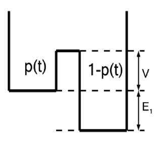
Figure 1: The two level system energy landscape, showing the barrier height $V$ and the asymmetry $E_{1}$ between the two levels. The population of the upper well is $p(t)$.

Eq. (1) describes the relaxation towards $p_{0}(T)$, the population at thermal equilibrium obtained from the stationary condition, as can be seen by rewriting Eq. (1) as Langerprl ,

$$\frac{dp(t)}{dt}=\Gamma_{\uparrow\downarrow}(1+e^{-\frac{E_{1}}{T}})(p_{0}(T)-p(t)),$$ (2)

where $p_{0}(T)$ is given by,

$$p_{0}(T)=\frac{e^{-\frac{E_{1}}{T}}}{1+e^{-\frac{E_{1}}{T}}}.$$ (3)

When the system is cooled by a given protocol $T=T(t)$, it can be proved that at zero temperature there is a probability $p(T=0)$ for the system to be in the metastable state, which is indicative of a glassy behavior Langer Brey . This simple model is very appealing and can be used to explain low temperature anomalies in glassesWAPhillips Anderson2 . However, a huge part of the physics is missing: the system does not present a phase transition at low cooling speeds. To achive this goal, here we introduce a key element to the TLS landscape topology: the multiplicity of states. Again, there is a common agreement that the number of metastable states is much bigger than their crystalline counteparts. Assume that the energy $E_{1}$ has a degeneracy $g_{1}$, while the ground energy $E_{0}$ has degeneracy $g_{0}$, thus Eq. (1) needs to be modified to take into account transitions between different states that are in the low and upper wells. Call $p_{\uparrow s}(t)$ the population of one of these $g_{1}$ in the upper states, and $p_{\downarrow s}(t)$ the population of one of these $g_{0}$ in the low states. Eq. (1) becomes,

$$\frac{dp_{\uparrow s}(t)}{dt} =-\sum_{l\neq s}^{g_{1}-1}\Gamma_{\uparrow\uparrow}^{sl}p_{\uparrow s}(t)-\sum_{m}^{g_{0}}\Gamma_{\uparrow\downarrow}^{sm}p_{\uparrow s}(t)$$ (4)

$$+\sum_{l\neq s}^{g_{1}}\Gamma_{\uparrow\uparrow}^{ls}p_{\uparrow l}(t)+\sum_{m}^{g_{0}}\Gamma_{\downarrow\uparrow}^{ms}p_{\downarrow m}(t),$$ (5)

where $\Gamma_{\uparrow\uparrow}^{sl}$ denotes the transition rate from state $s$ to $l$, both in the upper well. The notation for the other transition rates is similar, and an equivalent expression can be written for $dp_{\downarrow s}(t)/dt$. To formulate the model, we use the simplest topology, i.e., all metstable states are connected within them with the same transition rate, i.e., $\Gamma_{\uparrow\uparrow}^{sl}\equiv\Gamma_{\uparrow\uparrow}$. A similar situation holds for the crystalline states $\Gamma_{\downarrow\downarrow}^{sl}\equiv\Gamma_{\downarrow\downarrow}$. Transitions between up and lower states have also the same probability $\Gamma_{\uparrow\downarrow}^{sl}\equiv\Gamma_{\uparrow\downarrow}$ and $\Gamma_{\downarrow\uparrow}^{sl}=\Gamma_{\downarrow\uparrow}$. Under such simple landscape topology, the previous master equation can be reduced to,

$$\frac{dp(t)}{dt}=-g_{0}\Gamma_{\uparrow\downarrow}p(t)+g_{1}\Gamma_{\downarrow\uparrow}\left[1-p(t)\right]$$ (6)

where now $p(t)={\displaystyle\sum\limits_{s=1}^{g_{1}}}p_{\uparrow s}(t)$ is the total probability of finding the system in the upper well. Let us show how Eq. (6) can give a phase transition under thermal equilibrium conditions. In that case, $dp(t)/dt=0$ and,

$$p_{0}(T)=\frac{g_{1}\Gamma_{\downarrow\uparrow}}{g_{0}\Gamma_{\uparrow\downarrow}+g_{1}\Gamma_{\downarrow\uparrow}}=\frac{(g_{1}/g_{0})e^{-\frac{E_{1}}{T}}}{1+(g_{1}/g_{0})e^{-\frac{E_{1}}{T}}}.$$ (7)

A phase transition can occur if $(g_{1}/g_{0})e^{-\frac{E_{1}}{T}}$ becomes discontinous in the thermodinamical limit. The most simple example is the following. Suppose that we have $N$ particles, and the potential is such that the crystalline state is unique ($g_{0}=1$), with energy $E_{0}=0$, and assume that the number of metastable states grows exponentially with $N$, as is the case in many glassy systems Debenebook where $g_{1}=e^{N\ln\Omega(E_{1})}$. $\Omega(E_{1})$ is a measure of the landscape complexity Debenedetti . Also, the only way to make $\left\langle E\right\rangle$ an intensive quantity with only one energy is to have $E_{1}=N\epsilon$, where $\epsilon$ is an energy per particle. As an example, this behavior can be readly obtained when two particles, confined in cells, interact with neighboring cells as in nearly one dimensional models of magnetic walls Chandler . For this particular case, $g_{1}=2^{N}$ and $g_{0}=1$. Using the previous general considerations, $p_{0}(T)$ can be written as,

$$p_{0}(T)=\frac{e^{\left(\ln\Omega(E_{1})-\frac{\epsilon}{T}\right)N}}{1+e^{\left(\ln\Omega(E_{1})-\frac{\epsilon}{T}\right)N}}=\frac{z^{N}}{1+z^{N}}$$ (8)

with $z=[\exp(\Omega(E_{1})-\epsilon/T)N]$. In the thermodynamic limit  $N\rightarrow\infty$, the function $f(z)=z^{N}$ develops a discontinuty at $z=1$, and it is easy to see that there is a phase transition at temperature,

$$T_{c}=\frac{\epsilon}{\ln\Omega(E_{1})}$$ (9)

with a discontinuous specific heat,

$$c\equiv\epsilon\frac{dp_{0}(T)}{dT}=\left\{\begin{array}[c]{c}0\text{ if }T\neq T_{c}\\ \infty\text{ if }T=T_{c}\end{array}\right.$$ (10)

Now the model is able to produce a phase transition under thermal equilibrium. This can be clearly seen in Fig. 2 for $g_{1}=2^{N}$ and $g_{0}=1$, where we plot Eq. (8) for different values of $N$ using dotted lines. Notice how the phase transition is built by a progressive sharpening of the jump in $p_{0}(T)$ as $N$ grows. According to Eq. (10), the specific heat is just the derivative of $p_{0}(T)$, thus the sharpening leads to the singularity in the thermodynamical limit.

Now we will show that a glassy behavior is obtained for fast enough cooling. To solve Eq. (6), one needs to specify the cooling protocol $T=T(t)$, and write the master equation in terms of a dimensionless cooling rate. Two kinds of protocols are useful Langerprl Langer , one is the linear cooling $T=T_{0}-rt$, used mainly in experiments, and the hyperbolic one $T=T_{0}/(1+Rt)$, which allows a simple handling of the asymptotics involved. For the hyperbolic case, the master equation can be written as,

$$\delta\frac{dp(x)}{dx}=-g_{1}x^{\mu}+(g_{0}+g_{1}x^{\mu})p(x)$$ (11)

where $x=\exp(-V/T)$ and $\delta=RV/\Gamma_{0}T_{0}$. The parameter $\mu=E_{1}/V$ measures the asymmetry of the well. The linear case also follows Eq. (11), since one can rescale the boundary layer Langer that appears in Eq. (11), leading to the same hyperbolic equation with $\delta=rV/T_{0}$. Eq. (11) can be solved to give,

$$p(x) =\exp\left[\frac{1}{\delta}\left(g_{0}x+\frac{g_{1}x^{1+\mu}}{1+\mu}\right)\right]\times$$ (12)

$$\left\{p(0)-\frac{g_{1}}{\delta}\int_{0}^{x}y^{\mu}\exp\left[-\frac{1}{\delta}\left(g_{0}y+\frac{g_{1}y^{1+\mu}}{1+\mu}\right)\right]\right\}.$$

As an example, Fig. 2 shows $p(x)$ for different cooling rates and system sizes, using a linear cooling and $g_{1}=2^{N}$, $g_{0}=1$, compared with the equilibrium distribution that develops a phase transition at $T_{c}$. Notice in Fig. 2 that $p(0)$ is the residual population at $T=0$, indicative of a glassy behavior. Also, the slope of $dp(T)/dT$ does not tend to infinity, and the corresponding specific heat $c$ in no longer discontinuous, as in real glass transitions.

We can obtain the analytical value of $p(0)$ by assuming that the system was at thermal equilibrium before being cooled at a temperature $T_{0}>>T_{c}$. In that case $x\rightarrow 1$, and the population is given by the equilibrium distribution, $p_{0}(x_{0})$ $=(g_{1}/g_{0})x_{0}^{\mu}/((g_{1}/g_{0})x_{0}^{\mu}+1)$ where $x_{0}=\exp(-V/T_{0})$ . From Eq. (11), we obtain a general expression for $p(0)$,

$$p(0) =\frac{x_{0}^{\mu}}{x_{0}^{\mu}+(g_{0}/g_{1})}\exp\left[-\frac{1}{\delta}\left(g_{0}x_{0}+\frac{g_{1}x_{0}^{1+\mu}}{1+\mu}\right)\right]$$ (13)

$$+\frac{g_{1}}{\delta}\int_{0}^{x_{0}}y^{\mu}\exp\left[-\frac{1}{\delta}\left(g_{0}y+\frac{g_{1}y^{1+\mu}}{1+\mu}\right)\right]dy.$$

Zero population is only achieved if both terms in Eq. (15) are zero, as is the case for $\delta\rightarrow 0$. Then we recover the phase transition, a fact that makes us confident in the result. To understand more deeply Eq. (13), let us study the particular case $g_{1}=e^{N\ln\Omega(E_{1})}$ and $g_{0}=1$, with $E_{1}=N\epsilon$. The second integral contains the term $g_{1}y^{1+\mu}\approx\exp\left[(\ln\Omega(E_{1})-\varepsilon/T)N\right]$, which can be $0$ or $\infty$ in the thermodynamical limit depending whether $y<x_{c}$ or $y\geq x_{c}$, where,

$$x_{c}\equiv\exp(-V/T_{c})=\Omega(E_{1})^{-V/\epsilon}.$$ (14)

If $V$ does not scale with $N$, for big $N$ Eq. (13) can be written as,

$$p(0)\approx\frac{x_{0}^{\mu}}{x_{0}^{\mu}+(g_{0}/g_{1})}\exp\left[-\frac{g_{1}x_{0}^{\mu}}{\delta\mu}\right]+g_{1}\gamma(1+\mu,x_{c}/\delta)\delta^{\mu},$$ (15)

here $\gamma$ is the lower incomplete gamma function. The evolution of the residual population given by Eq. (15) is shown in Fig. (3) as a function of the cooling speed and system size.

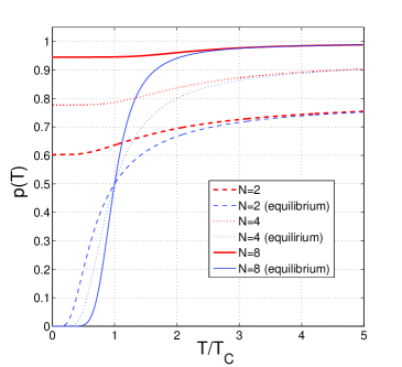
Figure 2: Population as a function of the temperature using a linear cooling for different number of particles $N=2,4$ and $8$, with $V=1.0$, $\varepsilon=1$, $R=1.4$ and $T_{0}/T_{c}=72$ , $g_{1}=2^{N}$, $g_{0}=1$ obtained by solving the master equation. The equilibrium population, obtained for $\delta\rightarrow 0$ is also shown, as indicated in the inset. Notice how the phase transition is built by a progressive sharpening of the jump in $p(T)$ as $N$ grows.

As a general trend, the cooling speed required to make a glass with fixed $p(0)$ increases with the system size. Also, it is possible to observe  a crossover which separates different behaviors of $p(0)$. For example, in Fig. (3), if $N=4,5,6$ and $7$, $p(0)$ begins to increase for a high $\delta$ after it reaches a plateau that begins around $\delta\approx 1$. The same increase is observed for $N=9$ and $10$, although shifted to the right in such a way that it does not appear in the current plot.  This crossover is due to the different growing speeds in Eq. (15). The first term of Eq. (15) goes to zero if,

$$\delta<<\Omega(E_{1})^{N}\frac{V}{E_{1}}e^{-^{E_{1}/T_{0}}}\equiv\delta_{c}(N),$$ (16a)

which defines a critical speed $$\delta_{c}(N) \delta>\delta_{c}(N) p(0) \delta<\delta_{c}(N) p(0)$$. For , is dominated by the first term in Eq. (15). The remaining term in Eq. (15) regulates the residual population for lower speeds . This term produces the plateau at a saturating value of ,

$$p(0)\approx\frac{1}{1+(N\epsilon/V)}\equiv p_{s}(0).$$ (17)

For a finite $N$, this implies that there are two kinds of glassy phases, one obtained for intermediate cooling rates in which $p(0)$ reaches a limiting value. The other kind is obtained for $\delta>\delta_{c}(N)$.

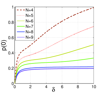
Figure 3: Residual population at $T=0$ as a function of the cooling speed for different number of particles $N=10,15,20,25$ and $30$, with $V=0.5$, $\varepsilon=1$, $R=1.4$, $g_{1}=2^{N}$, $g_{0}=1$ and $T_{0}/T_{c}=72$.

However, since $p_{s}(0)$ goes to zero as $N\rightarrow\infty$, $\delta_{c}(N)$ turns out to be the minimal speed required to make a glass in the thermodynamical limit, and leads to a critical $R_{c}$,

$$R_{c}=\Omega(E_{1})^{N}\left(\frac{T_{0}}{E_{1}}\right)e^{-^{E_{1}/T_{0}}}\Gamma_{0}.$$ (18)

From an analysis of Eq. (2) and Eq. (1), it is easy to see that $R_{c}$ is basically the inverse relaxation time for crystalization. Although it is surprising that $R_{c}$ does not depend on $V$, this is a result of the assumption that $V$ does not scale with $N$. If this is the case, the term $g_{1}x_{0}^{1+\mu}$ in Eq. (13) can determine if $g_{0}x_{0}$ plays a role in the first exponential, leading to a critical speed that depends on $V$. Notice that the result is in agreement with the remarkable observation made by Phillips concerning chemical composition and minimal cooling speed required to make glassesPhillips1 , since $R_{c}$ depends on the number of metastable states. Rigidity provides such an indirect count of metastable and stable states NaumisLandscape NaumisLandscape2 .

In conclusion, we have introduced the topology of the energy landscape in a two level model of glass. As a result, we have a solvable model that has a thermodynamic phase transition for low cooling rates and a glass transition for fast cooling.

Acknowledgments. I would like to thank Denis Boyer for useful suggestions and a critical reading of the manuscript. This work was supported by DGAPA UNAM project IN100310-3. Calculations were made at Kanbalam supercomputer at DGSCA-UNAM.

References

- (1) P.W. Anderson, Science 267, 1615 (1995).
- (2) J.C. Phillips, Rep. Prog. Phys. 59 1133 (1996).
- (3) M. Micoulaut, G.G. Naumis, Europhys Lett. 47, 568 (1999).
- (4) R. Kerner, G.G. Naumis, J. of Phys: Condens. Matter 12, 1641 (2000).
- (5) John C. Mauro, Douglas C. Allan, and Marcel Potuzak, Phys. Rev. B 80, 094204 (2009)
- (6) Morten M. Smedskjaer, John C. Mauro, and Yuanzheng Yue, Phys. Rev. Lett. 105, 115503 (2010).
- (7) Pedro E. Ramírez-González, Leticia López-Flores, Heriberto Acuña-Campa, and Magdaleno Medina-Noyola, Phys. Rev. Lett. 107, 155701 (2011)
- (8) P.G. Debenedetti, Metastable Liquids, Princeton Unv. Press, 1996.
- (9) P.G. Debenedetti and F.H. Stillinger, Nature 410, 259 (2000).
- (10) J.C. Phillips, J. Non–Cryst. Solids 34, 153 (1979).
- (11) M.F. Thorpe, J. Non-Cryst. Solids 57, 355 (1983).
- (12) Y. Wang, J. Wells, D.G. Georgiev, P. Boolchand, K. Jackson, M. Micoulaut, Phys. Rev. Lett. 87,185503 (2001).
- (13) P. Boolchand, D.G. Georgiev, M. Micoulaut, J. of Optoelectronics and Advanced Materials 4, 823 (2002).
- (14) G.G. Naumis, Phys. Rev.B 61, R9205 (2000).
- (15) A. Huerta, G.G. Naumis, Phys. Rev. Lett. 90, 145701 (2003).
- (16) A. Huerta, G.G. Naumis, D.T. Wasan, D. Henderson, A. Trokhymchuk, J. of Chem. Phys.120, 1506 (2004).
- (17) A. Huerta, G. G. Naumis, Phys. Lett. A299, 660 (2002).
- (18) A. Huerta, G.G. Naumis, Phys. Rev. B 66, 184204 (2002).
- (19) D. Selvanathan, W.J. Bresser, and P. Boolchand, Phys. Rev. B 61, 15061 (2000).
- (20) D. Novita, P. Boolchand, M. Malki, and M. Micoulaut, Phys. Rev. Lett. 98, 195501 (2007).
- (21) D.A. Huse, D.S. Fisher, Phys. Rev. Lett. 57, 2203 (1986).
- (22) Langer, Stephen A and Sethna, James P, Phys. Rev. Lett. 61, 570 (1988).
- (23) Langer, S. A., Dorsey, A. T., & Sethna, J. P., Physical Review B 40, 345-352 (1989).
- (24) Langer, Stephen A and Sethna, James P and Grannan, Eric R, 41, 2261 (1990).
- (25) Brey J.J., Prados A., Phys. Rev. B 43, 8350 (1991).
- (26) Phillips W.A., J. Low Temp. Phys. 7, 351 (1972).
- (27) Anderson P., Halperin B., Varma C., Philos. Mag. 25, 1 (1972).
- (28) D. Chandler, Introduction to Modern Statistical Mechanics, Oxford University Press (1987).
- (29) G.G. Naumis, Phys. Rev. E 71, 026114 (2005).
- (30) G.G. Naumis, J. Non-Cryst. Solids 352, 4865 (2006).