Systematic Center-to-Limb Variation in Measured Helioseismic Travel Times and Its Effect on Inferences of Solar Interior Meridional Flows

Abstract

We report on a systematic center-to-limb variation in measured helioseismic travel times, which must be taken into account for an accurate determination of solar interior meridional flows. The systematic variation, found in time-distance helioseismology analysis using SDO/HMI and SDO/AIA observations, is different in both travel-time magnitude and variation trend for different observables. It is not clear what causes this systematic effect. Subtracting the longitude-dependent east-west travel times, obtained along the equatorial area, from the latitude-dependent north-south travel times, obtained along the central meridian area, gives remarkably similar results for different observables. We suggest this as an effective procedure for removing the systematic center-to-limb variation. The subsurface meridional flows obtained from inversion of the corrected travel times are approximately 10 m s^-1 slower than those obtained without removing the systematic effect. The detected center-to-limb variation may have important implications in the derivation of meridional flows in the deep interior, and needs a better understanding.

1 Introduction

An accurate determination of the meridional flow speed in both the solar photosphere and the solar interior is crucial to the understanding of solar dynamo and predicting solar cycle variations. For example, Dikpati et al. (2006) suggested that the slow-down of the meridional circulation during the solar-cycle maximum could change the duration of the following minimum and delay the onset of the next solar cycle. Hathaway & Rightmire (2010) found that the meridional flow speed was substantially faster during the solar minimum of Cycle 23 than during the previous minimum, and suggested that this might explain the prolonged minimum of Cycle 23. Using flux-transport dynamo model simulations, Dikpati et al. (2010) suggested that the prolonged minimum of Cycle 23 might be due to that the poleward meridional flow extended all the way to the pole in Cycle 23, unlike in Cycle 22 the flow switched to equator-ward near the latitude of $60\arcdeg$. All these works demonstrate that an accurate measurement of the meridional flow speed is very important. The photospheric meridional flow speed can be determined by tracking certain photospheric features, such as magnetic structures and supergranules (e.g., Komm et al., 1993; Hathaway & Rightmire, 2010; Hathaway et al., 2010; Gizon, 2004; Švanda et al., 2006), although it is not quite clear how well the motions of these surface features represent the photospheric plasma flows. The photospheric meridional flow speed can also be inferred from Doppler-shift measurements (e.g., Hathaway et al., 1996; Ulrich, 2010), and recently Ulrich (2010) made extensive comparisons of the meridional flow speeds obtained by different methods. The meridional flows in the solar interior are primarily determined by helioseismology, i.e., by measuring frequency shifts between poleward and equator-ward traveling acoustic waves (e.g., Braun & Fan, 1998; Krieger et al., 2007; Roth & Stix, 2008), and by use of local helioseismology techniques, namely, ring-diagram analysis and time-distance helioseismology (e.g., Giles et al., 1997; Chou & Dai, 2001; Haber et al., 2002; Zhao & Kosovichev, 2004; González Hernández et al., 2008).

The subsurface meridional flow speeds obtained by the two different local helioseismology techniques are in reasonable agreement for at least the upper 20 Mm of the convection zone (e.g., Hindman et al., 2004). However, the agreement between the two analysis techniques cannot rule out that both techniques may be affected by the same or similar systematic effects. In this Letter, we report on a systematic center-to-limb variation in helioseismic travel times measured by the time-distance helioseismology technique, which was previously unnoticed but must be taken into account in the inference of the subsurface meridional flows. Other helioseismology techniques, such as the ring-diagram analysis, may also be affected by a similar systematic effect (Rick Bogart, private communication). We develop an empirical correction procedure by measuring the center-to-limb variation along the equatorial area during the periods when the solar rotation axis is perpendicular to the line-of-sight, i.e., when the solar B-angle is close to $0\arcdeg$. This correction scheme provides consistent results for the acoustic travel times in the north-south directions measured from different HMI observables and AIA chromospheric intensity variations. We introduce our data analysis procedure and present results in §2, and discuss the results and their implications in §3.

2 Data Analysis and Results

2.1 Data Analysis Tools

To facilitate analysis of the large amount of data from the Helioseismic and Magnetic Imager (HMI; Scherrer et al., 2012; Schou et al., 2012) onboard Solar Dynamics Observatory (SDO; Pesnell et al., 2012), a time-distance helioseismology data-analysis pipeline was developed and implemented at the HMI-AIA Joint Science Operation Center (Zhao et al., 2012). Every 8 hours, the pipeline provides measurements of acoustic travel times, and generates maps of subsurface flow and wave-speed perturbations by inversion of the measured travel times, covering nearly the full-disk Sun with an area of $120\arcdeg\times 120\arcdeg$.

For the pipeline processing, we select 25 overlapping areas on the solar disk and analyze the 8-hr sequences of solar oscillation data separately for each region. Acoustic travel-time maps are obtained for 11 selected wave travel distances, and are inverted to derive maps of subsurface velocity and wave-speed perturbations from the surface to about 20 Mm in depth (Zhao et al., 2012). Then the results for individual regions are merged into nearly-full-disk maps covering $120\arcdeg$ in both longitude and latitude, with a spatial sampling of $0\fdg 12$ pixel^-1 on a uniform longitude-latitude grid. The pipeline gives acoustic travel time measurements from two different fitting techniques (Couvidat et al., 2012), and inversion results based on ray-path and Born-approximation sensitivity kernels. Both measurement uncertainties for different distances and inversion error estimates for different inversion depths are given in Zhao et al. (2012). In this Letter, only the acoustic travel times obtained from Gabor-wavelet fitting (Kosovichev & Duvall, 1997) and inversion results based on the ray-path approximation kernels are presented.

Although the pipeline is designed to analyze the HMI Dopplergrams, it can nevertheless be used to analyze other HMI observables that carry solar oscillation signals, e.g., continuum intensity, line-core intensity, and line-depth. The full-disk data from the 1600 Å and 1700 Å channels of Atmospheric Imaging Assembly (AIA; Lemen et al., 2012) onboard SDO can also be used for helioseismology studies with good accuracy (Howe et al., 2011). In this study, we compare results obtained from the four HMI observables and the AIA 1600 Å data following the same analysis procedure. This comparison helps us to identify the systematic center-to-limb variation and develop a correction method.

2.2 Center-to-Limb Variation in Measured Travel Times

The north-south ($\tau_{\mathrm{ns}}$) and west-east ($\tau_{\mathrm{we}}$) acoustic travel-time differences approximately represent the north-south and west-east flow components, respectively, although a full inversion is required to determine more precisely these flows. We first show the measured travel time differences and then present the inversion results. We choose a 10-day period of December 1 through December 10, 2010, when the solar B-angle between the equator and the ecliptic is close to $0\arcdeg$ to avoid complications caused by leakage of the solar rotation signal into the meridional flow measurements.

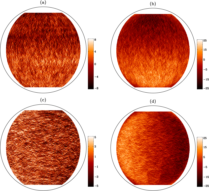
Figure 1: Travel-time maps (in unit of sec), covering $120\arcdeg$ in both longitude and latitude, for $\tau_{\mathrm{ns}}$ obtained from (a) HMI Dopplergrams and from (b) HMI continuum intensity, and for $\tau_{\mathrm{we}}$ obtained from (c) Dopplergrams and from (d) continuum intensity after a longitudinally averaged profile, representing the differential rotation, is removed through all longitudes. Note that color scales are not the same in all panels.

The upper panels of Figure 1 show the nearly-full-disk map of $\tau_{\mathrm{ns}}$, averaged over the 10-day period, measured from the HMI Dopplergram and continuum intensity data for an acoustic travel distance of $1\fdg 08-1\fdg 38$. The general pattern of positive $\tau_{\mathrm{ns}}$ in the southern hemisphere and negative $\tau_{\mathrm{ns}}$ in the northern hemisphere is usually thought to be caused by the interior poleward meridional flows. However, the apparent differences between the magnitude of $\tau_{\mathrm{ns}}$ obtained from the Doppler data and that obtained from the continuum intensity data indicate that there are additional systematic variations. The lower panels show the averaged $\tau_{\mathrm{we}}$ maps measured from the same observables after the latitude-dependent travel times caused by the differential rotation, obtained by averaging the measurements of all longitudes, are subtracted. One would expect $\tau_{\mathrm{we}}$ be relatively flat along same latitudes because the solar rotation does not vary significantly with longitude, but both $\tau_{\mathrm{we}}$ maps show systematic travel-time variations along the same latitudes, positive in the eastern hemisphere and negative in the western hemisphere. The longitudinal variation is quite significant for the measurements from the intensity data (Figure 1d) and small but not negligible for the measurements from the Dopplergram data (Figure 1c).

To more quantitatively illustrate this systematic variation, we average $\tau_{\mathrm{ns}}$ in a $20\arcdeg$-wide band along the central meridian as a function of latitude, and display the averaged curves in the top panels of Figure 2 for three selected measurement distances and for the four HMI observables: Doppler velocity, continuum intensity, line-core intensity, and line-depth. In the middle-row panels, we show the corresponding $\tau_{\mathrm{we}}$ curves obtained by averaging over a $20\arcdeg$-wide band along the equator as a function of longitude (hereafter, longitude is relative to the central meridian). If there were no systematic center-to-limb variation in the measured acoustic travel times, $\tau_{\mathrm{ns}}$ obtained from the different observables would agree with each other, and $\tau_{\mathrm{we}}$ would remain flat for all observables. But clearly, the measurements are not as expected. Among all these measurements, the $\tau_{\mathrm{ns}}$ curves show not only different magnitude of travel-time shifts but sometimes also opposite variation trends. For $\tau_{\mathrm{we}}$, it is found that the measurements from the Dopplergrams have the smallest systematic variations and are similar to the line-core intensity measurements at larger distances. However, the travel times measured from the continuum intensity and line-depth data show not just substantial travel-time shifts for all measurement distances but also opposite center-to-limb variations. It is quite clear that the travel-time variations along the equator are not caused by solar flow but represent a systematic center-to-limb variation. If we treat the longitude-dependent $\tau_{\mathrm{we}}$ variations along the equatorial area as the systematic center-to-limb variations, and subtract these variations from the latitude-dependent $\tau_{\mathrm{ns}}$ measured using the corresponding observables, we get the residual curves shown in the bottom-row panels of Figure 2. It is remarkable that for all the measurement distances, the results from all four HMI observables are in reasonable agreement. This suggests that the residual travel times correspond to the subsurface meridional flow signals.

It was demonstrated that the SDO/AIA 1600 Å data are also suitable to perform helioseismology analysis (Howe et al., 2011). Figure 3 shows a comparison of the results obtained from the HMI Dopplergrams and the AIA 1600 Å data for one selected measurement distance, $3\fdg 12-3\fdg 84$. Similarly, $\tau_{\mathrm{ns}}$ measured from the AIA 1600 Å data also differ from that measured from the HMI Dopplergram. The $\tau_{\mathrm{we}}$ measured from the AIA data also show systematic variations, though its longitudinal trend is opposite to that measured from HMI continuum intensity and the variation magnitude is much smaller. The residual, obtained after subtracting the longitude-dependent $\tau_{\mathrm{we}}$ from the latitude-dependent $\tau_{\mathrm{ns}}$ for AIA 1600 Å, is quite similar to that obtained from the HMI Dopplergrams and other HMI observables. This result is particularly remarkable because HMI and AIA are different instruments observing in different spectral lines: AIA in 1600 Å and HMI in Fe I 6173 Å, which are formed at different heights in the solar atmosphere.

2.3 Effect on Meridional Flow Inversions

The systematic center-to-limb travel-time variations would have an apparent effect on the inference of subsurface meridional flows obtained by inversion. Here, we investigate how the inferred meridional flow speed changes after removal of this systematic effect.

We employ the time-distance helioseismology pipeline code developed for inversion of the acoustic travel times (Zhao et al., 2012). The inversion results are shown in Figure 4. The middle row of Figure 4 presents inversion results obtained from travel-time measurements shown in Figure 2, but with an extension of $15\arcdeg$ closer to both poles and both limbs to better illustrate that the removal of the systematic effect also helps to improve inversions in high-latitude areas. The top and bottom rows of Figure 4 show results obtained from June 1 – 10, 2010 and June 1 – 10, 2011, when the solar B-angle were also close to 0$\arcdeg$. It can be seen from left columns of Figure 4 that above $\sim 55\arcdeg$ latitude, the inferred meridional flow drops in speed and becomes equator-ward for the depth of 0 – 1 Mm, but remains pole-ward deeper than 3 Mm. This is a suspicious behavior for the meridional flows. We then antisymmetrize the east-west direction velocity caused by the center-to-limb variations (middle column of Figure 4), and subtract it from the inferred meridional velocity. The residual subsurface meridional flows show much more consistent behaviors at different depths in high-latitude areas (right column of Figure 4). From Figure 4, one can also find that the center-to-limb variation measured from equatorial area also slightly change with time, and why there is such a change is not understood and worth further studies.

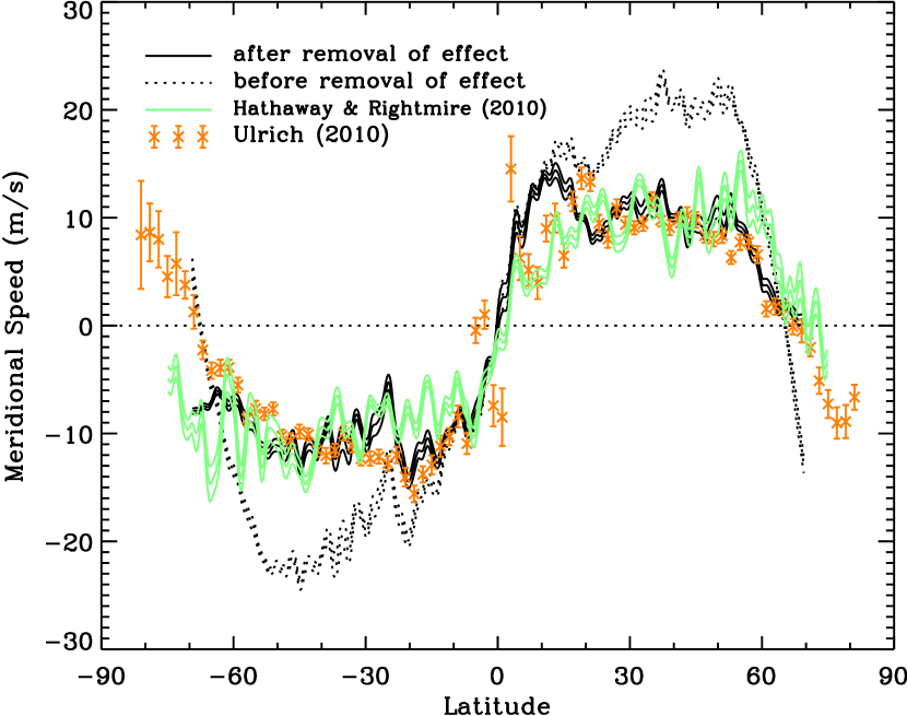
Figure 5: Comparison of the meridional flow speed obtained by magnetic feature tracking (Hathaway & Rightmire, 2010), from surface Doppler measurements (Ulrich, 2010), and obtained in this study for a depth of 0 – 1 Mm before and after the removal of the systematic effect. Our results are from a 10-day period, December 1 – 10, 2010, and are displayed after spatial averaging. The results from magnetic feature tracking and from Doppler measurement are averaged over a 6-month period with our analyzed period in the middle.

The removal of the center-to-limb variation in the measured travel times also decreases the inferred flow speed by nearly 10 m s^-1. This indicates that the subsurface meridional flows derived from the previous time-distance studies (e.g., Zhao & Kosovichev, 2004) might have overestimated the flow speed by a large fraction. Figure 5 shows that after removal of the systematic effect, the meridional flow speed is closer in magnitude to the results obtained by the magnetic feature tracking (Hathaway & Rightmire, 2010) and surface Doppler measurements (Ulrich, 2010). Note that the results from the magnetic feature tracking and from the MWO Doppler observations shown in Figure 5 are both averaged over a 6-month period with our analyzed 10-day period in the middle. The difference of analysis period may result in some differences seen in the figure. The meridional flows obtained from this study are displayed in Figure 5 after a $2\arcdeg$ spatial averaging to remove the strong fluctuations caused by supergranular flows.

3 Discussion

The analysis of acoustic travel times obtained from different observables of the HMI and AIA instruments on SDO by the time-distance helioseismology technique has revealed a systematic center-to-limb variation. The systematic variation is different for different observables, and range from $\sim$2 sec for the HMI Dopplergram to $\sim$10 sec for the continuum intensity measurements. For an accurate determination of subsurface meridional flows, and also for more accurate inference of full-disk subsurface flow fields, this systematic effect should be removed. We have developed an empirical correction procedure by removing the systematic variation measured along the equatorial area during the period when solar B-angle is close to $0\arcdeg$. This correction reconciles the latitude-dependent $\tau_{\mathrm{ns}}$ measured from different observables and reduces the inferred meridional flow speed by about 10 m s^-1.

It is not quite clear what causes this systematic center-to-limb effect. However, this effect is unlikely caused by instrumental or data calibration, because it is observed in the data from two different instruments, HMI and AIA, and it exists in different observables of HMI. We also rule out the following factors as causes of this effect: finite speed of light, contribution of horizontal wave component, and foreshortening effect. Due to the finite speed of light, acoustic wave signals observed at high latitude and observed near the equator are not simultaneous, but this effect is negligible given the small measurement distances used in this study. The horizontal wave component (Nigam et al., 2007) is used to explain the center-to-limb variation in mean travel times observed by Duvall (2003), but this effect is not significant in travel-time differences for waves traveling in opposite directions and in small distances as used in this study. To check foreshortening effects, we mimicked the high-latitude data by reducing the spatial resolution of the data observed at lower latitudes, and our measurements did not show systematic changes in the measured travel times similar to the center-to-limb variations reported here.

It is more likely that this effect has a physical origin related to properties of solar acoustic waves in the solar atmosphere or response of the spectral lines to the solar oscillations. It is well known that for a given spectral line the Sun is observed at the same optical depth but not at the same geometrical height. The observed height gradually increases with distance from the disk center. Thus it is possible that the acoustic waves traveling in opposite directions and different height will give different measured travel times due to the subsurface location of the wave source and the waves evanescent behavior above the photosphere (Nagashima et al., 2009). However, this cannot explain why different observables give different magnitude and trend of the center-to-limb variations. Another interesting fact is that the largest systematic effect exists in the measurements using HMI continuum that forms at the lowest height in the atmosphere. As one moves up to the height where Doppler velocity is measured, the systematic effect is reduced. As the measurements move further up to where AIA 1600 Å is formed, the effect reverses sign. This may give us some indication of that this center-to-limb variation is related to the line formation height. It is also possible that this systematic effect is related to differences in the acoustic power distributions, line-asymmetry of solar modes (Duvall et al., 1993), and the correlated noise effect (Nigam et al., 1998). The cause of this systematic effect is worth further studies, and may be resolved by numerical modeling of solar oscillations including the spectral line-formation simulation and spherical geometry of the Sun. It is worth attention that when inferring meridional flow velocity from surface Doppler measurements, a systematic center-to-limb velocity profile also needs to be removed (Ulrich et al., 1988; Ulrich, 2010). A similar limb-shift effect very likely exists in the HMI Dopplergrams that are used in our time-distance measurements, and it is not clear whether this effect accounts for some of the systematic variations in our measured acoustic travel times. This is worth further studies.

Although the cause of this systematic center-to-limb variation is not well understood, it is demonstrated that the empirical correction procedure can improve the inferred subsurface meridional flows. Figures 2 – 4 demonstrate that subtracting the longitude-dependent $\tau_{\mathrm{we}}$ from the latitude-dependent $\tau_{\mathrm{ns}}$, measured from same observables, is an effective way to remove this systematic effect. This correction procedure helps to reconcile the $\tau_{\mathrm{ns}}$ measured from different observables, and also helps to remove the inconsistent behaviors of meridional flows in high-latitude areas. As an effect, the newly obtained subsurface meridional flows at shallow depths are approximately 10 m s^-1 slower than the speed previously derived following a similar analysis procedure. This systematic center-to-limb variation in measured acoustic travel times has an important implication in the long-searched deep equator-ward meridional flows, and this is currently under investigation.

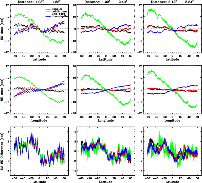
Figure 2: Top: Averaged curves of latitude-dependent $\tau_{\mathrm{ns}}$, obtained from different HMI observables and for different measurement distances. Middle: Averaged curves of longitude-dependent $\tau_{\mathrm{we}}$, obtained from different observables and for different measurement distances. Bottom: Differences of $\tau_{\mathrm{ns}}$ and $\tau_{\mathrm{we}}$. Note that the vertical scales for the upper two rows are different from those for the bottom row.

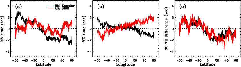
Figure 3: (a) Averaged latitude-dependent $\tau_{\mathrm{ns}}$, obtained from HMI Dopplergrams and from AIA 1600 Å data for a measurement distance of $3\fdg 12-3\fdg 84$. (b) Averaged longitude-dependent $\tau_{\mathrm{we}}$ for these two observables. (c) Differences of $\tau_{\mathrm{ns}}$ and $\tau_{\mathrm{we}}$.

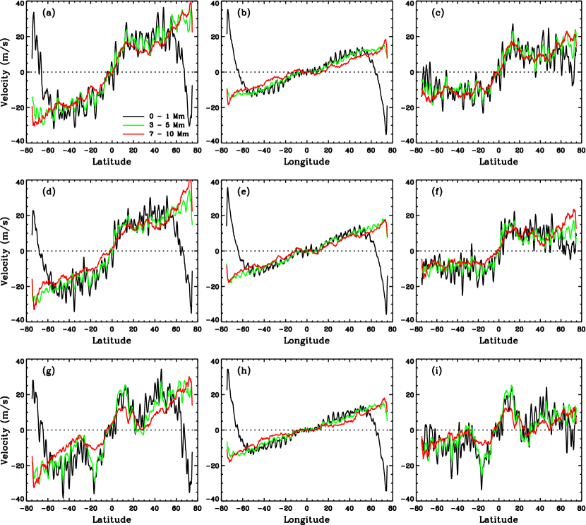
Figure 4: Results obtained from the periods of June 1 – 10, 2010 (top row), December 1 – 10, 2010 (middle row), and June 1 – 10, 2011 (bottom row). (a) Meridional flow velocity for different depths, obtained by inversions of acoustic travel times measured from the HMI Dopplergram and without removal of the systematic center-to-limb variations. (b) Antisymmetrized east-west velocity obtained by inversion, representing the center-to-limb variations. (c) Meridional flow velocities after removal of the systematic center-to-limb variations. (d) – (f) and (g) – (i) are the same as (a) – (c) but for different time periods.

References

- Braun & Fan (1998) Braun, D. C., & Fan, Y. 1998, ApJ, 508, L105
- Chou & Dai (2001) Chou, D.-Y., & Dai, D.-C. 2001 ApJ, 559, L175
- Couvidat et al. (2012) Couvidat, S., Zhao, J., Birch, A. C., Kosovichev, A. G., Duvall, T. L., Jr., Parchevsky, K., & Scherrer, P. H. 2012, Sol. Phys., 275, 357
- Dikpati et al. (2006) Dikpati, M., de Toma, G., & Gilman, P. A. 2006, Geophys. Res. Lett., 330, L05102
- Dikpati et al. (2010) Dikpati, M., Gilman, P. A., de Toma, G., & Ulrich, R. K. 2010, Geophys. Res. Lett., 37, L14107
- Duvall (2003) Duvall, T. L., Jr. 2003, in: Proc. of SOHO 12/ GONG+ 2002, ed. H. Sawaya-Lacoste, ESA SP-517, Noordwijk, Netherlands, 259
- Duvall et al. (1993) Duvall, T. L., Jr., Jefferies, S. M., Harvey, J. W., Osaki, Y., & Pomerantz, M. A. 1993, ApJ, 410, 829
- Giles et al. (1997) Giles, P. M., Duvall, T. L., Jr., Scherrer, P. H., & Bogart, R. S. 1997, Nature, 390, 52
- Gizon (2004) Gizon, L. 2004, Sol. Phys., 224, 217
- González Hernández et al. (2008) González Hernández, I., Kholikov, S., Hill, F., Howe, R., & Komm, R. 2008, Sol. Phys., 252, 235
- Haber et al. (2002) Haber, D. A., Hindman, B. W., Toomre, J., Bogart, R. S., Larsen, R. M., & Hill, F. 2002, ApJ, 570, 855
- Hathaway & Rightmire (2010) Hathaway, D. H., & Rightmire, L. 2010, Science, 327, 1350
- Hathaway et al. (2010) Hathaway, D. H., Williams, P. E., Dela Rosa, K., & Cuntz, M. 2010, ApJ, 725, 1082
- Hathaway et al. (1996) Hathaway, D. H., et al. 1996, Science, 272, 1306
- Hindman et al. (2004) Hindman, B. W., Gizon, L., Duvall, T. L., Jr., Haber, D. A., & Toomre, J. 2004, ApJ, 613, 1253
- Howe et al. (2011) Howe, R., Hill, F., Komm, R., Broomhall, A.-M., Chaplin, W. J., & Elsworth, Y. 2011, J. of Phys. Conf. Ser., 271, 012058
- Krieger et al. (2007) Krieger, L., Roth, M., & von der Lühe, O. 2007, Astronomische Nachrichten, 328, 252
- Komm et al. (1993) Komm, R. W., Howard, R. F., & Harvey, J. W. 1993, Sol. Phys., 147, 207
- Kosovichev & Duvall (1997) Kosovichev, A. G., & Duvall, T. L., Jr. 1997, in Proceedings of SCORe’96 Workshop: Solar Convection and Oscillations and Their Relationship, ed. F. P. Pijpers, J. Christensen-Dalsgaard & C. S. Rosenthal (Dordrecht: Kluwer), 241
- Lemen et al. (2012) Lemen, J. R., Title, A. M., Akin, D. J., Boerner, P. F., Chou, C., Drake, J. F., Duncan, D. W., Edwards, C. G., Friedlaender, F. M., Heyman, G. F., et al. 2012, Sol. Phys., 275, 17. DOI: 10.1007/s11207-011-9776-8
- Nagashima et al. (2009) Nagashima, K., Sekii, T., Kosovichev, A. G., Zhao, J., & Tarbell, T. D. 2009, ApJ, 694, L115
- Nigam et al. (2007) Nigam, R., Kosovichev, A. G., & Scherrer, P. H. 2007, ApJ, 659, 1736
- Nigam et al. (1998) Nigam, R., Kosovichev, A. G., Scherrer, P. H., & Schou, J. 1998, ApJ, 495, L115
- Pesnell et al. (2012) Pesnell, W. D., Thompson, B. J., & Chamberlin, P. C. 2012, Sol. Phys., 275, 3. DOI: 10.1007/s11207-011-9841-3
- Roth & Stix (2008) Roth, M., & Stix, M. 2008, Sol. Phys., 251, 77
- Scherrer et al. (2012) Scherrer, P. H., Schou, J., Bush, R. I., Kosovichev, A. G., Bogart, R. S., Hoeksema, J. T., Liu, Y., Duvall, T. L., Jr., Zhao, J., Title, A. M., et al. 2012, Sol. Phys., 275, 207. DOI: 10.1007/s11207-011-9834-2
- Schou et al. (2012) Schou, J., Scherrer, P. H., Bush, R. I., Wachter, R., Couvidat, S., Rabello-Soares, M. C., Bogart, R. S., Hoeksema, J. T., Liu, Y., Duvall, T. L., Jr., et al. 2012, Sol. Phys., 275, 229. DOI: 10.1007/s11207-011-9842-2
- Švanda et al. (2006) Švanda, M., Klvaňa, M., & Sobotka, M. 2006, A&A, 458, 301
- Ulrich (2010) Ulrich, R. K. 2010, ApJ, 725, 658
- Ulrich et al. (1988) Ulrich, R. K., Boyden, J. E., Webster, L., Padilla, S. P., & Snodgrass, H. B. 1988, Sol. Phys., 117, 291
- Zhao et al. (2012) Zhao, J., Couvidat, S., Bogart, R. S., Parchevsky, K. V., Birch, A. C., Duvall, T. L., Jr., Beck, J. G., Kosovichev, A. G., Scherrer, P. H. 2012, Sol. Phys., 275, 375. DOI: 10.1007/s11207-011-9757-y
- Zhao & Kosovichev (2004) Zhao, J., & Kosovichev, A. G. 2004, ApJ, 603, 776