Local Heuristic for the Refinement of Multi-Path Routing in Wireless Mesh Networks

Abstract

We consider wireless mesh networks and the problem of routing end-to-end traffic over multiple paths for the same origin-destination pair with minimal interference. We introduce a heuristic for path determination with two distinguishing characteristics. First, it works by refining an extant set of paths, determined previously by a single- or multi-path routing algorithm. Second, it is totally local, in the sense that it can be run by each of the origins on information that is available no farther than the node’s immediate neighborhood. We have conducted extensive computational experiments with the new heuristic, using AODV and OLSR, as well as their multi-path variants, as underlying routing methods. For two different CSMA settings (as implemented by 802.11) and one TDMA setting running a path-oriented link scheduling algorithm, we have demonstrated that the new heuristic is capable of improving the average throughput network-wide. When working from the paths generated by the multi-path routing algorithms, the heuristic is also capable to provide a more evenly distributed traffic pattern.

Keywords: Wireless mesh networks, Multi-path routing, Path coupling, Disjoint paths, Mutual interference.

1 Introduction

Wireless mesh networks (WMNs) have lately been recognized as having great potential to provide the necessary networking infrastructure for communities and companies, as well as to help address the problem of providing last-mile connections to the Internet [33, 43]. However, mutual radio interference among the network’s nodes can easily reduce the throughput as network density grows above a certain threshold [7] and therefore compromise the entire endeavor. Such interference is caused by the attempted concomitant communication among nodes of the same network and constitutes the most common cause of the network’s throughput’s falling short of being satisfactory (hardly reaching a fraction of that of a wired network [21]). A promising approach to tackle the reduction of mutual interference seems to be to combine routing algorithms with some interference avoidance approach, such as power control, link scheduling, or the use of multi-channel radios [2]. In fact, this type of network interference problem has been addressed by a considerable number of different strategies to be found in the literature [12, 13, 1, 41, 11, 51, 44, 4].

An alternative approach that presents itself naturally is the use of multi-path routing to distribute traffic among multiple paths sharing the same origin and the same destination, since in principle it can help with both path recovery and load balancing better than the use of single-path strategies. It may, in addition, lead to better throughput values over the entire network [26, 5]. But while these benefits accrue only insofar as they relate to how the multiple paths interfere with one another [46, 45], unfortunately this aspect of the problem is not commonly addressed by multi-path strategies. What happens as a consequence is that, though promising by virtue of adopting multiple paths to accommodate the same end-to-end traffic, in general such strategies fail to perform as desired because they do not tackle the interference problem during path discovery. The single noteworthy exception here seems to be the algorithm reported in [49], but it uses geographic information (like localization aided by GPS) to find paths with sufficient spatial separation so as not to interfere with one another. In our view this weakens the approach somewhat, since such type of information may not always be available [14]. Moreover, the corresponding algorithm relies on the solution of an NP-hard problem on an input that has the size of the network [50], so the solution may be unattainable in practice.

Here we propose a different approach to alleviate the effects of interference in multi-path routing. Our approach is based on two general principles. First, that it is to work as a refinement phase over existing routing algorithms, thereby inherently preserving, to the fullest possible extent, the advantages of any given routing method. Second, that it is to rely only on information that is locally available to the common origin of any given set of multiple paths leading to the same destination. That is, only information that the origin can obtain by communicating with its direct neighbors in the WMN should be used. One intended consequence of the latter, in particular, is that refining the set of paths departing from any common origin should be easily implementable by straightforward message passing, and moreover, that any required calculation by that node should be amenable to being carried out efficiently even if it involves the solution of a computationally difficult problem. In order to comply with these two principles, our approach operates on a previously established set of paths leading from a common origin, say $i$, to a common destination, say $j$. It operates exclusively on the neighborhood information stored at node $i$ itself or at any of its neighbors, say $k$, such that $k$ participates in some of the $i$-to-$j$ paths, as well as on the information stored at these same nodes regarding the routing of packets to node $j$. Once node $i$ has acquired all this information, an undirected graph $G_{ij}$ is constructed that represents every possible interference that can occur as packets get forwarded toward $j$ by those of $i$’s neighbors that are on $i$-to-$j$ paths. Solving a well-known NP-hard problem (that of finding a maximum weighted independent set) on this typically small graph serves as a heuristic to decide which of the $i$-to-$j$ paths to keep and which to discard.

It is important to note that, being determined with reference to graph $G_{ij}$, the resulting set contains no two paths that interfere with each other as far as node $i$’s neighbors are concerned, except of course for the inevitable interference that may occur as packets leave $i$ or reach $j$. In our view, this provides a sharp contrast between our approach and others that aim at weaker forms of independence between the paths, for example by seeking paths that are merely edge- or node-disjoint [27, 28, 47, 13, 3, 41, 52, 30, 51, 53]. This is so because, as remarked elsewhere (e.g., [37]), independence by edge-disjointness encompasses independence by node-disjointness, which in turn encompasses independence by noninterference. Of course, the highest an independence relation’s level in this hierarchy the easiest it is to implement it as the multiple paths are discovered (not coincidentally, the simple exchange of tokens between nodes suffices to produce edge- or node-disjoint path sets [29]).

We proceed in the following manner. First we state the problem in graph-theoretic terms and give our solution in Section 2. Then we move, in Section 3, to a presentation of the methodology we followed in conducting our computational experiments. Our results are given in Section 4 and involve comparisons with some prominent routing algorithms, viz. AODV [38], AOMDV [31], OLSR [23], and MP-OLSR [54]. We used these algorithms both as stand-alone methods and as bases to our own heuristic. Our results include throughput and fairness [24] comparisons based both on NS2.34 [35] simulations and on the SERA link scheduling algorithm [48]. We continue in Section 5 with further discussions and conclude in Section 6.

2 Problem formulation and heuristic

For $i$ and $j$ any two distinct nodes of the WMN, we begin by assuming that some routing protocol already established a set $\mathcal{P}_{ij}$ of paths directed from $i$ to $j$. Another key element is that, since we seek to establish independence by noninterference, an interference model, along with its assumptions, must be selected. Our choice is the protocol-based interference model, together with the assumption that a node’s communication and interference radii are the same. Should a different model be selected or the two radii be significantly different, the only effect would be for the graph construction process outlined below, once adapted accordingly, to produce a different graph (in particular, the interference radius could be chosen appropriately in order for the protocol-based interference model to mimic the physical interference model [42]).

Under the assumptions of the protocol-based interference model, the communication/interference radius is fixed at some value $R$, which we take to be the same for all nodes. It follows that two nodes are neighbors of each other in the WMN if and only if the Euclidean distance between them is no greater than $R$. Moreover, since every link may transmit in both directions for error control, it also follows that two links can interfere with each other if either one’s transmitter or receiver is a neighbor of the other’s transmitter or receiver [8]. As will become apparent shortly, this has important implications when modeling interference, since links that share no nodes can still interfere with one another.

In keeping with the locality principle outlined in Section 1, we work on the premise that a node $k$’s knowledge is limited to the set $N_{k}$ of its neighbors and the set $\mathrm{Next}_{k}(i,j)\subseteq N_{k}$ of neighbors to which it may forward packets sent by node $i$ to node $j$ (assuming $k\neq j$). Set $\mathrm{Next}_{k}(i,j)$, obviously, depends on the $j$-bound paths that leave $i$ and go through node $k$. The problem we study is that of eliminating from $\mathcal{P}_{ij}$ the fewest possible paths (in a weighted sense, to be discussed later) so that the remaining path set, henceforth denoted by $\mathcal{P}^{\mathrm{R}}_{ij}$, contains no mutually interfering paths except at $i$ or $j$. However, owing once again to the issue of locality, we forgo both optimality and feasibility a priori and settle for a heuristic instead. That is, for the sake of locality we admit the possibility that, in the end, neither will the selected paths be collectively optimal nor will the absence of interference among them be guaranteed (except at those paths’ second hops, which will be non-interfering relative to one another necessarily).

Before proceeding, we tackle two special cases. The first one is that in which $\mathcal{P}_{ij}$ contains the single-link path that connects $i$ directly to $j$. In this case, we let $\mathcal{P}^{\mathrm{R}}_{ij}$ be the singleton that contains that path, since no other arrangement can possibly do better. The second special case is that in which $|\mathcal{P}_{ij}|=1$, provided the single path contained in $\mathcal{P}_{ij}$ has at least two links, and is motivated by the situations in which $\mathcal{P}_{ij}$ originates from single-path routing. In this case, we enlarge $\mathcal{P}_{ij}$ before feeding it to our path-selection heuristic. Letting node $k$ be such that $\mathrm{Next}_{i}(i,j)=\{k\}$, we do this enlargement of $\mathcal{P}_{ij}$ by including in it as many paths from $\mathcal{P}_{kj}$ as possible, each suitably prefixed by the new origin $i$, provided none of the new paths is weightier than the one initially in $\mathcal{P}_{ij}$. If enlargement turns out to be impossible, then the problem becomes moot for $\mathcal{P}_{ij}$ and we let $\mathcal{P}^{\mathrm{R}}_{ij}=\mathcal{P}_{ij}$.

We are then in position to introduce our refinement algorithm for multi-path routing, henceforth referred to by the acronym MRA (for multi-path refinement algorithm). The goal of MRA is to create an undirected graph $G_{ij}$ corresponding to the path set $\mathcal{P}_{ij}$ and to extract from it the information necessary to determine $\mathcal{P}^{\mathrm{R}}_{ij}$. This graph’s node set, henceforth denoted by $V$, has one node for each of the paths in $\mathcal{P}_{ij}$. Its edge set, denoted by $E$, is constructed in such a way as to represent every interference possibility that can be inferred solely from the sets $N_{k}$ and $\mathrm{Next}_{k}(i,j)$ for every $k\in N_{i}$ that participates in at least one of the paths in $\mathcal{P}_{ij}$. Once graph $G_{ij}$ is built, finding a maximum weighted independent set in it (i.e., a subset of $V$ containing no two nodes joined by an edge in $E$ and being as weighty as possible) provides the best possible approximate decision on which of the paths in $\mathcal{P}_{ij}$ should constitute $\mathcal{P}^{\mathrm{R}}_{ij}$, namely those corresponding to the nodes in the maximum weighted independent set that was found.

MRA proceeds as given next, following the introduction of some auxiliary nomenclature. Given two neighboring WMN nodes, say $k$ and $k^{\prime}$, we are interested in the following two possibilities for the pair $k,k^{\prime}$. A type-A pair is part of at least one path in $\mathcal{P}_{ij}$ in such a way that $k^{\prime}\in\mathrm{Next}_{k}(i,j)$ with $k\in N_{i}$ or $k\in\mathrm{Next}_{k^{\prime}}(i,j)$ with $k^{\prime}\in N_{i}$. In a type-B pair, both $k$ and $k^{\prime}$ belong to at least one path in $\mathcal{P}_{ij}$ as well, but not the same path. Moreover, at least one of them is a member of $N_{i}$ while the other, if not in $N_{i}$ as well, is in $\mathrm{Next}_{l}(i,j)$ for some other $l\in N_{i}$. Note that type-A and -B pairs constitute all the structural information that node $i$ can gather by strictly local communication from its neighborhood $N_{i}$ in the WMN. In the case of a type-A pair, we let $\mathrm{Paths}(k,k^{\prime})$ be the set of $i$-to-$j$ paths to which the pair belongs.

1. Let $V$ have one node for each path in $\mathcal{P}_{ij}$. Add one further node to $V$ for each type-B pair of neighboring WMN nodes. We refer to these additional nodes as temporary nodes.

2. Construct $E$ as follows:

   1. Let $k,k^{\prime}$ and $l,l^{\prime}$ be two pairs of neighboring WMN nodes, each pair being of type A or B. If it holds that $k=l$, $k=l^{\prime}$, $k^{\prime}=l$, or $k^{\prime}=l^{\prime}$, then add an edge to $E$ between each node corresponding to a path in $\mathrm{Paths}(k,k^{\prime})$ (if the pair is of type A) or the corresponding temporary node (if the pair is of type B) to each node corresponding to a path in $\mathrm{Paths}(l,l^{\prime})$ (if the pair is of type A) or the corresponding temporary node (if the pair is of type B).

   2. Connect any two nodes in $V$ by an edge if, after the previous step, the distance between them is $2$.

   3. Remove all temporary nodes from $V$ and all edges that touch them from $E$.

3. Find a maximum weighted independent set of $G_{ij}$ and output $\mathcal{P}^{\mathrm{R}}_{ij}$ accordingly.

In these steps, graph $G_{ij}$ starts out as a graph with $|\mathcal{P}_{ij}|$ nodes and gets enlarged by the addition of temporary nodes that represent some of the possibilities of off-path interference as nodes in $N_{i}$ engage in transmitting packets (Step (1)). Then it receives edges to account for the assumptions of the protocol-based interference model (Steps (2).i and (2).ii) and is after that stripped of all temporary nodes to end up with $|\mathcal{P}_{ij}|$ nodes once again (Step (2).iii). Step (2).ii, in particular, accounts for interference in the WMN when a link’s transmitter or receiver does not coincide with (but is a neighbor of) another link’s transmitter or receiver. The last MRA step, Step (3), is the determination of a maximum weighted independent set of $G_{ij}$. We use node weights such that, for the node corresponding to path $p\in\mathcal{P}_{ij}$, the weight is $1/C_{p}$, where $C_{p}$ is the path’s hop count. In other words, shorter paths tend to be favored over longer ones as $\mathcal{P}^{\mathrm{R}}_{ij}$ is extracted from $\mathcal{P}_{ij}$. Clearly, though, any other desired criterion can be used as well. An illustration of how MRA works is given in Fig. 1.

Figure 1: Construction of graph $G_{ij}$ for the path set $\mathcal{P}_{ij}=\{a,b,c,d,e\}$. The paths in $\mathcal{P}_{ij}$ are shown in panel (a), where each directed edge leads to a node in some $\mathrm{Next}(i,j)$ set (for example, $\mathrm{Next}_{k_{1}}(i,j)=\{j,k_{5}\}$) and each dashed edge joins neighboring nodes that share none of the $i$-to-$j$ paths. We see in this panel that $\mathrm{Paths}(k_{2},k_{6})=\{b,c\}$, and also that there are five type-A node pairs ($k_{1},j$; $k_{2},k_{6}$; $k_{2},k_{3}$; $k_{1},k_{5}$; and $k_{4},k_{6}$) as well as one single type-B node pair ($k_{3},k_{5}$, labeled $x$). Panel (b) shows graph $G_{ij}$ as it stands after Steps (1) and (2).i, respectively for creating its node set $V$ and initializing its edge set $E$ as a function of node coincidence among all type-A or -B pairs. The distance-$2$ closure determined in Step (2).ii is shown in panel (c), with the additional edges represented as dashed lines. Panel (d), finally, shows $G_{ij}$ as it stands at the end, after Step (2).iii. Notice, in particular, the fundamental role played by node $x$ in identifying the interference between paths $c$ and $d$ under the protocol-based interference model (it is through $x$, as the distance-$2$ closure is determined, that $c$ and $d$ become connected). If equal weights were used for all nodes, then clearly any of $\{a,b\}$, $\{a,c\}$, $\{a,e\}$, $\{b,d\}$, or $\{d,e\}$ would qualify as a maximum weighted independent set of $G_{ij}$ in Step (3). However, using $1/C_{p}$ as the weight of the node corresponding to path $p$ leads to $\{a,b\}$ and $\{a,e\}$ as the only possibilities, each of total weight $1/2+1/3=5/6$, since $C_{a}=2$ and $C_{b}=C_{e}=3$. In the end, then, we have either $\mathcal{P}^{\mathrm{R}}_{ij}=\{a,b\}$ or $\mathcal{P}^{\mathrm{R}}_{ij}=\{a,e\}$, each set containing paths whose second hops do not interfere with one another, each set as large as possible in the weighted sense provided by the use of $1/C_{p}$.

3 Methods

We evaluated the performance of MRA through extensive experimentation with the following routing algorithms: AODV [38], AOMDV [31], OLSR [23], and MP-OLSR [54]. For the purpose of conciseness, we henceforth refer to the combination of each of these algorithms with MRA as R-AODV, R-AOMDV, R-OLSR, and R-MP-OLSR, respectively. We remark that, since both AODV and OLSR are single-path routing algorithms, handling the paths they generate falls into one of the special cases discussed in Section 2. Our experiments were run in the network simulator NS2.34 (NS2 henceforth) [35] and in a simulator that employs the SERA link scheduling algorithm [48], briefly described later in this section. We used two different configurations of routing-algorithm parameters, and likewise two different configurations of NS2 parameters (one for the path-discovery process and another for performance evaluation). These configurations were selected during initial tuning experiments and will be presented shortly.

3.1 Topology generation

We generated four types of network according to the maximum number of neighbors, $\Delta$, a node may have. Each network was generated by placing $n$ nodes inside a square of side $1500$. The first of these nodes was positioned at the center of the square and the remaining nodes were placed randomly as a function of the communication/interference radius $R$ introduced at the beginning of Section 2. Their placement was subject to the constraints that each node would have at least one neighbor, that no node would be closer to any other than $25$ units of Euclidean distance, and that no node would have more than $\Delta$ neighbors. No more than $1000$ attempts at positioning nodes were allowed; if this limit was reached then the growing network was discarded and the generation of a new one was started. The value of $R$ was determined so that the expected density of nodes inside a radius-$R$ circle would be proportional to $\Delta/R^{2}$ (assuming some uniformly random form of placement), and be moreover about the same density as that of the whole network. It follows that $\Delta/R^{2}\propto n$. We chose the proportionality constant to yield $R=200$ for $n=80$ and $\Delta=4$, whence $R=200\sqrt{20\Delta/n}$. Of all the networks generated, there are $100$ networks for each combination of $n\in\{60,80,100,120\}$ and $\Delta\in\{4,8,16,32\}$, thus totaling $1600$ networks.

3.2 Path discovery

For each of the $1600$ networks we randomly generated $100$ sets of node pairs to function as origin-destination pairs (instances of the $i,j$ pair we have been using throughout). Each set comprises $n$ pairs and no node was allowed to appear more than once in any set as an origin. For each of the node-pair sets and each of the four routing algorithms (AODV, AOMDV, OLSR, and MP-OLSR) we obtained $n$ path sets (instances of $\mathcal{P}_{ij}$). Likewise, for each of the node-pair sets and each of the four refined routing algorithms (R-AODV, R-AOMDV, R-OLSR, and R-MP-OLSR) we obtained another $n$ path sets (instances of $\mathcal{P}^{\mathrm{R}}_{ij}$).

For each routing algorithm, the discovery of each $\mathcal{P}_{ij}$ instance (i.e., for a single origin and a single destination) proceeded as follows. After loading the network topology onto NS2 we conducted a $15$-second simulation with one flow agent for the single origin $i$ and the single destination $j$, using a CBR of one $1000$-byte packet per second. The remaining pairs were handled likewise after resetting the simulator. We remark that this one-pair-at-a-time strategy, as opposed to generating paths for all $n$ pairs in the same set concomitantly, was meant to minimize packet loss due to path overload and also to avoid the possible interference of a previously discovered path with the discovery of a new one. Of course, this argument is only valid for on-demand routing algorithms (AODV and its variants depend on network load, while the OLSR variants always find identical paths for the same network topology), but we proceeded in this way in all cases. As a consequence, our experiments are entirely reproducible.

We set NS2 to its default configuration, but employed the DRAND MAC protocol [40] to avoid collisions in the path-discovery process. To adjust the radius $R$ we also set the parameter RXThresh_ (RXT) to the appropriate value given by the program threshold.cc (cf. the NS2 manual). We used the implementations of the AODV, OLSR, and AOMDV routing agents available in version 2.34 of NS2 and the MP-OLSR routing agent available at [32]. For AOMDV, we made the small modifications proposed by [56] to discover only node-disjoint paths with at most $K$ paths for each origin-destination pair of nodes. We adopted these modifications because node-disjoint paths are clearly more interference-free than otherwise. We chose $K=5$ because it achieved the best throughput values for $2\leq K\leq 7$. The same modifications were effected on MP-OLSR (as proposed by [57]). Out of the same range for $K$, and for the same reason as above, we used $K=3$ for $\Delta\in\{4,8\}$ and $K=5$ for $\Delta\in\{16,32\}$.

3.3 Performance evaluation

Once we fix a value for $n$ and a value for $\Delta$, there are $10^{4}$ path sets on which to evaluate the performance of MRA. Each of these sets is relative to $n$ origin-destination pairs. In our experiments, we randomly grouped these pairs into $n$ sets, each containing a different number of origin-destination pairs (i.e., one set containing a single pair, another containing two pairs, and so on), and simulated the network’s behavior in transporting predominantly heavy traffic from the origins to the destinations. We use $OD$ to denote the set of pairs in question, hence $1\leq|OD|\leq n$, and let $\mathcal{P}=\bigcup_{ij\in OD}\mathcal{P}_{ij}$ and $\mathcal{P}^{\mathrm{R}}=\bigcup_{ij\in OD}\mathcal{P}^{\mathrm{R}}_{ij}$. For the sake of normalization, all our performance results are presented against the pair density $\theta=|OD|/n\in(0,1]$.

Each experiment began by loading the corresponding network onto NS2, with MAC set to 802.11 and the routing agent to NOAH [34]. NOAH works only with fixed paths that have to be configured manually and therefore does not send routing-related packets, thus providing the ideal setting for a performance evaluation free of any interference from control packets. Next we started a CBR traffic flow from each origin to each destination and measured the number of successfully delivered packets during the last $120$ of the $135$ seconds of simulation (following, therefore, a warm-up period of $15$ seconds).

During the initial, tuning experiments we varied three of the NS2 parameters widely. These were the carrier sense threshold (CST), aiming to increase the spatial reuse and consequently the throughput [25], and the CBR parameter as well as the network transmission rate, aiming to obtain as much throughput and fairness as possible (cf. Section 4.2). Table 1 presents the parameter ranges of our tuning experiments, during which the highest CBR rate that afforded some gain in throughput was identified for each value of $\Delta$, and also lowest rate that afforded some gain in fairness. Our choices for use thereafter while conducting performance evaluation are shown in Table 2, where CBR1 and CBR2 refer to such highest and lowest rate, respectively.

Table 1: Parameters used for tuning.

NS2 parameter	Interval	Increment
CBR interval	$0.001\textrm{s}\mathinner{\ldotp\ldotp}0.005\textrm{s}$	0.0001
CST	$0.1\textrm{RXT}\mathinner{\ldotp\ldotp}2\textrm{RXT}$	0.1RXT
Data/basic rate	1/1, 2/1, 11/2 Mbps

Table 2: Parameters used for performance evaluation.

NS2 parameter	$\Delta$
	4	8	16	32
CBR1 interval	0.0025s	0.0027s	0.0029s	0.0031s
CBR2 interval	0.0045s
CBR packet size	1000 bytes
CST	0.6RXT	0.7RXT	0.8RXT	0.9RXT
Data/basic rate	11/2 Mbps

All our NS2 experiments were carried out under 802.11, which is a CSMA protocol. As an alternative setting that might provide some insight into the performance of MRA under some TDMA scheme (an approach fundamentally distinct from CSMA [19]), we selected the SERA link scheduling algorithm [48]. SERA seeks to schedule the links of a set of paths while striving to maximize throughput on those paths. It is therefore quite well suited to the task at hand. The throughput that our SERA simulator provides is given in terms of time slots, so in order to achieve a meaningful basis for comparing CSMA- and TDMA-based results a translation is needed of such throughput figures into those provided by NS2 in the CSMA experiments. We did this by resorting to a very simple NS2 simulation to determine the duration of a time slot. In this experiment, a node sends packets to another and the time for successful deliveries is recorded. Since this time is conceptually the same that in SERA is taken to be a time slot, the translation from one setting to the other can be accomplished easily. Using the parameter values shown in Table 2, we found a time-slot duration of $0.002$ seconds. This is the duration we use, together with the ND-BF numbering scheme for SERA and its $B$ parameter set to $2$ (cf. [48]).

4 Computational results

We divide our results into two categories. First we present a statistical analysis of the networks generated and the path sets obtained by the original routing algorithms and by their refinements through the use of MRA. Then we present the ratios of the refined algorithms’ throughputs to those of their corresponding originals (absolute values are given in Figs. A.1–A.3) and also fairness figures. For the purpose of conciseness we report only on the $n=120$ results, since they are qualitatively similar to those related to the other three values of $n$ we used. In Section 5, though, we do discuss some of the quantitative differences that were observed.

4.1 Properties of the networks generated

The $1600$ networks we generated are that same that were used in [48]. We refer the reader to Section 8.1 of that publication for a variety of the networks’ statistical properties, such as the occurrence of topologies structured in some particular way and some of their structure-related distributions. Here we concentrate on presenting those properties that pertain to routing both before and after refinement, since they are the ones we have found useful in helping explain the throughput results we present later.

The average path multiplicity (number of paths) per origin-destination pair in the path sets $\mathcal{P}$ and $\mathcal{P}^{\mathrm{R}}$ is given in Table 3 for every combination of $\Delta$ and $|OD|$. Note that MP-OLSR is absent from the table in spite of being a multi-path algorithm, the reason being that in this case the $K$ parameter does not work as an upper bound (as it does for AOMDV), but rather as the fixed number of paths to be found. We observe in the table that the average path multiplicity increases monotonically with $\Delta$ for fixed $|OD|$, which is expected from the well-known fact that the number of possible paths between the same two nodes grows with $\Delta$ in arbitrary graphs [22]. On the other hand, increasing $|OD|$ for fixed $\Delta$ causes very little variation, probably owing to the method we used to discover the paths in the first place (i.e., by handling each origin-destination pair independently of the others). The overall pruning effect of MRA is also clearly manifest in the table, since in all cases the average for an algorithm’s refined version is less than that of the original algorithm (i.e., on average we have $|\mathcal{P}^{\mathrm{R}}|<|\mathcal{P}|$ for all routing algorithms).

Table 3: Average path multiplicity per origin-destination pair for $n=120$. Data are averages over $10^{4}$ instances of $\mathcal{P}$ or $\mathcal{P}^{\mathrm{R}}$ for each combination of $\Delta$ and $|OD|$.

$\Delta$	$|OD|$	R-AODV	AOMDV	R-AOMDV	R-OLSR	R-MP-OLSR
4	$1\mathinner{\ldotp\ldotp}10$	1.5	3.3	1.7	1.4	1.5
	$11\mathinner{\ldotp\ldotp}90$	1.5	3.4	1.8	1.5	1.6
	$91\mathinner{\ldotp\ldotp}120$	1.6	3.4	1.8	1.5	1.6
8	$1\mathinner{\ldotp\ldotp}10$	1.6	3.6	1.9	1.6	1.7
	$11\mathinner{\ldotp\ldotp}20$	1.7	3.6	2.1	1.6	1.7
	$21\mathinner{\ldotp\ldotp}70$	1.7	3.7	2.1	1.6	1.7
	$71\mathinner{\ldotp\ldotp}80$	1.7	3.7	2.1	1.6	1.8
	$81\mathinner{\ldotp\ldotp}120$	1.7	3.7	2.2	1.6	1.8
16	$1\mathinner{\ldotp\ldotp}10$	2	3.9	2.9	2	2
	$11\mathinner{\ldotp\ldotp}50$	2.1	3.9	2.9	2	2
	$51\mathinner{\ldotp\ldotp}90$	2.1	4	3	2.1	2
	$91\mathinner{\ldotp\ldotp}120$	2.1	4	3	2.1	2.1
32	$1\mathinner{\ldotp\ldotp}10$	2.2	4.1	3.1	2.2	2.2
	$11\mathinner{\ldotp\ldotp}60$	2.2	4.1	3.1	2.2	2.3
	$61\mathinner{\ldotp\ldotp}70$	2.3	4.2	3.2	2.2	2.4
	$71\mathinner{\ldotp\ldotp}80$	2.3	4.2	3.2	2.2	2.5
	$81\mathinner{\ldotp\ldotp}90$	2.3	4.2	3.2	2.2	2.6
	$91\mathinner{\ldotp\ldotp}120$	2.3	4.2	3.2	2.3	2.7

The path-size distributions for $\mathcal{P}$ and $\mathcal{P}^{\mathrm{R}}$ with $|OD|=n$ (that is, for the original algorithms and their refinements, using the full path sets, as generated) are given in Figs. 2 and 3, respectively, for every value of $\Delta$. Note first that, as expected by virtue of the well-known dependency of path sizes on the average degree of nodes [17], increasing $\Delta$ leads the path-size distribution for a given algorithm to peak at ever smaller values. Another expected result is that the OLSR variants all allow for longer paths than those of AODV. The reason for this is that the multi-point relay (MPR) concept at the heart of OLSR tends to cause longer paths to be produced than the shortest-path algorithm (SPA) used by AODV. It is also noteworthy that the application of MRA to yield the refined algorithms has no impact on the distributions other than causing some of the greatest path sizes to occur more frequently.

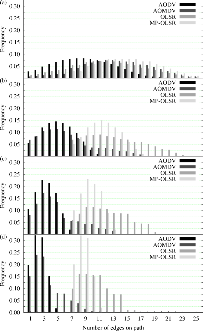
Figure 2: Distribution of path sizes for the original algorithms with $n=120$, for $\Delta=4$ (a), $\Delta=8$ (b), $\Delta=16$ (c), and $\Delta=32$ (d). For each value of $\Delta$ the distribution refers to $100$ networks and $100$ path sets per network, each corresponding to $n$ origin-destination pairs.

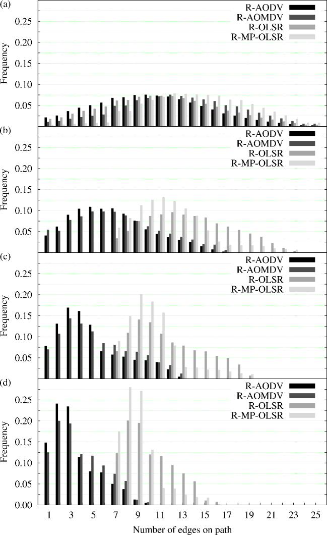
Figure 3: Distribution of path sizes for the refined algorithms with $n=120$, for $\Delta=4$ (a), $\Delta=8$ (b), $\Delta=16$ (c), and $\Delta=32$ (d). For each value of $\Delta$ the distribution refers to $100$ networks and $100$ path sets per network, each corresponding to $n$ origin-destination pairs.

4.2 Results

Our computational results relating to throughput are summarized in Fig. 4 for CBR1, Fig. 5 for CBR2, and Fig. 6 for SERA. Each figure is organized as a set of four panels, each for one of the four values of $\Delta$. All three figures show the behavior of the ratio, here denoted by $\sigma$, of each refined algorithm’s throughput to that of its original version. All plots are given against the ratio $\theta$ introduced earlier, which indicates what fraction of the $n$ origin-destination pairs corresponding to each path set is being taken into account. In all panels a highlighted horizontal line is used to mark the $\sigma=1$ threshold, above which a refined algorithm can be said to have overtaken its original version.

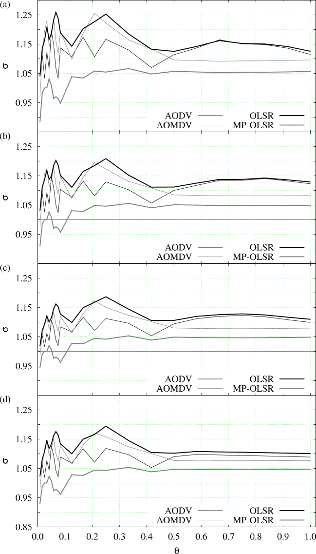
Figure 4: Throughput ratio for CBR1 with $n=120$, for $\Delta=4$ (a), $\Delta=8$ (b), $\Delta=16$ (c), and $\Delta=32$ (d). Data are averages over the $10^{4}$ path sets that correspond to each value of $\Delta$ for each value of $\theta$. Confidence intervals are less than $1\%$ of the mean at the $95\%$ level, so error bars are omitted.

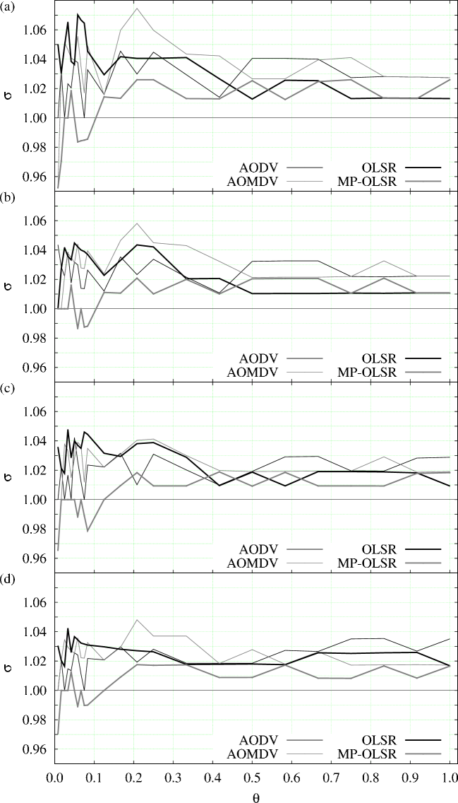
Figure 5: Throughput ratio for CBR2 with $n=120$, for $\Delta=4$ (a), $\Delta=8$ (b), $\Delta=16$ (c), and $\Delta=32$ (d). Data are averages over the $10^{4}$ path sets that correspond to each value of $\Delta$ for each value of $\theta$. Confidence intervals are less than $1\%$ of the mean at the $95\%$ level, so error bars are omitted.

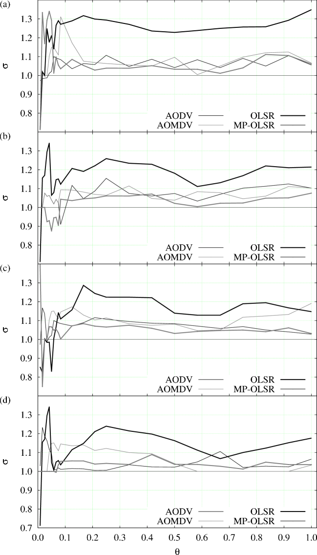
Figure 6: Throughput ratio for SERA with $n=120$, for $\Delta=4$ (a), $\Delta=8$ (b), $\Delta=16$ (c), and $\Delta=32$ (d). Data are averages over the $10^{4}$ path sets that correspond to each value of $\Delta$ for each value of $\theta$. Confidence intervals are less than $1\%$ of the mean at the $95\%$ level, so error bars are omitted.

Except for a few cases of $\theta<0.1$ (in which only a few origin-destination pairs coexist in the network and therefore refinement to achieve path-independence by noninterference is probably pointless to begin with), it follows from Figs. 4–6 that MRA was effective to some extent in all cases. Fixing the simulation scenario (CBR1, CBR2, or SERA) reveals that the behavior of $\sigma$ depends very little on the value of $\Delta$ or $\theta$ (provided $\theta$ is sufficiently large). Overall, the values of $\sigma$ seem best for the coupling of OLSR with SERA, followed by CBR1 coupled with either OLSR or MP-OLSR, and lastly for CBR2 without any marked preference for any routing method. Recall that the SERA scenario is TDMA-based, while both CBR1 and CBR2 are CSMA-based, with CBR1 operating at the higher rates.

Another perspective from which it is worth examining performance is that of fairness in the distribution of traffic through the paths. In other words, given an origin-destination pair and the multiple paths leading from the origin to the destination, we look at how traffic gets distributed through the various paths. One way of quantifying this is by means of the fairness index [24]. Given a set of paths $\mathcal{Q}$, the corresponding fairness index can be defined as $(\sum_{p\in\mathcal{Q}}x_{p})^{2}/|\mathcal{Q}|\sum_{p\in\mathcal{Q}}x_{p}^{2}$, where $x_{p}$ is the number of packets delivered to $j$ through path $p$ during the experiment. The fairness index ranges from $1/|\mathcal{Q}|$ to $1$, indicating when equal to $1$ that traffic is evenly distributed among the paths.

We give results on the fairness index in Figs. 7–9, respectively for CBR1, CBR2, and SERA. Note initially that, somewhat unexpectedly (owing to the algorithms’ markedly different strategies), AODV and OLSR are statistically indistinguishable from each other as far as fairness is concerned. The same holds for their refined versions, respectively R-AODV and R-OLSR. Note also that the fairness index, in all cases, tends to decrease as $\theta$ is increased. This means that, as might be expected, the presence of denser end-to-end traffic tends to disrupt the balance between paths more easily. AODV and OLSR have the best figures overall, better even than their refined versions. So, unlike throughput, fairness does not seem to improve as we extend a single-path algorithm’s set of paths and then apply MRA for refinement. All multi-path strategies, on the other hand, can be seen to benefit from the use of MRA.

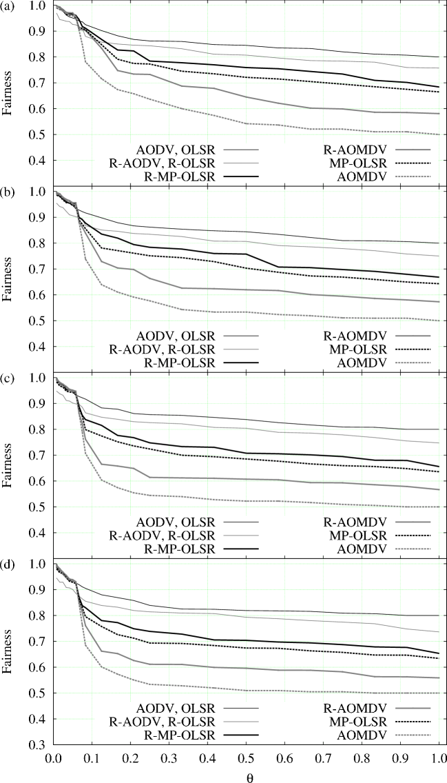
Figure 7: Fairness index for CBR1 with $n=120$, for $\Delta=4$ (a), $\Delta=8$ (b), $\Delta=16$ (c), and $\Delta=32$ (d). Data are averages over the $10^{4}$ path sets that correspond to each value of $\Delta$ for each value of $\theta$. Confidence intervals are less than $1\%$ of the mean at the $95\%$ level, so error bars are omitted.

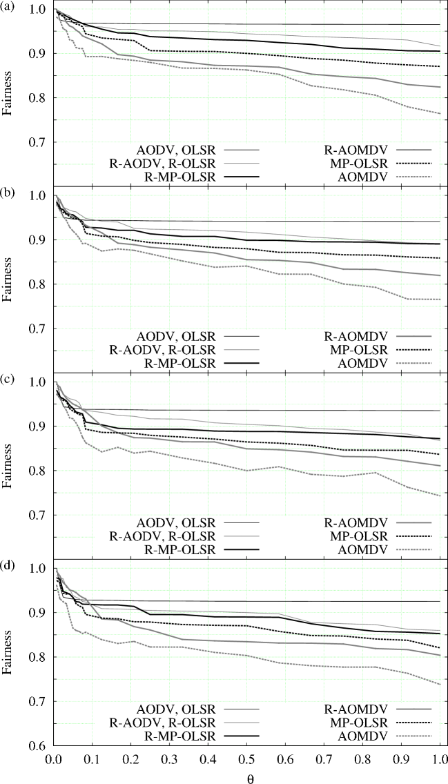
Figure 8: Fairness index for CBR2 with $n=120$, for $\Delta=4$ (a), $\Delta=8$ (b), $\Delta=16$ (c), and $\Delta=32$ (d). Data are averages over the $10^{4}$ path sets that correspond to each value of $\Delta$ for each value of $\theta$. Confidence intervals are less than $1\%$ of the mean at the $95\%$ level, so error bars are omitted.

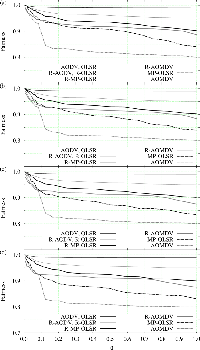
Figure 9: Fairness index for SERA with $n=120$, for $\Delta=4$ (a), $\Delta=8$ (b), $\Delta=16$ (c), and $\Delta=32$ (d). Data are averages over the $10^{4}$ path sets that correspond to each value of $\Delta$ for each value of $\theta$. Confidence intervals are less than $1\%$ of the mean at the $95\%$ level, so error bars are omitted.

Another interesting trend that can be observed in Figs. 7–9 is that, though always decaying with $\theta$ as we noted, in general the fairness index is best for SERA, followed by CBR2, then by CBR1. While we believe the position of SERA in this rank to be closely related to its TDMA-based nature, it is curious to observe that the relative positions of CBR1 and CBR2 are exchanged with respect to what we observed for throughput. It seems, then, that in selecting between the rates associated with CBR1 and CBR2 one is automatically forced to favor throughput over fairness or conversely.

Our definition of the fairness index given above is only one of the possibilities in the context of multi-path routing. Another alternative is to coalesce all packets delivered from one origin, say $i$, to one destination, say $j$, into a single number $x_{ij}$ and then compute the fairness index as $(\sum_{ij\in OD}x_{ij})^{2}/|OD|\sum_{ij\in OD}x_{ij}^{2}$. Proceeding in this way would shift the focus of the fairness index from paths to origin-destination pairs. We give no detailed results on this alternative, but do provide an example with SERA in Fig. A.4. There is clearly great similarity with the results in Fig. 9, but the numbers tend to be higher.

5 Discussion

As we remarked earlier, we have provided no results for $n\in\{60,80,100\}$ because, essentially, they are indistinguishable from those of $n=120$ in qualitative terms. We do remark, however, that a few noteworthy quantitative differences were observed. For example, in the case of SERA a higher throughput ratio $\sigma$ was sometimes observed for reduced $n$ but the same value of the pair density $\theta$. This stems not only from the fact that the average path size decreases as $n$ decreases, but more generally from the fact that the number of links for the same $\theta$ is lower in the smaller networks, thus fewer links interfere with one another and fewer links have to be scheduled. Such improvement in the value of $\sigma$, therefore, seems to depend on the network’s path-size distribution.

As we noted briefly in Section 4.2, often OLSR and MP-OLSR turned out to be the routing methods most prone to benefit from the refinement provided by MRA. One clue as to why this is so may be already present in Table 3, where the refined versions of these two methods have some of the lowest path multiplicities overall, thence a tendency to incur less interference. However, this holds also for the refined version of AODV, so there has to be some other distinguishing aspect. While our data are not sufficient to provide a definitive answer, we believe the two methods’ superiority to be owed to a combination of MRA (which attempts to reduce path multiplicity to lower interference) with the MPR concept that is intrinsic to the OLSR variants (which in turn attempts to provide an initial set of paths as spatially distributed as possible). As for AODV, the SPA at its core probably produces paths that are less spatially separated [55, 10].

In a related vein, the results of Section 4.2 also point at SERA as providing superior throughput results vis-à-vis those of CBR1 and CBR2, and similarly for CBR1 with respect to CBR2. Because such results refer to throughput gains after refinement by MRA, more detailed data are needed for a direct comparison of throughputs. These are shown in Figs. A.5–A.7, which clearly confirm the rank. Once again the reason for this is not totally clear, but it may be a manifestation of SERA’s properties rather than of the superiority of its underlying TDMA scheme over the CSMA protocols of CBR1 and CBR2. After all, a considerable amount of research has been directed toward the TDMA versus CSMA question, without however reaching an agreement [16, 20, 15, 9].

Another curiosity related to this issue of how SERA compares to CBR1 and CBR2 has to do with the total absence of traffic on some paths. While SERA precludes this from occurring as a matter of design principle, unused paths do occur in the other two cases. During the corresponding NS2 simulations this persisted even if simulation times were extended or the synchronization of multiple CBRs was reordered or entirely removed. As it turns out, it seems that certain paths remained unused so that throughput could be increased on other paths. Data on the most critical cases, viz. those in which no packets at all were delivered for an origin-destination pair, are shown in Figs. A.8 and A.9. Examining these data confirms our expectation that the single-path algorithms should be less prone to the occurrence of such extreme cases. It also reveals that both R-AOMDV and R-MP-OLSR had fewer such occurrences than their corresponding originals (i.e., MRA seems to have attenuated the problem).

6 Concluding remarks

MRA is a heuristic for the refinement of routing paths in WMNs. It was developed with multi-path routing algorithms in mind but works also on single-path algorithms (through a manipulation of its input to obtain multiple paths from the overall set of single paths). MRA is fully local, in the sense that it depends only on information that is readily available to each node and its immediate neighborhood in the network. Being local means that the extra control traffic it may entail is negligible, especially if we consider that it need happen only once for a fixed set of paths. It involves the solution of an NP-hard problem, that of finding a maximum weighted independent set in a graph, but the inputs involved are typically very small, leading to negligible running times if compared to arbitrary graphs [36].

Our computational experiments with MRA on a TDMA setting (SERA) and two CSMA settings (CBR1 and CBR2) revealed improvements in throughput of up to $30\%$ for both the AODV and OLSR routing methods and their multi-path variants. The latter were also improved by MRA in terms of fairness. Finding out just how close these improvements come to the very best that can be achieved is an open problem that involves solving the path-pruning problem globally. This problem is NP-hard as the one solved by MRA, but its input, relating to the WMN in a global scale, is much more sizable.

Another interesting aspect for further investigation is the effect of MRA on multi-radio networks. In such schemes the network’s path density can be drastically reduced for a given frequency, thus potentially benefiting MRA. Conversely, it may also be possible to use MRA to achieve the desirable goal of minimizing the number of radios [6, 39]. Further research is also needed on the trade-off that clearly exists between obtaining spatially separated paths or relatively short ones. While the former is good for non-interference, disregarding the latter may lead to throughput loss on the relatively longer paths.

Appendix A Supplementary figures

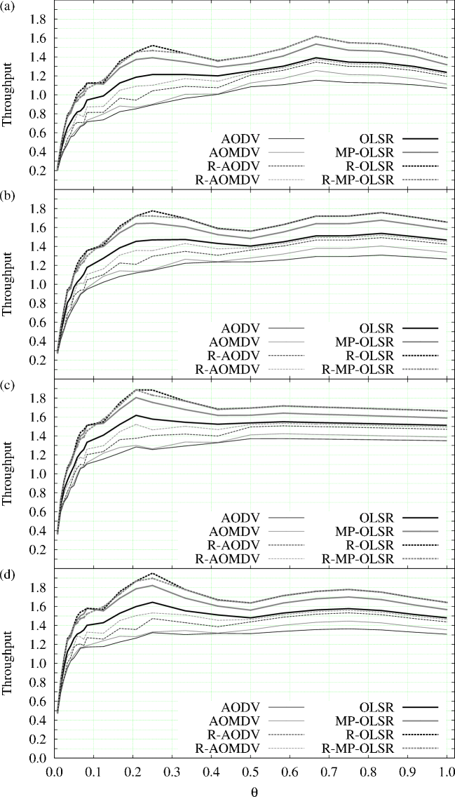
Figure A.1: Throughput (packets/time slot) for CBR1 with $n=120$, for $\Delta=4$ (a), $\Delta=8$ (b), $\Delta=16$ (c), and $\Delta=32$ (d). Data are averages over the $10^{4}$ path sets that correspond to each value of $\Delta$ for each value of $\theta$. Confidence intervals are less than $1\%$ of the mean at the $95\%$ level, so error bars are omitted.

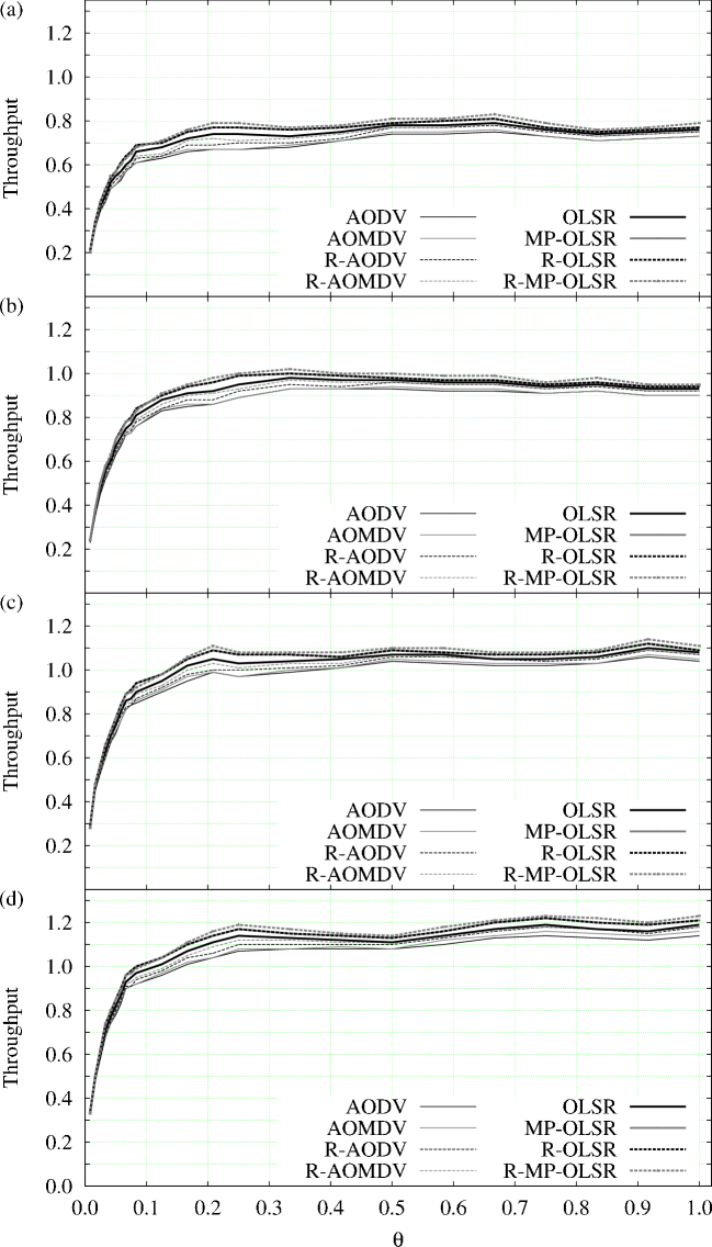
Figure A.2: Throughput (packets/time slot) for CBR2 with $n=120$, for $\Delta=4$ (a), $\Delta=8$ (b), $\Delta=16$ (c), and $\Delta=32$ (d). Data are averages over the $10^{4}$ path sets that correspond to each value of $\Delta$ for each value of $\theta$. Confidence intervals are less than $1\%$ of the mean at the $95\%$ level, so error bars are omitted.

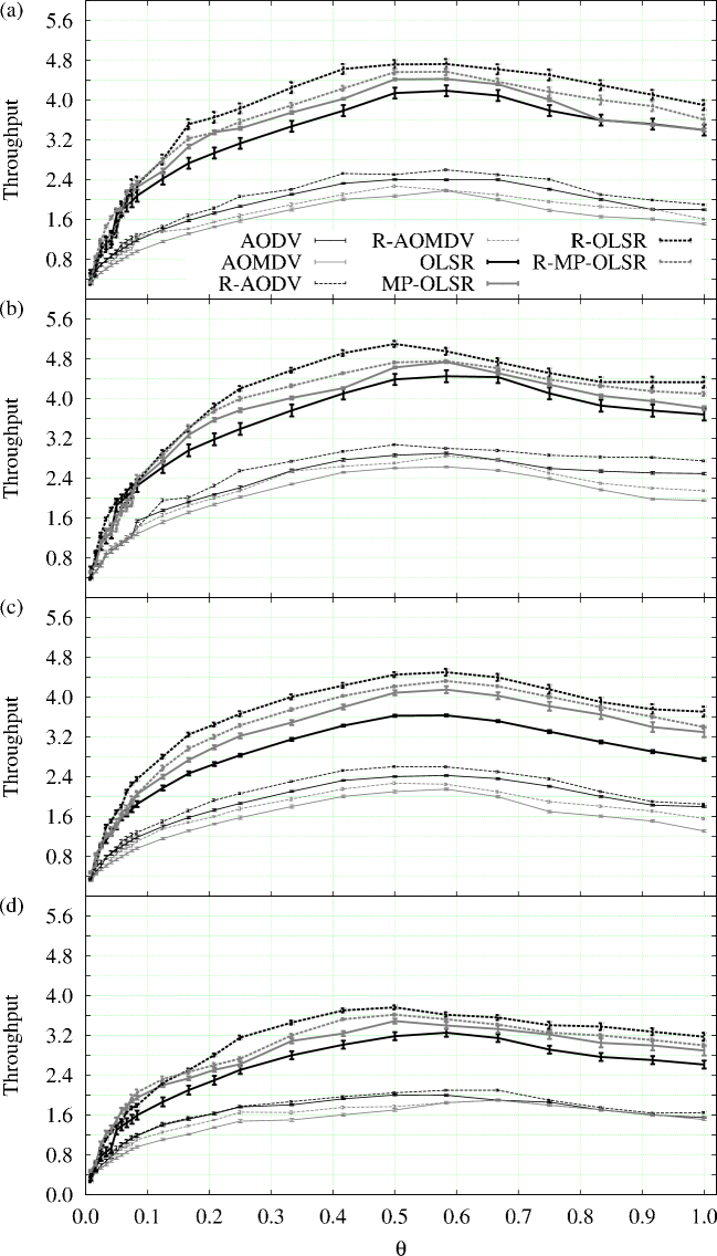
Figure A.3: Throughput (packets/time slot) for SERA with $n=120$, for $\Delta=4$ (a), $\Delta=8$ (b), $\Delta=16$ (c), and $\Delta=32$ (d). Data are averages over the $10^{4}$ path sets that correspond to each value of $\Delta$ for each value of $\theta$. Error bars are based on confidence intervals at the $95\%$ level.

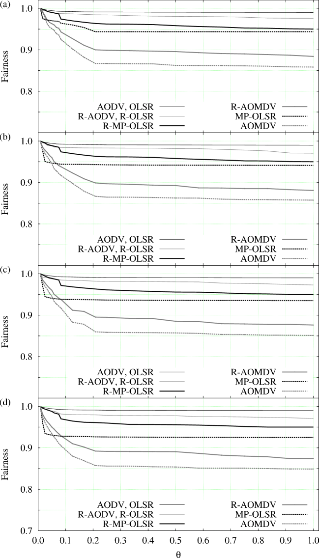
Figure A.4: Alternative fairness index for SERA with $n=120$, for $\Delta=4$ (a), $\Delta=8$ (b), $\Delta=16$ (c), and $\Delta=32$ (d). Data are averages over the $10^{4}$ path sets that correspond to each value of $\Delta$ for each value of $\theta$. Confidence intervals are less than $1\%$ of the mean at the $95\%$ level, so error bars are omitted.

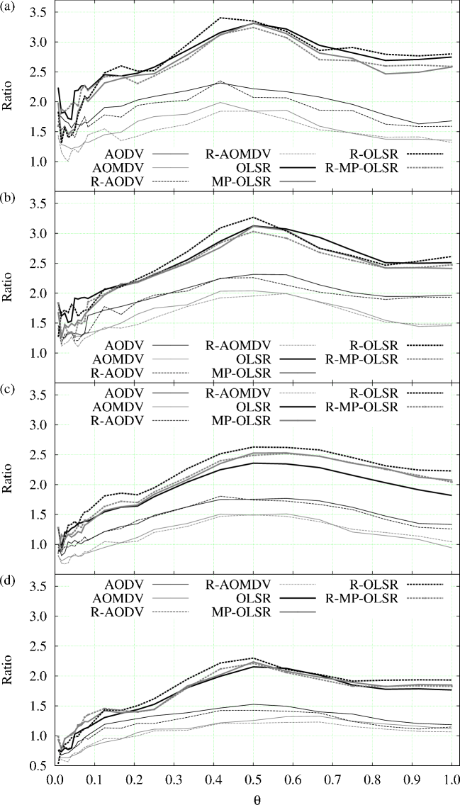
Figure A.5: Ratio of SERA’s throughput to that of CBR1 with $n=120$, for $\Delta=4$ (a), $\Delta=8$ (b), $\Delta=16$ (c), and $\Delta=32$ (d). Data are averages over the $10^{4}$ path sets that correspond to each value of $\Delta$ for each value of $\theta$. Confidence intervals are less than $1\%$ of the mean at the $95\%$ level, so error bars are omitted.

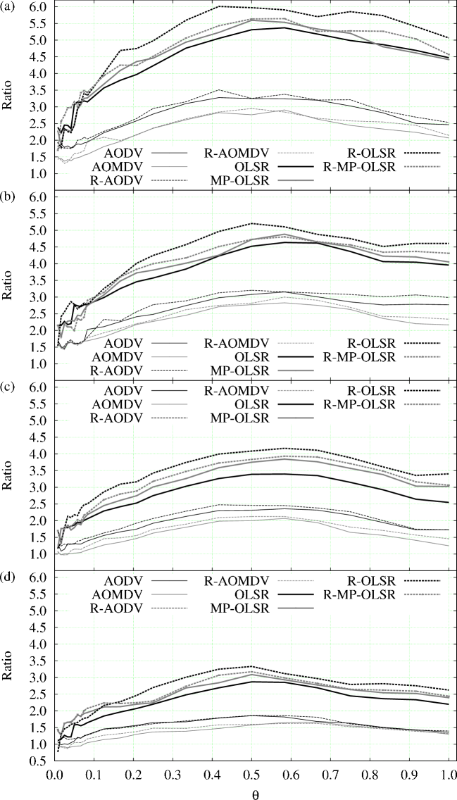
Figure A.6: Ratio of SERA’s throughput to that of CBR2 with $n=120$, for $\Delta=4$ (a), $\Delta=8$ (b), $\Delta=16$ (c), and $\Delta=32$ (d). Data are averages over the $10^{4}$ path sets that correspond to each value of $\Delta$ for each value of $\theta$. Confidence intervals are less than $1\%$ of the mean at the $95\%$ level, so error bars are omitted.

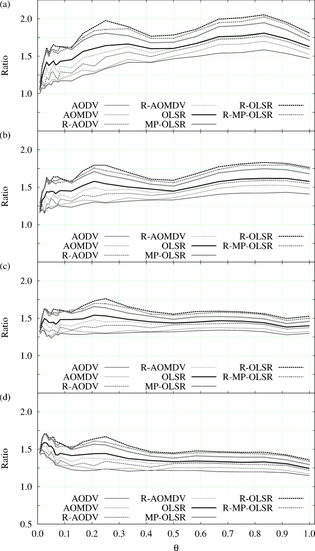
Figure A.7: Ratio of CBR1’s throughput to that of CBR2 with $n=120$, for $\Delta=4$ (a), $\Delta=8$ (b), $\Delta=16$ (c), and $\Delta=32$ (d). Data are averages over the $10^{4}$ path sets that correspond to each value of $\Delta$ for each value of $\theta$. Confidence intervals are less than $1\%$ of the mean at the $95\%$ level, so error bars are omitted.

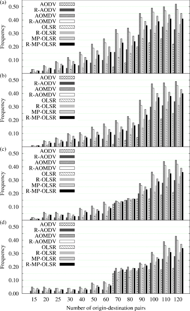
Figure A.8: Distribution of the number of origin-destination pairs without any traffic in CBR1 with $n=120$, for $\Delta=4$ (a), $\Delta=8$ (b), $\Delta=16$ (c), and $\Delta=32$ (d). Data are averages over the $10^{4}$ path sets that correspond to each value of $\Delta$.

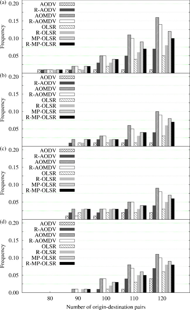
Figure A.9: Distribution of the number of origin-destination pairs without any traffic in CBR2 with $n=120$, for $\Delta=4$ (a), $\Delta=8$ (b), $\Delta=16$ (c), and $\Delta=32$ (d). Data are averages over the $10^{4}$ path sets that correspond to each value of $\Delta$.

References

- [1] M. Abolhasan. A review of routing protocols for mobile ad hoc networks. Ad Hoc Netw., 2:1–22, 2004.
- [2] I. F. Akyildiz, X. Wang, and W. Wang. Wireless mesh networks: a survey. Comput. Netw., 47:445–487, 2005.
- [3] M. Alicherry, R. Bhatia, and L. E. Li. Joint channel assignment and routing for throughput optimization in multiradio wireless mesh networks. IEEE J. Sel. Area Commun., 24:1960–1971, 2006.
- [4] C. H. P. Augusto, C. B. Carvalho, M. W. R. da Silva, and J. F. de Rezende. REUSE: a combined routing and link scheduling mechanism for wireless mesh networks. Comput. Commun., 34:2207–2216, 2011.
- [5] C. H. P. Augusto, C. B. Carvalho, M. W. R. Silva, and J. F. de Rezende. The impact of joint routing and link scheduling on the performance of wireless mesh networks. In Proceedings of the IEEE LCN 2010, pages 80–87, 2010.
- [6] P. Bahl, A. Adya, J. Padhye, and A. Walman. Reconsidering wireless systems with multiple radios. Comput. Commun. Rev., 34:39–46, October 2004.
- [7] A. Balachandran, G. M. Voelker, and P. Bahl. Wireless hotspots: current challenges and future directions. Mob. Netw. Appl., 10:265–274, 2005.
- [8] H. Balakrishnan, C. L. Barrett, V. S. A. Kumar, M. V. Marathe, and S. Thite. The distance-2 matching problem and its relationship to the MAC-layer capacity of ad hoc wireless networks. IEEE J. Sel. Area Commun., 22:1069–1079, 2004.
- [9] S. Banaouas and P. Muhlethaler. Performance evaluation of TDMA versus CSMA-based protocols in SINR models. In Proceedings of the EW 2009, pages 113–117, 2009.
- [10] S. R. Biradar, K. Majumder, S. K. Sarkar, and Puttamadappa C. Performance evaluation and comparison of AODV and AOMDV. Int. J. Comput. Sci. Eng., 2:373–377, 2010.
- [11] M. E. M. Campista, P. M. Esposito, I. M. Moraes, L. H. M. Costa, O. C. M. Duarte, D. G. Passos, C. V. N. Albuquerque, D. C. M. Saade, and M. G. Rubinstein. Routing metrics and protocols for wireless mesh networks. IEEE Netw., 22:6–12, January 2008.
- [12] Y. Chun, L. Qin, L. Yong, and S. MeiLin. Routing protocols overview and design issues for self-organized network. In Proceedings of the WCC ICCT 2000, pages 1298–1303, 2000.
- [13] R. L. Cruz and A. V. Santhanam. Optimal routing, link scheduling and power control in multihop wireless networks. In Proceedings of the IEEE INFOCOM 2003, pages 702–711, 2003.
- [14] I. Demirkol, C. Ersoy, and F. Alagoz. MAC protocols for wireless sensor networks: a survey. IEEE Commun. Mag., 44:115–121, April 2006.
- [15] A. Dhekne, N. Uchat, and B. Raman. Implementation and evaluation of a TDMA MAC for WiFi-based rural mesh networks. In Proceedings of the NSDR 2009, 2009.
- [16] J. Ding, L. Zhao, S. R. Medidi, and K. M. Sivalingam. MAC protocols for Ultra-Wide-Band (UWB) wireless networks: impact of channel acquisition time. In Proceedings of the SPIE ITCOM 2002, pages 1953–1954, 2002.
- [17] G. A. Dirac. Some theorems on abstract graphs. Proc. Lond. Math. Soc., s3-2:69–81, 1952.
- [18] A. Gotta, F. Potorti, and R. Secchi. Simulating dynamic bandwidth allocation on satellite links. In Proceeding of the WNS2 2006, pages 8–17, 2006.
- [19] A. Chandra V. Gummalla and J. O. Limb. Wireless medium access control protocols. IEEE Commun. Surv. Tutor., 3:2–15, Second Quarter 2000.
- [20] G. P. Gupta and A. K. Pandey. Performance comparison of ad hoc routing protocols over IEEE 802.11 DCF and TDMA MAC layer protocols. In Proceedings of the NCC 2007, pages 183–187, 2007.
- [21] P. Gupta and P. R. Kumar. The capacity of wireless networks. IEEE Trans. Inf. Theory, 46:388–404, 2000.
- [22] A. J. Hoffman. On the polynomial of a graph. Am. Math. Month., 70:30–36, 1963.
- [23] P. Jacquet, P. Muhlethaler, T. Clausen, A. Laouiti, A. Qayyum, and L. Viennot. Optimized link state routing protocol for ad hoc networks. In Proceedings of the IEEE INMIC 2001, pages 62–68, 2001.
- [24] R. Jain, D.-M. Chiu, and W. Hawe. A quantitative measure of fairness and discrimination for resource allocation in shared computer systems. http://arxiv.org/abs/cs.NI/9809099, 1998.
- [25] T.-S. Kim, H. Lim, and J. C. Hou. Improving spatial reuse through tuning transmit power, carrier sense threshold, and data rate in multihop wireless networks. In Proceedings of the MobiCom 2006, pages 366–377, 2006.
- [26] S. Ktari, H. Labiod, and M. Frikha. Load balanced multipath routing in mobile ad hoc network. In Proceedings of the IEEE ICCS 2006, pages 1–5, 2006.
- [27] S. J. Lee and M. Gerla. Split multipath routing with maximally disjoint paths in ad hoc networks. In Proceedings of the IEEE ICC 2001, pages 3201–3205, 2001.
- [28] S.-J. Lee, W. Su, and M. Gerla. Wireless ad hoc multicast routing with mobility prediction. Mob. Netw. Appl., 6:351–360, 2001.
- [29] X. Li and L. Cuthbert. On-demand node-disjoint multipath routing in wireless ad hoc networks. In Proceedings of the IEEE LCN 2004, pages 419–420, 2004.
- [30] X. Lin and S. Rasool. A distributed joint channel-assignment, scheduling and routing algorithm for multi-channel ad-hoc wireless networks. In Proceedings of the INFOCOM 2007, pages 1118–1126, 2007.
- [31] M. K. Marina and S. R. Das. Ad hoc on-demand multipath distance vector routing. Mob. Comput. Commun. Rev., 6:92–93, July 2002.
- [32] MP-OLSR routing agent for NS-2. http://jiaziyi.com/MP-OLSR.php, 2008.
- [33] N. Nandiraju, D. Nandiraju, L. Santhanam, B. He, J. Wang, and D. P. Agrawal. Wireless mesh networks: current challenges and future directions of web-in-the-sky. IEEE Wirel. Commun., 14:79–89, August 2007.
- [34] NO Ad-Hoc routing agent (NOAH). http://icapeople.epfl.ch/widmer/uwb/ns-2/noah/, 2004.
- [35] The network simulator NS-2. http://www.isi.edu/nsnam/ns/, 1989.
- [36] P. M. Pardalos and N. Desai. An algorithm for finding a maximum weighted independent set in an arbitrary graph. J. Comput. Math., 38:163–175, 1991.
- [37] M. R. Pearlman, Z. J. Haas, P. Sholander, and S. S. Tabrizi. On the impact of alternate path routing for load balancing in mobile ad hoc networks. In Proceedings of the MobiHoc 2000, pages 3–10, 2000.
- [38] C. E. Perkins and E. M. Royer. Ad-hoc on-demand distance vector routing. In Proceedings of the WMCSA 1999, pages 90–100, 1999.
- [39] A. Raniwala and T.-C. Chiueh. Architecture and algorithms for an IEEE 802.11-based multi-channel wireless mesh network. In Proceedings of the IEEE INFOCOM 2005, pages 2223–2234, 2005.
- [40] I. Rhee, A. Warrier, J. Min, and L. Xu. DRAND: distributed randomized TDMA scheduling for wireless ad-hoc networks. In Proceedings of the MobiHoc 2006, pages 190–201, 2006.
- [41] I. Sheriff and E. Belding Royer. Multipath selection in multi-radio mesh networks. In Proceedings of the BROADNETS 2006, pages 1–11, 2006.
- [42] Y. Shi, Y. T. Hou, J. Liu, and S. Kompella. How to correctly use the protocol interference model for multi-hop wireless networks. In Proceedings of the MobiHoc 2009, pages 239–248, 2009.
- [43] M. Siekkinen, V. Goebel, T. Plagemann, K.-A. Skevik, M. Banfield, and I. Brusic. Beyond the future Internet—requirements of autonomic networking architectures to address long term future networking challenges. In Proceedings of the FTDCS 2007, pages 89–98, 2007.
- [44] V. Srikanth, A. C. Jeevan, B. Avinash, T. S. Kiran, and S. S. Babu. A review of routing protocols in wireless mesh networks. Int. J. Comput. Appl., 1:47–51, 2010.
- [45] M. Tarique, K. E. Tepe, S. Adibi, and S. Erfani. Survey of multipath routing protocols for mobile ad hoc networks. J. Netw. Comput. Appl., 32:1125–1143, 2009.
- [46] J. Tsai and T. Moors. A review of multipath routing protocols: from wireless ad hoc to mesh networks. http://citeseerx.ist.psu.edu/viewdoc/download?doi=10.1.1.84.5817&rep=rep1&type=pdf, 2006.
- [47] A. Tsirigos and Z. J. Haas. Multipath routing in the presence of frequent topological changes. IEEE Commun. Mag., 39:132–138, November 2001.
- [48] F. R. J. Vieira, J. F. de Rezende, V. C. Barbosa, and S. Fdida. Scheduling links for heavy traffic on interfering routes in wireless mesh networks. Comput. Netw., 2012. To appear.
- [49] S. Waharte and R. Boutaba. Totally disjoint multipath routing in multihop wireless networks. In Proceedings of the IEEE ICC 2006, pages 5576–5581, 2006.
- [50] S. Waharte and R. Boutaba. On the probability of finding non-interfering paths in wireless multihop networks. In Proceedings of the IFIP TC6 2008, volume 4982 of Lecture Notes in Computer Science, pages 914–921, Berlin, Germany, 2008. Springer.
- [51] J. Wang, P. Du, W. Jia, L. Huang, and H. Li. Joint bandwidth allocation, element assignment and scheduling for wireless mesh networks with MIMO links. Comput. Commun., 31:1372–1384, 2008.
- [52] W. Wang, Y. Wang, X.-Y. Li, W.-Z. Song, and O. Frieder. Efficient interference-aware TDMA link scheduling for static wireless networks. In Proceedings of the MobiCom 2006, pages 262–273, 2006.
- [53] X. Wang and J. J. Garcia-Luna-Aceves. Embracing interference in ad hoc networks using joint routing and scheduling with multiple packet reception. Ad Hoc Netw., 7:460–471, 2009.
- [54] J. Yi, A. Adnane, S. David, and B. Parrein. Multipath optimized link state routing for mobile ad hoc networks. Ad Hoc Netw., 9:28–47, 2011.
- [55] J. Yi, E. Cizeron, S. Hamma, and B. Parrein. Simulation and performance analysis of MP-OLSR for mobile ad hoc networks. In Proceedings of the IEEE WCNC 2008, pages 2235–2240, 2008.
- [56] Y. Yuan, H. Chen, and M. Jia. An optimized Ad-hoc On-demand Multipath Distance Vector (AOMDV) routing protocol. In Proceedings of the APCC 2005, pages 569–573, 2005.
- [57] X. Zhou, Y. Lu, and B. Xi. A novel routing protocol for ad hoc sensor networks using multiple disjoint paths. In Proceedings of the BROADNETS 2005, pages 944–948, 2005.