On image segmentation using information theoretic criteria

Abstract

Image segmentation is a long-studied and important problem in image processing. Different solutions have been proposed, many of which follow the information theoretic paradigm. While these information theoretic segmentation methods often produce excellent empirical results, their theoretical properties are still largely unknown. The main goal of this paper is to conduct a rigorous theoretical study into the statistical consistency properties of such methods. To be more specific, this paper investigates if these methods can accurately recover the true number of segments together with their true boundaries in the image as the number of pixels tends to infinity. Our theoretical results show that both the Bayesian information criterion (BIC) and the minimum description length (MDL) principle can be applied to derive statistically consistent segmentation methods, while the same is not true for the Akaike information criterion (AIC). Numerical experiments were conducted to illustrate and support our theoretical findings.

and

t1Supported in part by NSF Grant 0905400. t2Supported in part by NSF Grants 0707037 and 1007520.

1 Introduction

Image segmentation aims to partition an image into a set of nonoverlapping regions so that pixels within the same region are homogeneous with respect to some characteristic (e.g., gray value or roughness), while pixels from adjacent regions are significantly different with respect to the same characteristic. It is a fundamental problem in image processing, as very often it is necessary to first group the highly localized pixels into more global and meaningful segmented objects to facilitate the extraction of useful information. In this paper, gray value is the image characteristic that forms the basis for segmentation. For general introductions to image segmentation, see, for example, Glasbey and Horgan (1995) and Haralick and Shapiro (1992).

A grayscale image can be seen as a two-dimensional (2D) surface living in a three-dimensional space. Therefore one popular approach to segmenting it is to model it by a 2D piecewise constant function, with the set of all discontinuity points defining the region boundaries of the image. Examples of segmentation methods that follow this approach include Kanungo et al. (1995), LaValle and Hutchinson (1995), Leclerc (1989), Lee (1998, 2000), Luo and Khoshgoftaar (2006) and Wang, Ju and Wang (2009). As to be demonstrated below, segmenting images with this approach can be recast as a model selection problem, and one crucial issue to its success is the choice of the model complexity, which is equaivalent to choosing the number of regions together with the shapes of their boundaries. Common information theoretic methods such as the Akaike information criterion (AIC) [Akaike (1974)], the Bayesian information criterion (BIC), also known as the Schwarz information criterion [Schwarz (1978)] and the minimum description length (MDL) principle [Rissanen (1989, 2007)] have been adopted to solve this problem; for example, see Kanungo et al. (1995), Leclerc (1989), Lee (1998, 2000), Luo and Khoshgoftaar (2006), Murtagh, Raftery and Starck (2005), Stanford and Raftery (2002), Zhang and Modestino (1990) and Zhu and Yuille (1996). While many of these methods produce excellent practical results, their theoretical properties are still largely unknown. The goal of this paper is to conduct a systematic study on the theoretical properties of these methods, with the hope of enhancing our understanding of their performances, at both theoretical and empirical levels. To the best of our knowledge, this is the first time that such a rigorous theoretical study is being performed for image segmentation methods.

The rest of this paper is organized as follows. Background material is presented in Section 2. Section 3 presents our main theoretical results. These theoretical results are empirically verified by numerical experiments in Section 4. Concluding remarks are offered in Section 6, while technical details are delayed to the Appendix.

2 Background

Denote by $f$ the true image and $\Xi_{n}=\{x_{1},\ldots,x_{n}\}$ the set of $n$ grid points at which a noisy version of $f$ is sampled. Without loss of generality it is assumed that the domain of $f$ is $[0,1]^{2}$. As mentioned before, $f$ is modeled as a 2D piecewise constant function as follows. Write $f_{i}=f(x_{i})$ and $\mathbf{f}=(f_{1},\ldots,f_{n})^{\prime}$. Let the number of regions (or pieces or segments) in $f$ be $m$, and denote the gray value and domain of the $\nu$th region as $\mu_{\nu}$ and $R_{\nu}$, respectively. Then we have, for $i=1,\ldots,n$,

$$f_{i} = \mu_{\nu}\qquad\mbox{if }x_{i}\in R_{\nu},$$ (1)

$$\bigcup_{\nu=1}^{m}R_{\nu} = [0,1]^{2}\quad\mbox{and}\quad R_{\nu}\cap R_{\nu^{\prime}}=\varnothing\qquad\mbox{if }\nu\not=\nu^{\prime}.$$ (2)

In the sequel we write $\mathbf{R}=(R_{1},\ldots,R_{m})$ and ${\bolds{\mu}}=(\mu_{1},\ldots,\mu_{m})^{\prime}$. Thus $\mathbf{R}$ defines a segmentation of $f$. The observed noisy version $\mathbf{y}=(y_{1},\ldots,y_{n})^{\prime}$ of $\mathbf{f}$ is modeled as

$$y_{i}=f_{i}+\varepsilon_{i},\qquad i=1,\ldots,n,$$ (3)

where the noise $\varepsilon_{i}$’s are independent, identically distributed random variables with zero mean and variance $\sigma^{2}$. Given $\mathbf{y}$, the goal is then to estimate $\mathbf{f}$, which is equivalent to estimating $m$, $\mathbf{R}$ and ${\bolds{\mu}}$.

For simplicity, denote by ${\bolds\theta}_{m}=(m,\mathbf{R},{\bolds{\mu}})^{\prime}$ a generic parameter vector. Estimating $\mathbf{f}$ is hence equivalent to the model selection problem in which each model is determined by the parameter ${\bolds\theta}_{m}$. Let $\mathrm{RSS}_{m}=\sum_{i}(y_{i}-\hat{f}_{i})^{2}$ be the corresponding residual sum of squares. Notice that different values of $m$ would lead to a different number of parameters in ${\bolds\theta}_{m}$. Also notice that ${\bolds\theta}_{m}$ cannot be estimated by minimizing $\mathrm{RSS}_{m}$, as $\mathrm{RSS}_{m}$ can be made arbitrarily small as $m$ tends to $n$. One way to resolve this issue is to add a penalty term to $\mathrm{RSS}_{m}$ to suitably penalize the complexity of ${\bolds\theta}_{m}$. As alluded to before, information theoretic model selection methods like AIC, BIC and MDL can be used to derive such a penalty. We first focus on the MDL criterion derived by Lee (2000),

$$\operatorname{MDL}(m,\mathbf{R})=m\ln n+\frac{\ln 3}{2}\sum_{\nu=1}^{m}b_{\nu}+\frac{1}{2}\sum_{\nu=1}^{m}\ln a_{\nu}+\frac{n}{2}\ln\biggl{(}\frac{\mathrm{RSS}_{m}}{n}\biggr{)},$$ (4)

where each region $R_{\nu}$ enters through its “area” $a_{\nu}$ (in terms of number of pixels) and “perimeter” $b_{\nu}$ (in terms of number of pixel edges). These quantities are formally defined as

$$a_{\nu}=\#(\Xi_{n}\cap R_{\nu})\quad\mbox{and}\quad b_{\nu}=\#(\Xi_{n}\cap\partial R_{\nu})$$

with $\#A$ and $\partial A$ indicating, respectively, cardinality and boundary of the set $A$. Observe that, once the estimates $\hat{m}$ and $\hat{\mathbf{R}}$ are specified, ${\bolds{\mu}}$ can be uniquely estimated by

$$\hat{\mu}_{\nu}=\frac{1}{\hat{a}_{\nu}}\sum_{i\in\hat{R}_{\nu}}y_{i}\qquad\mbox{for all $\nu$},$$ (5)

and therefore ${\bolds{\mu}}$ is dropped in the argument list of $\operatorname{MDL}(m,\mathbf{R})$. To sum up, the MDL-based method of Lee (2000) estimates $m$ and $\mathbf{R}$ as the joint minimizer of (4), which is equivalent to saying

$$(\hat{m},\hat{\mathbf{R}})=\mathop{\arg\min}_{m\leq M,\mathbf{R}}\frac{2}{n}\operatorname{MDL}(m,\mathbf{R}),$$ (6)

and $\hat{{\bolds{\mu}}}$ is given by (5). Practical algorithms, developed, for example, by Lee (2000) and Zhu and Yuille (1996), can be used to solve (6).

One can also use AIC and BIC to derive penalty terms to add to $\mbox{RSS}_{m}$, and the resulting penalties will be proportional to the number of “free” (and independent) parameters in the fitted image $\hat{\mathbf{f}}$ [e.g., Murtagh, Raftery and Starck (2005), Stanford and Raftery (2002) and Zhang and Modestino (1990)]. This leads to the following question: what would be a meaningful way of counting the number of free parameters in $\hat{\mathbf{f}}$? There seems to be no unique answer, but we shall follow Murtagh, Raftery and Starck (2005) and Stanford and Raftery (2002) and model each true pixel value $f_{i}$ with a mixture distribution of $m$ Gaussians, where the mean, variance and mixing probability for the $\nu$th Gaussian are $\mu_{\nu}$, $\sigma^{2}$ and $a_{\nu}/\sum_{\nu}a_{\nu}$, respectively. As there are $m$ of the $\mu_{\nu}$’s, one $\sigma^{2}$ and $m-1$ free mixing probabilities, the total number of free parameters is $2m$. With this, the corresponding AIC and BIC segmentation criteria are

$$\operatorname{AIC}(m,\mathbf{R})=2m+\frac{n}{2}\ln\biggl{(}\frac{\mathrm{RSS}_{m}}{n}\biggr{)}$$

and

$$\operatorname{BIC}(m,\mathbf{R})=m\ln n+\frac{n}{2}\ln\biggl{(}\frac{\mathrm{RSS}_{m}}{n}\biggr{)},$$

respectively. The AIC and BIC estimates for $(m,\mathbf{R})$ are then given by

$$(\hat{m},\hat{\mathbf{R}})=\mathop{\arg\min}_{m\leq M,\mathbf{R}}\frac{2}{n}\operatorname{AIC}(m,\mathbf{R})$$ (7)

and

$$(\hat{m},\hat{\mathbf{R}})=\mathop{\arg\min}_{m\leq M,\mathbf{R}}\frac{2}{n}\operatorname{BIC}(m,\mathbf{R}),$$ (8)

respectively. Observe that for both $\operatorname{AIC}(m,\mathbf{R})$ and $\operatorname{BIC}(m,\mathbf{R})$, the region boundaries $\mathbf{R}$ are not explicitly penalized; they enter the criteria only through $\mbox{RSS}_{m}$. Also observe that the penalty term of $\operatorname{AIC}(m,\mathbf{R})$ is independent of $n$.

Before we proceed further, it is worthwhile to point out a major difference between the variable selection problem in linear regression models and the image segmentation problem. In variable selection for linear regression, the goal is to select the significant predictors and remove the insignificant ones from the model. In other words, some “data” are not used in estimating the model parameters. For image segmentation, the goal is to group homogeneous pixels together to form segmented objects, and in this process all data (i.e., all pixel values) are always used to estimate the model parameters. Given this major difference, one can see that variable selection in linear regression and image segmentation are two different problems, and hence existing theories from classical linear regression modeling cannot be directly applied to image segmentation.

3 Main results

This section presents our main theoretical findings. Briefly, both the BIC and MDL segmentation solutions are statistically consistent in a well-defined sense, while the AIC solution is not.

The consistency of the BIC and MDL solutions are investigated at two levels. First, we will establish the strong consistency of $\hat{\mathbf{R}}$ if the true number of regions $m=m^{0}$ can be assumed known. Second, if the true value $m^{0}$ is unknown and if the noise is restricted to be Gaussian, we will establish the weak consistency of $\hat{m}$ and $\hat{\mathbf{R}}$. While the existence of a true underlying model was not essential for the practical use of (6)–(8), we will, in this section, assume that the image of interest is indeed of the form (1)–(2) and shall denote the associated true gray values and segmentation by ${\bolds{\mu}}^{0}=(\mu^{0}_{1},\ldots,\mu_{m^{0}}^{0})$ and $\mathbf{R}^{0}=(R_{1}^{0},\ldots,R_{m^{0}}^{0})$, respectively.

In order to enable large sample results, we impose further technical conditions. First, to ensure sufficient separation of the regions and to avoid sets of zero (Lebesgue) measure in the decomposition of $[0,1]^{2}$, it will be assumed throughout that each $R_{\nu}^{0}$ contains an open ball of suitably small radius: for all $\nu=1,\ldots,m^{0}$, there is $\mathbf{z}_{\nu}\in R_{\nu}^{0}$ and $\epsilon>0$ such that

$$B_{\epsilon}(\mathbf{z}_{\nu})=\{\mathbf{z}\in[0,1]^{2}\colon\|\mathbf{z}-\mathbf{z}_{\nu}\|<\epsilon\}\subset R_{\nu}^{0}$$

with $\|\cdot\|$ denoting Euclidean norm on $\mathbb{R}^{2}$. All candidate segmentations $\mathbf{R}$ from which the estimate $\hat{\mathbf{R}}$ is produced in any of (6) to (8) are restricted to satisfy the same condition.

Next, we assume that the set of grid points $\Xi_{n}$ is dense in $[0,1]^{2}$ in the sense that, for all $\epsilon>0$, there is an $n_{0}\geq 1$ such that

$$[0,1]^{2}\subset\bigcup_{i=1}^{n}B_{\epsilon}(\mbox{$x$}_{i})\qquad\mbox{for all }n\geq n_{0}.$$ (9)

Last, we assume further that the number of grid points in any given region grows with the sample size (at the same linear rate) and therefore require that $a_{\nu}=\lfloor n\alpha_{\nu}\rfloor$ with $\sum_{\nu}\alpha_{\nu}=1$, where $\lfloor\cdot\rfloor$ denotes the integer part.

3.1 Consistency of MDL segmentation

We first consider the MDL segmentation solution (6). Suppose for now that $m=m^{0}$ is known, and let $\hat{\mathbf{R}}=\arg\min_{\mathbf{R}}\frac{2}{n}\operatorname{MDL}(m^{0},\mathbf{R})$. In this case, we have the following strong consistency result.

Theorem 3.1

Let $\{y_{i}\}$ be the sequence of random variables specified in (3), and assume that $m=m^{0}$ is known. Then

$$\hat{\mathbf{R}}\to\mathbf{R}^{0}\qquad\mbox{with probability one as $n\to\infty$.}$$

The almost sure convergence in the theorem is defined as follows. Denote by $\prec$ the lexicographical order in $\mathbb{R}^{2}$, that is, $a=(a_{1},a_{2})\prec b=(b_{1},b_{2})$ if and only if either $a_{1}<b_{1}$ or $a_{1}=b_{1}$ and $a_{2}<b_{2}$. We assume throughout that any segmentation $\mathbf{R}=(R_{1},\ldots,R_{m})$ satisfies $R_{1}\prec\cdots\prec R_{m}$, where $R_{\nu}\prec R_{\kappa}$ if and only if there is $z_{\nu}\,{\in}\,R_{\nu}$ such that $z_{\nu}\prec z_{\kappa}$ for all $z_{\kappa}\,{\in}\,R_{\kappa}$. For two sets $A$ and $B$, let now $A\Delta B$ be their symmetric difference. Denote by $\lambda^{2}$ the Lebesgue measure in $\mathbb{R}^{2}$ restricted to $[0,1]^{2}$ and set $\hat{\mathbf{R}}\Delta\mathbf{R}^{0}=\bigcup_{\nu=1}^{m^{0}}\hat{R}_{\nu}\Delta R^{0}_{\nu}$. Then, we mean by $\hat{\mathbf{R}}\to\mathbf{R}^{0}$ with probability one that $P(\limsup_{n}\{\lambda^{2}(\hat{\mathbf{R}}\Delta\mathbf{R}^{0})=0\})=1$. In other words, the Lebesgue measure of the random sets $\hat{\mathbf{R}}\Delta\mathbf{R}^{0}$ is zero in the limit with probability one.

The proofs of Theorems 3.1 and 3.2 below can be found in the Appendix.

Of course, in practice, the assumption that $m^{0}$ is known is unrealistic. Establishing consistency in the general case of unknown $m^{0}$ is, however, substantially more difficult. Even in the simpler univariate change-point frameworks, where independent variables are grouped into segments of identical distributions, only special cases such as normal distributions and exponential families have been thoroughly investigated; see, for example, Lee (1997) and Yao (1988). The reason for this is that sharp tail estimates for maxima of certain squared Gaussian processes are needed which do not hold for distributions with thicker tails. See Lemma .6 below for more details. Nevertheless, if we assume the noise is normally distributed, we are able to establish the following consistency result.

Theorem 3.2

Let $\{y_{i}\}$ be the sequence of random variables specified in (3) and assume that the $\{\varepsilon_{i}\}$ are normally distributed. Then

$$\hat{m}\stackrel{{\scriptstyle P}}{{\to}}m^{0}\qquad\mbox{as }n\to\infty$$

and

$$\hat{\mathbf{R}}\stackrel{{\scriptstyle P}}{{\to}}\mathbf{R}^{0}\qquad\mbox{as }n\to\infty,$$

even if the true value $m=m^{0}$ is unknown. Here $\stackrel{{\scriptstyle P}}{{\to}}$ indicates convergence in probability.

The second convergence in probability is defined as follows. Let now $\hat{\mathbf{R}}\Delta\mathbf{R}^{0}=\bigcup_{\nu=1}^{\mathfrak{m}}R_{\nu}^{0}\Delta\hat{\mathbf{R}}_{\nu}$, where $\mathfrak{m}=\min\{m,m^{0}\}$. Then, in analogy to the almost sure convergence above, we use the terminology $\hat{\mathbf{R}}\stackrel{{\scriptstyle P}}{{\to}}\mathbf{R}^{0}$ to mean that $\lim_{n}P(\{\lambda^{2}(\mathbf{R}^{0}\Delta\hat{\mathbf{R}})=0\})=1$. In words, Theorem 3.2 asserts that, if the noise $\varepsilon_{i}$ is normal, the MDL method is capable of recovering the true number of regions as well as the region boundaries as the number of pixels in the image goes to infinity.

3.2 Consistency of BIC segmentation

The results stated in Theorems 3.1 and 3.2 also hold for the BIC solution given by (8). This statement can be proofed by modifying the proofs for Theorems 3.1 and 3.2. Details can be found in the Appendix.

3.3 AIC segmentation is inconsistent

While being consistent in the special case of known $m=m^{0}$, the AIC solution given by (7) is, however, inconsistent in the general case. The main reason is that its penalty term, $m$, is independent of the sample size $n$ and does not properly adjust for the model complexity. Some details are provided in the Appendix.

4 Simulation results

Two sets of simulation experiments were conducted to empirically verify the theoretical results presented above.

4.1 Experiment 1

Three test images $f$ were used in the first simulation experiment, and they are displayed in the top row of Figure 1. Recall that the area and perimeter of each region appear explicitly in the MDL penalty (4), but not the AIC nor the BIC penalty. To assess the effects of having or not having such quantities as penalty, the three test images were constructed to have different region areas, perimeters and area-to-perimeter ratios. Test image 1 has seven square regions of two different sizes, with true gray values for some of the adjacent regions being very close. Test image 2 contains eight rectangular regions of same size, with true gray values increasing from the left to the right. Test image 3 contains four regions of different sizes and shapes.

Noisy images were generated by adding Gaussian white noise with variance $\sigma^{2}$ to each of the test images. Three signal-to-noise ratios (snrs) were used: 1, 2 and 4, where snr is defined as $\sqrt{\operatorname{var}(f)}/\sigma$. Some typical noisy images are also displayed in Figure 1. Note that for $\mbox{snr}=1$ some of the region boundaries are hardly visible. Four image sizes were used: $n=64^{2},128^{2}$, $256^{2}$ and $512^{2}$, and the number of repetitions for each configuration was 500.

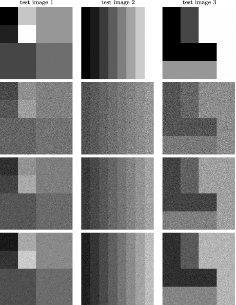
Figure 1: The true test images used in the first numerical experiment (first row), and typical noisy images generated from $\mbox{snr}=1$ (second row), 2 (third row) and 4 (last row). All images are plotted with size $256\times 256$.

For each noisy image, the AIC, BIC and MDL segmentation solutions (6) to (8) were obtained using the merging algorithm in Lee (2000). To verify the result that $\hat{m}\stackrel{{\scriptstyle P}}{{\to}}m^{0}$ (Theorem 3.2), the number of regions in each segmentation solution was counted and the corresponding frequencies are tabulated in Tables 1 to 3. From these tables the following empirical conclusions can be made:

• AIC had a strong tendency to over-estimate $m^{0}$.

• The performance of BIC improved as $n$ increased, and occasionally it over-estimated $m^{0}$.

• For reasonably large snr and $n$, MDL always correctly estimated $m^{0}$.

• For small snr and $n$, MDL under-estimated $m^{0}$. As mentioned before, for such cases some of the region boundaries are hardly visible (see Figure 1).

• When comparing the BIC and MDL results, especially from Table 3, it seems that having the region area and perimeter in the penalty improved the performance.

Table 1: Frequencies of $\hat{m}$ estimated from the noisy images generated from test image 1 for different combinations of snr and $n$. The value of the true $m^{0}$ is 7

		$\bolds{n=64^{2}}$			$\bolds{n=128^{2}}$			$\bolds{n=256^{2}}$			$\bolds{n=512^{2}}$
snr	$\bolds{\hat{m}}$	AIC	BIC	MDL	AIC	BIC	MDL	AIC	BIC	MDL	AIC	BIC	MDL
1	3	$0$	$0$	$0$	$0$	$0$	$0$	$0$	$0$	$0$	$0$	$0$	$0$
	4	$0$	$0$	$0$	$0$	$0$	$0$	$0$	$0$	$0$	$0$	$0$	$0$
	5	$0$	$0$	$101$	$0$	$0$	$0$	$0$	$0$	$0$	$0$	$0$	$0$
	6	$0$	$0$	$237$	$0$	$0$	$0$	$0$	$0$	$0$	$0$	$0$	$0$
	$\mathbf{7}$	$\mathbf{0}$	$\mathbf{485}$	$\mathbf{162}$	$\mathbf{3}$	$\mathbf{495}$	$\mathbf{500}$	$\mathbf{6}$	$\mathbf{499}$	$\mathbf{500}$	$\mathbf{0}$	$\mathbf{500}$	$\mathbf{500}$
	8	$18$	$15$	$0$	$10$	$5$	$0$	$15$	$1$	$0$	$14$	$0$	$0$
	9	$59$	$0$	$0$	$59$	$0$	$0$	$52$	$0$	$0$	$45$	$0$	$0$
	10$+$	$423$	$0$	$0$	$428$	$0$	$0$	$427$	$0$	$0$	$441$	$0$	$0$
2	3	$0$	$0$	$0$	$0$	$0$	$0$	$0$	$0$	$0$	$0$	$0$	$0$
	4	$0$	$0$	$0$	$0$	$0$	$0$	$0$	$0$	$0$	$0$	$0$	$0$
	5	$0$	$0$	$0$	$0$	$0$	$0$	$0$	$0$	$0$	$0$	$0$	$0$
	6	$0$	$0$	$0$	$0$	$0$	$0$	$0$	$0$	$0$	$0$	$0$	$0$
	$\mathbf{7}$	$\mathbf{2}$	$\mathbf{489}$	$\mathbf{500}$	$\mathbf{2}$	$\mathbf{496}$	$\mathbf{500}$	$\mathbf{2}$	$\mathbf{499}$	$\mathbf{500}$	$\mathbf{1}$	$\mathbf{500}$	$\mathbf{500}$
	8	$22$	$11$	$0$	$25$	$4$	$0$	$24$	$1$	$0$	$16$	$0$	$0$
	9	$63$	$0$	$0$	$79$	$0$	$0$	$65$	$0$	$0$	$52$	$0$	$0$
	10$+$	$413$	$0$	$0$	$394$	$0$	$0$	$409$	$0$	$0$	$431$	$0$	$0$
4	3	$0$	$0$	$0$	$0$	$0$	$0$	$0$	$0$	$0$	$0$	$0$	$0$
	4	$0$	$0$	$0$	$0$	$0$	$0$	$0$	$0$	$0$	$0$	$0$	$0$
	5	$0$	$0$	$0$	$0$	$0$	$0$	$0$	$0$	$0$	$0$	$0$	$0$
	6	$0$	$0$	$0$	$0$	$0$	$0$	$0$	$0$	$0$	$0$	$0$	$0$
	$\mathbf{7}$	$\mathbf{3}$	$\mathbf{487}$	$\mathbf{500}$	$\mathbf{0}$	$\mathbf{498}$	$\mathbf{500}$	$\mathbf{3}$	$\mathbf{499}$	$\mathbf{500}$	$\mathbf{0}$	$\mathbf{500}$	$\mathbf{500}$
	8	$19$	$12$	$0$	$17$	$2$	$0$	$9$	$1$	$0$	$1$	$0$	$0$
	9	$64$	$0$	$0$	$54$	$0$	$0$	$31$	$0$	$0$	$10$	$0$	$0$
	10$+$	$414$	$1$	$0$	$429$	$0$	$0$	$457$	$0$	$0$	$489$	$0$	$0$

Table 2: Similar to Table 1 but for test image 2. The value of the true $m^{0}$ is 8

		$\bolds{n=64^{2}}$			$\bolds{n=128^{2}}$			$\bolds{n=256^{2}}$			$\bolds{n=512^{2}}$
snr	$\bolds{\hat{m}}$	AIC	BIC	MDL	AIC	BIC	MDL	AIC	BIC	MDL	AIC	BIC	MDL
1	3	$0$	$0$	$213$	$0$	$0$	$0$	$0$	$0$	$0$	$0$	$0$	$0$
	4	$0$	$0$	$276$	$0$	$0$	$124$	$0$	$0$	$0$	$0$	$0$	$0$
	5	$0$	$1$	$11$	$0$	$0$	$312$	$0$	$0$	$0$	$0$	$0$	$0$
	6	$0$	$23$	$0$	$0$	$0$	$57$	$0$	$0$	$0$	$0$	$0$	$0$
	7	$0$	$127$	$0$	$0$	$0$	$7$	$0$	$0$	$2$	$0$	$0$	$0$
	$\mathbf{8}$	$\mathbf{5}$	$\mathbf{203}$	$\mathbf{0}$	$\mathbf{78}$	$\mathbf{492}$	$\mathbf{0}$	$\mathbf{69}$	$\mathbf{500}$	$\mathbf{498}$	$\mathbf{75}$	$\mathbf{500}$	$\mathbf{500}$
	9	$33$	$114$	$0$	$114$	$6$	$0$	$127$	$0$	$0$	$96$	$0$	$0$
	10$+$	$462$	$32$	$0$	$308$	$2$	$0$	$304$	$0$	$0$	$329$	$0$	$0$
2	3	$0$	$0$	$0$	$0$	$0$	$0$	$0$	$0$	$0$	$0$	$0$	$0$
	4	$0$	$0$	$12$	$0$	$0$	$0$	$0$	$0$	$0$	$0$	$0$	$0$
	5	$0$	$0$	$77$	$0$	$0$	$0$	$0$	$0$	$0$	$0$	$0$	$0$
	6	$0$	$0$	$138$	$0$	$0$	$0$	$0$	$0$	$0$	$0$	$0$	$0$
	7	$0$	$0$	$147$	$0$	$0$	$0$	$0$	$0$	$0$	$0$	$0$	$0$
	$\mathbf{8}$	$\mathbf{85}$	$\mathbf{488}$	$\mathbf{126}$	$\mathbf{82}$	$\mathbf{500}$	$\mathbf{500}$	$\mathbf{92}$	$\mathbf{500}$	$\mathbf{500}$	$\mathbf{66}$	$\mathbf{500}$	$\mathbf{500}$
	9	$119$	$12$	$0$	$114$	$0$	$0$	$95$	$0$	$0$	$94$	$0$	$0$
	10$+$	$296$	$0$	$0$	$304$	$0$	$0$	$313$	$0$	$0$	$340$	$0$	$0$
4	3	$0$	$0$	$0$	$0$	$0$	$0$	$0$	$0$	$0$	$0$	$0$	$0$
	4	$0$	$0$	$0$	$0$	$0$	$0$	$0$	$0$	$0$	$0$	$0$	$0$
	5	$0$	$0$	$0$	$0$	$0$	$0$	$0$	$0$	$0$	$0$	$0$	$0$
	6	$0$	$0$	$0$	$0$	$0$	$0$	$0$	$0$	$0$	$0$	$0$	$0$
	7	$0$	$0$	$0$	$0$	$0$	$0$	$0$	$0$	$0$	$0$	$0$	$0$
	$\mathbf{8}$	$\mathbf{67}$	$\mathbf{499}$	$\mathbf{500}$	$\mathbf{76}$	$\mathbf{500}$	$\mathbf{500}$	$\mathbf{84}$	$\mathbf{500}$	$\mathbf{500}$	$\mathbf{65}$	$\mathbf{500}$	$\mathbf{500}$
	9	$96$	$1$	$0$	$126$	$0$	$0$	$102$	$0$	$0$	$115$	$0$	$0$
	10$+$	$337$	$0$	$0$	$298$	$0$	$0$	$314$	$0$	$0$	$320$	$0$	$0$

Table 3: Similar to Table 1 but for test image 3. The value of the true $m^{0}$ is 4

		$\bolds{n=64^{2}}$			$\bolds{n=128^{2}}$			$\bolds{n=256^{2}}$			$\bolds{n=512^{2}}$
snr	$\bolds{\hat{m}}$	AIC	BIC	MDL	AIC	BIC	MDL	AIC	BIC	MDL	AIC	BIC	MDL
1	3	$0$	$0$	$2$	$0$	$0$	$0$	$0$	$0$	$0$	$0$	$0$	$0$
	$\mathbf{4}$	$\mathbf{9}$	$\mathbf{493}$	$\mathbf{498}$	$\mathbf{4}$	$\mathbf{498}$	$\mathbf{500}$	$\mathbf{6}$	$\mathbf{499}$	$\mathbf{500}$	$\mathbf{8}$	$\mathbf{500}$	$\mathbf{500}$
	5	$34$	$6$	$0$	$33$	$2$	$0$	$35$	$1$	$0$	$22$	$0$	$0$
	6	$63$	$1$	$0$	$60$	$0$	$0$	$70$	$0$	$0$	$57$	$0$	$0$
	7	$94$	$0$	$0$	$97$	$0$	$0$	$86$	$0$	$0$	$98$	$0$	$0$
	8	$80$	$0$	$0$	$113$	$0$	$0$	$103$	$0$	$0$	$95$	$0$	$0$
	9	$99$	$0$	$0$	$96$	$0$	$0$	$87$	$0$	$0$	$88$	$0$	$0$
	10$+$	$121$	$0$	$0$	$97$	$0$	$0$	$113$	$0$	$0$	$132$	$0$	$0$
2	3	$0$	$0$	$0$	$0$	$0$	$0$	$0$	$0$	$0$	$0$	$0$	$0$
	$\mathbf{4}$	$\mathbf{6}$	$\mathbf{494}$	$\mathbf{500}$	$\mathbf{7}$	$\mathbf{498}$	$\mathbf{500}$	$\mathbf{5}$	$\mathbf{499}$	$\mathbf{500}$	$\mathbf{3}$	$\mathbf{500}$	$\mathbf{500}$
	5	$29$	$6$	$0$	$22$	$2$	$0$	$28$	$1$	$0$	$24$	$0$	$0$
	6	$69$	$0$	$0$	$70$	$0$	$0$	$58$	$0$	$0$	$71$	$0$	$0$
	7	$92$	$0$	$0$	$97$	$0$	$0$	$87$	$0$	$0$	$85$	$0$	$0$
	8	$102$	$0$	$0$	$92$	$0$	$0$	$124$	$0$	$0$	$85$	$0$	$0$
	9	$78$	$0$	$0$	$91$	$0$	$0$	$87$	$0$	$0$	$80$	$0$	$0$
	10$+$	$124$	$0$	$0$	$121$	$0$	$0$	$111$	$0$	$0$	$152$	$0$	$0$
4	3	$0$	$0$	$0$	$0$	$0$	$0$	$0$	$0$	$0$	$0$	$0$	$0$
	$\mathbf{4}$	$\mathbf{4}$	$\mathbf{492}$	$\mathbf{500}$	$\mathbf{5}$	$\mathbf{499}$	$\mathbf{500}$	$\mathbf{3}$	$\mathbf{500}$	$\mathbf{500}$	$\mathbf{2}$	$\mathbf{500}$	$\mathbf{500}$
	5	$29$	$8$	$0$	$24$	$1$	$0$	$12$	$0$	$0$	$4$	$0$	$0$
	6	$56$	$0$	$0$	$49$	$0$	$0$	$46$	$0$	$0$	$15$	$0$	$0$
	7	$82$	$0$	$0$	$87$	$0$	$0$	$62$	$0$	$0$	$31$	$0$	$0$
	8	$102$	$0$	$0$	$104$	$0$	$0$	$101$	$0$	$0$	$44$	$0$	$0$
	9	$104$	$0$	$0$	$94$	$0$	$0$	$92$	$0$	$0$	$76$	$0$	$0$
	10$+$	$123$	$0$	$0$	$137$	$0$	$0$	$184$	$0$	$0$	$328$	$0$	$0$

The other major theoretical result that we want to verify is that $\hat{\mathbf{R}}$ converges to $\mathbf{R}^{0}$ (Theorems 3.1 and 3.2). However, it is not as straightforward as verifying $\hat{m}\stackrel{{\scriptstyle P}}{{\to}}m^{0}$, as there is no universally agreed distance metric for measuring the distance between two image partitions $\hat{\mathbf{R}}$ and $\mathbf{R}^{0}$ [although some related work can be found in Baddeley (1992)]. To circumvent this issue, we use a somewhat stricter metric, the mean-squared-error (MSE), defined as $\mbox{MSE}(\hat{f})=\sum_{i=1}^{n}(f_{i}-\hat{f}_{i})^{2}$. The reason we see $\mbox{MSE}(\hat{f})$ as a stricter metric is that, given that $m^{0}$ is correctly estimated, it is extremely likely that $\hat{\mathbf{R}}=\mathbf{R}^{0}$ when $\mbox{MSE}(\hat{f})=0$, but not vice versa.

Table 4: The averaged $\mbox{MSE}(\hat{f})$ values (multiplied by 1,000) for each combination of test image, snr and $n$ for the first simulation experiment. Numbers in parentheses are the ratios $\{\mbox{MSE}(\hat{f})\}^{0.5}/\sigma$. Boldface indicates the smallest value for each experimental setting

Image	snr		$\bolds{n=64^{2}}$	$\bolds{n=128^{2}}$	$\bolds{n=256^{2}}$	$\bolds{n=512^{2}}$
1	1	AIC	$18.58\ (0.09352)$	$4.510\ (0.04607)$	$1.090\ (0.02265)$	$0.2756\ (0.01139)$
		BIC	$\mathbf{6}\bolds{.}\mathbf{193}\ \mbox{{(0.05399)}}$	$0.9575\ (0.02123)$	$0.2244\ (0.01028)$	$\mathbf{0}\bolds{.}\mathbf{05753}\ \mbox{{(0.005203)}}$
		MDL	$31.14\ (0.1211)$	$\mathbf{0}\bolds{.}\mathbf{9304}\ \mbox{{(0.02092)}}$	$\mathbf{0}\bolds{.}\mathbf{2230}\ \mbox{{(0.01024)}}$	$\mathbf{0}\bolds{.}\mathbf{05753}\ \mbox{{(0.005203)}}$
1	2	AIC	$4.196\ (0.08887)$	$1.050\ (0.04447)$	$0.2689\ (0.02250)$	$0.06735\ (0.01126)$
		BIC	$0.9305\ (0.04185)$	$0.2291\ (0.02076)$	$0.05672\ (0.01033)$	$\mathbf{0}\bolds{.}\mathbf{01441}\ \mbox{{(0.005208)}}$
		MDL	$\mathbf{0}\bolds{.}\mathbf{8783}\ \mbox{{(0.04066)}}$	$\mathbf{0}\bolds{.}\mathbf{2236}\ \mbox{{(0.02052)}}$	$\mathbf{0}\bolds{.}\mathbf{05630}\ \mbox{{(0.01029)}}$	$\mathbf{0}\bolds{.}\mathbf{01441}\ \mbox{{(0.005208)}}$
1	4	AIC	$1.076\ (0.09002)$	$0.2736\ (0.04539)$	$0.06671\ (0.02241)$	$0.01682\ (0.01125)$
		BIC	$0.2472\ (0.04314)$	$0.05934\ (0.02114)$	$0.01424\ (0.01035)$	$\mathbf{0}\bolds{.}\mathbf{003550}\ \mbox{{(0.005170)}}$
		MDL	$\mathbf{0}\bolds{.}\mathbf{2280}\ \mbox{{(0.04144)}}$	$\mathbf{0}\bolds{.}\mathbf{05869}\ \mbox{{(0.02102)}}$	$\mathbf{0}\bolds{.}\mathbf{01414}\ \mbox{{(0.01032)}}$	$\mathbf{0}\bolds{.}\mathbf{003550}\ \mbox{{(0.005170)}}$
2	1	AIC	$\mathbf{76}\bolds{.}\mathbf{23}\ \mbox{{(0.1894)}}$	$6.908\ (0.05701)$	$1.661\ (0.02796)$	$0.4176\ (0.01402)$
		BIC	$112.8\ (0.2304)$	$\mathbf{3}\bolds{.}\mathbf{038}\ \mbox{{(0.03781)}}$	$\mathbf{0}\bolds{.}\mathbf{6388}\ \mbox{{(0.01734)}}$	$\mathbf{0}\bolds{.}\mathbf{1617}\ \mbox{{(0.008724)}}$
		MDL	$472.8\ (0.4717)$	$218.2\ (0.3204)$	$0.8846\ (0.02040)$	$\mathbf{0}\bolds{.}\mathbf{1617}\ \mbox{{(0.008724)}}$
2	2	AIC	$6.726\ (0.1125)$	$1.655\ (0.05581)$	$0.4015\ (0.02749)$	$0.1047\ (0.01404)$
		BIC	$\mathbf{3}\bolds{.}\mathbf{212}\ \mbox{{(0.07775)}}$	$\mathbf{0}\bolds{.}\mathbf{6411}\ \mbox{{(0.03474)}}$	$\mathbf{0}\bolds{.}\mathbf{1540}\ \mbox{{(0.01702)}}$	$\mathbf{0}\bolds{.}\mathbf{04023}\ \mbox{{(0.008702)}}$
		MDL	$90.07\ (0.4118)$	$\mathbf{0}\bolds{.}\mathbf{6411}\ \mbox{{(0.03474)}}$	$\mathbf{0}\bolds{.}\mathbf{1540}\ \mbox{{(0.01702)}}$	$\mathbf{0}\bolds{.}\mathbf{04023}\ \mbox{{(0.008702)}}$
2	4	AIC	$1.697\ (0.1130)$	$0.4143\ (0.05585)$	$0.1027\ (0.02780)$	$0.02516\ (0.01376)$
		BIC	$0.6276\ (0.06874)$	$\mathbf{0}\bolds{.}\mathbf{1552}\ \mbox{{(0.03419)}}$	$\mathbf{0}\bolds{.}\mathbf{03902}\ \mbox{{(0.01714)}}$	$\mathbf{0}\bolds{.}\mathbf{01000}\ \mbox{{(0.008678)}}$
		MDL	$\mathbf{0}\bolds{.}\mathbf{6248}\ \mbox{{(0.06859)}}$	$\mathbf{0}\bolds{.}\mathbf{1552}\ \mbox{{(0.03419)}}$	$\mathbf{0}\bolds{.}\mathbf{03902}\ \mbox{{(0.01714)}}$	$\mathbf{0}\bolds{.}\mathbf{01000}\ \mbox{{(0.008678)}}$
3	1	AIC	$11.88\ (0.07476)$	$2.870\ (0.03675)$	$0.7030\ (0.01819)$	$0.1759\ (0.009098)$
		BIC	$\mathbf{2}\bolds{.}\mathbf{078}\ \mbox{{(0.03127)}}$	$0.4024\ (0.01376)$	$0.09679\ (0.006749)$	$\mathbf{0}\bolds{.}\mathbf{02367}\ \mbox{{(0.003338)}}$
		MDL	$2.545\ (0.03461)$	$\mathbf{0}\bolds{.}\mathbf{3927}\ \mbox{{(0.01359)}}$	$\mathbf{0}\bolds{.}\mathbf{09558}\ \mbox{{(0.006707)}}$	$\mathbf{0}\bolds{.}\mathbf{02367}\ \mbox{{(0.003338)}}$
3	2	AIC	$2.932\ (0.07429)$	$0.7225\ (0.03688)$	$0.1822\ (0.01852)$	$0.04568\ (0.009272)$
		BIC	$0.4140\ (0.02792)$	$0.1053\ (0.01408)$	$0.02521\ (0.006889)$	$\mathbf{0}\bolds{.}\mathbf{006404}\ \mbox{{(0.003472)}}$
		MDL	$\mathbf{0}\bolds{.}\mathbf{3915}\ \mbox{{(0.02715)}}$	$\mathbf{0}\bolds{.}\mathbf{1028}\ \mbox{{(0.01391)}}$	$\mathbf{0}\bolds{.}\mathbf{02494}\ \mbox{{(0.006852)}}$	$\mathbf{0}\bolds{.}\mathbf{006404}\ \mbox{{(0.003472)}}$
3	4	AIC	$0.7430\ (0.07479)$	$0.1839\ (0.03721)$	$0.04468\ (0.01834)$	$0.01101\ (0.009106)$
		BIC	$0.1106\ (0.02885)$	$0.02441\ (0.01356)$	$\mathbf{0}\bolds{.}\mathbf{005919}\ \mbox{{(0.006676)}}$	$\mathbf{0}\bolds{.}\mathbf{001478}\ \mbox{{(0.003336)}}$
		MDL	$\mathbf{0}\bolds{.}\mathbf{1041}\ \mbox{{(0.02799)}}$	$\mathbf{0}\bolds{.}\mathbf{02415}\ \mbox{{(0.01348)}}$	$\mathbf{0}\bolds{.}\mathbf{005919}\ \mbox{{(0.006676)}}$	$\mathbf{0}\bolds{.}\mathbf{001478}\ \mbox{{(0.003336)}}$

The averaged values of $\mbox{MSE}(\hat{f})$ and $\{\mbox{MSE}(\hat{f})\}^{0.5}/\sigma$ are listed in Table 4.1, where $\sigma^{2}$ is the true noise variance. As expected, the larger the image size $n$, the smaller these values are. Also, the corresponding figures from BIC and MDL are substantially smaller than those from AIC for large $n$. For small $n$ and snr, MDL produced poor $\mbox{MSE}(\hat{f})$ values. It is due to the fact that MDL under-estimates $m^{0}$.

4.2 Experiment 2

Altogether six test images were used in this second numerical experiment. When comparing to the three test images used in the first experiments, the shapes of the objects in these six images are more complicated; see Figure 2.

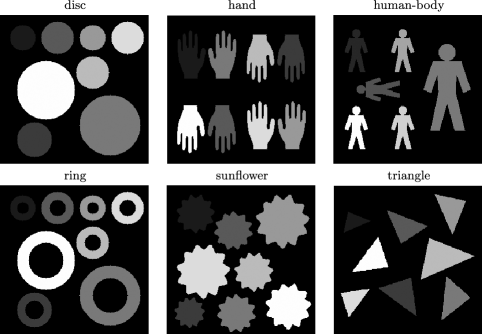
Figure 2: The true test images used in the second numerical experiment.

We repeated the same testing procedure as above, but only for $n=256^{2}$. For each test image, the averages of the estimated number of regions for AIC, BIC and MDL segmentation solutions are tabulated in Table 4.2. The standard errors of these averages are also reported. We have also computed the averaged values of of $\mbox{MSE}(\hat{f})$ and $\{\mbox{MSE}(\hat{f})\}^{0.5}/\sigma$; they are listed in Table 4.2. Empirical conclusions

Table 5: The averaged $\hat{m}$ values for the second numerical experiment. Numbers in parentheses are estimated standard errors. The true values of $m$ (i.e., $m^{0}$) are listed in square brackets

Image $\bolds{[m^{0}]}$		$\bolds{\mathrm{snr}=1}$	$\bolds{\mathrm{snr}=2}$	$\bolds{\mathrm{snr}=4}$
Disc [8]	AIC	$83.2\ (0.274)$	$69.0\ (0.268)$	$48.2\ (0.243)$
	BIC	$20.9\ (0.165)$	$16.5\ (0.123)$	$9.94\ (0.0689)$
	MDL	$6.38\ (0.0219)$	$7.06\ (0.0107)$	$8.05\ (0.014)$
Hand [8]	AIC	$77.8\ (0.259)$	$63.7\ (0.247)$	$39.6\ (0.219)$
	BIC	$20.4\ (0.139)$	$15.5\ (0.106)$	$9.45\ (0.0636)$
	MDL	$6.84\ (0.0259)$	$8.05\ (0.0245)$	$8.13\ (0.0168)$
Human-body [6]	AIC	$67.7\ (0.268)$	$47.9\ (0.247)$	$25.3\ (0.187)$
	BIC	$15.7\ (0.130)$	$8.97\ (0.0951)$	$6.15\ (0.0194)$
	MDL	$5.04\ (0.00964)$	$6.23\ (0.0253)$	$6.03\ (0.00739)$
Ring [16]	AIC	$81.1\ (0.266)$	$69.6\ (0.244)$	$48.9\ (0.218)$
	BIC	$24.8\ (0.153)$	$22.1\ (0.120)$	$16.7\ (0.0613)$
	MDL	$11.2\ (0.0279)$	$13.9\ (0.0184)$	$15.2\ (0.0189)$
Sunflower [8]	AIC	$81.8\ (0.289)$	$67.6\ (0.250)$	$47.8\ (0.259)$
	BIC	$20.0\ (0.153)$	$15.7\ (0.123)$	$10.2\ (0.0939)$
	MDL	$6.07\ (0.0117)$	$7.41\ (0.0222)$	$8.15\ (0.0224)$
Triangle [8]	AIC	$75.7\ (0.276)$	$62.6\ (0.248)$	$35.4\ (0.220)$
	BIC	$18.6\ (0.138)$	$14.5\ (0.119)$	$8.48\ (0.0313)$
	MDL	$6.97\ (0.0101)$	$7.57\ (0.0223)$	$7.99\ (0.00597)$

obtainable from these two tables are similar to those from the first experiment. A noteworthy observation is that, when snr is not large, the tendency for BIC to over-estimate $m^{0}$ is more apparent for these new test images, that is, when the object boundaries are more complex.

Table 6: The averaged $\mbox{MSE}(\hat{f})$ values (multiplied by 1,000) for each combination of test image and snr. Numbers in parentheses are the ratios $\{\mbox{MSE}(\hat{f})\}^{0.5}/\sigma$. Boldface indicates the smallest value for each experimental setting

Image		$\bolds{\mathrm{snr}=1}$	$\bolds{\mathrm{snr}=2}$	$\bolds{\mathrm{snr}=4}$
Disc	AIC	475.4 (0.2333)	81.55 (0.1932)	$10.44\ (0.1383)$
	BIC	405.7 (0.2155)	65.78 (0.1735)	$7.811\ (0.1196)$
	MDL	428.7 (0.2215)	69.56 (0.1784)	$\mathbf{7}\mbox{{.763}}\ \mbox{{(0.1192)}}$
Hand	AIC	504.9 (0.2950)	79.51 (0.2342)	$10.75\ (0.1722)$
	BIC	465.3 (0.2832)	70.62 (0.2207)	$\mathbf{9}\mbox{{.522}}\ \mbox{{(0.1621)}}$
	MDL	485.4 (0.2893)	71.22 (0.2216)	$9.853\ (0.1649)$
Human-body	AIC	135.3 (0.2443)	19.82 (0.1870)	$1.491\ (0.1026)$
	BIC	119.9 (0.2300)	17.17 (0.1741)	$\mathbf{1}\mbox{{.208}}\ \mbox{{(0.09234)}}$
	MDL	120.9 (0.2309)	17.53 (0.1759)	$1.217\ (0.09269)$
Ring	AIC	541.1 (0.2774)	81.89 (0.2158)	$11.00\ (0.1582)$
	BIC	493.2 (0.2648)	70.89 (0.2008)	$\mathbf{9}\mbox{{.314}}\ \mbox{{(0.1456)}}$
	MDL	520.8 (0.2721)	73.74 (0.2048)	$9.572\ (0.1476)$
Sunflower	AIC	527.3 (0.2517)	89.43 (0.2073)	$12.98\ (0.1580)$
	BIC	464.1 (0.2362)	74.97 (0.1898)	$\mathbf{10}\mbox{{.54}}\ \mbox{{(0.1423)}}$
	MDL	488.3 (0.2422)	83.32 (0.2001)	$10.74\ (0.1437)$
Triangle	AIC	219.8 (0.2165)	32.64 (0.1668)	$3.242\ (0.1051)$
	BIC	182.6 (0.1973)	24.84 (0.1455)	$\mathbf{2}\mbox{{.326}}\ \mbox{{(0.08906)}}$
	MDL	168.9 (0.1897)	23.50 (0.1416)	$2.353\ (0.08957)$

5 Real image segmentation

Figure 3(a) displays a synthetic aperture radar (SAR) image of a rural area. It is of dimension $250\times 250$ and is made available by Dr. E. Attema of the European Space Research and Technology Centre. The image has been log-transformed in order to stabilize the noise variance. It would be useful to segment the image into regions of similar vegetation.

Notice that the image is extremely noisy (i.e., low snr) and hence difficult to obtain a good segmentation. Therefore, we applied the MDL criterion to segment the image, as the simulation results above suggest that both AIC and BIC would heavily oversegment the image. The MDL segmented result, which consists of 34 segmented regions, is given in Figure 3(b).

Even though a Gaussian noise assumption may not be appropriate for this SAR image, the MDL criterion produced a reasonable segmentation. The most apparent weakness of the segmentation is the roughness of the boundaries (many of which should clearly be straight) and the failure to detect some narrow regions. This weakness can be (at least partially) attributed to the noisy nature of the image.

6 Concluding remarks

This paper fills an important gap in the image segmentation literature by providing a systematic investigation into the theoretical properties of some popular information theoretic segmentation methods. It is shown that both the BIC and the MDL segmentation solutions are statistically consistent for recovering the number of objects together with their boundaries in an image. These theoretical results are empirically verified by simulation experiments. We also note that our theoretical results can be straightforwardly extended to higher-dimensional problems, such as volumetric or movie segmentation.

The numerical results from the simulation experiments also revealed some discrepancy in the finite sample performances between BIC and MDL, which can be attributed to the fact that the region area and perimeter enter explicitly into the MDL segmentation criterion but not BIC. These results seem to suggest that, when both the number of pixels $n$ and the signal-to-noise ratio (snr) are not small, MDL is capable of producing very stable and reliable results. For those cases when both $n$ and snr are small, MDL always under-estimated the number of regions, which led to poor MSE values. However, when one inspects the noisy images that correspond to such cases, one can see that, due to the high noise variance, some of the adjacent regions are hardly distinguishable, which explains the under-estimation of MDL. Overall the numerical results also suggest that BIC has a tendency to over-estimate the number of regions, and for those high noise variance cases, this tendency actually worked in favor of the situation. Considering all these factors, in practice if the image to be segmented is not too noisy or not too small in size, one may consider using MDL, otherwise, use BIC.

Appendix: Proofs

This Appendix first provides the proofs for Theorems 3.1 and 3.2 in Appendices .1 and .2. Appendix .3 covers the BIC and AIC procedures.

.1 Proof of Theorem 3.1

We first provide a number of auxiliary results and will throughout use the following conventions. The true segmentation of $[0,1]^{2}$ will be denoted by $R_{1}^{0},\ldots,R_{m^{0}}^{0}$. All other segmentations will be denoted $R_{1},\ldots,R_{m}$, while the MDL-based estimates will be $\hat{R}_{1},\ldots,\hat{R}_{m}$. Recall that in the situation of Theorem 3.1, the number of segments, $m=m^{0}$, is assumed known.

Lemma .1

Let $y_{i}=f(\mbox{$x$}_{i})+\varepsilon_{i}$, $i=1,\ldots,n$, be random variables with $f(\mbox{$x$})=\mu$ for all $\mbox{$x$}\in[0,1]^{2}$ and design points $\Xi_{n}=\{\mbox{$x$}_{1},\ldots,\mbox{$x$}_{n}\}\subset[0,1]^{2}$ satisfying (9). Assume furthermore that $\{\varepsilon_{i}\}$ is a sequence of independent, identically distributed random variables with zero mean and variance $\sigma^{2}$. Fix a subset $R\subset[0,1]^{2}$, and let $a=\#\mathcal{A}$ for $\mathcal{A}=\{i\colon\mbox{$x$}_{i}\in\Xi_{n}\cap R\}$. Define the estimators

$$\hat{\mu}(R)=\frac{1}{a}\sum_{i\in\mathcal{A}}y_{i}\quad\mbox{and}\quad\hat{\sigma}^{2}(R)=\frac{1}{a}\sum_{i\in\mathcal{A}}\{y_{i}-\hat{\mu}(R)\}^{2}.\vspace*{-2pt}$$

Then $\hat{\mu}(R)\to\mu$ and $\hat{\sigma}^{2}(R)\to\sigma^{2}$ with probability one as $n\to\infty$.

Notice that the sequence $\{y_{i}\}$ is globally independent and identically distributed with mean $\mu$ and variance $\sigma^{2}$, so in particular on any subset $R\subset[0,1]^{2}$. Both assertions of the lemma follow therefore directly from the strong law of large numbers after recognizing that $a\to\infty$ as $n\to\infty$ because of (9).

Lemma .2

Let $\{y_{i}\}$ be the sequence of random variables defined in (3). Fix a subset $R\subset[0,1]^{2}$ and denote by $\hat{\mu}(R)$ the sample mean defined in Lemma .1. Then, $\hat{\mu}(R)\to\mu_{*}$ with probability one, where the limit $\mu_{*}(R)$ is defined in (.1) below.

Utilizing the true segmentation, we can write

$$R=\bigcup_{\nu=1}^{m}R\cap R_{\nu}^{0}=\bigcup_{\ell=1}^{2}\bigcup_{\nu\in\mathcal{I}_{\ell}}R\cap R_{\nu}^{0},$$

where $\mathcal{I}_{1}=\{\nu\colon R_{\nu}^{0}\subset R\}$ and $\mathcal{I}_{2}=\{\nu\colon R\cap R_{\nu}^{0}\not=\varnothing\}\setminus\mathcal{I}_{1}$, thus ignoring those $\nu$ for which $R\cap R_{\nu}^{0}=\varnothing$ on the right-hand side of the last display. Define $\tilde{a}_{\nu}^{0}=\#\tilde{\mathcal{A}}_{\nu}^{0}$ for $\tilde{\mathcal{A}}_{\nu}^{0}=\{i\colon\mbox{$x$}_{i}\in\Xi_{n}\cap R\cap R_{\nu}^{0}\}$ and $a_{\nu}^{0}=\#\mathcal{A}_{\nu}^{0}$ for $\mathcal{A}_{\nu}^{0}=\{i\colon\mbox{$x$}_{i}\in\Xi_{n}\cap R_{\nu}^{0}\}$. It follows from an application of Lemma .1 that

$$\hat{\mu}(R)=\frac{1}{a}\sum_{i\in A}y_{i} = \frac{1}{a}\biggl{(}\sum_{\nu\in\mathcal{I}_{1}}\sum_{i\in\mathcal{A}_{\nu}^{0}}y_{i}+\sum_{\nu\in\mathcal{I}_{2}}\sum_{i\in\tilde{\mathcal{A}}_{\nu}^{0}}y_{i}\biggr{)}$$

$$= \frac{1}{a}\biggl{(}\sum_{\nu\in\mathcal{I}_{1}}a_{\nu}^{0}\mu_{\nu}^{0}+\sum_{\nu\in\mathcal{I}_{2}}\tilde{a}_{\nu}^{0}\mu_{\nu}^{0}\biggr{)}$$

$$\to \frac{1}{\alpha}\biggl{(}\sum_{\nu\in\mathcal{I}_{1}}\alpha_{\nu}^{0}\mu_{\nu}^{0}+\sum_{\nu\in\mathcal{I}_{2}}\tilde{\alpha}_{\nu}^{0}\mu_{\nu}^{0}\biggr{)}=:\mu_{*}(R)$$

with probability one as $n\to\infty$, on account of (9) and by assumption on the representation of the number of design points in any given region ($a=\lfloor\alpha n\rfloor$, $a_{\nu}^{0}=\lfloor\alpha_{\nu}^{0}n\rfloor$ and $\tilde{a}_{\nu}^{0}=\lfloor\tilde{\alpha}_{\nu}^{0}n\rfloor$).

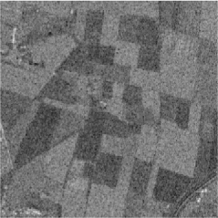
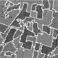
(a)	(b)

Figure 3: Real image segmentation. (a): Observed SAR image and (b): MDL segmented result.

Lemma .3

Let $\{y_{i}\}$ be the sequence of random variables defined in (3). Fix a subset $R\subset[0,1]^{2}$ and denote by $\hat{\sigma}^{2}(R)$ the variance estimator defined in Lemma .1. Then, $\hat{\sigma}^{2}(R)\to\sigma^{2}+\sigma^{2}_{*}(R)$ with probability one, where $\sigma^{2}_{*}(R)$ is defined in (.1) below.

Using the notation of the proof of Lemma .2 and applying similar arguments yields the decomposition

$$\hat{\sigma}^{2}(R)=\frac{1}{a}\sum_{i\in\mathcal{A}}\{y_{i}-\hat{\mu}(R)\}^{2}=\frac{1}{a}\sum_{\nu\in\mathcal{I}_{1}}\sum_{i\in\mathcal{A}_{\nu}^{0}}\{y_{i}-\hat{\mu}(R)\}^{2}+\frac{1}{a}\sum_{\nu\in\mathcal{I}_{1}}\sum_{i\in\tilde{\mathcal{A}}_{\nu}^{0}}\{y_{i}-\hat{\mu}(R)\}^{2}.$$

Let first $\nu\in\mathcal{I}_{1}$. By definition of $\mathcal{I}_{1}$, $R_{\nu}^{0}$ is completely contained in $R$. Therefore, adding and subtracting the true value $\mu_{\nu}^{0}$ from each of the terms $y_{i}-\hat{\mu}(R)$ and subsequently solving the square leads to

$$\frac{1}{a}\sum_{i\in\mathcal{A}_{\nu}^{0}}\{y_{i}-\hat{\mu}(R)\}^{2} = \frac{1}{a}\sum_{i\in\mathcal{A}_{\nu}^{0}}(y_{i}-\mu_{\nu}^{0})^{2}-\frac{2}{a}\sum_{i\in\mathcal{A}_{\nu}^{0}}(y_{i}-\mu_{\nu}^{0})\{\mu_{\nu}^{0}-\hat{\mu}(R)\}$$

$${}+\frac{1}{a}\sum_{i\in\mathcal{A}_{\nu}^{0}}\{\mu_{\nu}^{0}-\hat{\mu}(R)\}^{2}$$

$$= S_{1}+S_{2}+S_{3}.$$

Lemma .1 implies for the first term that

$$S_{1}=\frac{a_{\nu}^{0}}{a}\frac{1}{a_{\nu}^{0}}\sum_{i\in\mathcal{A}_{\nu}^{0}}(y_{i}-\mu_{\nu}^{0})^{2}\to\frac{\alpha_{\nu}^{0}}{\alpha}\sigma^{2}\qquad\mbox{a.s.}\qquad(n\to\infty).$$

The second term $S_{2}$ is asymptotically small with probability one. To see this, observe that, by Lemma .2, $\mu_{\nu}^{0}-\hat{\mu}(R)$ converges a.s. to $M_{\nu}^{0}=\mu_{\nu}^{0}-\mu_{*}(R)$ as $n\to\infty$. For two sequences $\{\xi_{n}\}$ and $\{\zeta_{n}\}$ of real numbers, write $\xi_{n}\sim\zeta_{n}$ if $\lim_{n}\xi_{n}\zeta_{n}^{-1}=1$. Then, using the strong law of large numbers for the i.i.d. sequence $\{\varepsilon_{i}\}$, we obtain that

$$S_{2}\sim\frac{2M_{\nu}^{0}}{a}\sum_{i\in\mathcal{A}_{\nu}^{0}}(y_{i}-\mu_{\nu}^{0})=\frac{2M_{\nu}^{0}}{a}\sum_{i\in\mathcal{A}_{\nu}^{0}}\varepsilon_{i}\to 0\qquad\mbox{a.s.}\qquad(n\to\infty).$$

Finally, by Lemma .2,

$$S_{3}=\frac{a_{\nu}^{0}}{a}\{\mu_{\nu}^{0}-\hat{\mu}(R)\}^{2}\to\frac{\alpha_{\nu}^{0}}{\alpha}\{\mu_{\nu}^{0}-\mu_{*}(R)\}^{2}\qquad\mbox{a.s.}\qquad(n\to\infty).$$

Let now $\nu\in\mathcal{I}_{2}$. Then the region $R_{\nu}^{0}$ of the true segmentation is only partially contained in $R$. This means that, while all computations can be performed along the blueprint for the case $\nu\in\mathcal{I}_{1}$, $\tilde{a}_{\nu}^{0}$, $\alpha_{\nu}^{0}$ and $\tilde{\mathcal{A}}_{\nu}^{0}$ have to be used in place of their respective counterparts $a_{\nu}^{0}$, $\alpha_{\nu}^{0}$ and $\mathcal{A}_{\nu}^{0}$. Combining these results, we arrive at the almost sure convergence

$$\hat{\sigma}^{2}(R) \to \frac{\sigma^{2}}{\alpha}\biggl{(}\sum_{\nu\in\mathcal{I}_{1}}\alpha_{\nu}^{0}+\sum_{\nu\in\mathcal{I}_{2}}\tilde{\alpha}_{\nu}^{0}\biggr{)}$$

$${}+\frac{1}{\alpha}\biggl{[}\sum_{\nu\in\mathcal{I}_{1}}\alpha_{\nu}^{0}\{\mu_{\nu}^{0}-\mu_{*}(R)\}^{2}+\sum_{\nu\in\mathcal{I}_{2}}\tilde{\alpha}_{\nu}^{0}\{\mu_{\nu}^{0}-\mu_{*}(R)\}^{2}\biggr{]}$$

$$= \sigma^{2}+\sigma_{*}^{2}(R)$$

since $\sum_{\mathcal{I}_{1}}\alpha_{\nu}^{0}+\sum_{\mathcal{I}_{2}}\tilde{\alpha}_{\nu}^{0}=\alpha$. This proves the assertion.

Lemma .4

Let $\{y_{i}\}$ be the sequence of random variables defined in (3). Let $\epsilon>0$ such that, for appropriately chosen $\mathbf{z}_{\nu}\in R_{\nu}$ in a segmentation $\mathbf{R}=(R_{1},\ldots,R_{m})$,

$$B_{\epsilon}(\mathbf{z}_{\nu})\subset R_{\nu}\qquad\mbox{for all }\nu=1,\ldots,m=m^{0}.$$ (12)

Let $\mathcal{R}_{\epsilon}=\{\mathbf{R}\colon\bigcup_{\nu}R_{\nu}\mbox{ satisfying (\ref{criterion}) such that }a_{\nu}=\lfloor n\alpha_{\nu}\rfloor,\sum_{\nu}\alpha_{\nu}=1\}$. Then

$$\hat{\mathbf{R}}=\mathop{\arg\min}_{\mathbf{R}\in\mathcal{R}_{\epsilon}}\frac{2}{n}{\mathrm{MDL}}(m^{0},\mathbf{R})\to\mathbf{R}^{0}\qquad\mbox{a.s.}\qquad(n\to\infty),$$

where $\mathbf{R}^{0}$ denotes the true segmentation of $[0,1]^{2}$.

Assume that the MDL estimator is not strongly consistent. Thus $\hat{\mathbf{R}}$ does not converge with probability one to $\mathbf{R}^{0}$ as $n\to\infty$. By boundedness, there exists a monotonically increasing subsequence $\{n_{j}\}$ along which $\hat{\mathbf{R}}_{n_{j}}\to\mathbf{R}^{*}$ with probability one, with the limit $\mathbf{R}^{*}$ being a member of $\mathcal{R}_{\epsilon}$, and $\lambda^{2}(\mathbf{R}^{*}\Delta\mathbf{R}^{0})>0$ with probability one. Note that we must have also that $\hat{\alpha}_{\nu}\to\hat{\alpha}_{\nu}^{*}$ along the same subsequence. Note that, with probability one, $\frac{2}{n}{\mathrm{MDL}}(m^{0},\mathbf{R})\sim\log(\frac{1}{n}\mathrm{RSS}_{m^{0}})$, where $\sim$ is defined in the proof of Lemma .3, and that, for $\mathbf{R}=\mathbf{R}^{*}$,

$$\frac{1}{n}\mathrm{RSS}_{m^{0}}=\frac{1}{n}\sum_{\nu=1}^{m^{0}}\sum_{i\in\mathcal{A}_{\nu}^{*}}\{y_{i}-\hat{\mu}(R_{\nu}^{*})\}^{2}$$

adopting notation from before. For any $\nu$, there are now two options: either $R_{\nu}^{*}$ is contained in a region of the true segmentation, or $R_{\nu}^{*}$ has nontrivial intersections with more than one region of the true segmentation. In the first case, $R_{\nu}^{*}\subset R_{\kappa}^{0}$ for some $\kappa$. Hence, Lemma .1 implies that

$$\frac{1}{n}\sum_{i\in\mathcal{A}_{\nu}^{*}}\{y_{i}-\hat{\mu}(R_{\nu}^{*})\}^{2}\to\alpha_{\nu}^{*}\sigma^{2}\qquad\mbox{a.s.}\qquad(n\to\infty).$$

In the second case, $R_{\nu}^{*}=\bigcup_{\kappa}R_{\nu}^{*}\cap R_{\kappa}^{0}$, where the disjoint union contains at least two elements. Then, Lemma .3 yields that

$$\frac{1}{n}\sum_{i\in\mathcal{A}_{\nu}^{*}}\{y_{i}-\hat{\mu}(R_{\nu}^{*})\}^{2}\to\alpha_{\nu}^{*}\sigma^{2}+\sigma^{2}_{*}\qquad\mbox{a.s.}\qquad(n\to\infty),$$

where $\sigma_{*}^{2}=\sum_{\nu}\alpha_{\nu}^{*}\sigma^{2}_{*}(R_{\nu}^{*})$ with $\sigma^{*}(R_{\nu}^{*})$ as in Lemma .3. Observe that, on account of $\mathbf{R}^{*}\not=\mathbf{R}^{0}$ [in the sense that $\lambda^{2}(\mathbf{R}^{*}\Delta\mathbf{R}^{0})\not=0$ almost surely], we have $\sigma_{*}^{2}>0$. On the other hand, $\sigma_{*}^{2}=0$ if the true segmentation $\mathbf{R}^{0}$ were used. Consequently, exploiting the continuity and strict concavity of the logarithm, we arrive at

$$\lim_{n\to\infty}\frac{2}{n}{\mathrm{MDL}}(m^{0},\mathbf{R}^{*}) > \sum_{\nu=1}^{m^{0}}\alpha_{\nu}^{0}\log\sigma^{2}=\log\sigma^{2}=\lim_{n\to\infty}\frac{2}{n}{\mathrm{MDL}}(m^{0},\mathbf{R}^{0})$$

$$\geq \lim_{n\to\infty}\frac{2}{n}{\mathrm{MDL}}(m^{0},\mathbf{R}^{*}),$$

which is a contradiction. Hence, $\hat{\mathbf{R}}$ is strongly consistent for $\mathbf{R}^{0}$.

.2 Proof of Theorem 3.2

Lemma .5

Let $\{y_{i}\}$ be the sequence of random variables defined in (3). If

$$(\hat{m},\hat{\mathbf{R}})=\mathop{\arg\min}_{m\leq M\mathbf{R}\in\mathcal{R}_{\epsilon}}\frac{2}{n}{\mathrm{MDL}}(m,\mathbf{R}),$$

then $P(\hat{m}\geq m^{0})\to 1$ as $n\to\infty$.

Notice that it follows from the proof of Lemma .4 that$\frac{1}{n}\mathrm{RSS}_{m^{0}}\to\sigma^{2}$ with probability one, provided the true segmentation $\mathbf{R}^{0}$ is used in the computations. If $\hat{m}<m^{0}$, then there is at least one $\hat{R}_{\nu}$ containing two or more true regions $R_{\kappa}^{0}$. It follows as in the proofs of Lemmas .3 and .4 that $P(\frac{1}{n}\mathrm{RSS}_{m}>\sigma^{2}+\epsilon)\to 1$ as $n\to\infty$ for a suitably chosen $\epsilon>0$. This implies the claim.

Lemma .6

Let $\{y_{i}\}$ be the sequence of random variables defined in (3). If $m^{0}<m\leq M$, then, for all $\nu=1,\ldots,m^{0}$,

$$P\{\hat{\mathbf{R}}\in C_{\nu}^{0}(n)\}\to 0\qquad(n\to\infty),$$

where $C_{\nu}^{0}(n)=\{\mathbf{R}=(R_{1},\ldots,R_{m})\colon\partial R_{\kappa}\notin\partial R_{\nu}^{0}+B_{\ell(n)}(0),\kappa=1,\ldots,m\}$.

Fix $1\leq\nu\leq m^{0}$, and let $\mathbf{R}\in C^{0}_{\nu}(n)$. Because of the continuity of $\partial R_{\nu}^{0}$, there is a $\mathbf{z}_{\nu}\in\partial R_{\nu}^{0}$ such that $\partial R_{\kappa}\cap B_{\ell(n)}(\mathbf{z}_{\nu})=\varnothing$ for all $\kappa=1,\ldots,m$. Define $\tilde{\mathbf{R}}$ as the segmentation that includes all regions of the form

$$R_{\kappa}\cap R_{\nu^{\prime}}^{0}\cap B^{c}_{\ell(n)}(\mathbf{z}_{\nu}),\qquad\kappa=1,\ldots,m;\nu^{\prime}=1,\ldots,m^{0},$$

and $B_{\ell(n)}(\mathbf{z}_{\nu})$. Clearly, $\mathrm{RSS}(\mathbf{R})\geq\mathrm{RSS}(\tilde{\mathbf{R}})$, where we use the notations$\mathrm{RSS}(\mathbf{R})$ and $\mathrm{RSS}(\tilde{\mathbf{R}})$ for the residual sums of squares based on the respective segmentations $\mathbf{R}$ and $\tilde{\mathbf{R}}$. Decomposing according to the true segmentation $\mathbf{R}^{0}$ leads to comparisons of the following types. Consider first the case $R_{\nu^{\prime}}^{0}\cap B_{\ell(n)}(\mathbf{z}_{\nu})=\varnothing$. Then, it follows as in Lemma 4 of Yao (1988) that

$$0\leq\sum_{i\in\mathcal{A}_{\nu^{\prime}}^{0}}\varepsilon_{i}^{2}-\sum_{\kappa\in\mathcal{I}_{\nu^{\prime}}}\sum_{i\in\tilde{\mathcal{A}}_{\kappa}}\{y_{i}-\hat{\mu}(\tilde{R}_{\kappa})\}^{2}=\mathcal{O}_{P}(\ln n)\qquad(n\to\infty),$$

where $\mathcal{I}_{\nu^{\prime}}=\{\kappa\colon\tilde{R}_{\kappa}\subset R_{\nu^{\prime}}^{0}\}$, $\mathcal{A}_{\nu^{\prime}}^{0}=\{i\colon\mbox{$x$}_{i}\in\Xi_{n}\cap R_{\nu^{\prime}}^{0}\}$ and $\tilde{\mathcal{A}}_{\kappa}=\{i\colon\mbox{$x$}_{i}\in\Xi_{n}\cap\tilde{R}_{\kappa}\}$. The rate on the right-hand side of the last display explicitly uses that the noise $\{\varepsilon_{i}\}$ follows a normal law and does not need to be true for arbitrary noise distributions [compare the remark on page 188 of Yao (1988)]. Consider next the case $R_{\nu^{\prime}}^{0}\cap B_{\ell(n)}(\mathbf{z}_{\nu})\not=\varnothing$. Observe that the number of design points in $B_{\ell(n)}(\mathbf{z}_{\nu})$ is proportional to $\ln^{2}n$, while the number of design points in any $\tilde{R}_{\nu}$ is proportional to the sample size $n$. Any region $\tilde{R}_{\nu}\in\tilde{\mathbf{R}}$ obtained from a nontrivial intersection with $B_{\ell(n)}^{c}(\mathbf{z}_{\nu})$ has therefore the number of elements reduced by a factor proportional to $\ln^{2}n$. This, however, is negligible compared to $n$ in the long run. Therefore, the same arguments as before imply also that

$$0\leq\sum_{i\in\mathcal{C}^{0}_{\nu^{\prime}}}\varepsilon_{i}^{2}-\sum_{\kappa\in\mathcal{J}_{\nu^{\prime}}}\sum_{i\in\tilde{\mathcal{A}}_{\kappa}}\{y_{i}-\hat{\mu}(\tilde{R}_{\kappa})\}^{2}=\mathcal{O}_{P}(\ln n)\qquad(n\to\infty),$$

where $\mathcal{C}_{\nu^{\prime}}^{0}=\mathcal{A}_{\nu^{\prime}}^{0}\setminus\mathcal{B}_{\nu^{\prime}}$ with $\mathcal{B}_{\nu^{\prime}}=\{i\colon\mbox{$x$}_{i}\in\Xi_{n}\cap B_{\ell(n)}(\mathbf{z}_{\nu})\cap R_{\nu^{\prime}}^{0}\}$, and $\mathcal{J}_{\nu^{\prime}}=\{\kappa\colon\tilde{R}_{\kappa}\subset R_{\nu^{\prime}}^{0}\cap B_{\ell(n)}^{c}(\mathbf{z}_{\nu})\}$. It remains to investigate the region $B_{\ell(n)}(\mathbf{z}_{\nu})$ itself. Without loss of generality assume that $B_{\ell(n)}(\mathbf{z}_{\nu})$ intersects, apart from $R_{\nu}^{0}$, only one more true regions $R_{\nu^{\prime}}^{0}$ as the general case can be handled in a similar fashion. Notice that $b=\#\{B_{\ell(n)}(\mathbf{z}_{\nu})\cap\Xi_{n}\}=\lfloor\beta n\rfloor\sim\ln^{2}n$ by definition. Let furthermore $b_{\nu}=\#\{\Xi_{n}\cap R_{\nu}^{0}\cap B_{\ell(n)}(\mathbf{z}_{\nu})\}$ and $b_{\nu^{\prime}}=\#\{\Xi_{n}\cap R_{\nu^{\prime}}^{0}\cap B_{\ell(n)}(\mathbf{z}_{\nu})\}$. Then, we must have $b_{\nu}=\lfloor\beta_{\nu}n\rfloor\sim\ln^{2}n$ and $b_{\nu^{\prime}}=\lfloor\beta_{\nu^{\prime}}n\rfloor\sim\ln^{2}n$ for appropriate $\beta_{\nu}$ and $\beta_{\nu^{\prime}}$ satisfying $\beta_{\nu}+\beta_{\nu^{\prime}}=\beta$. Now, utilizing that $y_{i}-\hat{\mu}(B_{\ell(n)}(\mathbf{z}_{\nu}))=\varepsilon_{i}+\mu_{\nu}-\hat{\mu}(B_{\ell(n)}(\mathbf{z}_{\nu}))$ on $R_{\nu}^{0}$ and $y_{i}-\hat{\mu}(B_{\ell(n)}(\mathbf{z}_{\nu}))=\varepsilon_{i}+\mu_{\nu^{\prime}}-\hat{\mu}(B_{\ell(n)}(\mathbf{z}_{\nu}))$ on $R_{\nu^{\prime}}^{0}$, we obtain that

$$\frac{1}{b}\biggl{[}\sum_{i\in\mathcal{B}_{\nu}^{*}}\epsilon_{i}^{2}-\sum_{i\in\mathcal{B}_{\nu}^{*}}\bigl{\{}y_{i}-\hat{\mu}\bigl{(}B_{\ell(n)}(\mathbf{z}_{\nu})\bigr{)}\bigr{\}}^{2}\biggr{]}$$

$$\qquad=\frac{1}{b}\bigl{[}b_{\nu}\bigl{\{}\mu_{\nu}-\hat{\mu}\bigl{(}B_{\ell(n)}(\mathbf{z}_{\nu})\bigr{)}\bigr{\}}^{2}+b_{\nu^{\prime}}\bigl{\{}\mu_{\nu^{\prime}}-\hat{\mu}\bigl{(}B_{\ell(n)}(\mathbf{z}_{\nu})\bigr{)}\bigr{\}}^{2}\bigr{]}+o(1)$$

$$\qquad\to-\frac{\beta_{\nu}\beta_{\nu^{\prime}}}{\beta^{2}}(\mu_{\nu}-\mu_{\nu^{\prime}})^{2}=B$$

with probability one as $n\to\infty$, where $\mathcal{B}_{\nu}^{*}=\{i\colon\mbox{$x$}_{i}\in\Xi_{n}\cap B_{\ell(n)}(\mathbf{z}_{\nu})\}$ and the limit is clearly negative. Combining the results in the last three displays, we arrive consequently at

$$\frac{1}{b}\{\mathrm{RSS}-\mathrm{RSS}(\tilde{\mathbf{R}})\}\stackrel{{\scriptstyle R}}{{\to}}B<0,$$

where $\mathrm{RSS}=\sum_{i=1}^{n}\varepsilon_{i}^{2}$. Thus,

$$\lim_{n\to\infty}\min_{\mathbf{R}\in[C^{0}_{\nu}(n)]^{c}}\mathrm{RSS}(\mathbf{R})>\lim_{n\to\infty}\mathrm{RSS}\geq\lim_{n\to\infty}\mathrm{RSS}(\hat{\mathbf{R}})$$

with probability approaching one. This implies the assertion.

Lemma .7

Let $\{y_{i}\}$ be the sequence of random variables defined in (3). If $m^{0}<m\leq M$ and $\epsilon>0$, then

$$P\{\mathrm{RSS}-\mathrm{RSS}(\hat{\mathbf{R}})\in[0,L_{n}(\epsilon,\hat{\mathbf{R}})]\}\to 1\qquad(n\to\infty),$$

where $\mathrm{RSS}=\sum_{i=1}^{n}\varepsilon_{i}^{2}$, $\mathrm{RSS}(\hat{\mathbf{R}})$ is the residual sum of squares based on the segmentation $\hat{\mathbf{R}}=(\hat{R}_{1},\ldots,\hat{R}_{m})$ selected by the MDL criterion and $L_{n}(\epsilon,\mathbf{R})=\sigma^{2}\{\epsilon+2(m-m^{0}-1)(1+\epsilon)\}\ln n$.

It follows from Lemma .6 that $\hat{\mathbf{R}}\in B^{0}(n)=\bigcap_{\nu=1}^{m^{0}}[C_{\nu}^{0}(n)]^{c}$ with probability approaching one. It is therefore sufficient to verify the claim for an arbitrary segmentation $\mathbf{R}\in B^{0}(n)$. Given such an $\mathbf{R}$ introduce the finer $\tilde{\mathbf{R}}$ as the segmentation containing the regions

$$R_{\kappa}\cap R_{\nu^{\prime}}^{0}\cap[B^{0}(n)]^{c},\qquad\kappa=1,\ldots,m;\nu^{\prime}=1,\ldots,m^{0},$$ (13)

and

$$R_{\kappa}\cap R_{\nu^{\prime}}^{0}\cap B_{\nu}^{0}(n),\qquad\kappa=1,\ldots,m;\nu,\nu^{\prime}=1,\ldots,m^{0}.$$ (14)

Denote the collection of regions (13) by $\tilde{\mathbf{R}}_{1}$ and the collection of regions (14) by $\tilde{\mathbf{R}}_{2}$. We then have $\mathrm{RSS}\geq\mathrm{RSS}(\mathbf{R})\geq\mathrm{RSS}(\tilde{\mathbf{R}})=\mathrm{RSS}(\tilde{\mathbf{R}}_{1})+\mathrm{RSS}(\tilde{\mathbf{R}}_{2})$. The number of design points in $\tilde{\mathbf{R}}_{2}$ is, by definition of the sets $C_{\nu}^{0}(n)$, proportional to $\ln n$. An application of Lemma 1 in Yao (1988) yields therefore that

$$\biggl{|}\sum_{\tilde{R}_{\nu}\in\tilde{\mathbf{R}}_{2}}\sum_{i\in{\tilde{A}}_{\nu}}\varepsilon_{i}^{2}-\mathrm{RSS}(\tilde{\mathbf{R}}_{2})\biggr{|}=\mathcal{O}_{P}(\ln\ln n)\qquad(n\to\infty).$$

For $\tilde{R}_{\nu}\in\tilde{\mathbf{R}}_{1}$, let $\tilde{a}_{\nu}=\#\tilde{R}_{\nu}$. Since $\mathbf{R}\in C^{0}(n)$, it holds that $\#\tilde{\mathbf{R}}_{1}\leq m-m^{0}$. As in (17)–(19) of Yao (1988), we conclude therefore with Theorem 2 of Darling and Erdös (1956) that, for any $\epsilon>0$ and with probability approaching one,

$$\sum_{\tilde{R}_{\nu}\in\tilde{\mathbf{R}}_{1}}\sum_{i\in{\tilde{A}}_{\nu}}\varepsilon_{i}^{2}\geq\mathrm{RSS}(\tilde{\mathbf{R}}_{1})\geq\sum_{\tilde{R}_{\nu}\in\tilde{\mathbf{R}}_{1}}\sum_{i\in{\tilde{A}}_{\nu}}\varepsilon_{i}^{2}-L_{n}(\epsilon,\mathbf{R}).$$

This completes the proof.

Lemma .8

Let $\{y_{i}\}$ be the sequence of random variables defined in (3). If $m>m^{0}$, then using the notation of (4), it holds for the penalty terms arising from the area and the perimeter pieces that

$$\sum_{\kappa=1}^{m}\ln a_{\kappa}-\sum_{\nu=1}^{m^{0}}\ln a_{\nu}^{0}\geq 0\quad\mbox{and}\quad\sum_{\kappa=1}^{m}b_{\kappa}-\sum_{\nu=1}^{m^{0}}b_{\nu}^{0}\geq 0$$

with probability approaching one as $n\to\infty$.

Lemma .6 implies that the oversegmentation $\hat{\mathbf{R}}_{m}$ approximates the true segmentation $\mathbf{R}^{0}$ in the sense that, with probability approaching one, each perimeter $\partial R^{0}_{\nu}$ is uniformly approximated by one or more perimeters $\partial\hat{R}_{\kappa}$. This yields in particular that, for a suitable $\nu_{\kappa}=1,\ldots,m^{0}$, $P(\hat{R}_{\kappa}\subset R_{\nu_{\kappa}}^{0})\to 1$ for all $\kappa=1,\ldots,m$. By assumption, we can write that $a_{\kappa}=\lambda_{\kappa,\nu}a_{\nu_{\kappa}}^{0}$ with $\lambda_{\kappa,\nu}\to\alpha_{\kappa}/\alpha_{\nu_{\kappa}}^{0}$ as $n\to\infty$. Let $\mathcal{V}_{\nu}=\{\kappa^{\prime}\colon R_{\kappa^{\prime}}\cap R_{\nu}^{0}\not=\varnothing\}$. Then, with probability approaching one,

$$\prod_{\kappa=1}^{m}a_{\kappa}\Biggl{[}\prod_{\nu=1}^{m^{0}}a_{\nu}^{0}\Biggr{]}^{-1}=\prod_{\nu=1}^{m^{0}}\prod_{\kappa\in\mathcal{V}_{\nu}}\lambda_{\kappa,\nu}(a_{\nu}^{0})^{\#\mathcal{V}_{\nu}-1}\geq(\min a_{\nu}^{0})^{m-m^{0}}\prod_{\nu=1}^{m^{0}}\prod_{\kappa\in\mathcal{V}_{\nu}}\lambda_{\kappa,\nu}\geq 1$$

since $\sum_{\nu}(\#\mathcal{V}_{\nu}-1)=m-m^{0}$, $a_{\nu}^{0}=\lfloor\alpha_{\nu}^{0}n\rfloor$ and the product over the $\lambda_{\kappa,\nu}$ converges to a finite limit as $n\to\infty$. This implies the first statement of the lemma. The second claim follows along similar lines from the fact that the true segmentation “shares” all its perimeters with the oversegmentation with probability approaching one. Since $m>m^{0}$, there must at least be one additional perimeter piece and the assertion follows.

Lemma .9

Let $\{y_{i}\}$ be the sequence of random variables defined in (3). If $m>m^{0}$, then

$$\Delta(m,m^{0})=\frac{n}{2}\biggl{\{}\ln\biggl{(}\frac{\mathrm{RSS}_{m}}{n}\biggr{)}-\ln\biggl{(}\frac{\mathrm{RSS}_{m^{0}}}{n}\biggr{)}\biggr{\}}+(m-m^{0})\ln n\geq 0$$

with probability approaching one as $n\to\infty$.

Let $\epsilon>0$. By the law of large numbers, we have that $\mathrm{RSS}=\sum_{i=1}^{n}\varepsilon_{i}^{2}>n(\sigma^{2}-\epsilon)$. Also, $\mathrm{RSS}\geq\mathrm{RSS}_{m^{0}}$. Hence,

$$\Delta(m,m^{0}) \geq \frac{n}{2}\biggl{\{}\ln\biggl{(}\frac{\mathrm{RSS}_{m}}{n}\biggr{)}-\ln\biggl{(}\frac{\mathrm{RSS}}{n}\biggr{)}\biggr{\}}+(m-m^{0})\ln n$$

$$= \frac{n}{2}\ln\biggl{(}1-\frac{\mathrm{RSS}-\mathrm{RSS}_{m}}{\mathrm{RSS}}\biggr{)}+(m-m^{0})\ln n$$

$$\geq \frac{n}{2}\ln\biggl{\{}1-\frac{L_{n}(\epsilon,\hat{\mathbf{R}})}{n(\sigma^{2}-\epsilon)}\biggr{\}}+(m-m^{0})\ln n,$$

where the last inequality follows after an application of Lemma .7. Continuing as in Yao (1988), using the fact that $\ln(1-x)>-x(1+\epsilon)$ for small positive $x$ and the definition of $L_{n}(\epsilon,\hat{\mathbf{R}})$, the right-hand side can be estimated from below by

$$-\frac{\sigma^{2}(1+\epsilon)}{2(\sigma^{2}-\epsilon)}\{\epsilon+2(m-m^{0}-1)(1+\epsilon)\}\ln n+(m-m^{0})\ln n,$$ (15)

which is positive with probability approaching one whenever $\epsilon$ is sufficiently small.

This implies that $\hat{m}\stackrel{{\scriptstyle P}}{{\to}}m^{0}$. The second claim of Theorem 3.2 follows from $P(\mathcal{L}_{n})\geq P(\mathcal{L}_{n},\hat{m}=m^{0})\to 1$, where $\mathcal{L}_{n}=\{\lambda^{2}(\mathbf{R}^{0}\Delta\hat{\mathbf{R}})=0\}$.

.3 Proofs for BIC and AIC segmentations

The counterparts of Theorem 3.1 for the AIC and BIC procedures are verbatim the same as for the MDL procedure. Consistency in the case of known $m=m^{0}$ does therefore not depend on the particular penalty terms.

The situation is, however, very different in the general case of an unknown number of segments in the partition. Here, we can prove the consistency result of Theorem 3.2 only for the BIC procedure. Following the lines of the proofs in Appendix .2, it can be seen that Lemmas .5–.7 deal only with the RSS term and hold irrespective of the specific penalty term. Lemma .8 deals with the complexity of areas and perimeters unique to the MDL criterion. The crucial point is therefore Lemma .9. Repeating the arguments in its proof, one can for the BIC criterion similarly verify that, if $m>m^{0}$,

$$\tilde{\Delta}(m,m^{0})=\frac{n}{2}\biggl{\{}\ln\biggl{(}\frac{\mathrm{RSS}_{m}}{n}\biggr{)}-\ln\biggl{(}\frac{\mathrm{RSS}_{m^{0}}}{n}\biggr{)}\biggr{\}}+(m-m^{0})\ln n\geq 0$$

with probability approaching one as $n\to\infty$, utilizing

$$-\frac{\sigma^{2}(1+\epsilon)}{2(\sigma^{2}-\epsilon)}\{\epsilon+2(m-m^{0}-1)(1+\epsilon)\}\ln n+(m-m^{0})\ln n$$

instead of (15). This implies consistency of the BIC procedure. For the AIC segmentation, however, the second term in the last display becomes $2(m-m^{0})$ which grows too slowly to ensure positivity. Hence AIC-based procedures are inconsistent if $m$ is unknown.

Acknowledgments

The authors are grateful to the reviewers and the Associate Editor for their most useful comments.

References

- Akaike (1974) {barticle}[mr] \bauthor\bsnmAkaike, \bfnmHirotugu\binitsH. (\byear1974). \btitleA new look at the statistical model identification. \bjournalIEEE Trans. Automat. Control \bvolumeAC-19 \bpages716–723. \bnoteSystem identification and time-series analysis. \bidissn=0018-9286, mr=0423716 \bptokimsref \endbibitem
- Baddeley (1992) {barticle}[mr] \bauthor\bsnmBaddeley, \bfnmA. J.\binitsA. J. (\byear1992). \btitleErrors in binary images and an version of the Hausdorff metric. \bjournalNieuw Arch. Wisk. (4) \bvolume10 \bpages157–183. \bidissn=0028-9825, mr=1218662 \bptokimsref \endbibitem
- Darling and Erdös (1956) {barticle}[mr] \bauthor\bsnmDarling, \bfnmD. A.\binitsD. A. and \bauthor\bsnmErdös, \bfnmP.\binitsP. (\byear1956). \btitleA limit theorem for the maximum of normalized sums of independent random variables. \bjournalDuke Math. J. \bvolume23 \bpages143–155. \bidissn=0012-7094, mr=0074712 \bptokimsref \endbibitem
- Glasbey and Horgan (1995) {bbook}[author] \bauthor\bsnmGlasbey, \bfnmChris A.\binitsC. A. and \bauthor\bsnmHorgan, \bfnmGraham W.\binitsG. W. (\byear1995). \btitleImage Analysis for the Biological Sciences. \bpublisherWiley, \baddressChichester, New York. \bptokimsref \endbibitem
- Haralick and Shapiro (1992) {bbook}[author] \bauthor\bsnmHaralick, \bfnmRobert M.\binitsR. M. and \bauthor\bsnmShapiro, \bfnmLinda G.\binitsL. G. (\byear1992). \btitleComputer and Robot Vision. \bpublisherAddison-Wesley, \baddressReading, MA. \bptokimsref \endbibitem
- Kanungo et al. (1995) {bmisc}[author] \bauthor\bsnmKanungo, \bfnmTapas\binitsT., \bauthor\bsnmDom, \bfnmByron\binitsB., \bauthor\bsnmNiblack, \bfnmWayne\binitsW., \bauthor\bsnmSteele, \bfnmDavid\binitsD. and \bauthor\bsnmSheinvald, \bfnmJacob\binitsJ. (\byear1995). \bhowpublishedMDL-based multi-band image segmentation using a fast region merging scheme. Technical Report RJ 9960 (87919), IBM Research Division. \bptokimsref \endbibitem
- LaValle and Hutchinson (1995) {barticle}[author] \bauthor\bsnmLaValle, \bfnmSteven M.\binitsS. M. and \bauthor\bsnmHutchinson, \bfnmSeth A.\binitsS. A. (\byear1995). \btitleA Bayesian segmentation methodology for parametric image models. \bjournalIEEE Transactions on Pattern Analysis and Machine Intelligence \bvolume17 \bpages211–217. \bptokimsref \endbibitem
- Leclerc (1989) {barticle}[author] \bauthor\bsnmLeclerc, \bfnmYvan G.\binitsY. G. (\byear1989). \btitleConstructing simple stable descriptions for image partitioning. \bjournalInt. J. Comput. Vis. \bvolume3 \bpages73–102. \bptokimsref \endbibitem
- Lee (1997) {barticle}[mr] \bauthor\bsnmLee, \bfnmChung-Bow\binitsC.-B. (\byear1997). \btitleEstimating the number of change points in exponential families distributions. \bjournalScand. J. Stat. \bvolume24 \bpages201–210. \biddoi=10.1111/1467-9469.t01-1-00058, issn=0303-6898, mr=1455867 \bptokimsref \endbibitem
- Lee (1998) {barticle}[author] \bauthor\bsnmLee, \bfnmThomas C. M.\binitsT. C. M. (\byear1998). \btitleSegmenting images corrupted by correlated noise. \bjournalIEEE Transactions on Pattern Analysis and Machine Intelligence \bvolume20 \bpages481–492. \bptokimsref \endbibitem
- Lee (2000) {barticle}[mr] \bauthor\bsnmLee, \bfnmThomas C. M.\binitsT. C. M. (\byear2000). \btitleA minimum description length-based image segmentation procedure, and its comparison with a cross-validation-based segmentation procedure. \bjournalJ. Amer. Statist. Assoc. \bvolume95 \bpages259–270. \bidissn=0162-1459, mr=1803154 \bptokimsref \endbibitem
- Luo and Khoshgoftaar (2006) {barticle}[pbm] \bauthor\bsnmLuo, \bfnmQiming\binitsQ. and \bauthor\bsnmKhoshgoftaar, \bfnmTaghi M.\binitsT. M. (\byear2006). \btitleUnsupervised multiscale color image segmentation based on MDL principle. \bjournalIEEE Trans. Image Process. \bvolume15 \bpages2755–2761. \bidissn=1057-7149, pmid=16948319 \bptokimsref \endbibitem
- Murtagh, Raftery and Starck (2005) {barticle}[author] \bauthor\bsnmMurtagh, \bfnmF.\binitsF., \bauthor\bsnmRaftery, \bfnmA. E.\binitsA. E. and \bauthor\bsnmStarck, \bfnmJ. L.\binitsJ. L. (\byear2005). \btitleBayesian inference for multiband image segmentation via model-based cluster trees. \bjournalImage and Vision Computing \bvolume23 \bpages587–596. \bptokimsref \endbibitem
- Rissanen (1989) {bbook}[mr] \bauthor\bsnmRissanen, \bfnmJorma\binitsJ. (\byear1989). \btitleStochastic Complexity in Statistical Inquiry. \bseriesWorld Scientific Series in Computer Science \bvolume15. \bpublisherWorld Scientific, \baddressTeaneck, NJ. \bidmr=1082556 \bptokimsref \endbibitem
- Rissanen (2007) {bbook}[mr] \bauthor\bsnmRissanen, \bfnmJorma\binitsJ. (\byear2007). \btitleInformation and Complexity in Statistical Modeling. \bpublisherSpringer, \baddressNew York. \bidmr=2287233 \bptokimsref \endbibitem
- Schwarz (1978) {barticle}[mr] \bauthor\bsnmSchwarz, \bfnmGideon\binitsG. (\byear1978). \btitleEstimating the dimension of a model. \bjournalAnn. Statist. \bvolume6 \bpages461–464. \bidissn=0090-5364, mr=0468014 \bptokimsref \endbibitem
- Stanford and Raftery (2002) {barticle}[author] \bauthor\bsnmStanford, \bfnmD. C.\binitsD. C. and \bauthor\bsnmRaftery, \bfnmA. E.\binitsA. E. (\byear2002). \btitleApproximate Bayes factors for image segmentation: The pseudolikelihood information criterion (PLIC). \bjournalIEEE Transactions on Pattern Analysis and Machine Intelligence \bvolume24 \bpages1517–1520. \bptokimsref \endbibitem
- Wang, Ju and Wang (2009) {barticle}[mr] \bauthor\bsnmWang, \bfnmJie\binitsJ., \bauthor\bsnmJu, \bfnmLili\binitsL. and \bauthor\bsnmWang, \bfnmXiaoqiang\binitsX. (\byear2009). \btitleAn edge-weighted centroidal Voronoi tessellation model for image segmentation. \bjournalIEEE Trans. Image Process. \bvolume18 \bpages1844–1858. \biddoi=10.1109/TIP.2009.2021087, issn=1057-7149, mr=2750696 \bptokimsref \endbibitem
- Yao (1988) {barticle}[mr] \bauthor\bsnmYao, \bfnmYi-Ching\binitsY.-C. (\byear1988). \btitleEstimating the number of change-points via Schwarz’ criterion. \bjournalStatist. Probab. Lett. \bvolume6 \bpages181–189. \biddoi=10.1016/0167-7152(88)90118-6, issn=0167-7152, mr=0919373 \bptokimsref \endbibitem
- Zhang and Modestino (1990) {barticle}[author] \bauthor\bsnmZhang, \bfnmJ.\binitsJ. and \bauthor\bsnmModestino, \bfnmJ. W.\binitsJ. W. (\byear1990). \btitleA model-fitting approach to cluster validation with application to stochastic model-based image segmentation. \bjournalIEEE Transactions on Pattern Analysis and Machine Intelligence \bvolume12 \bpages1009–1017. \bptokimsref \endbibitem
- Zhu and Yuille (1996) {barticle}[author] \bauthor\bsnmZhu, \bfnmSong Chun\binitsS. C. and \bauthor\bsnmYuille, \bfnmAlan\binitsA. (\byear1996). \btitleRegion competition: Unifying snakes, region growing, and Bayes/MDL for multiband image segmentation. \bjournalIEEE Transactions on Pattern Analysis and Machine Intelligence \bvolume18 \bpages884–900. \bptokimsref \endbibitem