Pure Glass in Finite Dimensions

Abstract

Pure glass is defined as a thermodynamic phase in which typical equilibrium particle configurations have macroscopic overlaps with one of some special irregular configurations. By employing 128-types of artificial molecules, a pure glass model is constructed in the cubic lattice.

Introduction

Structural glass transitions have been extensively studied from several viewpoints. Among various approaches, the random first-order transition scenario (RFOT) can be a candidate theory for the mean-field description of supercooled liquids and glasses KTW ; replica ; ParisiZamponi ; RFOT . However, the precise nature of glass in finite dimensions has not been clarified. For example, it is a long standing question whether a thermodynamic transition to a pure glass phase exists or not Kauzmann . Why is such an apparently simple question difficult? In laboratory and numerical experiments, true equilibrium properties in prospective glassy materials are hardly observed, because the equilibration time for a glass phase is considerably longer than accessible time scales. Theoretically, a renormalization group analysis may be a suitable approach to solving the above simple question RG ; Yeo , but the agreement between the two studies has not been obtained. In this Letter, an attempt is made to answer the question of the existence of pure glass in finite dimensions by adapting a different approach. For this purpose, a slightly complicated model is constructed first, and then theoretical arguments concerning the model are presented.

The first step in this approach is to assume statistical mechanical conditions for constructing a pure glass. It is believed that particles in the glass phase are frozen into some irregular configurations. This hypothesis is expressed by the following condition: typical equilibrium particle configurations have macroscopic overlaps with one of some special irregular configurations (MOSIC). The condition provides a precise definition of pure glass in this Letter. It should be noted that pure glass presented thus far are limited to models in a random graph BiroliMezard ; Coniglio ; Krzakala or with long-range interactions in the Kac limit Franz ; FranzMontanari . One of the main results in this Letter is the presentation of a pure glass model with short-range interactions in finite dimensions.

At this point, one may ask whether pure glass can be regarded as an idealization of glassy materials in nature. Furthermore, one may be interested in knowing whether the mode coupling theory MCT and the RFOT provide a useful description of the dynamics and thermodynamics of pure glass. An immediate answer to these questions is not available. Nevertheless, since pure glass is different from gas, liquid, crystal, and quasi-crystal, the study on pure glass might shed light on the understanding of glassy materials and stimulate theoretical studies on glasses from a different perspective.

Model

If an infinite series of local minimum configurations (LMCs) in a model are understood theoretically, the statistical behavior of the model may be conjectured on the basis of an energy landscape of LMCs. The proposed model, where 128-types of artificial molecules are considered, is constructed along with this basic concept. Each molecule type is represented by an integer $\sigma$ in $\{0,1,\dots,127\}$. Given $\sigma$, the binary expansion $\sigma=\sum_{k=1}^{7}\sigma^{(k)}2^{k-1}$ uniquely defines $\sigma^{(k)}\in\{0,1\}$, $1\leq k\leq 7$. Further, a “sufficiently irregular” binary-array $(\sigma^{(8)}(\sigma))_{\sigma=0}^{127}$ is picked and fixed. (Such an array was generated by selecting the value of $\sigma^{(8)}(\sigma)$ as $0$ or $1$ with probability $1/2$ for each $\sigma$.) As shown in Fig. 1, the molecule type $\sigma$ corresponds to a unit cube whose $k$-th vertex is marked only when $\sigma^{(k)}=1$. Molecules are interpreted as three-dimensional generalization of Wang tiles wtile ; Robinson , where a mark configuration such as $(\sigma^{(1)},\sigma^{(2)},\sigma^{(5)},\sigma^{(6)})$ on each plaquette represents the “ color” of the plaquette.

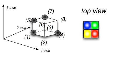
Figure 1: Unit cube with marked vertices. In the figure on the left-hand side, $\sigma^{(k)}=1$ only for $k=1,4,5,7$. The figure on the right-hand side represents the top view of the cube, where one of the four colors is assigned for each pair of ($\sigma^{(k)}$,$\sigma^{(k^{\prime})}$) aligned in the vertical direction. For example, red is assigned for $(\sigma^{(2)}=0$,$\sigma^{(6)}=0)$.

It is assumed that only one molecule can occupy each site in the cubic lattice $\Lambda=\{i\in{\bf N}^{3}|i=(i_{1},i_{2},i_{3}),1\leq i_{k}\leq L\}$. The total number of sites in the lattice is $N=L^{3}$. A molecule configuration is denoted by ${\boldsymbol{\sigma}}=(\sigma_{i})_{i\in\Lambda}$. For any nearest neighbor pair of sites $(i,j)$ that satisfies the relation $j-i=e_{k}$, where $e_{k}$ is the unit vector in the $k$ direction of the lattice, the interaction energy $V_{k}(\sigma,\sigma^{\prime})$ is defined for $(\sigma_{i},\sigma_{j})=(\sigma,\sigma^{\prime})$ as follows: $V_{k}(\sigma,\sigma^{\prime})=1$ when mark configurations in the adjacent plaquettes of unit cubes at sites $i$ and $j=i+e_{k}$ are different; otherwise, $V_{k}(\sigma,\sigma^{\prime})$ takes either $0$ or $-1$ irregularly. Such an irregular function was generated by selecting the value $0$ or $-1$ with probability $1/2$ for each case. The irregularity of $V$ is necessary to introduce a rugged energy landscape of LMCs. An example of the interaction energy is shown in Fig. 2. The Hamiltonian of the proposed model is given by

$$H({\boldsymbol{\sigma}})=\sum_{\langle i,j\rangle}V_{k}(\sigma_{i},\sigma_{j}),$$ (1)

where $\langle i,j\rangle$ represents a nearest neighbor pair of sites. Although some elements of the interaction energy are determined by using probabilities, a quenched disorder does not exist in the lattice. Indeed, $H({\boldsymbol{\sigma}})$ is translational invariant if the periodic boundary condition is assumed. Throughout this Letter, $\beta$ represents inverse temperature.

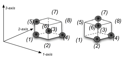
Figure 2: Example of the interaction energy. For two cubes $\sigma=29$ (left) and $\sigma^{\prime}=106$ (right), $V_{1}(\sigma,\sigma^{\prime})=1$, $V_{2}(\sigma,\sigma^{\prime})=1$, $V_{3}(\sigma,\sigma^{\prime})=1$, $V_{2}(\sigma^{\prime},\sigma)=1$, and $V_{3}(\sigma^{\prime},\sigma)=1$. $V_{1}(\sigma^{\prime},\sigma)$ is either $0$ or $-1$, which is selected with probability $1/2$.

Analysis

A molecule configuration without any mismatches between the mark configurations in all adjacent plaquettes is called a perfect matching configuration (PMC). The advantage of the proposed model is that all PMCs can be constructed using a simple iteration rule. The rule is as follows. First, the values of $\sigma_{i}^{(k)}$ for $k=1,2,3,4$ in plane $i_{3}=1$; for $k=1,2,5,6$ in plane $i_{2}=1$; and for $k=1,3,5,7$ in plane $i_{1}=1$ are randomly chosen. Then, the molecule type $\sigma_{i}$ for $i=(1,1,1)$ is determined. Accordingly, the value of $\sigma_{i}^{(8)}$ for $i=(1,1,1)$ is given and this value is equal to the value of $\sigma_{i}^{(7)}$ for $i=(2,1,1)$. Thus, the molecule type $\sigma_{i}$ for $i=(2,1,1)$ can be determined. By repeating this procedure, all the values of $\sigma_{i}$ for $i\in\Lambda$ can be determined depending on the initial choice of mark configurations in the planes. Since all PMCs are generated using the iteration rule, there are $2^{3L^{2}+3L+1}$ PMCs.

An important property of PMCs is that they exhibit neither long range positional order nor internal symmetry breaking. This property is evident from Fig. 3, where the cube configuration in plane $i_{3}=L/2$ is shown for a randomly chosen PMC. This configuration is certainly irregular. One can also examine this irregularity by measuring some statistical quantities. Theoretically, the irregularity may be understood from the deterministic iteration rule used for constructing PMCs. Although its rigorous proof is not obtained yet, one can demonstrate that the rule maintains the random nature of configurations in the planes $i_{1}=1$, $i_{2}=1$, and $i_{3}=1$ (See Ref. Sasa for a related argument.).

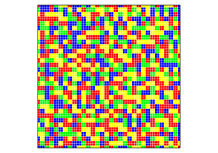
Figure 3: Perfect matching configuration $(L=32)$. Molecule configuration in plane $i_{3}=L/2$ is shown as the color representation of the top view of cubes. (See Fig. 1 for the color representation.)

Next, the energy landscape of $H({\boldsymbol{\sigma}})$ is discussed. It can be easily confirmed that the replacement of any cube in a PMC always increases the energy. That is, all PMCs are LMCs. Moreover, LMCs other than PMCs exist. Suppose that a cube at site $i$ in a PMC is altered such that either $\sigma_{i}^{(6)}$ or $\sigma_{i}^{(7)}$ is changed. Then, three mismatches of $\sigma_{i}$ are generated in the configuration. Two of them can be eliminated by employing the iteration rule beginning from the cube next to $\sigma_{i}$. This leads to an LMC with one mismatch which cannot be eliminated by any finite number of steps of cube replacement in the thermodynamic limit. The repetition of this procedure can yield LMCs with $k$ isolated mismatches which cannot be eliminated by any finite number of steps of cube replacement in the thermodynamic limit, where $k$ is an arbitrary finite integer. A collection of all such LMCs is denoted by $({\boldsymbol{\sigma}}^{\alpha})_{\alpha\in{\cal A}}$, where ${\cal A}$ is the index set. $|{\cal A}|$ is not estimated, but from the construction method of LMCs, it is found that $|{\cal A}|\simeq\exp(s_{0}N)$, where $s_{0}$ is a positive constant.

Since the energy density $u_{\alpha}\equiv H({\boldsymbol{\sigma}}^{\alpha})/N$ for $\alpha\in{\cal A}$ is obtained as the space average of interaction energies for an irregular configuration ${\boldsymbol{\sigma}}^{\alpha}$, the distribution of $u_{\alpha}$ has a sharp peak with width of $O(1/\sqrt{N})$. Thus, as studied in the random energy model REM , it is expected for sufficiently low temperature that the statistical measure condensates onto configurations near a ${\boldsymbol{\sigma}}^{\alpha}$ satisfying $H({\boldsymbol{\sigma}}^{\alpha})\simeq u_{*}N$, where $u_{*}$ is the minimum energy density of LMCs in the thermodynamic limit. This condensation phenomenon leads to MOSIC. ”

Numerical experiments

The condensation phenomenon is explored by numerical experiments. The statistical quantities for rather small-size systems in the equilibrium state under free boundary conditions are calculated by employing the exchange Monte Carlo method HukushimaNemoto .

First, thermodynamic quantities for the proposed model are investigated. As an example, in the left side of Fig. 4, the change in the energy density $u=\langle\hat{u}\rangle$ with inverse temperature $\beta$ is shown for $L=8,9,10,11$, where $\hat{u}=H({\boldsymbol{\sigma}})/N$. An abrupt drop is observed around a temperature for each $L$. Since $-du/d\beta$ is equal to the intensity of energy fluctuations $\chi_{u}=N\langle(\hat{u}-u)^{2}\rangle$, $\chi_{u}$ is displayed in the right side of Fig. 4. The peak value of $\chi_{u}$, denoted by $\chi_{u}^{\rm max}$, increases as $\chi_{u}^{\rm max}\simeq L^{4.7}$ (see Fig. 5), which is faster than $\chi_{u}^{\rm max}\simeq L^{3}$ expected for the first-order transition. Furthermore, two graphs of $\chi_{u}$ for $L=11$ and $L=10$ in Fig. 4 satisfy a relation

$$\chi_{u}\simeq L^{\alpha/\nu}f((\beta-\beta_{\rm c}(L))L^{1/\nu}),$$ (2)

where $\alpha=1.0$ and $\nu=1/4.7\simeq 0.21$. $\beta_{\rm c}(L)$ is estimated as the value of $\beta$ where $\chi_{u}$ becomes maximum. From these results, it is certain that a thermodynamic transition occurs at a non-zero temperature in the thermodynamic limit, and it may be conjectured that the transition is the first order. It should be noted that the system sizes in the experiment are too small to identify the nature of the transition precisely.

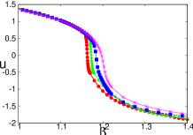
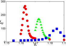
Figure 4: (Color online) Thermodynamic quantities for several values of $L$. The left figure shows the energy density $u$ as functions of $\beta$ for $L=8$ (asterisk), 9 (square), 10 (triangle) and $11$ (circle). The intensity of energy fluctuations is displayed in the right side. $L=9$ (square), 10 (triangle) and $11$ (circle).

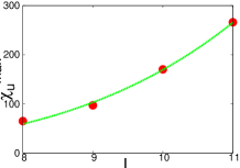
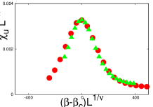
Figure 5: (Color online) The left graph indicates the maximum value of $\chi_{u}$ for $L$. The guide line represents $\chi_{u}=(L/3.4)^{4.7}$. The right figure shows $\chi_{u}L^{-4.7}$ versus $(\beta-\beta_{\rm c}(L))L^{4.7}$ for two graphs with $L=10$ and $L=11$.

Next, in order to observe MOSIC in low temperatures, two independent identical systems are prepared, where two configurations are denoted by $(\sigma^{(1)}_{i})_{i\in\Lambda}$ and $(\sigma^{(2)}_{i})_{i\in\Lambda}$, respectively. The overlap between the two configurations is defined as

$$\hat{q}\equiv\frac{1}{N}\sum_{i\in\Lambda}\delta(\sigma_{i}^{(1)},\sigma_{i}^{(2)}).$$ (3)

Let $P(q,\beta)$ be the distribution function of $\hat{q}=q$ in the equilibrium state of the system with inverse temperature $\beta$. In Fig. 6, the color representation of $\log P(q,\beta)$ is shown, which clearly indicates the existence of two peaks at low temperatures. Since typical configurations in low-temperatures are irregular, it is concluded that MOSIC emerges. This is the most remarkable result in this Letter.

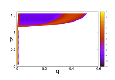
Figure 6: A color representation of $\log P$ as a function of $q$ for different values of $\beta$. $L=10$.

A further evidence of MOSIC is proposed by studying the system under a special boundary configuration, where molecules in the boundary planes $i_{k}=1$ and $i_{k}=L$ ($k=1,2,3)$ are fixed as those of ${\boldsymbol{\sigma}}^{*}$ chosen from equilibrium configurations with large $\beta$. Then, as shown in the left side of Fig. 7, the overlap with ${\boldsymbol{\sigma}}^{*}$, which is characterized by

$$q_{*}=\frac{1}{\tilde{N}}\sum_{i\in\tilde{\Lambda}}\langle\delta(\sigma_{i},\sigma_{i}^{*})\rangle,$$ (4)

approaches one as $\beta$ is increased, where $\tilde{\Lambda}$ represents the inner region except for the boundaries in $\Lambda$. $\tilde{N}=(L-2)^{3}$ is the number of sites in $\tilde{\Lambda}$. The result indicates that the boundary configuration selects one irregular configuration, just as the spin-up boundary configuration determines the ordered phase with positive magnetization. This is a direct evidence that there exists a low-temperature phase with MOSIC.

Finally, properties near the transition point are briefly studied from a viewpoint of dynamics. The simplest quantity characterizing dynamical behaviors is the correlation function

$$C_{q}(t)=\frac{1}{N}\sum_{i\in\Lambda}\langle\delta(\sigma_{i}(t),\sigma_{i}(0))\rangle-\frac{1}{128},$$ (5)

where $\sigma_{i}(0)$ is sampled in the equilibrium state and the time evolution $\sigma(t)$ obeys the Glauber dynamics with the heat bath method. It is observed that $C_{q}(t)$ decreases exponentially in sufficiently high temperature, while it saturates to a finite value in the low temperature phase. Near the transition point, two types of trajectories, which correspond to de-correlation and freezing, coexist. The behavior may be consistent with the discontinuous transition of $q$. Here, as shown in the right side of Fig. 7, no intermediate plateau is observed, in contrast to the RFOT scenario. Although the decay of $C_{q}(t)$ becomes slower as $\beta$ approaches the transition point on the high temperature side, the divergent behavior is not concluded in the experiment of the small size system.

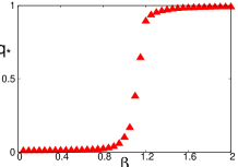
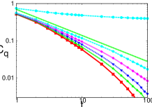
Figure 7: (Color online) The left-side figure shows $q_{*}$ as a function of $\beta$ $(L=10)$. In the right side, $C_{q}(t)$ are plotted with a log-log scale. $\beta=1.15$ (squares), $1.155$ (upward triangles), $1.16$ (downward triangles), $1.165$ (diamonds), and $1.17$ (circles). Since trajectories for $\beta=1.17$ are clearly classified into two groups, two graphs corresponding to the two groups are plotted. The dotted straight line represents a power-law form $C_{q}(t)=0.7t^{-0.7}$ as a guide line.

Concluding Remarks

In this Letter, a pure glass model in finite dimensions has been proposed. In this model, typical equilibrium configurations in low temperature have macroscopic overlaps with one of some special irregular configurations. Although the behavior is similar to that observed in the models that exhibits one step replica symmetry breaking, the nature of the transition seems to be different from the RFOT. In contrast to previous numerical studies on glass transition in finite dimensions Rieger ; Ritort ; FZ , the present work has explored the nature of the low temperature phase more than properties near the transition point. The two peaks in $P(q)$ in low temperatures may be the clearest demonstration among all existing studies of glassy systems in finite dimensions. Furthermore, the construction of an infinite series of local minimum configurations will provide a clue for theoretical analysis of statistical mechanics in sufficiently low temperatures.

Before ending the Letter, I provide a few remarks. The arguments presented in this Letter are based on several conjectures whose validity is demonstrated with the aid of numerical experiments. A complete theory for describing pure glass will be developed in future work. Then, it may be significant to construct a simpler model that exhibits a behavior similar to that of pure glass. Furthermore, it is interesting to consider an effective field theory for describing pure glass, which might be related to the replica field theory rft .

The ultimate goal of this study is to construct a pure glass experimentally. Toward this goal, the next subject is to study a Hamiltonian system for which the rugged energy landscape may be discussed theoretically. It will be amazing to observe the properties of pure glass via molecular dynamics simulations. In this study, complicated shapes of molecules will be employed so as to produce interaction potentials similar to $V_{k}(\sigma,\sigma^{\prime})$. This challenge may be related to recent studies on complex structures emerging out of designed building blocks with anisotropy Glotzer ; Granick . Here, let us recall a history of quasi-crystals. The mathematical study on aperiodic but regular tiling was conducted in the 1960s wtile , whereas the experimental construction of quasi-crystals was first reported in 1984 QC-exp . As an extension of this Letter, a theoretical study on irregular but ordered tiling will be conducted. I hope that future researchers will attempt to consider the possibility of constructing pure glass experimentally.

The author thanks K. Hukushima, N. Mitarai, H. Ohta, H. Tasaki and H. Yoshino for helpful discussions. The present study was supported by KAKENHI Nos. 22340109 and 23654130, and the JSPS Core-to-Core Program “International research network for non-equilibrium dynamics of soft matter”.

References

- (1) T. R. Kirkpatrick, D. Thirumalai, and P. G. Wolynes, Phys. Rev. A 40, 1045 (1989).
- (2) M. Mézard and G. Parisi, Phys. Rev. Lett. 82, 747 (1999).
- (3) G. Parisi and F. Zamponi, Rev. Mod. Phys. 82, 789 (2010).
- (4) G. Biroli and J.-P. Bouchaud, arXiv:0912.2542 (2009).
- (5) W. Kauzmann, Chem.Rev. 43, 219 (1948).
- (6) C. Cammarota, G. Biroli, M. Tarzia, and G. Tajus, Phys. Rev. Lett. 106, 115705 (2011).
- (7) J. Yeo and M. A. Moore, Phys. Rev. B 85, 100405(R) (2012).
- (8) G. Biroli and M. Mézard, Phys. Rev. Lett. 88, 025501 (2001).
- (9) M. P. Ciamarra, M. Tarzia, A. de Candia, and A. Coniglio, Phys. Rev. E. 67, 057105 (2003).
- (10) F. Krzakala, M. Tarzia, L. Zdeborová, Phys. Rev. Lett. 101, 165702, (2008).
- (11) S. Franz, Europhys. Lett. 73, 492 (2006).
- (12) S. Franz and A. Montanari, J. Phys. A: Math. Theor. 40, F251 (2007).
- (13) W. Götze, Complex Dynamics of Glass-Forming Liquids (Oxford University Press, Oxford, 2009).
- (14) B. Grünbaum and G. C. Shephard, Tilings and Patterns (W. H. Freeman and Company, New York, 1987).
- (15) R. M. Robinson, Inventions Math. 12, 177 (1971).
- (16) S.-I. Sasa, J. Phys. A: Math. Theor. 45, 035002 (2012).
- (17) B. Derrida, Phys. Rev. B 24, 2613 (1981).
- (18) K. Hukushima and K. Nemoto, J. Phys. Soc. Jpn. 65, 1604 (1996).
- (19) H. Rieger, Physica A 184, 279 (1992).
- (20) D. Alvarez, S. Franz, F. Ritort, Phys. Rev. B 54, 9756 (1996).
- (21) F. Krzakala and L. Zdeborova, J. Chem. Phys. 134, 034513 (2011).
- (22) F. Caltagirone, U. Ferrari, L. Leuzzi, G. Parisi, and T. Rizzo Phys. Rev. B 83, 104202 (2011).
- (23) S. C. Glotzer and M. J. Solomon, Nat. Mater. 6, 557 (2007).
- (24) Q. Chen, S. C. Bae, and S. Granick, Nature 469, 381 (2011).
- (25) D. Shechtman, I. Blech, D. Gratias, and J. W. Cahn, Phys. Rev. Lett. 53, 1951 (1984).