High-Performance Numerical Library for Solving Eigenvalue Problems

Eric Polizzi Research Lab.
Department of Electrical and Computer Engineering,
Department of Mathematics and Statistics,
University of Massachusetts, Amherst

References

If you are using FEAST, please consider citing one or more publications below in your work.

Main reference

E. Polizzi, Density-Matrix-Based Algorithms for Solving Eigenvalue Problems,
Phys. Rev. B. Vol. 79, 115112 (2009)

Math analysis

P. Tang, E. Polizzi, FEAST as a Subspace Iteration EigenSolver Accelerated by Approximate Spectral Projection; SIAM Journal on Matrix Analysis and Applications (SIMAX) 35(2), 354–390 - (2014)

Non-Hermitian solver

J. Kestyn, E. Polizzi, P. T. P. Tang, FEAST Eigensolver for Non-Hermitian Problems,
arxiv.org/abs/1506.04463 (2015)

Hermitian using Zolotarev quadrature

S. Güttel, E. Polizzi, P. T. P. Tang, G. Viaud, Optimized Quadrature Rules and Load Balancing for the FEAST Eigenvalue Solver,
SIAM Journal on Scientific Computing (SISC), to appear (2015), arxiv.org/abs/1407.8078 (2014)

Eigenvalue count using stochastic estimates

E. Di Napoli, E. Polizzi, Y. Saad, Efficient Estimation of Eigenvalue Counts in an Interval,
arxiv.org/abs/1308.4275 (2015)

Contact

If you have any questions or feedback regarding FEAST, please send an-email to feastsolver@gmail.com.

FEAST algorithm and software team, collaborators and contributors

		Algorithm and research	Software development
	Eric Polizzi	Lead	v3.0, v2.1, v2.0, v1.0
	James Kestyn	Non-Hermitian FEAST	v3.0
UMass		improved schemes, tunings, tools	FEAST non-Hermitian upgrade
Amherst	Brendan Gavin	Non-linear eigenvector problem
Team		expanded subspace scheme
	Braegan Spring	SPIKE-SMP v1.0	v3.0
		scalable banded system solver	FEAST banded interfaces upgrade
	Peter Tang	General FEAST algorithm analysis
	Intel	improved schemes
Collaborators	Yousef Saad	Eigenvalue count estimates
&	U. of Minnesota	new FEAST schemes (in progress)
Contributors	Edoardo Di Napoli	Eigenvalue count estimates
	Jülich Supercomput.
	Stefan Güttel	Zolotarev quadrature & analysis	v3.0
	Manchester U.		Zolotarev quadrature database
	Gautier Viaud	Zolotarev quadrature & analysis
	ECP France
	Ahmed Sameh	SPIKE-SMP v1.0
	Purdue U.	SVD-FEAST (in progress)

Chapter 1 Table of Contents

toc

1 Updates/Upgrades Summary

If you are a FEAST’s first time user, you can skip this section.

Here is a summary of the most important updates/upgrades.

1.1 From v2.1 to v3.0

• A variety of new features have been added in v3.0. This includes support for non-Hermitian matrices, elliptical contours and custom user-defined contours, stochastic estimates for the number of eigenvalues inside search interval, and different quadrature rules. Many new routines have been added. See Table 1 for a summary.

Family of Eigenvalue Problems	Routines in v3.0
$AX=BX\Lambda$
$A^{H}\widehat{X}=B^{H}\widehat{X}\Lambda^{*}$	Elliptical Contours (Standard)	Custom Contour (Expert)
Real and Symmetric	{s,d}feast_srci	{s,d}feast_srcix
$A=A^{T}$, $B$ spd, $X=\widehat{X}$ real, $\Lambda$ real	{s,d}feast_{sy,sb,scsr}{ev,gv}	{s,d}feast_{sy,sb,scsr}{ev,gv}x
Complex and Hermitian	{c,z}feast_hrci	{c,z}feast_hrcix
$A=A^{H}$, $B$ hpd, $X=\widehat{X}$ complex, $\Lambda$ real	{c,z}feast_{he,hb,hcsr}{ev,gv}	{c,z}feast_{he,hb,hcsr}{ev,gv}x
Complex and Symmetric	{c,z}feast_srci	{c,z}feast_srcix
$A=A^{T}$, $B=B^{T}$, $X=\widehat{X}^{*}$ complex, $\Lambda$ complex	{c,z}feast_{sy,sb,scsr}{ev,gv}	{c,z}feast_{sy,sb,scsr}{ev,gv}x
Real and Non-Symmetric	{s,d}feast_grci	{s,d}feast_grcix
$A,B$ general, $X\neq\widehat{X}$ complex, $\Lambda$ complex	{s,d}feast_{ge,gb,gcsr}{ev,gv}	{s,d}feast_{ge,gb,gcsr}{ev,gv}x
Complex and General	{c,z}feast_grci	{c,z}feast_grcix
$A,B$ general, $X\neq\widehat{X}$ complex, $\Lambda$ complex	{c,z}feast_{ge,gb,gcsr}{ev,gv}	{c,z}feast_{ge,gb,gcsr}{ev,gv}x

Table 1: Summary of all routines in FEAST v3.0 (140 total) - new routines in red

• Non-Hermitian routines use a different variant of the FEAST algorithm than Hermitian cases. The major difference is the use of dual subspaces, $Q$ and $\widehat{Q}$, corresponding to Right $X$ and Left $\widehat{X}$ eigenvectors. Also, the search interval must become 2-dimensional to account for complex eigenvalues. More detail is given in:

  FEAST Eigensolver for Non-Hermitian Problems,
  J. Kestyn, E. Polizzi, P. Tang, http://arxiv.org/abs/1506.04463 (2015)

• FEAST now offers multiple quadrature rules: Gauss, Trapezoidal and Zolotarev (for the Hermitian case), as well as elliptical complex contour. More detail is given in:

  Optimized Quadrature Rules and Load Balancing for the FEAST Eigenvalue Solver,
  S. Güttel, E. Polizzi, P. T. Tang, G. Viaud, http://arxiv.org/abs/1407.8078

• All FEAST routines can be called within their “expert mode” version which features new user input lists for nodes and weights.

• Stochastic estimates for the number of eigenvalues inside of the search interval are now available. This feature can help users in estimating a value for the search subspace $M_{0}$. Refer to the following publication for more information.

  Efficient Estimation of Eigenvalue Counts in an Interval,
  E. Di Napoli , E. Polizzi, Y. Saad, http://arxiv.org/abs/1308.4275

• Various utility routines have also been added (see section 6). We note in particular the possibility for the users to design their own contour shape in the complex plane. This is particularly helpful for non-Hermitian routines as it grants flexibility in targeting specific eigenvalues. See Section 6 for additional information.

• FEAST PARAMETERS- new or updated fpm parameters:

  • fpm(2) is updated- inludes more options for #nodes in the half-contour (for Hermitian FEAST)
    If fpm(16)=0,2, values permitted $[1\mbox{ to }20,24,32,40,48,56]$
    If fpm(16)=1, all values permitted

  • fpm(6) is updated- default value changed to 1 -
    Convergence criteria on trace (0) or eigenvectors relative residual (1)

  • fpm(8) is added - Total number of contour integration nodes (i.e. complex shifts) for non-Hermitian FEAST.
    If fpm(17)=0, values permitted $[2\mbox{ to }40,48,64,80,96,112]$
    If fpm(17)=1, all values permitted
    Remark: fpm(8) represents the #nodes for the full contour while fpm(2) represents the #nodes for the half-contour used by Hermitian FEAST.

  • fpm(10) is added - can be used with the FEAST predefined driver interfaces (0: default, 1: store all the linear system factorizations).
    Remark: (i) storing the factorizations will significantly improve the performances (for FEAST DENSE in particular), but can significantly increase the memory usage; (ii) option 1 works with FEAST-MPI as well - store all factors associated to a given mpi process

  • fpm(14) is modified - include option 2
    0- default normal FEAST execution
    1- return only subspace Q size M0 after 1 contour
    2- return stochastic estimates of the #eigenvalue (in argument ’M’ and ’res’ for running average)

  • fpm(16) is added - Integration type for symmetric (0: Gauss/Default, 1: Trapezoidal, 2: Zolotarev)

  • fpm(17) is added - Integration type for non-symmetric (0: Gauss, 1: Trapezoidal/Default)

  • fpm(18) is added - Ratio for ellipsoid contour - fpm(18)/100 is ratio ’vertical axis’/’horizontal axis’ of the ellipse using the definition of the search contour. For example:
    value 100 is the default (circle);
    value 50 will create a 50% flat ellipse;
    value 200 will create a 200% tall ellipse.

  • fpm(19) is added - Rotation angle in degree [-180:180] for Ellipsoid contour and using FEAST non-Hermitian- Origin of the rotation is the vertical axis.

2 Preliminary

“The solution of the algebraic eigenvalue problem has for long had a particular fascination for me because it illustrates so well the difference between what might be termed classical mathematics and practical numerical analysis. The eigenvalue problem has a deceptively simple formulation and the background theory has been known for many years; yet the determination of accurate solutions presents a wide variety of challenging problems.”
J. H. Wilkinson- The Algebraic Eigenvalue Problem- 1965

In his seminal textbook, J. H. Wilkinson artfully outlined the fundamentals, difficulties and numerical challenges for addressing the eigenvalue problem. Since then, the eigenvalue problem has led to many challenging numerical questions and a central problem: how can we compute eigenvalues and eigenvectors in an efficient manner and how accurate are they?

In many modern science and engineering applications, especially for those where the underlying system matrices are large and sparse, it is often the case that only selected segments of the eigenvalue spectrum are of interest. Although extensive efforts have been devoted to develop new numerical algorithms and library packages, they are all commonly facing new challenges for addressing the current large-scale simulations needs for ever higher level of accuracy, robustness and scalability on modern parallel architectures. The FEAST eigensolver library package is intended to uniquely address all those issues. Its originality lies with a new transformative numerical approach to the traditional eigenvalue algorithm design - the FEAST algorithm.

2.1 The FEAST Algorithm

Unlike any other eigenvalue numerical software, the FEAST solver is based on a new algorithm which deviates fundamentally from the Krylov subspace based techniques (Arnoldi and Lanczos algorithms), Davidson-Jacobi techniques or other traditional subspace iteration techniques. The FEAST algorithm is a general purpose eigenvalue solver which takes its inspiration from the density-matrix representation and contour integration technique in quantum mechanics. FEAST can be used for solving the generalized eigenvalue problem ${AX}={BX}\Lambda$ (Hermitian or non-Hermitian), and obtaining all the eigenvalues $\lambda$ and (left/right) eigenvectors within a given search interval $[\lambda_{min},\lambda_{max}]$ or an arbitrary contour in the complex plane. FEAST’s main building block is a numerical quadrature computation i.e. ${Q}=\sum w_{j}{Q_{j}}$, consisting of solving independent linear systems along a complex contour i.e. $(z_{j}{B}-{A}){Q_{j}}={Y}$ (with $z_{j}$ quadrature node), each with multiple right hand sides ${Y}$. A Rayleigh-Ritz procedure is then used to generate a reduced dense eigenvalue problem orders of magnitude smaller than the original one (the size of this reduced problem is of the order of the number of eigenpairs inside the search interval/contour). The algorithm contains elements from complex analysis, numerical linear algebra and approximation theory, to produce an optimal subspace iteration method using spectral projectors. Not only the FEAST algorithm features some unique and remarkable convergence and robustness properties, it can exploit a key strength of modern computer architectures, namely, multiple levels of parallelism. All the important intrinsic properties of the algorithm, which have been analyzed and commented at length in publications, can be summarized as follows:

• all multiplicities are naturally captured;

• no explicit orthogonalization procedure on long vectors is required;

• reusable subspace capable to generate suitable initial guess;

• allows the use of iterative methods for solving large-sparse linear systems;

• can exploit natural parallelism at three different levels:

  1. search intervals can be treated separately (no overlap);

  2. linear systems can be solved independently across the quadrature nodes of the complex contour;

  3. each complex linear system with multiple right-hand-sides can be solved in parallel.

  Consequently, within a parallel environment, the algorithm complexity depends on solving a single linear system.

2.2 The FEAST Solver Package version v3.0 

The FEAST numerical library package (www.feast-solver.org) has first been developed and released (under free BSD license) in Sep. 2009 (v1.0), follows by upgrades in Mar. 2012 (v2.0), and Feb. 2013 (v2.1) [version adopted by Intel-MKL]. The current version of the FEAST package (v3.0) released in Jun. 2015, focuses on solving the Hermitian and Non-Hermitian eigenvalue problems (real symmetric, real non-symmetric, complex Hermitian, complex non-Hermitian, complex symmetric) on both shared-memory architecture (i.e. FEAST-SMP version) and distributed architecture (i.e. FEAST-MPI version including the three levels of parallelism MPI-MPI-OpenMP).

FEAST is a comprehensive numerical library offering both simplicity and flexibility, and packaged around a “black-box” interface as depicted in Figure 1.

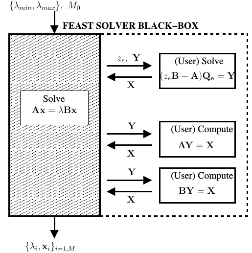
Figure 1: “Black-box” interface for the Hermitian problem. FEAST requires a search interval and a search subspace size $M_{0}$. It includes features such as reverse communication interfaces (RCI) that are matrix format independent, and linear system solver independent, as well as ready to use predefined interfaces for dense, banded and sparse systems. For the predefined interfaces case the “black-box” region extends then to the right dashed box, and only the system matrices are required as inputs from the users. The RCI interfaces represent the kernel of FEAST which can be customized by the users to allow maximum flexibility for their specific applications. Users have then the possibility to integrate their own linear system solvers (direct or iterative – with or without preconditioner) and handle their own matrix-vector multiplication procedure.

The current main features of the FEAST package include:

• Standard or generalized Hermitian and non-Hermitian eigenvalue problems (left/right eigenvectors and bi-orthonormal basis);

• Two libraries: SMP version (one node), and MPI version (multi-nodes);

• Real/Complex arithmetic and Single/Double precisions;

• A set of flexible and useful practical options (quadrature rules, contour shapes, stopping criteria, initial guess, etc.)

• Fast stochastic estimates for search subspace size $M_{0}$.

• Source code and pre-compiled libraries provided for common architectures (e.g. x64)- FEAST is written in Fortran 90, but the FEAST libraries do not contain Fortran runtime dependencies to maximize portability (e.g. compatibility with any Fortran or C compilers).

• Reverse communication interfaces (RCI): Maximum flexibility for application specific. Those are matrix format independent, inner system solver independent, so users must provide their own linear system solvers (direct or iterative) and mat-vec utility routines.

• Predefined driver interfaces for dense, banded, and sparse (CSR) formats: Less flexibility but easy to use (”plug and play”):

  • FEAST_DENSE interfaces require LAPACK.

  • FEAST_BANDED interfaces use the SPIKE-SMP linear system solver (included)

  • FEAST_SPARSE interfaces requires the Intel MKL-PARDISO solver.

• All the FEAST interfaces require (any optimized) LAPACK and BLAS packages.

• Multiple utility routines are also included (e.g. user-defined custom contour in complex plane, variation of the spectral projector rational function, extract nodes/weights from predefined quadrature rules, etc.)

• Examples and documentation included,

• Utility sparse drivers included (i.e. users can also provide their matrix systems in coordinate/matrix-market format for testing, timing, etc.).

Remark: Although it could be possible to develop a large collection of FEAST drivers that can be linked with all the main linear system solver packages, we are rather focusing our efforts on the development of highly efficient, functional and flexible FEAST RCI interfaces which are placed on top of the computational hierarchy. Within the FEAST RCI interfaces, maximum flexibility is indeed available to the users for choosing their preferred and/or application specific direct linear system method or iterative method with (customized or generic) preconditioner.

2.2.1 Using the FEAST-SMP version

For a given search interval, parallelism (via shared memory programming) is not explicitly implemented in FEAST i.e. the inner linear systems are solved one after another within one node (avoid the fight for resources). Therefore, parallelism can only be achieved if the inner system solver and the mat-vec routines are threaded. Using the FEAST predefined drivers, in particular, parallelism is implicitly obtained within the shared memory version of BLAS, LAPACK, SPIKE-SMP or MKL-PARDISO. If FEAST is linked with the INTEL-MKL library, the shell variable MKL_NUM_THREADS can be used for setting automatically the number of threads (cores) for both BLAS, LAPACK and MKL-PARDISO. In the general case, the user is responsible for activated the threaded capabilities of their BLAS, LAPACK libraries and their own linear systems solvers - most likely using the shell variable OMP_NUM_THREADS. The latter must be defined with the FEAST-BANDED interfaces since they are already making use of our own SPIKE-SMP solver.

Remark: If memory resource is not an issue (in particular for small to moderate size systems), the flag fpm(10) should be changed to value 1. In this case, all the factorizations performed by the FEAST predefined drivers (dense, banded, sparse) will be saved into memory (i.e. they are not recomputed along the FEAST iterations) and performances will improved. With this option the FEAST-DENSE interface, in particular, should become more competitive in comparison with the LAPACK eigenvalue routines for computing selected eigenpairs.

2.2.2 Using the FEAST-MPI version

In the current FEAST version, only the second-level of parallelism is explicitly addressed by the code. This is accomplished in a trivial fashion by sending off the different linear systems (which can be solved independently for the points along the complex contour) along the compute nodes. From the user perspective, interfaces and arguments list stay completely unchanged and it is the -lpfeast, etc. library (instead of -lfeast, etc.) that needs to be linked within an MPI environment. Although, FEAST can run on any numbers of MPI processors, there will be a peak of performance if the number of MPI processes is equal to the number of contour points i.e. either fpm(2) or fpm(8) depending on the nature the eigenvalue problem and the FEAST drivers. Indeed, the MPI implementation in v3.0 does not yet provide an option for the third level of parallelism (system solver level) and FEAST still needs to call a shared-memory solver. However, it is important to note that a MPI-level management has been added to allow easy parallelism of the search interval using a coarser level of MPI (i.e. first level parallelism). For this case, a new flag fpm(9) has been added as the only new input required by FEAST. This flag can be set equal to a new local communicator variable “MPI_COMM_WORLD” which contains the selected user’s MPI processes for a given search interval. If only one search interval is used, this new flag is set by default to the global “MPI_COMM_WORLD” value in the FEAST initialization step.

2.3 Installation and Setup: A Step by Step Procedure

In this section, we address the following question: How should you install and link the FEAST library?

2.3.1 Installation- Compilation

Please follow the following steps (for Linux/Unix systems):

1. Download the latest FEAST version in http://www.ecs.umass.edu/$\sim$polizzi/feast, for example, let us call this package feast_3.0.tgz.

2. Put the file in your preferred directory such as $HOME directory or (for example) /opt/ directory if you have ROOT privilege.

3. Execute: tar -xzvf feast_3.0.tgz; Figure 2 represents the main FEAST tree directory being created.

   ⬇

   FEAST

   |

   3.0

   |

   ————————————————————–

   | | | | | |

   doc example include lib src utility

   | | | |

   ——- ——– ——- —–

   |-Hermitian |-x64 |-kernel |-SMP

   |-Non-Hermitian |-dense |-MPI

   |-banded |-data

   |-sparse

   
   

   Figure 2: Main FEAST tree directory.

4. let us denote <FEAST directory> the package’s main directory after installation. For example, it could be

   $\sim$/home/FEAST/3.0    or    /opt/FEAST/3.0.

   It is not mandatory but recommended to define the Shell variable $FEASTROOT, e.g.

   export FEASTROOT=<FEAST directory> 
   or   set FEASTROOT=<FEAST directory> 

   respectively for the BASH or CSH shells. One of this command can be placed in the appropriate shell startup file in $HOME (i.e .bashrc or .cshrc).

5. The FEAST pre-compiled libraries can be found at

   $FEASTROOT/lib/<arch> 

   where <arch>  denotes the computer architecture. Currently, the following architectures are provided:

   • x64 for common 64 bits architectures (e.g. Intel em64t: Nehalem, Xeon, Pentium, Centrino etc.; amd64),

   The pre-compiled libraries are free from Fortran90 runtime dependencies (i.e. they can be called from any Fortran or C codes without compatibility issues). For the FEAST-MPI, the precompiled library include two versions MPICH2 and OpenMPI. If your current architecture is listed above, you can proceed directly to step 7, if not, you will need to compile the FEAST library in the next step. You would also need to compile FEAST-MPI if you are using a different MPI implementation that the one proposed here.

6. Compilation of the FEAST library source code:

   • Go to the directory $FEASTROOT/src

   • Edit the make.inc file, and follow the directions. Depending on your options, you would need to change appropriately the name/path of the Fortran90 or/and C Compilers and optionally MPI.

     Two main options are possible:

     1. FEAST is written in Fortran90 so direct compilation is possible using any Fortran90 compilers (tested with ifort and gfortran). If this option is selected, users must then be aware of runtime dependency problems. For example, if the FEAST library is compiled using ifort but the user code is compiled using gfortran or C then the flag -lifcoremt should be added to this latter; In contrast, if the FEAST library is compiled using gfortran but the user code is compiled using ifort or C, the flag -lgfortran should be used instead.

     2. Compilation free from Fortran90 runtime dependencies (i.e. some low-level Fortran intrinsic functions are replaced by C ones). This is the best option since once compiled, the library could be called from any Fortran or C codes removing compatibility issues. This compilation can be performed using any C compilers (gcc for example), but it currently does require the use of the Intel Fortran Compiler.

     The same source codes are used for compiling FEAST-SMP and/or FEAST-MPI. For this latter, the MPI instructions are then activated by compiler directives (a flag <-DMPI> is added). The user is also free to choose any MPI implementations (tested with Intel-MPI, MPICH2 and OpenMPI).

   • For creating the FEAST-SMP: Execute:
     make ARCH=<arch>  LIB=feast all
     where <arch>  is your selected name for your architecture; your FEAST library including:
     libfeast_sparse.a
     libfeast_banded.a
     libfeast_dense.a
     libfeast.a
     will then be created in $FEASTROOT/lib/<arch>  .

   • Alternatively, for creating the FEAST-MPI library: Execute:
     make ARCH=<arch>  LIB=pfeast all to obtain:
     libpfeast_sparse.a
     libpfeast_banded.a
     libpfeast_dense.a
     libpfeast.a
     You may want to rename these libraries with a particular extension name associated with your MPI compilation.

7. Congratulations, FEAST is now installed successfully on your computer !!

   2.3.2 Linking FEAST

   In order to use the FEAST library for your F77, F90, C or MPI application, you will then need to add the following instructions in your Makefile:

   • for the LIBRARY PATH:   -L/$FEASTROOT/lib/<arch> 

   • for the LIBRARY LINKS using FEAST-SMP: (examples)
     -lfeast (FEAST kernel alone - Reverse Communication Interfaces)
     -lfeast_dense -lfeast (FEAST dense interfaces)
     -lfeast_banded -lfeast (FEAST banded interfaces)
     -lfeast_sparse -lfeast (FEAST sparse interfaces)
     -lfeast_sparse -lfeast_banded -lfeast (FEAST sparse and banded interfaces)

   • for the LIBRARY LINKS using FEAST-MPI:(examples)
     -lpfeast<ext> (FEAST kernel alone - Reverse Communication Interfaces)
     -lpfeast_dense<ext> -lpfeast<ext> (FEAST dense interfaces)
     -lpfeast_banded<ext> -lpfeast<ext> (FEAST banded interfaces)
     -lpfeast_sparse<ext> -lpfeast<ext> (FEAST sparse interfaces)
     -lpfeast_sparse<ext> -lpfeast_banded<ext> -lpfeast<ext> (FEAST sparse and banded interfaces)
     where, in the precompiled library, <ext> is the extension name associated with _impi, _mpich2 or _openmpi respectively for Intel MPI, MPICH2 and OpenMPI.
     

     In order to illustrate how should one use the above FEAST library links including dependencies, let us call (for example) -llapack, -lblas respectively your link for the your optimized LAPACK and BLAS packages. The complete library links with dependencies are then given for FEAST-SMP or FEAST-MPI by (examples):
     -l<p>feast -l<yourownsystemsolver> -llapack -lblas
     -l<p>feast_dense -lfeast -llapack -lblas
     -l<p>feast_banded -lfeast -llapack -lblas
     

     Remarks
     1- -l<yourownsystemsolver> represents the link to your own system solver in Figure 1.
     2- If -lfeast_sparse or -lpfeast_sparse<ext> are used, they must be linked with Intel MKL (which contains both MKL_PARDISO, LAPACK and BLAS)
     

   • for the INCLUDE PATH:   -I/$(FEASTROOT)/include
     It is mandatory only for C codes. Additionally, instructions need to be added in the header C file (all that apply):
     #include "feast.h"
     #include "feast_sparse.h"
     #include "feast_banded.h"
     #include "feast_dense.h"

2.4 A simple “Hello World” Example (F90, C, MPI-F90, MPI-C)

This example solves a 2-by-2 dense standard eigenvalue system $\bf Ax=\lambda x$ where

$${\bf A}=\begin{pmatrix}2&-1\\ -1&2\end{pmatrix}$$ (1)

and the two eigenvalue solutions are known to be $\lambda_{1}=1$, $\lambda_{2}=3$ which can be associated respectively with the orthonormal eigenvectors $(\sqrt{2}/2,\sqrt{2}/2)$ and $(\sqrt{2}/2,-\sqrt{2}/2)$.

Let us suppose that one can specify a search interval, a single call to the DFEAST_SYEV subroutine solves then this dense standard eigenvalue system in double precision. Also, the FEAST parameters can be set to their default values by a call to the FEASTINIT subroutine.

F90

The Fortran90 source code of helloworld.f90 is listed in Figure 3.

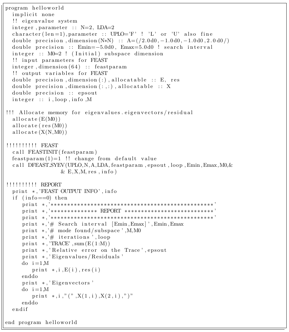
Figure 3: A very simple F90 “helloworld” example. This code can be found in <FEAST directory> /example/Hermitian/Fortran/1_dense.

To create the executable, compile and link the source program with the FEAST v3.0 library, one can use:

>ifort helloworld.f90 -o helloworld -L<FEAST directory>/lib/<arch> -lfeast_dense -lfeast -mkl
where we assume that: (i) the FORTRAN compiler is ifort the Intel’s one, (ii) the FEAST package has been installed in a directory called <FEAST directory>, (iii) the user architecture is <arch> (x64, ia64, etc.), (iv) MKL is used to link the LAPACK and BLAS libraries.

A run of the resulting executable looks like

$${\tt>./helloworld}$$

and the output of the run appears in Figure 4.

⬇

***********************************************

*********** FEAST- BEGIN **********************

***********************************************

Routine DFEAST_S{}{}

List of input parameters fpm(1:64)– if different from default

fpm(1)=1

Search interval [-5.000000000000000e+00; 5.000000000000000e+00]

Size system 2

Size subspace 2

#Linear systems 8

———————————————————————————–

#Loop | #Eig | Trace | Error-Trace | Max-Residual

———————————————————————————–

0 2 4.000000000000015e+00 1.000000000000000e+00 2.512147933894036e-15

==>FEAST has successfully converged (to desired tolerance)

***********************************************

*********** FEAST- END*************************

***********************************************

FEAST OUTPUT INFO 0

*************************************************

************** REPORT ***************************

*************************************************

# Search interval [Emin,Emax] -5.00000000000000 5.00000000000000

# mode found/subspace 2 2

# iterations 0

TRACE 4.00000000000002

Relative error on the Trace 1.00000000000000

Eigenvalues/Residuals

1 1.00000000000000 7.536443801682115E-016

2 3.00000000000001 2.512147933894036E-015

Eigenvectors

1 ( 0.707106781186547 0.707106781186549 )

2 ( 0.707106781186552 -0.707106781186545 )

Figure 4: Output results for the simple F90 “helloworld” example.

C

Similarly to the F90 example, the corresponding C source code of the helloworld example (helloworld.c) is listed in Figure 5. The executable can now be created using the gcc compiler (for example), along with the -lm library:

gcc helloworld.c -o helloworld $\backslash$
     -I<FEAST directory>/include -L<FEAST directory>/lib/<arch> -lfeast_dense -lfeast $\backslash$
     -Wl,--start-group -lmkl_intel_lp64 -lmkl_intel_thread -lmkl_core -Wl,--end-group $\backslash$
     -liomp5 -lpthread -lm
where we assume that FEAST has been compiled without runtime dependencies. In contrast, if the FEAST library was compiled using ifort alone then the flag -lifcoremt should be added above; In turn, if the FEAST library was compiled using gfortran alone, it is the flag -lgfortran that should be added instead.

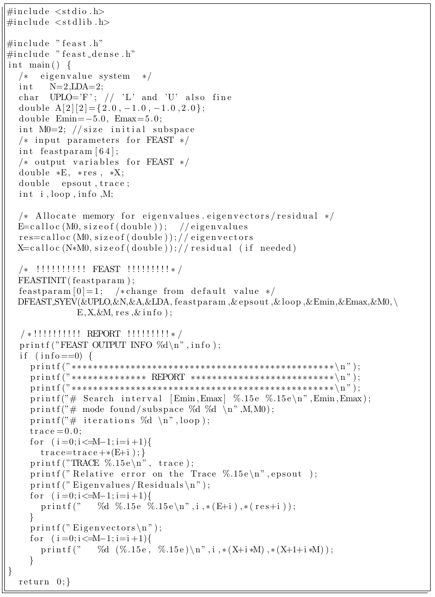
Figure 5: A very simple C “helloworld” example. This code can be found in <FEAST directory> /example/Hermitian/C/1_dense.

MPI-F90

Similarly to the F90 example, the corresponding MPI-F90 source code of the helloworld example (phelloworld.f90) is listed in Figure 6. The executable can now be created using mpif90 (for example):

mpif90 -f90=ifort phelloworld.f90 -o phelloworld $\backslash$
     -L<FEAST directory>/lib/<arch> -lpfeast_dense -lpfeast -mkl
where we assume that: (i) the Intel Fortran compiler is used, (ii) the FEAST-MPI library has been compiled using the same MPI implementation.

A run of the resulting executable looks like

$${\tt>mpirun-ppn~{}1-n<x>./phelloworld}$$

where ${\tt<x>}$ represents the number of nodes.

MPI-C

Similarly to the MPI-F90 example, the corresponding MPI-C source code of the helloworld example (phelloworld.c) is listed in Figure 6. The executable can now be created using mpicc (for example):

mpicc -cc=gcc helloworld.f90 -o helloworld $\backslash$
     -L<FEAST directory>/lib/<arch> -lpfeast_dense -lpfeast $\backslash$
     -Wl,--start-group -lmkl_intel_lp64 -lmkl_intel_thread -lmkl_core -Wl,--end-group $\backslash$
     -liomp5 -lpthread -lm
where we assume that: (i) the gnu C compiler is used, (ii) the FEAST-MPI library has been compiled using the same MPI implementation , (iii) FEAST has been compiled without runtime dependencies (otherwise see comments in C example section).

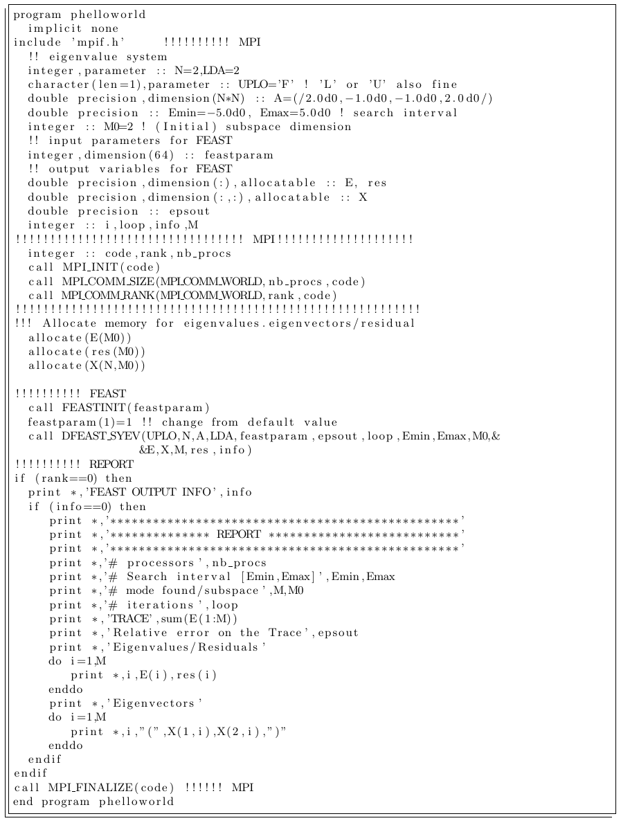
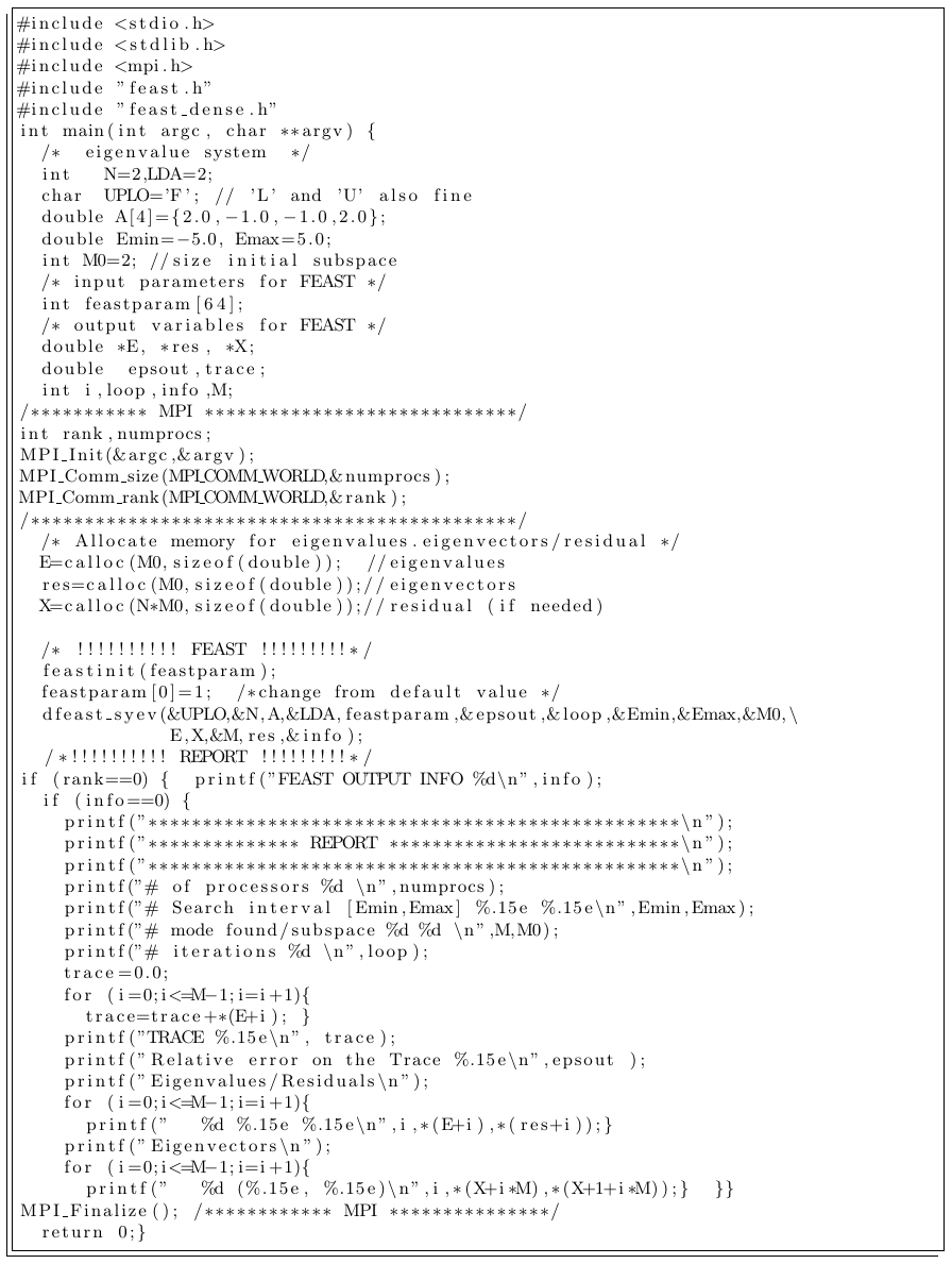
Figure 6: A very simple MPI-F90 and MPI-C “helloworld” example. These codes can be found in <FEAST directory> /example/Hermitian/<Fortran-MPI,C-MPI>/1_dense

3 FEAST Interfaces

3.1 Basics

3.1.1 Definition

There are two different type of interfaces available in the FEAST library:

Reverse communication interfaces (RCI): $${\tt{\bf\large T}feast\_{\bf\large Y}rci}$$ with their expert version $${\tt{\bf\large T}feast\_{\bf\large Y}rcix}$$ These interfaces constitute the kernel of FEAST. They are matrix free format (the interfaces are independent of the matrix data formats), users can then define their own explicit or implicit data format. Mat-vec routines and direct/iterative linear system solvers must also be provided by the users. Format predefined interfaces: $${\tt{\bf T}feast\_{\bf\large YF}ev}\quad\mbox{ and }\quad{\tt{\bf\large T}feast\_{\bf\large YF}gv},$$ with their expert versions $${\tt{\bf T}feast\_{\bf\large YF}evx}\quad\mbox{ and }\quad{\tt{\bf\large T}feast\_{\bf\large YF}gvx},$$ These interfaces for standard “ev” and generalized “gv” problems can be considered as predefined optimized drivers for Tfeast_Yrci and Tfeast_Yrcix that act on commonly used matrix data storage (dense, banded and sparse-CSR), using predefined mat-vec routines and preselected inner linear system solvers.

• T is the data type of matrix A (and matrix B if any) i.e. Value of T Type of matrices s single precision d double precision c complex single precision z complex double precision

• YF is the problem type (Symmetric, Hermitian, or General) and storage format (Dense, Banded, Sparse). Together they define the problem.

  Y	F	Problem Type	Matrix Format	Linear Solver
  s	y	Symmetric	Dense	LAPACK
  h	e	Hermitian	Dense	LAPACK
  g	e	General	Dense	LAPACK
  s	b	Symmetric	Banded	SPIKE
  h	b	Hermitian	Banded	SPIKE
  g	b	General	Banded	SPIKE
  s	csr	Symmetric	Sparse	MKL-PARDISO
  h	csr	Hermitian	Sparse	MKL-PARDISO
  g	csr	General	Sparse	MKL-PARDISO

The different FEAST interface names and combinations are summarized in Table 2.

RCI- interfaces
{s,d,c,z}feast_srci
{c,z}feast_hrci
{s,d,c,z}feast_grci
DENSE- interfaces
{s,d,c,z}feast_sy{ev,gv}
{c,z}feast_he{ev,gv}
{s,d,c,z}feast_ge{ev,gv}

BANDED- interfaces
{s,d,c,z}feast_sb{ev,gv}
{c,z}feast_hb{ev,gv}
{s,d,c,z}feast_gb{ev,gv}
SPARSE- interfaces
{s,d,c,z}feast_scsr{ev,gv}
{c,z}feast_hcsr{ev,gv}
{s,d,c,z}feast_gcsr{ev,gv}

Table 2: List of all FEAST interfaces available in FEAST v3.0. Expert routines include x at the end.

3.1.2 Common Declarations

The arguments list for the FEAST interfaces are commonly defined as follows:

Tfeast_Y{interface}  ({List},fpm,epsout,loop,{List-I},M0,E,X,M,res,info)
Tfeast_Y{interface}x ({List},fpm,epsout,loop,{List-I},M0,E,X,M,res,info,Zne,Wne)

where {List} and {List-I} denote a series of arguments that are specific to each interfaces and will be presented in the next sections. The rest of the arguments are common to both RCI and predefined FEAST interfaces and their definition is given in Table 3.

	Type (Fortran)	Input/Output	Description
fpm	integer(64)	in	FEAST input parameters (see Table 9)
			The size should be at least 64
epsout	Type(S) if T=s,c	out	Relative error on the trace
	or		$|{\tt trace}_{k}-{\tt trace}_{k-1}|/\max({\tt|Emin|,|Emax|})$, or
	Type(D) if T=d,z		$|{\tt trace}_{k}-{\tt trace}_{k-1}|/({\tt|Emid|+r})$
loop	integer	out	# of FEAST subspace iterations
M0	integer	in/out	Search subspace dimension
			On entry: initial guess (M0>M)
			On exit: new suitable M0 if guess too large
E	Type(S)(M0) if TY=ss,ch	out	Eigenvalues
	Type(D)(M0) if TY=ds,zh		the first M values are in the search interval
	Type(C)(M0) if TY=sg,cg,cs		the others M0-M values are outside
	Type(Z)(M0) if TY=dg,zg,zs
X	Type(S)(N,M0) if TY=ss	in/out	Eigenvectors (N: size of the system)
	Type(D)(N,M0) if TY=ds		On entry: guess subspace if fpm(5)=1
	Type(C)(N,M0) if TY=ch,cs		On exit: (right) eigenvectors solutions X(1:N,1:M)
	Type(Z)(N,M0) if TY=zh,zs		(same ordering as in E)
	Type(C)(N,2*M0) if TY=sg,cg		Remark: * left vectors (if calculated) in X(1:N,M0+1:M0+M)
	Type(Z)(N,2*M0) if TY=dg,zg		* if fpm(14)=1, first $\bf Q$ subspace on exit
M	integer	out	# Eigenvalues found in search interval
			# estimated eigenvalues if fpm(14)=2
res	Type(S)(M0) if TY=ss,ch,cs	out	Relative residual res(1:M) (right); res(M0+1:M0+M) (left)
	Type(D)(M0) if TY=ds,zh,zs		(right) $\bf||Ax_{i}-\lambda_{i}Bx_{i}||_{1}/||\alpha Bx_{i}||_{1}$
	Type(S)(2*M0) if TY=sg,cg		(left) $\bf||A^{H}x_{i}-\lambda_{i}^{*}B^{H}x_{i}||_{1}/||\alpha B^{H}x_{i}||_{1}$
	Type(D)(2*M0) if TY=dg,zg		Remark: * ${\tt\alpha}=\max({\tt|Emin|,|Emax|})$ or ${\tt\alpha}=({\tt|Emid|+r})$
			* if fpm(14)=2, res(1:M) running average for M
info	integer	out	Error handling (if =0: successful exit)
			(see Table 10 for all INFO return codes)
Zne,Wne	Type(C)(fpm(2)) if TY=ss,ch	in	Custom integration nodes and weights- Expert mode
	Type(Z)(fpm(2)) if TY=ds,zh
	Type(C)(fpm(8)) if TY=sg,cg,cs
	Type(Z)(fpm(8)) if TY=dg,zg,zs

Table 3: List of arguments common for the RCI and predefined FEAST interfaces.
Remark: the arrays E, X and res return the eigenpairs and associated residuals. The solutions within the intervals are contained in the first M components of the arrays. The left vectors (if calculated) are contained in X(1:N,M0+1:M0+M). Note for expert use: the solutions that are directly outside the intervals can also be found with less accuracy in the other M0-M components (i.e. from element M+1 to M0). In addition where spurious solutions may be found in the processing of the FEAST algorithm, those are put at the end of the arrays E and X and are flagged with the value $-1$ in the array res.

3.2 FEAST_RCI interfaces

These interfaces are useful if your application requires specific linear system solvers (direct or iterative) or/and specific matrix storage (explicit or implicit). If this is not the case, you may want to skip this section and go directly to the section 3.3 on predefined interfaces.

3.2.1 Specific declarations

The arguments list for the FEAST_RCI interfaces is defined as follows:

Tfeast_Yrci ({List-rci},fpm,epsout,loop,{List-I},M0,E,X,M,res,info)

Tfeast_Yrcix ({List-rci},fpm,epsout,loop,{List-I},M0,E,X,M,res,info,Zne,Wne)

The series of arguments in {List-rci} and {List-I} are defined in Table 4 and their description is provided in Table 5.

T	Y	List-rci	List-I
d,s	s	{ijob,N,Ze,work1,zwork2,Aq,Bq}	{Emin,Emax}
z,c	h	{ijob,N,Ze,zwork1,zwork2,zAq,zBq}	{Emin,Emax}
d,s	g	{ijob,N,Ze,zwork1,zwork2,zAq,zBq}	{Emid,r}
z,c	s	{ijob,N,Ze,zwork1,zwork2,zAq,zBq}	{Emid,r}
z,c	g	{ijob,N,Ze,zwork1,zwork2,zAq,zBq}	{Emid,r}

Table 4: List of arguments specific for the Tfeast_Yrci{x} interfaces.

	Type (Fortran)	Input/	Description
		Output
ijob	integer	in/out	ID of the FEAST_RCI operation
			On entry: ijob=-1 (initialization)
			On exit: ijob=0,10,11,20,21,30,31,40,41
N	integer	in	Size of the system
Ze	Type(C) if T=s,c	out	Coordinate along the complex contour
	Type(Z) if T=d,z
work1	Type(S)(N,M0) if T=s	in/out	Workspace
	Type(D)(N,M0) if T=d
zwork1	Type(C)(N,M0) if TY=ch,cs	in/out	Workspace
	Type(C)(N,2*M0) if TY=sg,cg
	Type(Z)(N,M0) if TY=zh,zs
	Type(Z)(N,2*M0) if TY=dg,zg
zwork2	Type(C)N,M0) if T=s,c	in/out	Workspace
	Type(Z)(N,M0) if T=d,z
Aq or Bq	Type(S)(M0,M0) if T=s	in/out	Workspace for the reduced eigenvalue problem
	Type(D)(M0,M0) if T=d
zAq or zBq	Type(C)(M0,M0) if T=s,c	in/out	Workspace for the reduced eigenvalue problem
	Type(Z)(M0,M0) if T=d,z
Emin	Type(S) if T=s,c	in	Lower bound of search interval
	Type(D) if T=d,z		Hermitian problem
Emax	Type(S) if T=s,c	in	Upper bound of search interval
	Type(D) if T=d,z		Hermitian problem
Emid	Type(C) if T=s,c	in	Coordinate center of the contour ellipse
	Type(Z) if T=d,z		non-Hermitian problem
r	Type(S) if T=d,z	in	Horizontal radius of the contour ellipse
	Type(D) if T=s,c		non-Hermitian problem

Table 5: Definition of arguments specific for the Tfeast_Yrci{x} interfaces.

3.2.2 RCI Mechanism

Using the FEAST_RCI interfaces, the ijob parameter must first be initialized with the value $-1$. Once the RCI interface is called, the value of the ijob output parameter, if different than $0$, is used to identify the FEAST operation that needs to be done by the user Users have then the possibility to customize their own matrix direct or iterative factorization and linear solve techniques as well as their own matrix multiplication routine. Table 6 lists all the required cases options needed using Tfeast_Yrci{X} interfaces, depending on the choices for TY. The general reverse communication interface (RCI) mechanism is detailed in Figure 7.

T	Y	ijob parameter values - cases required
d,s	s	{10,11,30,40}
z,c	h	{10,11,{20},21,30,40}
d,s	g	{10,11,{20},21,30,31,40,41}
z,c	s	{10,11,{20},21,30,31,40,41}
z,c	g	{10,11,{20},21,30,31,40,41}

Table 6: Required options for the Tfeast_Yrci{x} interfaces.

⬇

ijob=-1 ! initialization

do while (ijob/=0)

call Tfeast_Yrci{x}({List-rci},fpm,epsout,loop,{List-I},M0,E,X,M,res,info,{Zne,Wne})

select case(ijob)

case(10) !!Factorize the complex matrix Az <=(ZeB-A) - or factorize a preconditioner of Az

……………. <<< user entry

case(11) !!Solve the linear system with fpm(23) rhs; Az * Qz=zwork2(1:N,1:fpm(23))

!!Result in zwork2 <= Qz(1:N,1:fpm(23))

……………. <<< user entry

case(20) !!Factorize (*only if* needed by case(21)) the complex matrix Az’<=Az^H

!!ATTENTION: The matrix Az from case(10) cannot be overwritten

!! - this option would require additional memory storage-

!!REMARK: case(20) becomes obsolete if the solve in case(21) can be performed

!! by reusing the factorization in case(10)

……………. <<< user entry

case(21) !!Solve the linear system with fpm(23) rhs; Az^H * Qz=zwork2(1:N,1:fpm(23))

!!Result in zwork2 <= Qz(1:N,1:fpm(23))

……………. <<< user entry

case(30) !!Perform multiplication A * X(1:N,i:j) result in {z}work1(1:N,i:j)

!! where i=fpm(24) and j=fpm(24)+fpm(25)-1

……………. <<< user entry

case(31) !!Perform multiplication A^H * X(1:N,i:j) result in {z}work1(1:N,i:j)

!! where i=fpm(34) and j=fpm(34)+fpm(35)-1

……………. <<< user entry

case(40) !!Perform multiplication B * X(1:N,i:j) result in {z}work1(1:N,i:j)

!! where i=fpm(24) and j=fpm(24)+fpm(25)-1

……………. <<< user entry

case(41) !!Perform multiplication B^H * X(1:N,i:j) result in {z}work1(1:N,i:j)

!! where i=fpm(34) and j=fpm(34)+fpm(35)-1

……………. <<< user entry

end select

end do

Figure 7: Description of the general FEAST reverse communication interface mechanism (Fortran example).
Remark: (i) For standard eigenvalue problems case(40) and case(41) involve only copy operations; (ii) If the whole interface is called within an MPI-environment and the code is linked to FEAST_MPI (i.e. -lpfeast), the operations on the contour integration and the mat-vec operations with multiple rhs, will be automatically distributed among the MPI processes.

3.3 FEAST predefined interfaces

3.3.1 Specific declarations

For the generalized eigenvalue problem:

Tfeast_YFgv  ({List-A},{List-B},fpm,epsout,loop,{List-I},M0,E,X,M,res,info)
Tfeast_YFgvx ({List-A},{List-B},fpm,epsout,loop,{List-I},M0,E,X,M,res,info,Zne,Wne)

For the standard eigenvalue problem:

Tfeast_YFev  ({List-A},fpm,epsout,loop,{List-I},M0,E,X,M,res,info)
Tfeast_YFevx ({List-A},fpm,epsout,loop,{List-I},M0,E,X,M,res,info,Zne,Wne)

where the series of arguments in each {List-A}, {List-B}, and {List-I}, are specific to the values of T, Y and F, and are given in Table 7. The definition of the arguments in {List-A} and {List-B} is given in Table 8. The definitions for the dense, banded and CSR matrix data structures are also provided in the next section.

T	Y	F	List-A	List-B	List-I
Dense
z,c	s	y	{ UPLO, N, A, LDA }	{ B, LDB }	{ Emid, r }
z,c	h	e	{ UPLO, N, A, LDA }	{ B, LDB }	{ Emin, Emax }
z,c	g	e	{ N, A, LDA }	{ B, LDB }	{ Emid, r }
d,s	s	y	{ UPLO, N, A, LDA }	{ B, LDB }	{ Emin, Emax }
d,s	g	e	{ N, A, LDA }	{ B, LDB }	{ Emid, r }
Banded
z,c	s	b	{ UPLO, N, kla, A, LDA }	{ klb, B, LDB }	{ Emid, r }
z,c	h	b	{ UPLO, N, kla, A, LDA }	{ klb, B, LDB }	{ Emin, Emax }
z,c	g	b	{ N, kla, kua, A, LDA }	{ klb, kub, B, LDB }	{ Emid, r }
d,s	s	b	{ UPLO, N, kla, A, LDA }	{ klb, B, LDB }	{ Emin, Emax }
d,s	g	b	{ N, kla, A, LDA }	{ klb, kub, B, LDB }	{ Emid, r }
Sparse
z,c	s	csr	{ UPLO, N, A, IA, JA }	{ B, IB, JB }	{ Emid, r }
z,c	h	csr	{ UPLO, N, A, IA, JA }	{ B, IB, JB }	{ Emin, Emax }
z,c	g	csr	{ N, A, IA, JA }	{ B, IB, JB }	{ Emid, r }
d,s	s	csr	{ UPLO, N, A, IA, JA }	{ B, IB, JB }	{ Emin, Emax }
d,s	g	csr	{ N, A, IA, JA }	{ B, IB, JB }	{ Emid, r }

Table 7: List of arguments specific for the Tfeast_YF{ev,gv}{x} interfaces.

	Type (Fortran)	Input/	Description
		Output
UPLO	character(len=1)	in	Matrix Storage (’F’,’L’,’U’)
			’F’: Full; ’L’: Lower; ’U’: Upper
N	integer	in	Size of the system
kla	integer	in	The number of subdiagonals
			within the band of A.
klu	integer	in	The number of superdiagonals
			within the band of A.
klb	integer	in	The number of subdiagonals
			within the band of B.
kub	integer	in	The number of superdiagonals
			within the band of B.
A	Same type as T	in	Eigenvalue system (Stiffness) matrix
	with 2D dimension: (LDA,N) if Dense
	with 2D dimension: (LDA,N) if Banded
	with 1D dimension: (IA(N+1)-1) if Sparse
B	Same type as T	in	Eigenvalue system (Mass) matrix
	with 2D dimension: (LDB,N) if Dense
	with 2D dimension: (LDB,N) if Banded
	with 1D dimension: (IB(N+1)-1) if Sparse
LDA	integer	in	Leading dimension of A;
			LDA>=N if Dense
			LDA>=2kla+1 if Banded; UPLO=’F’
			LDA>=kla+1 if Banded; UPLO/=’F’
LDB	integer	in	Leading dimension of B;
			LDB>=N if Dense
			LDB>=2klb+1 if Banded; UPLO=’F’
			LDB>=klb+1 if Banded; UPLO/=’F’
IA	integer(N+1)	in	Sparse CSR Row array of A.
JA	integer(IA(N+1)-1)	in	Sparse CSR Column array of A.
IB	integer(N+1)	in	Sparse CSR Row array of B.
JB	integer(IB(N+1)-1)	in	Sparse CSR Column array of B.

Table 8: Definition of arguments specific for the Tfeast_YF{ev,gv}{x} interfaces.

3.3.2 Matrix storage

Let us consider a standard eigenvalue problem and the following (stiffness) matrix A:

$${\bf A}=\begin{pmatrix}a_{11}&a_{12}&0&0\\ a_{21}&a_{22}&a_{23}&0\\ 0&a_{32}&a_{33}&a_{34}\\ 0&0&a_{43}&a_{44}\\ \end{pmatrix}$$ (2)

where $a_{ij}=a_{ji}^{*}$ for $i\neq j$ (i.e. $a_{ij}=a_{ji}$ if the matrix is real). Using the FEAST predefined interfaces, this matrix could be stored in dense, banded or sparse format as follows:

• Using the dense format, A is stored in a two dimensional array in a straightforward fashion. Using the options UPLO=’L’ or UPLO=’U’, the lower triangular and upper triangular part respectively, do not need to be referenced.

• Using the banded format, A is also stored in a two dimensional array following the banded LAPACK-type storage:
  

  $${\bf A=}\begin{pmatrix}*&a_{12}&a_{23}&a_{34}\\ a_{11}&a_{22}&a_{33}&a_{44}\\ a_{21}&a_{32}&a_{43}&*\end{pmatrix}$$

  
  

  In contrast to LAPACK, no extra-storage space is necessary since LDA>=2*kla+1 if UPLO=’F’ (LAPACK banded storage would require LDA>=3*kla+1). For this example, the number of subdiagonals or superdiagonals is kla=1. Using the option UPLO=’L’ or UPLO=’U’, the kla rows respectively above or below the diagonal elements row, do not need to be referenced (or stored).

• Using the sparse storage, the non-zero elements of A are stored using a set of one dimensional arrays (A,IA,JA) following the definition of the CSR (Compressed Sparse Row) format

  $$\begin{array}[]{rl}{\bf A=}&(a_{11},a_{12},a_{21},a_{22},a_{23},a_{32},a_{33},a_{34},a_{43},a_{44})\\ {\bf IA=}&(1,3,6,9,11)\\ {\bf JA=}&(1,2,1,2,3,2,3,4,3,4)\end{array}$$

  Using the option UPLO=’L’ or UPLO=’U’, one would get respectively

  $$\begin{array}[]{rl}{\bf A=}&(a_{11},a_{21},a_{22},a_{32},a_{33},a_{43},a_{44})\\ {\bf IA=}&(1,2,4,6,8)\\ {\bf JA=}&(1,1,2,2,3,3,4)\end{array}\mbox{~{}~{}~{}~{}and~{}~{}~{}~{}}\hfill\begin{array}[]{rl}{\bf A=}&(a_{11},a_{12},a_{22},a_{23},a_{33},a_{34},a_{44})\\ {\bf IA=}&(1,3,5,7,8)\\ {\bf JA=}&(1,2,2,3,3,4,4)\end{array}$$

Finally, the (mass) matrix B that appears in generalized eigenvalue systems, should use the same family of storage format than the matrix A. It should be noted, however, that the bandwidth can be different for the banded format (klb can be different than kla), and the position of the non-zero elements can also be different for the sparse format (CSR coordinates IB,JB can be different than IA,JA).

4 FEAST Parameters and Search Contour

4.1 Input FEAST parameters

In the common argument list, the input parameters for the FEAST algorithm are contained into an integer array of size 64 named here fpm. Prior calling the FEAST interfaces, this array needs to be initialized using the routine feastinit as follows (Fortran notation):

call feastinit(fpm)

All input FEAST parameters are then set to their default values. The detailed list of these parameters is given in Table 9.

fpm(i) Fortran	Description	Default value
fpm[i-1] C
i=1	Print runtime comments on screen (0: No; 1: Yes)	0
i=2	# of contour points for Hermitian FEAST (half-contour)	8
	if fpm(16)=0,2, values permitted (1 to 20, 24, 32, 40, 48, 56)
	if fpm(16)=1, all values permitted
i=3	Stopping convergence criteria for double precision ($\epsilon=10^{\tt-fpm(3)}$)	12
i=4	Maximum number of FEAST refinement loop allowed ($\geq 0$)	20
i=5	Provide initial guess subspace (0: No; 1: Yes)	0
i=6	Convergence criteria (for the eigenpairs in the search interval)	1
	0: Using relative error on the trace epsout i.e. epsout$<\epsilon$
	1: Using relative residual res i.e. $\max_{i}{\tt res(i)}<\epsilon$
i=7	Stopping convergence criteria for single precision ($\epsilon=10^{\tt-fpm(7)}$)	5
i=8	# of contour points for non-Hermitian FEAST (full-contour)	16
	if fpm(17)=0, values permitted (2 to 40, 48, 64, 80, 96, 112)
	if fpm(17)=1, all values permitted ($>$2)
i=9	User defined MPI communicator for a given search interval	MPI_COMM_WORLD
i=10	Store factorizations with the predefined interfaces (0: No; 1: Yes).	0
i=14	1: FEAST normal execution; 1: Return subspace Q after 1 contour;	0
	2: Estimate #eigenvalues inside search interval
i=16	Integration type for Hermitian (0: Gauss; 1: Trapezoidal; 2: Zolotarev)	0
i=17	Integration type for non-Hermitian (0: Gauss, 1: Trapezoidal)	1
i=18	Ellipse contour ratio - fpm(18)/100 = ratio ’vertical axis’/’horizontal axis’	100
i=19	Rotation angle in degree [-180:180] for ellipse using non-Hermitian FEAST	0
	Origin of the rotation is the vertical axis.
i=40-63	unused
All Others	Reserved value	N/A

Table 9: List of input FEAST parameters and default values obtained with the routine feastinit.
Remark: Using the C language, the components of the fpm array starts at 0 and stops at 63. Therefore, the components fpm[j] in C (j=0-63) must correspond to the components fpm(i) in Fortran (i=1-64) specified above (i.e. fpm[i-1]=fpm(i)).

4.2 Defining a search contour

Figure 8 summarizes the different search contour options possible for both the Hermitian and non-Hermitian FEAST algorithms.

For the Hermitian case, the user must then specify a 1-dimensional real-valued search interval $[E_{min},E_{max}]$. These two points are used to define a circular or ellipsoid contour $\cal C$ centered on the real axis, and along which the complex integration nodes are generated. The choice of a particular quadrature rule will lead to a different set of relative positions for the nodes and associated quadrature weights. Since the eigenvalues are real, it is convenient to select a symmetric contour with the real axis (${\cal C}={\cal C}^{*}$) since it only requires to operate the quadrature on the half-contour (e.g. upper half).

With a non-Hermitian problem, it is necessary to specify a 2-dimensional search interval that surrounds the wanted complex eigenvalues. Circular or ellipsoid contours can also be used and they can be generated using standard options included into FEAST v3.0. These are defined by a complex midpoint $E_{mid}$ and a radius $r$ for a circle (for an ellipse the ratio between the horizontal axis $2r$ and vertical axis can also be specified, as well as an angle of rotation). in some applications where the eigenvalues of interest belong to a particular subset in the complex plane, A “Custom Contour” feature is also supported in FEAST v3.0 that allows to account for arbitrary quadrature nodes and weights.

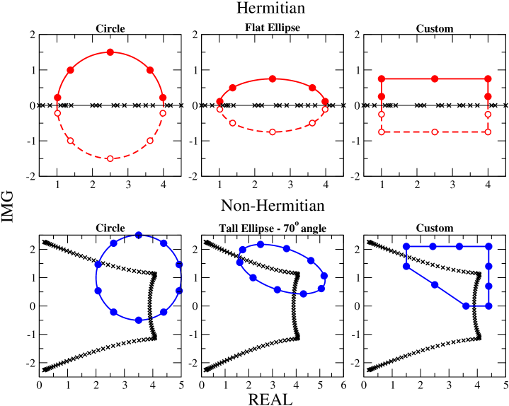
Figure 8: Various search contour examples for the Hermitian and the non-Hermitian FEAST algorithms. Both algorithms feature standard ellipsoid contour options and the possibility to define custom arbitrary shapes. In the Hermitian case, the contour is symmetric with the real axis and only the nodes in the upper-half may be generated. In the non-Hermitian case, a full contour is needed to enclose the wanted complex eigenvalues. Some data used to generate these plots:
Hermitian case: fpm(2)=5 for all, $[E_{min},E_{max}]=[1,4]$, $r=1.5$ for all; fpm(18)=50 for the flat ellipse; expert routine for the custom contour
Non-Hermitian case: fpm(8)=10 for all; $E_{mid}=3.5+i$ and $r=1.5$ for circle; $E_{mid}=3.4+1.3i$, $r=0.75$, fpm(18)=200, fpm(19)=70 for tall rotated ellipse; expert routine for the custom contour

4.3 Output FEAST info details

Errors and warnings encountered during a run of the FEAST package are stored in an integer variable, info. If the value of the output info parameter is different than “0”, either an error or warning was encountered. The possible return values for the info parameter along with the error code descriptions, are given in Table 10.

info	Classification	Description
$202$	Error	Problem with size of the system N
$201$	Error	Problem with size of subspace M0
$200$	Error	Problem with Emin,Emax or Emid, r
$(100+i)$	Error	Problem with $i^{th}$ value of the input FEAST parameter (i.e fpm(i))
$6$	Warning	FEAST converges but subspace is not bi-orthonormal
$5$	Warning	Only stochastic estimation of #eigenvalues returned fpm(14)=2
$4$	Warning	Only the subspace has been returned using fpm(14)=1
$3$	Warning	Size of the subspace M0 is too small (M0<=M)
$2$	Warning	No Convergence (#iteration loops$>$fpm(4))
$1$	Warning	No Eigenvalue found in the search interval
$0$	Successful exit
$-1$	Error	Internal error for allocation memory
$-2$	Error	Internal error of the inner system solver in FEAST predefined interfaces
$-3$	Error	Internal error of the reduced eigenvalue solver
		Possible cause for Hermitian problem: matrix B may not be positive definite
$-(100+i)$	Error	Problem with the $i^{th}$ argument of the FEAST interface

Table 10: Return code descriptions for the parameter info.
Remark: In some extreme cases the return value info=1 may indicate that FEAST has failed to find the eigenvalues in the search interval. This situation would appear only if a very large search interval is used to locate a small and isolated cluster of eigenvalues (i.e. in case the dimension of the search interval is many orders of magnitude off-scaling). For this case, it is then either recommended to increase the number of contour points fpm(2) or simply rescale more appropriately the search interval.

5 FEAST: General use

This section briefly presents to the FEAST users a list of specifications (i.e. what is needed from users), expectations (i.e. what users should expect from FEAST), and directions for achieving performances (i.e. including parallel scalability and current limitations).

5.1 Single search interval and FEAST-SMP

Specifications:

• the search interval and the size of the subspace $\rm M_{0}$ (overestimation of the number of eigenvalues $\rm M$ within); If needed, once a search interval is defined, the user can take advantage of fast stochastic estimates for $\rm M$ presented in Section 7.1 (tools for FEAST).

• the system matrix in dense, banded or sparse-CSR format if FEAST predefined interfaces are used, or a high-performance complex direct or iterative system solver and matrix-vector multiplication routine if FEAST RCI interfaces are used instead.

Expectations:

• robust and systematic convergence to very high accuracy seeking up to $1000$’s eigenpairs (no known failed case for the Hermitian problem);

• the convergence rate depends on a trade-off between the choice of the search subspace size $\rm M0$ and the number of contour points (and nature of the quadrature). For most applications FEAST Hermitian will convergence to machine precision in 3 iterations, using a Gauss-Legendre quadrature with ${\rm M_{0}\geq 1.5M}$ and ${\tt fpm(2)=8}$. If the convergence is too slow, you can: (i) keep on increasing $\rm M_{0}$ or/and fpm(2) (fpm(8) for non-Hermitian) for the Gauss-Legendre or Trapezoidal quadrature; (ii) decrease the ellipse ratio fpm(18) for the Hermitian problem; (iii) choose a more robust approach consisting of using the Zolotarev quadrature for the Hermitian problem with fpm(16)=2 (the subspace does not need to be large $\rm M_{0}\sim M$).

Directions for achieving performances:

• $\rm M_{0}$ should be much smaller than the size of the eigenvalue problem, then the arithmetic complexity should mainly depend on the inner system solver (i.e. $\rm O(NM_{0})$ for narrow banded or sparse system);

• storing the factorizations with option fpm(10)=1 for the predefined interfaces, will significantly improve the performances (for FEAST DENSE in particular), but can significantly increase the memory usage ($\sim\times$fpm(2) or fpm(8) for non-Hermitian);

• parallel scalability performances at the third level of parallelism depends on the shared memory capabilities of the inner system solver i.e. via the shell variable MKL_NUM_THREADS if a Intel-MKL solver is used (LAPACK or MKL-PARDISO) or the the shell variable OMP_NUM_THREADS if SPIKE-SMP is used for the banded interfaces;

• if $\rm M_{0}$ increases significantly for a given search interval, the complexity $\rm O(M_{0}^{3})$ for solving the reduced system could become significant (typically, if $\rm M_{0}>2000$). In this case it is recommended to consider multiple search intervals to be solved in parallel. For example, if $10^{4}$ eigenpairs of a very large system are needed, many search intervals could be used simultaneously to decrease the size of the reduced dense generalized eigenproblem (e.g. if $10$ intervals are selected the size of each reduced problem would then be $\sim 10^{3}$);

• For very large general sparse and challenging systems, it is strongly recommended for expert application users to make use of FEAST-RCI with customized highly-efficient system solvers such as: domain decompositions, or iterative solvers with/without preconditioners;

5.2 Single search interval and FEAST-MPI

Specifications:

• Same general specification than for the FEAST-SMP;

• MPI environment application code and link to the FEAST-MPI library.

Expectations:

• same general expectation than for FEAST-SMP;

• ideally, linear scalability performances with the number of MPI processes up to the number of linear systems (i.e. Factorization stage) $N_{e}$ to perform by contour. If the number of MPI processes is exactly (optimally) equal to $N_{e}$ which is equal to either fpm(2) for FEAST Hermitian or fpm(8) for FEAST non-Hermitian, the factorization of the system matrices is kept in memory along the FEAST iterations and “superlinear scalability” can then be expected. We note one particular case: if the system matrix is real non-symmetric with Img{Emid}=0, and with fpm(8) even number, the number of factorizations becomes fpm(8)/2.

Directions for achieving performances:

• same general directions than for FEAST-SMP;

• for a given search interval, the second and third level of parallelism is then easily achieved by MPI (along the contour points) calling OpenMP (i.e shared memory linear system solver). Among the two levels of parallelism offered here, there is a trade-off between the choice of the number of MPI processes and threads by MPI process. For example let us consider: (i) the use of FEAST-SPARSE interface, (ii) $8$ contour points (i.e. $8$ linear systems to solve), and (iii) a cluster of $4$ physical nodes with $8$ cores/threads by nodes; the two following options (among many others) should be considered to run the MPI code myprog:

  $${\tt>mpirun-genv~{}MKL\_NUM\_THREADS~{}8-ppn~{}1-n~{}4~{}./myprog}$$

  where $8$ threads can be used on each node, and where each physical node ends up solving consecutively two linear systems using $8$ threads. This option saves memory.

  $${\tt>mpirun-genv~{}MKL\_NUM\_THREADS~{}4-ppn~{}2-n~{}8~{}./myprog}$$

  where $4$ threads can be used on each node, and where the MPI processes end up solving simultaneously the $8$ linear systems using $4$ threads. This option should provide better performance but it is more demanding in memory (two linear systems are stored on each node).

  In contrast if $8$ physical nodes are available, the best possible option for $8$ contour points becomes:

  $${\tt>mpirun-genv~{}MKL\_NUM\_THREADS~{}8-ppn~{}1-n~{}8~{}./myprog}$$

  where all the $64$ cores are then used.

• If more physical nodes than contour points are available, scalability cannot be achieved at the second level parallelism anymore, but multiple search intervals could then be considered (i.e. first level of parallelism).

5.3 Multiple search intervals and FEAST-MPI

Specifications:

• same general specification than for the FEAST-MPI using a single search interval;

• a new flag fpm(9) can easily by defined by the user to set up a local MPI communicator associated to different cluster of nodes for each search interval (which is set to MPI_COMM_WORLD by default). An example on how one can proceed for two search intervals is given in Figure 9. This can easily be generalized to any numbers of search intervals.

Expectations:

• same general expectation than for FEAST-MPI using a single search interval;

• perfect parallelism using multiple neighboring search intervals without overlap (overall orthogonality should also be preserved).

Directions for achieving performances:

• same general directions than for FEAST-MPI using a single search interval;

• in practical applications, the users should have a good apriori estimates of the distribution of the overall eigenvalue spectrum in order to make an efficient use of the first level of parallelism (i.e. in order to specified the search intervals). Users can currently take advantage of fast stochastic estimates presented in Section 7.1. Future developments of FEAST will include runtime automatic strategies to partition the search intervals.

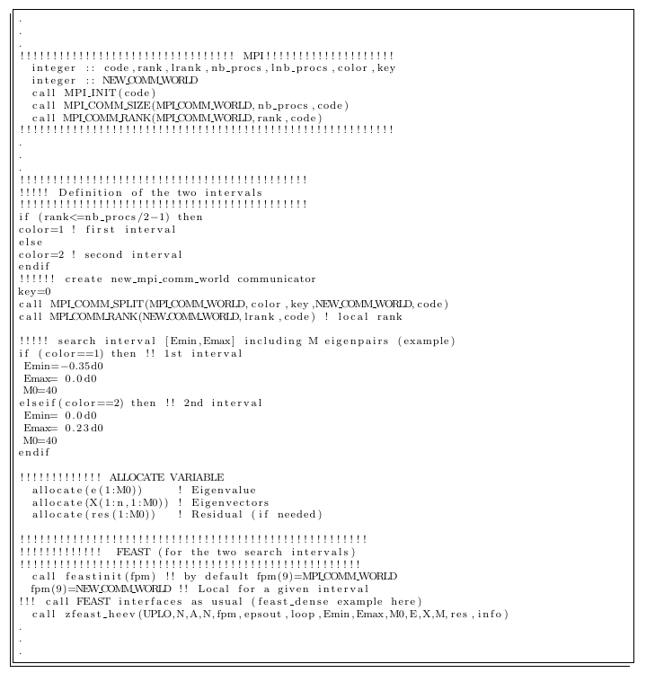
Figure 9: A simple MPI-F90 example procedure using two search intervals and the flag fpm(9). In this example, if the code is executed using n MPI-processes, the first search interval would be using n/2 processes while n-n/2 will be used by the second search interval. Driver examples that include three levels of parallelism can be found in all subdirectories of <FEAST directory> /example/Fortran-MPI/ and <FEAST directory> /example/C-MPI/ (see FEAST application section for more details).

6 FEAST in action

6.1 Examples: Hermitian/Non-Hermitian; Fortran/C/MPI; Dense/Banded/Sparse

The $FEASTROOT/example directory provides Fortran, Fortran-MPI, C and MPI-C examples for using the FEAST predefined interfaces. The Fortran examples are written in F90 but it should be straightforward for the user to transform then into F77 if needed (since FEAST uses F77 argument-type interfaces). Examples include four particular types of eigenvalue problems:

Example 1

a “real symmetric” generalized eigenvalue problem $\bf Ax=\lambda Bx$ , where $\bf A$ is real symmetric and $\bf B$ is symmetric positive definite. $\bf A$ and $\bf B$ are of the size $\rm N=1671$ and have the same sparsity pattern with number of non-zero elements $\rm NNZ=11435$.

Example 2

a “complex Hermitian” standard eigenvalue problem $\bf Ax=\lambda x$, where $\bf A$ is complex Hermitian. $\bf A$ is of size $\rm N=600$ with number of non-zero elements $\rm NNZ=2988$.

Example 3

a “real non-symmetric” generalized eigenvalue problem $\bf Ax=\lambda Bx$ , where $\bf A$ and $\bf B$ are considered real non-symmetric. $\bf A$ and $\bf B$ are of the size $\rm N=1671$ and have the same sparsity pattern with number of non-zero elements $\rm NNZ=13011$.

Example 4

a “complex symmetric” standard eigenvalue problem $\bf Ax=\lambda x$, where $\bf A$ is complex symmetric. $\bf A$ is of size $\rm N=801$ with number of non-zero elements $\rm NNZ=24591$.

Examples are solved in double precision arithmetic (Example 1 and 2 also include single precision drivers) and either a dense, banded or sparse storage for the matrices.

The $FEASTROOT/example/{Hermitian,non-Hermitian} directories contain the subdirectories Fortran, C, Fortran-MPI, C-MPI which, in turn, contain similar subdirectories 1_dense, 2_banded, 3_sparse with source code drivers for the above four examples in single and double precisions.

In order to compile and run the examples of the FEAST package, please follow the following steps:

1. Go to the directory $FEASTROOT/example

2. Edit the make.inc file and follow the directions to customize appropriately: (i) the name/path of your F90, C and MPI compilers (if you wish to compile and run the F90 examples alone, it is not necessary to specify the C compiler as well as MPI and vice-versa); (ii) the path LOCLIBS for the FEAST libraries and both paths and names in LIBS of the MKL-PARDISO, LAPACK and BLAS libraries (if you do not wish to compile the sparse examples there is no need to specify the path and name of the MKL-PARDISO library).

   By default, all the options in the make.inc assumes calling the FEAST library compiled with no-runtime dependency (add the appropriate flags -lifcoremt, -lgfortran, etc. otherwise). Additionally, LIBS in make.inc uses by default the Intel-MKL (v10.x or later) to link the required libraries.

3. By executing make, all the different Makefile options will be printed out including compiling alone, compiling and running, and cleaning. For example,

   >make allF

   compiles all Fortran examples, while

   >make rallF

   compiles and then run all Fortran examples.

4. If you wish to compile and/or run a given example, for a particular language and with a particular storage format, just go to one the corresponding subdirectories 1_dense, 2_banded, 3_sparse of the directories Fortran, C, Fortran-MPI, C-MPI. You will find a local Makefile (using the same options defined above in the make.inc file) as well as the source codes covering the examples above. The Hermitian 1_dense directories include also the “helloworld” source code examples presented in Section 2.4. The Hermitian Fortran-MPI and Fortran-C directories contain one additional example using all three levels of parallelism for FEAST. The non-Hermitian directories contain one additional example for generating a custom complex contour for the system matrix in example 4 above.

6.2 FEAST utility sparse drivers

If a sparse matrix can be provided by the user in coordinate/matrix market format, the $FEASTROOT/utility directory offers a quick way to test all the FEAST parameter options and the efficiency/reliability of the FEAST SPARSE predefined interfaces using the MKL-PARDISO solver. Two general drivers are provided for FEAST-SMP and FEAST-MPI, named driver_feast_sparse or pdriver_feast_sparse in the respective subdirectories.

You will also find a local make.inc file where compiler and libraries paths/names need to be edited and changed appropriately (the MKL-PARDISO solver is needed). The command “>make all” should compile the drivers.

If we denote mytest a generic name for the user’s eigenvalue system test $\bf Ax=\lambda x$ or $\bf Ax=\lambda Bx$. You will need to create the following three files:

• mytest_A.mtx should contain the matrix A in coordinate format; As a reminder, the coordinate format is defined row by row as

  ⬇

  N N NNz

  : : : :

  i j real(valj) img(valj)

  : : : :

  : : : :

  : : : :

  iNNZ jNNZ real(valNNZ) img(valNNZ)

  with N: size of matrix, and NNZ: number of non-zero elements.

• mytest_B.mtx should contain the matrix B (if any) in coordinate format;

• mytest.in should contain the search interval, selected FEAST parameters, etc. The following .in file is given as a template example (here for solving a standard eigenvalue problem in double precision):

  ⬇

  s ! s: symmetric, h: hermitian, g: general

  g ! e=standard or g=generalized eigenvalue problem

  d ! (s,d,c,z) precision i.e (single real,double real,complex,double complex)

  F ! UPLO (L: lower, U: upper, F: full) for the coordinate format of matrices

  0.18d0 ! Emin

  1.00d0 ! Emax

  25 ! M0 search subspace (M0>=M)

  2 !!!!!!!!!! How many changes from default fpm[1,64] (use 1-64 indexing)

  1 1 !fpm(1)[0]=1 !example comments on/off (0,1)

  10 1 !fpm(10) - factorizations saving- on/off (0,1)

  You may change any of the above options to fit your needs. For example, you could add as many fpm FEAST parameters as you wish. It should be noted that the UPLO L or U options give you the possibility to provide only the lower or upper triangular part of the matrices mytest_A.mtx and mytest_B.mtx in coordinate format.

Finally results and timing can be obtained by running the FEAST-SMP sparse driver:

>$FEASTROOT/utility/Fortran/driver_feast_sparse <PATH_TO_MYTEST>/mytest

For the FEAST-MPI sparse drivers, a run would look like (other options could be applied including Ethernet fabric, etc.):

mpirun -genv  MKL_NUM_THREADS  <y> -ppn  1 -n <x> $\backslash$
     $FEASTROOT/utility/Fortran/pdriver_feast_sparse <PATH_TO_MYTEST>/mytest

where ${\tt<x>}$ represents the number of nodes at the second level of parallelism (along the contour). As a reminder, the third level of parallelism for MKL-PARDISO (for the linear system solver) is activated by the setting shell variable MKL_NUM_THREADS equal to the desired number of threads. In the example above for MPI, if the MKL_NUM_THREADS is set with value <y>, i.e. FEAST would run on <x> separate nodes, each one using <y> threads. Several combinations of <x> and <y> are possible depending also on the value of the -ppn directive.

In order to illustrate a direct use of the utility drivers, several examples are provided in the directory $FEASTROOT/utility/data summarized in Table 11.

	Real	Complex	Symmetric	Hermitian	General	Standard	Generalized
helloworld	X		X			X
system1	X		X				X
system2		X		X		X
system3	X				X		X
system4		X	X			X
cnt	X		X				X
co	X		X				X
c6h6	X		X				X
Na5	X		X			X
grcar	X				X	X
qc324		X	X			X
bcsstk11	X		X				X

Table 11: List of system matrices provided in the $FEASTROOT/utility/data directory. System 1 to 4 corresponds to the matrices used in the example directory.

To run a specific test, you can execute (using the Fortran driver for example):

>$FEASTROOT/utility/Fortran/driver_feast_sparse ../data/cnt

7 Additional Tools for FEAST

7.1 Stochastic estimate

To make use of FEAST, the user must (i) select a search interval or contour in the complex plane, (ii) provide a search subspace size that should overestimate the number of eigenvalue M that are inside the search contour. FEAST provides options to obtain a stochastic estimate for M . If the flag fpm(14) is set to 2, FEAST will perform a single contour and return the estimated value of M. In turn, the value in res(1:M0) will return the running average of the estimation (i.e. M$\equiv$ res(M0)). For this FEAST run, a good estimate can be obtained even if the search subspace size M0 is chosen rather small $\sim 10$. In addition, the whole operation does not require a lot of accuracy to succeed, for example: (i) the flag fpm(2) (i.e. number of linear systems to solve) could be set to $\sim 3$; (ii) if iterative solvers such as GMRES are used in the RCI interface, the stopping criteria could be chosen very modest ($\sim 10^{-2}$); (iii) the single precision routines could be used as well.

7.2 Custom contours

Only eigenvalues inside of the user defined interval are calculated with FEAST. Since eigenvalues of Hermitian (and real-symmetric) matrices are real this interval can be defined by [$\lambda_{min}$, $\lambda_{max}$]. Non-Hermitian matrices possess a complex eigenspectrum and require a 2-dimensional interval. The Custom Contour feature grants the flexibility to target specific eigenvalues. This feature is available for both Hermitian and non-Hermitian codes and must be used with “Expert” routines that take two additional arguments containing the complex integration nodes and weights. Custom contours can be employed by following three simple steps:

1. Define a contour (half-contour that encloses [$\lambda_{min}$, $\lambda_{max}$] for the Hermitian problem, or full contour for the non-Hermitian problem),

2. Calculate corresponding integration nodes and weights, and

3. Call “Expert” FEAST routine (either predefined or RCI interfaces).

FEAST provides a routine {C,Z}FEAST_customcontour that can assist the user to extract nodes and weights from a custom design arbitrary geometry in the complex plane. This routine is only useful for the non-Hermitian FEAST (full-contour).

7.2.1 Defining a Custom Contour using {C,Z}FEAST_customcontour

Users must only define the geometry of their contour. The contour can be comprised of line segments and half ellipses. Two important points to note: the actual contour will end up being a polygon defined by the integration points along the path - and - only convex contours may be used. A geometry that contains P contour parts/pieces is defined using three arrays Zedge, Tedge, and Nedge. The interface is defined below and the description of the arguments list is given in Table 12.

{C,Z}FEAST_customcontour(Nc,P,Nedge,Tedge,Zedge,Zne,Wne)

	Type	Input/Output	Description
Nc	integer	in	The total number of integration nodes, should be equal to
			SUM(Nedge(1:P))
			to be used for fpm(2) when calling FEAST
P	integer	in	Number of contour parts/pieces that make up the contour
Zedge	integer(P)	in	Complex endpoints of each contour piece
			Remark: * endpoints positioned in clockwise direction
			* the $k^{th}$ piece is [Zedge($k$),Zedge($k+1$)]
			* last piece is [Zedge(P),Zedge(1)]
Tedge	integer(P)	in	The type of each contour piece:
			*If Tedge($k$)=0, $k^{th}$ piece is a line
			*If Tedge($k$)$>$0, $k^{th}$ piece is a (convex) half-ellipse
			with Tedge(k)/100 = ratio $a$/$b$
			and $a$ primary radius from the endpoints
			Remark: 100 is a half-circle
Nedge	integer(P)	in	# integration interval to consider for each piece
			define the accuracy of the trapezoidal rule by piece for FEAST
Zne	Type(Z)(Nc) if T=Z	out	Custom integration nodes for FEAST
	Type(C)(Nc) if T=C
Wne	Type(Z)(Nc) if T=Z	out	Custom integration weights for FEAST
	Type(C)(Nc) if T=C

Table 12: List of arguments for {T}FEAST_customcontour.

As an example, the following code will generate the complex contour in Figure 10.

⬇

P = 3 ! number of pieces that make up the contour

allocate( Zedge(1:P),Nedge(1:P),Tedge(1:P) )

Zedge = (/(0.0d0,0.0d0),(0.0d0,1.0d0),(6.0d0,1.0d0)/)

Tedge(:) = (/0,0,50/) ! (line)–(line)–(half-circle)

Nedge(:) = (/8,8,8/) ! 8 integration intervals for each piece

Nc = sum(Nedge(1:P)) !!User enter # of contour points (here 24)

allocate( Zne(1:Nc), Wne(1:Nc) )

call zfeast_customcontour(Nc,P,Nedge,Tedge,Zedge,Zne,Wne)

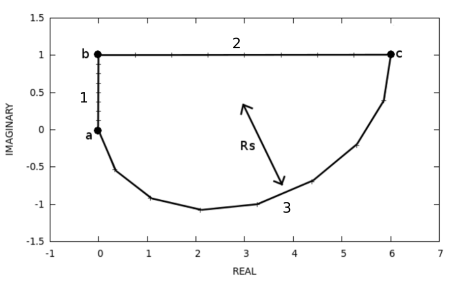
Figure 10: Example contour containing two line segments (pieces 1 and 2) and a half ellipse (piece 3). The secondary radius is half of the primary radius defined by nodes a and c. All the Nc (24) generated Zne points are represented.

7.2.2 Calling the Expert FEAST Routines

There exists an expert version of each FEAST driver and RCI routine. They are signified by an appending “X” and accept the two additional arguments $Zne$ and $Wne$ containing the integration nodes and weights. Below is an example F90 code calling the dense general complex FEAST driver with a custom contour.

⬇

program feast_cc

complex(kind=kind(1.0d0)),dimension(:,:),allocatable :: A, B, X

complex(kind=kind(1.0d0)),dimension(:),allocatable :: E, Zne, Wne, Zedge

complex(kind=kind(1.0d0)) :: Emid

double precision :: r, epsout

integer :: M0, P, info, M, N, LDA, LDB

integer,dimension(64) :: fpm

double precision,dimension(:),allocatable :: res

integer,dimension(:),allocatable :: Nedge, Tedge

allocate(A(1:N,1:N), B(1:N,1:N), E(1:M0), X(1:N,1:2*M0), res(1:2*M0))

… Load A,B

call feastinit(fpm)

… Define Custom Contour - Fill up the P elements of Zedge,Tegde,Nedge

fpm(2) = sum(Nedge(1:P))

allocate(Zne(1:fpm(2)), Wne(1:fpm(2)))

call zfeast_customcontour(fpm(2),P,Nedge,Tedge,Zedge,Zne,Wne) ! generate Zne,Wne

call zfeast_gegvx(N,A,LDA,B,LDA,fpm,epsout,loop,Emid,r,M0,E,X,M,res,info,Zne,Wne)

end program feast_cc

7.3 List of all FEAST tool routines

  - [cz]feast$\_$contour

call zfeast$\_$contour($Emin$, $Emax$, $fpm2$, $fpm16$, $fpm18$, $Zne$, $Wne$)

Inputs:
$Emin$:	Scalar	Type(S,D)	Lower bound of search interval
$Emax$:	Scalar	Type(S,D)	Upper bound of search interval
$fpm2$:	Scalar	Type(I)	Number of contour points for integration (half-contour)
$fpm16$:	Scalar	Type(I)	Integration type
$fpm18$:	Scalar	Type(I)	Ellipse definition
Ouputs:
$Zne$:	Dim($fpm2$)	Type(C,Z)	Integration Nodes (half-contour)
$Wne$:	Dim($fpm2$)	Type(C,Z)	Integration Weights (half-contour)

• Returns FEAST integration nodes and weights for a contour defined by $Emin$ and $Emax$. To be used with complex Hermitian and real symmetric FEAST.

  - [cz]feast$\_$gcontour

call zfeast$\_$gcontour( $Emid$ , $r$ , $fpm8$ , $fpm17$ , $fpm18$ , $fpm19$, $Zne$ , $Wne$ )

Inputs:
$Emid$:	Scalar	Type(C,Z)	Midpoint of search interval
$r$:	Scalar	Type(S,D)	Radius of search interval
$fpm8$:	Scalar	Type(I)	Number of contour points for integration (full contour)
$fpm17$:	Scalar	Type(I)	Integration type
$fpm18$:	Scalar	Type(I)	Ellipse definition
$fpm19$:	Scalar	Type(I)	Ellipse rotation angle
Ouputs:
$Zne$:	Dim($fpm8$)	Type(C,Z)	Integration Nodes (full contour)
$Wne$:	Dim($fpm8$)	Type(C,Z)	Integration Weights (full contour)

• Returns FEAST integration nodes and weights for a contour defined by $Emid$ and $r$. To be used with non-Hermitian FEAST (complex-symmetric, real non-symmetric, general-complex).

  - [cz]feast$\_$customcontour

call zfeast$\_$customcontour( $fpm8$ , $ccN$ , $Nedge$ , $Tedge$ , $Zedge$ , $Zne$ , $Wne$ )

Inputs:
$fpm8$:	Scalar	Type(I)	Number of contour points: sum($Nedge$(1:$ccN$))
$ccN$:	Scalar	Type(I)	Number of segments that comprise contour
$Nedge$:	Dim($ccN$)	Type(I)	Number of contour points for each segment
$Tedge$:	Dim($ccN$)	Type(I)	Type of each segment
$Zedge$:	Dim($ccN$)	Type(C,Z)	Start node of each segment
Outputs:
$Zne$:	Dim($fpm8$)	Type(C,Z)	Integration Nodes
$Wne$:	Dim($fpm8$)	Type(C,Z)	Integration Weights

• Returns FEAST integration nodes and weights for a user defined contour. To be used with FEAST expert routines.

  - [sd]feast$\_$rational

call dfeast$\_$rational( $Emin$ , $Emax$ , $fpm2$ , $fpm16$ , $fpm18$ , $Eig$ , $M0$ , $f$ )

Inputs:
$Emin$:	Scalar	Type(S,D)	Lower bound of search interval
$Emax$:	Scalar	Type(S,D)	Upper bound of search interval
$fpm2$:	Scalar	Type(I)	Number of contour points for integration (half-contour)
$fpm16$:	Scalar	Type(I)	Integration type
$fpm18$:	Scalar	Type(I)	Ellipse definition
$Eig$:	Dim($M0$)	Type(S,D)	Set of points to evaluate rational function
$M0$:	Scalar	Type(I)	Size of $Eig$/$f$
Outputs:
$f$:	Dim($M0$)	Type(S,D)	Value of rational function at each point in Eig

• Evaluates rational/selection function for contour defined by $Emin$ and $Emax$ at a set of real values stored in $Eig$.

  - [sd]feast$\_$rationalx

call dfeast$\_$rationalx( $Zne$ , $Wne$ ,$fpm2$ , $Eig$ , $M0$ , $f$ )

Inputs:
$Zne$:	Dim($fpm2$)	Type(C,Z)	Integration nodes of search interval
$Wne$:	Dim($fpm2$)	Type(C,Z)	Integration Weights of search interval
$fpm2$:	Scalar	Type(I)	Number of contour points for integration (half-contour)
$Eig$:	Dim($M0$)	Type(S,D)	Set of points to evaluate rational function
$M0$:	Scalar	Type(I)	Size of $Eig$/$f$
Outputs:
$f$:	Dim($M0$)	Type(S,D)	Value of rational function at each point in Eig

• Evaluates rational/selection function for contour defined by $Zne$ and $Wne$ at a set of real values stored in $Eig$.

  - [cz]feast$\_$grational

call zfeast$\_$grational( $Emid$ , $r$ , $fpm8$ , $fpm17$ , $fpm18$, $fpm19$ , $Eig$ , $M0$ , $f$ )

Inputs:
$Emid$:	Scalar	Type(C,Z)	Midpoint of search interval
$r$:	Scalar	Type(S,D)	Radius of search interval
$fpm8$:	Scalar	Type(I)	Number of contour points for integration (full-contour)
$fpm17$:	Scalar	Type(I)	Integration type
$fpm18$:	Scalar	Type(I)	Ellipse definition
$fpm19$:	Scalar	Type(I)	Ellipse rotation angle
$Eig$:	Dim($M0$)	Type(C,D)	Set of points to evaluate rational function
$M0$:	Scalar	Type(I)	Size of $Eig$/$f$
Outputs:
$f$:	Dim($M0$)	Type(C,Z)	Value of rational function at each point in Eig

• Evaluates rational/selection function for contour defined by $Emid$ and $r$ at a set of complex values stored in $Eig$.

  - [cz]feast$\_$grationalx

call zfeast$\_$grationalx( $Zne$ , $Wne$ , $fpm8$ , $Eig$ , $M0$ , $f$ )

Inputs:
$Zne$:	Dim($fpm8$)	Type(C,Z)	Integration nodes of search interval
$Wne$:	Dim($fpm8$)	Type(C,Z)	Integration Weights of search interval
$fpm8$:	Scalar	Type(I)	Number of contour points for integration (full contour)
$Eig$:	Dim($M0$)	Type(C,Z)	Set of points to evaluate rational function
$M0$:	Scalar	Type(I)	Size of $Eig$/$f$
Outputs:
$f$:	Dim($M0$)	Type(C,Z)	Value of rational function at each point in Eig

• Evaluates rational/selection function for contour defined by $Zne$ and $Wne$ at a set of complex values stored in $Eig$.