Fast summation by interval clustering for an evolution equation with memory

Abstract

We solve a fractional diffusion equation using a piecewise-constant, discontinuous Galerkin method in time combined with a continuous, piecewise-linear finite element method in space. If there are $N$ time levels and $M$ spatial degrees of freedom, then a direct implementation of this method requires $O(N^{2}M)$ operations and $O(NM)$ storage, owing to the presence of a memory term: at each time step, the discrete evolution equation involves a sum over all previous time levels. We show how the computational cost can be reduced to $O(MN\log N)$ operations and $O(M\log N)$ active memory locations.

1 Introduction

The density $u=u(x,t)$ of particles undergoing anomalous subdiffusion satisfies the integrodifferential equation [7]

$$\frac{\partial u}{\partial t}(x,t)-\nabla\cdot\biggl{(}\frac{\partial}{\partial t}\int_{0}^{t}\frac{(t-s)^{\nu-1}}{\Gamma(\nu)}\,K\nabla u(x,s)\,ds\biggr{)}=f(x,t)$$ (1)

for a parameter $\nu$ in the range $0<\nu<1$, where $K>0$ is a generalized diffusivity and $f$ is a homogeneous term. We consider (1) for $0<t<T$ and for $x$ in a bounded, convex or $C^{2}$ domain $\Omega\subseteq\mathbb{R}^{d}$, subject to homogeneous boundary conditions, either of Dirichlet type,

$$u(x,t)=0\quad\text{for $x\in\partial\Omega$,}$$ (2)

or of Neumann type,

$$\frac{\partial u}{\partial\textnormal{{n}}}(x,t)=0\quad\text{for $x\in\partial\Omega$,}$$ (3)

where n denotes the outward unit normal for $\Omega$. In addition, we specify the initial condition

$$u(x,0)=u_{0}(x)\quad\text{for $x\in\Omega$.}$$

In the limit as $\nu\to 1$, the evolution equation (1) reduces to the classical diffusion equation, $u_{t}-\nabla\cdot(K\nabla u)=f$, in which the flux $-K\nabla u$ depends only on the instantaneous value of the gradient. By contrast, in (1) the flux depends on the entire history of the gradient, and this fact leads to significant computational challenges, particularly if the spatial dimension $d=3$.

In [5], we solved the foregoing initial-boundary value problem using a piecewise-constant, discontinuous Galerkin (DG) method for the time discretization, combined with a standard, continuous piecewise-linear finite element discretization in space. For simplicity, in the present work we assume that both the spatial mesh and the time steps are quasiuniform. Defining the elliptic partial differential operator $Au=-\nabla\cdot(K\nabla u)$, we assume that for some $\sigma\in(0,1]$ the solution $u$ satisfies regularity estimates of the form [4]

$$t^{\nu}\|Au^{\prime}(t)\|+t^{\nu+1}\|Au^{\prime\prime}(t)\|\leq Ct^{\sigma-1}\quad\text{and}\quad\|Au(t)\|+t\|Au^{\prime}(t)\|\leq C$$ (4)

for $0<t\leq T$. The DG solution $U(x,t)$ therefore satisfies an error bound [5, Theorem 3] in the norm of $L_{2}(\Omega)$,

$$\|U^{n}-u(t_{n})\|\leq C(k^{\sigma}+h^{2})\lg(t_{n}/t_{1})\quad\text{for $1\leq m\leq M$ and $1\leq n\leq N$,}$$ (5)

where $t_{n}$ is the $n$th time level, $U^{n}(x)=U(x,t_{n}^{-})$, $k$ is the maximum time step, $h$ is the maximum diameter of the spatial finite elements and $\lg(s)=\max(1,|\log s|)$. When $\sigma<1$, we could achieve full first-order accuracy with respect to $k$ (ignoring logarithmic factors) by relaxing the assumption that the time steps are quasi-uniform, but to do so would complicate our fast solution procedure.

Section 2 provides a precise description of the DG method, which can be interpreted as a type of implicit Euler scheme. Denote the $m$th free node by $x_{m}$, and let $U^{n}_{m}=U(x_{m},t_{n}^{-})$. At the $n$th time step, we compute the vector of nodal values, $\boldsymbol{U}^{n}=[U^{n}_{m}]\in\mathbb{R}^{M}$, by solving a linear system

$$(\boldsymbol{M}+\beta_{nn}\boldsymbol{S})\boldsymbol{U}^{n}=\boldsymbol{M}\boldsymbol{U}^{n-1}+k_{n}\bar{\boldsymbol{f}}^{n}+\boldsymbol{S}\sum_{j=1}^{n-1}\beta_{nj}\boldsymbol{U}^{j}.$$ (6)

Here, $\boldsymbol{M}$ and $\boldsymbol{S}$ are the mass and stiffness matrices arising from the spatial discretization, $k_{n}=t_{n}-t_{n-1}$ is the length of the $n$th time interval, $\bar{f}^{n}$ is the average value of the load vector for $t_{n-1}<t<t_{n}$, and the weights are given by

$$\beta_{nn}=\int_{t_{n-1}}^{t_{n}}\frac{(t_{n}-s)^{\nu-1}}{\Gamma(\nu)}\,ds=\frac{k_{n}^{\nu}}{\Gamma(1+\nu)}$$ (7)

and

$$\beta_{nj}=\int_{t_{j-1}}^{t_{j}}\biggl{(}\frac{(t_{n-1}-s)^{\nu-1}}{\Gamma(\nu)}-\frac{(t_{n}-s)^{\nu-1}}{\Gamma(\nu)}\biggr{)}\,ds>0.$$ (8)

The condition number of the matrix $\boldsymbol{M}+\beta_{nn}\boldsymbol{S}$ is $O(1+k^{\nu}h^{-2})$, and we assume the use of an efficient elliptic solver costing $O(M)$ operations. By comparison, computing the right-hand side in the obvious way requires $O(nM)$ operations. Moreover, we must keep the vector $U^{j}$ in active memory for all the previous time levels $j=1$, $2$, …, $n-1$, requiring $O(nM)$ locations. Thus, the total cost for $N$ time steps is $O(N^{2}M)$ operations and $O(NM)$ active memory locations, whereas applying the same DG method to a classical diffusion equation (which has no memory term) costs only $O(NM)$ operations and $O(M)$ active locations. In other words, solving the fractional diffusion equation in this way costs $N$ times as much as solving a classical diffusion equation.

Cuesta, Lubich and Palencia [1] studied the time discretization of (1) by convolution quadrature, and Schädle, López-Fernández and Lubich [8, 2] developed a fast solution algorithm costing $O(MN\log N)$ operations and using $O(M\log N)$ active memory locations. The purpose of this paper is to present a fast summation algorithm for the DG method (6) that likewise costs $O(MN\log N)$ operations and $O(M\log N)$ active memory locations.

The algorithm is closely related to the panel clustering technique for boundary element methods, introduced by Hackbusch and Nowak [3]. To explain the basic strategy, suppose that instead of $(t-s)^{\nu-1}/\Gamma(\nu)$ the integral term had a degenerate kernel $\sum_{p=1}^{r}a_{p}(t)b_{p}(s)$. In this case,

$$\beta_{nj}=\sum_{p=1}^{r}\phi_{pn}\psi_{pj}\quad\text{for $1\leq j\leq n\leq N$,}$$ (9)

where $\phi_{np}=a_{p}(t_{n})-a_{p}(t_{n-1})$ and $\psi_{nj}=\int_{t_{j-1}}^{t_{j}}b_{p}(s)\,ds$. Since

$$\sum_{j=1}^{n-1}\beta_{nj}\boldsymbol{U}^{j}=\sum_{p=1}^{r}\phi_{pn}\Psi^{n-1}_{p}(\boldsymbol{U})\quad\text{where}\quad\Psi^{n-1}_{p}(\boldsymbol{U})=\sum_{j=1}^{n-1}\psi_{pj}\boldsymbol{U}^{j},$$

and since $\Psi^{n}_{p}(\boldsymbol{U})=\Psi^{n-1}_{p}(\boldsymbol{U})+\psi_{pn}\boldsymbol{U}^{n}$, evaluating the right-hand side of the linear system (6) would cost only $O(rM)$ operations and there would be no need to retain in active memory the solution at all previous time levels. Our kernel $(t-s)^{\nu-1}/\Gamma(\nu)$ is not degenerate, but it can be approximated to high accuracy by a degenerate kernel if we restrict $t$ and $s$ to suitable, well-separated intervals. Consequently, if $t_{n}$ and $t_{j}$ are restricted in the same way, then $\beta_{nj}$ can be approximated to high accuracy by a sum $\tilde{\beta}_{nj}$ of the form (9), leading to a fast method to evaluate the sum that occurs on the right-hand side of (6).

In Section 2 we investigate the effect of perturbing the DG method in this way, and Section 3 presents a simple scheme for generating the $\tilde{\beta}_{nj}$ via Taylor expansion. Section 4 describes the cluster tree, whose nodes are contiguous families of time intervals, used to appropriately restrict $t_{n}$ and $t_{j}$. The fast summation algorithm is then defined via the concept of an admissible covering, and we present an error estimate in Theorem 4.3. Further investigation of the cluster tree in Section 5 allows us to prove, in Theorem 5.3, that the algorithm requires $O(NM\log N)$ operations. In Section 6, we present a memory management strategy and show, in Theorem 6.1, that with this strategy the fast summation algorithm uses at most $O(M\log N)$ active memory locations during each time step. Section 7 presents a numerical example, and the paper concludes with three technical appendices.

Although presented here only for equation (1) discretized in time using a piecewise-constant DG method, the fast summation algorithm does not depend in any essential way on this specific choice and could be used for many other time stepping procedures for evolution problems with memory. The key requirements are that the quadrature weights are computed via local averages of the kernel and that, away from the diagonal, the derivatives of the kernel exist and decay appropriately. Also, the approximation scheme of Section 3, based on Taylor expansions, is only one possibility, chosen because it is simple to analyse for the kernel in (1). We could instead use an interpolation scheme that requires a user to supply only pointwise values of the kernel.

2 Numerical method

We define $\omega_{\nu}(t)=t^{\nu-1}/\Gamma(\nu)$ and denote the Riemann–Liouville fractional differentiation operator of order $1-\nu$ by

$$\mathcal{B}v(t)=(\omega_{\nu}*v)_{t}=\frac{\partial}{\partial t}\int_{0}^{t}\omega_{\nu}(t-s)v(s)\,ds,$$

and let $u_{t}=\partial u/\partial t$ so that, suppressing the dependence on $x$,

$$u_{t}+\mathcal{B}Au=f(t)\quad\text{for $0<t<T$, with $u(0)=u_{0}$.}$$ (10)

We also denote the inner product in $L_{2}(\Omega)$ and the bilinear form associated with $A$ by

$$\langle u,v\rangle=\int_{\Omega}uv\,dx\quad\text{and}\quad\textsf{A}(u,v)=\int_{\Omega}K\nabla u\cdot\nabla v\,dx.$$

The weak form of (10) is then

$$\langle u_{t},v\rangle+\textsf{A}(\mathcal{B}u,v)=\langle f(t),v\rangle\quad\text{for all test functions~{}$v\in L_{2}\bigl{(}(0,T),\dot{H}^{1}\bigr{)}$,}$$

where $\dot{H}^{1}$ is the Sobolev space $H^{1}_{0}(\Omega)$ in the case of Dirichlet boundary conditions (2), and $H^{1}(\Omega)$ in the case of Neumann boundary conditions (3).

The numerical solution $U(t)\approx u(t)$ is a piecewise-constant function of $t$, with coefficients belonging to a continuous, piecewise-linear finite element space $S_{h}\subseteq\dot{H}^{1}$. Thus, $U$ generally has a jump discontinuity at each time level $t_{n}$, and we adopt the usual convention of treating $U(t)$ as continuous for $t$ in the half-open interval $I_{n}=(t_{n-1},t_{n}]$, writing

$$U^{n}=U(t_{n})=U(t_{n}^{-}),\qquad U^{n}_{+}=U(t_{n}^{+}),\qquad[U]^{n}=U^{n}_{+}-U^{n}.$$

The DG time-stepping procedure is determined by the variational equation

$$\langle U^{n-1}_{+},V^{n-1}_{+}\rangle+\int_{I_{n}}\bigl{[}\langle U^{\prime}(t),V(t)\rangle+A\bigl{(}\mathcal{B}U(t),V(t)\bigr{)}\bigr{]}\,dt\\ =\langle U^{n-1},V^{n-1}_{+}\rangle+\int_{I_{n}}\langle f(t),V(t)\rangle\,dt,$$

which must hold for every piecewise-constant test function $V$ with coefficients in $S_{h}$. In our piecewise-constant case, $U^{n-1}_{+}=U^{n}$ so this variational equation reduces to finding $U^{n}\in S_{h}$ such that

$$\biggl{\langle}\frac{U^{n}-U^{n-1}}{k_{n}},\chi\biggr{\rangle}+\textsf{A}\bigl{(}\bar{\mathcal{B}}^{n}U,\chi\bigr{)}=\langle\bar{f}^{n},\chi\rangle\quad\text{for all $\chi\in S_{h}$,}$$

where $\bar{f}^{n}=k_{n}^{-1}\int_{I_{n}}f(t)\,dt$ and

$$\bar{\mathcal{B}}^{n}U=\frac{1}{k_{n}}\int_{I_{n}}\mathcal{B}U(t)\,dt=\frac{1}{k_{n}}\biggl{(}\beta_{nn}U^{n}-\sum_{j=1}^{n-1}\beta_{nj}U^{j}\biggr{)}.$$ (11)

Thus, the vector of nodal values of $U^{n}$ satisfies (6), with weights given by (7) and (8).

Our fast algorithm approximates $\bar{\mathcal{B}}^{n}U$ with

$$\widetilde{\mathcal{B}}^{n}U=\frac{1}{k_{n}}\biggl{(}\beta_{nn}U^{n}-\sum_{j=1}^{n-1}\tilde{\beta}_{nj}U^{j}\biggr{)},$$ (12)

where $\tilde{\beta}_{nj}\approx\beta_{nj}$ for $1\leq j\leq n-1$, and yields $\tilde{U}^{n}$ satisfying the perturbed equation

$$\biggl{\langle}\frac{\tilde{U}^{n}-\tilde{U}^{n-1}}{k_{n}},\chi\biggr{\rangle}+\textsf{A}\bigl{(}\widetilde{\mathcal{B}}^{n}\tilde{U},\chi\bigr{)}=\langle\bar{f}^{n},\chi\rangle\quad\text{for all $\chi\in S_{h}$,}$$ (13)

with $\tilde{U}^{0}=U^{0}$.

Theorem 2.1.

If, for every real-valued, piecewise-constant function $V$,

$$\sum_{n=1}^{N}k_{n}(\widetilde{\mathcal{B}}^{n}V)V^{n}\geq 0,$$ (14)

then the perturbed problem (13) is stable:

$$\|\tilde{U}^{n}\|\leq\|\tilde{U}^{0}\|+2\sum_{j=1}^{n}k_{j}\|\bar{f}^{j}\|\quad\text{for $1\leq n\leq N$.}$$

Proof.

This estimate follows by a simple energy argument [5, Theorem 1]. ∎

In Appendix A, we prove a lower bound

$$\sum_{n=1}^{N}k_{n}(\bar{\mathcal{B}}^{n}V)V^{n}\geq\rho_{\nu}T^{\nu-1}\sum_{n=1}^{N}k_{n}(V^{n})^{2},$$ (15)

where the constant $\rho_{\nu}>0$ depends only on $\nu$, allowing us to show the following.

Corollary 2.2.

The perturbed DG method (13) is stable if

$$\sum_{j=1}^{n-1}|\tilde{\beta}_{nj}-\beta_{nj}|\leq\rho_{\nu}T^{\nu-1}k_{n}\quad\text{for $2\leq n\leq N$,}$$

and

$$\sum_{n=j+1}^{N}|\tilde{\beta}_{nj}-\beta_{nj}|\leq\rho_{\nu}T^{\nu-1}k_{j}\quad\text{for $1\leq j\leq N-1$.}$$

Proof.

Write

$$\Delta=\sum_{n=1}^{N}k_{n}(\widetilde{\mathcal{B}}^{n}V)V^{n}-\sum_{n=1}^{N}k_{n}(\bar{\mathcal{B}}^{n}V)V_{n}=\sum_{n=2}^{N}\sum_{j=1}^{n-1}(\beta_{nj}-\tilde{\beta}_{nj})V_{j}V_{n},$$

and observe that since $|V^{j}V^{n}|\leq\tfrac{1}{2}(V^{j})^{2}+\tfrac{1}{2}(V^{n})^{2}$,

$$|\Delta|\leq\frac{1}{2}\sum_{j=1}^{N-1}(V^{j})^{2}\sum_{n=j+1}^{N}|\tilde{\beta}_{nj}-\beta_{nj}|+\frac{1}{2}\sum_{n=2}^{N}(V^{n})^{2}\sum_{j=1}^{n-1}|\tilde{\beta}_{nj}-\beta_{nj}|\\ \leq\rho_{\nu}T^{\nu-1}\sum_{n=1}^{N}k_{n}(V^{n})^{2}.$$

∎

To estimate the effect on the solution $U^{n}$ of perturbing the weights $\beta_{nj}$, we introduce the piecewise-constant interpolation operator

$$\Pi u(t)=u(t_{n})\quad\text{for $t_{n-1}<t\leq t_{n}$.}$$

In the next result, for simplicity we treat the semi-discrete DG method in which there is no spatial discretization; the fully-discrete method could be analysed using the methods of McLean and Mustapha [5, Section 5].

Theorem 2.3.

Assume that $S_{h}=\dot{H}^{1}$ and $\tilde{U}^{0}=u_{0}$. If the perturbed equation (13) is stable, and if

$$\sum_{j=1}^{n}\sum_{l=1}^{j-1}|\tilde{\beta}_{jl}-\beta_{jl}|\leq\epsilon_{n},$$

then

$$\|\tilde{U}^{n}-u(t_{n})\|\leq 2\epsilon_{n}\max_{1\leq j\leq n-1}\|Au(t_{j})\|+2\sum_{j=1}^{n}k_{j}\|\bar{\mathcal{B}}^{n}A(u-\Pi u)\|.$$ (16)

Proof.

Since $\tilde{U}$ satisfies (13) and $u$ satisfies

$$\biggl{\langle}\frac{u(t_{n})-u(t_{n-1})}{k_{n}},\chi\biggr{\rangle}+\textsf{A}\bigl{(}\bar{\mathcal{B}}^{n}u,\chi\bigr{)}=\langle\bar{f}^{n},\chi\rangle\quad\text{for all $\chi\in S_{h}$,}$$

the difference $W^{n}=\tilde{U}^{n}-U^{n}$ satisfies

$$\biggl{\langle}\frac{W^{n}-W^{n-1}}{k_{n}},\chi\biggr{\rangle}+\textsf{A}\bigl{(}\widetilde{\mathcal{B}}^{n}W,\chi\bigr{)}=\langle\bar{g}^{n},\chi\rangle\quad\text{for all $\chi\in S_{h}$,}$$

where $\bar{g}^{n}=\bigl{(}\bar{\mathcal{B}}^{n}-\widetilde{\mathcal{B}}^{n}\bigr{)}\Pi Au+\bar{\mathcal{B}}^{n}A(u-\Pi u)$. Noting that $W^{0}=0$, stability of the perturbed equation implies that

$$\|W^{n}\|\leq 2\sum_{j=1}^{n}k_{j}\|\bar{g}^{n}\|,$$

and from (11) and (12) we see that

$$\bigl{(}\bar{\mathcal{B}}^{j}-\widetilde{\mathcal{B}}^{j}\bigr{)}\Pi Au=k_{j}^{-1}\sum_{l=1}^{j-1}\bigl{(}\tilde{\beta}_{jl}-\beta_{jl}\bigr{)}Au(t_{j}).$$

∎

The second term on the right-hand side of (16) does not involve $\tilde{\beta}_{nj}$ and is $O(k^{\sigma})$ [5].

3 Taylor approximation of the weights

Recall from (7) that $\beta_{nn}=\omega_{1+\nu}(k_{n})$, and from (8) that for $1\leq j\leq n-1$,

$$\beta_{nj}=\int_{I_{j}}\bigl{[}\omega_{\nu}(t_{n-1}-s)-\omega_{\nu}(t_{n}-s)\bigr{]}\,ds=-\int_{I_{j}}\int_{I_{n}}\omega_{\nu-1}(t-s)\,dt\,ds.$$ (17)

Denote the midpoint of the interval $I_{n}$ by $t_{n-1/2}=\tfrac{1}{2}(t_{n-1}+t_{n})$, and define

$$B_{\mu}(t,k)=\int_{-k/2}^{k/2}\omega_{\mu}(t+s)\,ds=\omega_{1+\mu}(t+\tfrac{1}{2}k)-\omega_{1+\mu}(t-\tfrac{1}{2}k)$$

for $t>k/2$ and $-\infty<\mu<\infty$. The approximate weights $\tilde{\beta}_{nj}$ are determined as follows. See Appendices B and C for notes on the stable evaluation of these quantities.

Theorem 3.1.

Let $0<\eta\leq 1$ and suppose that $0\leq a<b<c<d\leq T$ with

$$I_{j}\subseteq(a,b],\qquad I_{n}\subseteq(c,d],\qquad\frac{b-a}{c-b}\leq\eta.$$ (18)

Denote the midpoint of $[a,b]$ by $\bar{s}=\tfrac{1}{2}(a+b)$, and define

$$\phi_{pn}=(-1)^{p}B_{\nu-p}(t_{n-1/2}-\bar{s},k_{n}),\qquad\psi_{pj}=B_{p}(t_{j-1/2}-\bar{s},k_{j}),$$

and

$$\tilde{\beta}_{nj}=\sum_{p=1}^{r}\phi_{pn}\psi_{pj}.$$

Then

$$|\tilde{\beta}_{nj}-\beta_{nj}|\leq 2^{2-\nu}(r+1)(\eta/2)^{r}\beta_{nj}.$$

Proof.

Taylor expansion about $\bar{s}$ gives

$$\omega_{\nu-1}(t-s)=\sum_{p=0}^{r-1}(-1)^{p}\omega_{\nu-1-p}(t-\bar{s})\omega_{1+p}(s-\bar{s})\\ +(-1)^{r}\int_{\bar{s}}^{s}\omega_{r}(s-y)\omega_{\nu-1-r}(t-y)\,dy,$$

so, by (17), integrating over $t\in I_{n}$ and $s\in I_{j}$ gives $\beta_{nj}=\tilde{\beta}_{nj}+E_{rnj}$ with

$$E_{rnj}=(-1)^{r+1}\int_{I_{n}}\int_{I_{j}}\int_{\bar{s}}^{s}\omega_{r}(s-y)\omega_{\nu-1-r}(t-y)\,dy\,ds\,dt.$$

Since $y\in I_{j}\subseteq(a,b]$ and $t\in I_{n}\subseteq(c,d]$, we have $t-y\geq c-b$, so

$$|E_{rnj}|\leq\frac{(c-b)^{-r}}{|\Gamma(\nu-r-1)|}\int_{I_{n}}\int_{I_{j}}\frac{|s-\bar{s}|^{r-1}}{r!}\biggl{|}\int_{\bar{s}}^{s}\frac{dy}{(t-y)^{2-\nu}}\biggr{|}\,ds\,dt.$$

If $\bar{s}\leq s$, then $y\leq s$ so $t-y\geq t-s$. However, if $s\leq\bar{s}$ then $0\leq y-s\leq\bar{s}-s\leq\tfrac{1}{2}(b-a)$ so

$$t-y=(t-s)-(y-s)\geq(t-s)-\tfrac{1}{2}(b-a)=(t-s)\biggl{(}1-\frac{\tfrac{1}{2}(b-a)}{t-s}\biggr{)}.$$

Also, $t-s\geq c-b$ because $s\in[a,b]$, and assumption (18) implies that $t-y\geq(t-s)(1-\tfrac{1}{2}\eta)$. Thus,

$$\biggl{|}\int_{\bar{s}}^{s}\frac{dy}{(t-y)^{2-\nu}}\,dy\biggr{|}\leq\frac{1}{(1-\tfrac{1}{2}\eta)^{2-\nu}}\,\frac{|s-\bar{s}|}{(t-s)^{2-\nu}},$$

and since $|s-\bar{s}|\leq\tfrac{1}{2}(b-a)\leq\tfrac{1}{2}\eta(c-b)$, it follows that

$$|E_{rnj}|\leq\biggl{(}\frac{2}{2-\eta}\biggr{)}^{2-\nu}\frac{(\eta/2)^{r}}{r!|\Gamma(\nu-r-1)|}\int_{I_{n}}\int_{I_{j}}\frac{ds\,dt}{(t-s)^{2-\nu}}.$$

The identity $\Gamma(\nu-1)=(\nu-2)(\nu-3)\cdots(\nu-r)(\nu-r-1)\Gamma(\nu-r-1)$ shows that

$$\biggl{|}\frac{\Gamma(\nu-1)}{r!\Gamma(\nu-r-1)}\biggr{|}\leq\frac{2-\nu}{2}\,\frac{3-\nu}{3}\cdots\frac{r-\nu}{r}\,(r+1-\nu)\leq r+1,$$

and because $\Gamma(\nu-1)=\Gamma(\nu)/(\nu-1)<0$,

$$|E_{rnj}|\leq 2^{2-\nu}(r+1)(\eta/2)^{r}\biggl{(}-\int_{I_{n}}\int_{I_{j}}\frac{(t-s)^{\nu-2}}{\Gamma(\nu-1)}\,ds\,dt\biggr{)}.$$

∎

Whereas $\psi_{pj}$ depends on $[a,b]$ (via $\bar{s}$), in the following alternative expansion $\psi^{\star}_{pj}$ depends only on $p$ and $j$. However, the sum that defines $\phi_{pn}^{\star}$ is susceptible to loss of precision.

Corollary 3.2.

If we define

$$\phi_{pn}^{\star}=\sum_{q=p}^{r}\frac{(-\bar{s})^{q-p}}{(q-p)!}\,\phi_{qn}\quad\text{and}\quad\psi_{pj}^{\star}=B_{p}(t_{j-1/2},k_{j}),$$

then

$$\tilde{\beta}_{nj}=\sum_{p=0}^{r}\phi^{\star}_{pn}\psi^{\star}_{pj}.$$

Proof.

The binomial expansion gives

$$\psi_{pj}=\int_{I_{j}}\frac{(s-\bar{s})^{p-1}}{(p-1)!}\,ds=\sum_{q=1}^{p}\frac{(-\bar{s})^{p-q}}{(p-q)!}\int_{I_{j}}\frac{s^{q-1}}{(q-1)!}\,ds$$

so

$$\tilde{\beta}_{nj}=\sum_{q=1}^{r}\biggl{(}\sum_{p=q}^{r}\phi_{pn}\,\frac{(-\bar{s})^{p-q}}{(p-q)!}\biggr{)}\int_{I_{j}}\frac{s^{q-1}}{(q-1)!}\,ds.$$

∎

4 Cluster tree

We introduce the notation

$$\textnormal{{C}}(j,n)=\{I_{j},I_{j+1},\ldots,I_{n}\}\quad\text{for $1\leq j\leq n\leq N$,}$$

and refer to any such set of consecutive subintervals as a cluster. A cluster tree for the mesh $0=t_{0}<t_{1}<\cdots<t_{N}=T$ is a tree $\mathcal{T}$ having the following properties:

1. each node of $\mathcal{T}$ is a cluster;

2. the root node of $\mathcal{T}$ is $\textnormal{{C}}(1,N)$;

3. each node is either a leaf or else equals the disjoint union of its children.

Let $\mathcal{L}$ denote the set of leaves in the cluster tree $\mathcal{T}$, and observe that for any two distinct nodes $\textnormal{{C}}_{1}\neq\textnormal{{C}}_{2}$ of $\mathcal{T}$ exactly one of the following holds [3, Remark 3.4]: $\textnormal{{C}}_{1}\subsetneq\textnormal{{C}}_{2}$; $\textnormal{{C}}_{2}\subsetneq\textnormal{{C}}_{1}$; or $\textnormal{{C}}_{1}\cap\textnormal{{C}}_{2}=\emptyset$.

In the obvious way, we define the length of a cluster C to be the length of the underlying interval $\bigcup\textnormal{{C}}$; thus,

$$\operatorname{Len}(\textnormal{{C}})=t_{n}-t_{j-1}\quad\text{if $\textnormal{{C}}=\textnormal{{C}}(j,n)$.}$$

The distance between two clusters is the Euclidean distance between the underlying point sets in $\mathbb{R}$,

$$\operatorname{Dist}(\textnormal{{C}}_{1},\textnormal{{C}}_{2})=\inf\{\,|t-s|:\text{$t\in\textstyle{\bigcup\textnormal{{C}}_{1}}$ and $s\in\textstyle{\bigcup\textnormal{{C}}_{2}}$}\,\},$$

so in particular, $\operatorname{Dist}\bigl{(}\textnormal{{C}}(j_{1},n_{1}),\textnormal{{C}}(j_{2},n_{2})\bigr{)}=t_{j_{2}-1}-t_{n_{1}}$ if $j_{2}>n_{1}$. We define the history of a cluster to be the entire preceding half-open interval:

$$\operatorname{History}(\textnormal{{C}})=(0,t_{j-1}]\quad\text{if $\textnormal{{C}}=\textnormal{{C}}(j,n)$.}$$

Given a leaf $\textnormal{{L}}\in\mathcal{L}$, and a parameter $\eta$ in the range $0<\eta\leq 1$, we say that a cluster C is $(\textnormal{{L}},\eta)$-admissable if

$$\bigcup\textnormal{{C}}\subseteq\operatorname{History}(\textnormal{{L}})\quad\text{and}\quad\operatorname{Len}(\textnormal{{C}})\leq\eta\operatorname{Dist}(\textnormal{{C}},\textnormal{{L}}).$$

Thus, the conclusions of Theorem 3.1 hold for $I_{j}\in\textnormal{{C}}$ and $I_{n}\in\textnormal{{L}}$ with $\bigcup\textnormal{{C}}=(a,b]$ and $\bigcup\textnormal{{L}}=(c,d]$. Notice that if C is $(\textnormal{{L}},\eta)$-admissible, then so are all the descendents of C.

An $(\textnormal{{L}},\eta)$-admissible cover is a set $\mathcal{C}$ of clusters such that

1. each cluster $\textnormal{{C}}\in\mathcal{C}$ is a node of $\mathcal{T}$;

2. $\bigcup\{\,I:I\in\textnormal{{C}}\in\mathcal{C}\,\}=\operatorname{History}(\textnormal{{L}})$;

3. if $\textnormal{{C}}_{1}$, $\textnormal{{C}}_{2}\in\mathcal{C}$ with $\textnormal{{C}}_{1}\neq\textnormal{{C}}_{2}$, then $\textnormal{{C}}_{1}\cap\textnormal{{C}}_{2}=\emptyset$;

4. if $\textnormal{{C}}\in\mathcal{C}$ then either C is $(\textnormal{{L}},\eta)$-admissible, or else $\textnormal{{C}}\in\mathcal{L}$.

A trivial example of an $(\textnormal{{L}},\eta)$-admissible cover is the set of leaves in the history of L, that is,

$$\mathcal{C}=\{\,\textnormal{{L}}^{\prime}\in\mathcal{L}:\textnormal{{L}}^{\prime}\subseteq\operatorname{History}(\textnormal{{L}})\}.$$

Lemma 4.1.

All $(\textnormal{{L}},\eta)$-admissible covers contain the same non-admissible leaves.

Proof.

Let $\mathcal{C}_{1}$ and $\mathcal{C}_{2}$ be $(\textnormal{{L}},\eta)$-admissible covers, and suppose that $\textnormal{{L}}^{\prime}\in\mathcal{C}_{1}\cap\mathcal{L}$ is not $(\textnormal{{L}},\eta)$-admissible. Since $\textnormal{{L}}^{\prime}\subseteq\operatorname{History}(\textnormal{{L}})=\bigcup\{\,I:I\in\textnormal{{C}}\in\mathcal{C}_{2}\,\}$, there exist $I\in\textnormal{{C}}\in\mathcal{C}_{2}$ such that $I$ intersects at least one interval $I^{\prime}\in\textnormal{{L}}^{\prime}$. Since $\textnormal{{L}}^{\prime}$ is a leaf of $\mathcal{T}$, it follows that $\textnormal{{L}}^{\prime}\subseteq\textnormal{{C}}$ and hence C is not $(\textnormal{{L}},\eta)$-admissible. Thus, C must be a leaf, because $\mathcal{C}_{2}$ is an $(\textnormal{{L}},\eta)$-admissible cover, and we conclude that $\textnormal{{C}}=\textnormal{{L}}^{\prime}$. ∎

Algorithm 4.1 defines a recursive procedure, $\textsl{divide}(\textnormal{{C}},\mathcal{C},\textnormal{{L}},\eta)$, that we use to define a family of clusters $\mathcal{M}(\textnormal{{L}})$, as follows:

  $\textnormal{{C}}=\textnormal{{C}}(1,N)$, $\mathcal{C}=\emptyset$

  $\textsl{divide}(\textnormal{{C}},\mathcal{C},\textnormal{{L}},\eta)$

  $\mathcal{M}(\textnormal{{L}})=\mathcal{C}$

This construction is a modified version of [3, (3.8b)].

Theorem 4.2.

$\mathcal{M}(\textnormal{{L}})$ is the unique minimal $(\textnormal{{L}},\eta)$-admissible cover.

Proof.

Suppose that $\mathcal{C}$ is an $(\textnormal{{L}},\eta)$-admissible cover. Let $\textnormal{{M}}\in\mathcal{M}(\textnormal{{L}})$ and let C be any node of $\mathcal{C}$ that intersects M. If M is a leaf, then M is not $(L,\eta)$-admissible so $\textnormal{{M}}=\textnormal{{C}}$ by Lemma 4.1. If M is not a leaf, then either C is a leaf, in which case $\textnormal{{C}}\subsetneq\textnormal{{M}}$, or else C is $(\textnormal{{L}},\eta)$-admissible and $\textnormal{{C}}\subseteq\textnormal{{M}}$ by the construction of $\mathcal{M}(\textnormal{{L}})$ using Algorithm 4.1. Hence, in all cases $\textnormal{{C}}\subseteq\textnormal{{M}}$, so either $\mathcal{C}=\mathcal{M}(\textnormal{{L}})$ or else $\#\mathcal{M}(\textnormal{{L}})<\#\mathcal{C}$. ∎

Algorithm 4.1 $\textsl{divide}(\textnormal{{C}},\mathcal{C},\textnormal{{L}},\eta)$

  Determine $a$, $b$, $c$, $d$ such that $\bigcup\textnormal{{C}}=(a,b]$ and $\bigcup\textnormal{{L}}=(c,d]$

  $\mathcal{C}=\emptyset$

  if $a\leq c$ then

     if $b\leq c$ and $b-a\leq\eta(c-b)$ then {C is $(\textnormal{{L}},\eta)$-admissible}

        $\mathcal{C}=\mathcal{C}\cup\{\textnormal{{C}}\}$

     else if $b\leq c$ and $\textnormal{{C}}\in\mathcal{L}$ then

        $\mathcal{C}=\mathcal{C}\cup\{\textnormal{{C}}\}$

     else

        for all $\textnormal{{C}}^{\prime}\in\operatorname{Children}(\textnormal{{C}})$ do

           $\textsl{divide}(\textnormal{{C}}^{\prime},\mathcal{C},\textnormal{{L}},\eta)$

        end for

     end if

  end if

The minimal admissible cover $\mathcal{M}(\textnormal{{L}})$ is the disjoint union of the sets

$$\operatorname{Near}(\textnormal{{L}}) =\{\,\textnormal{{C}}\in\mathcal{M}(\textnormal{{L}}):\text{$\textnormal{{C}}$ is not $(\textnormal{{L}},\eta)$-admissible}\,\},$$ (19)

$$\operatorname{Far}(\textnormal{{L}}) =\{\,\textnormal{{C}}\in\mathcal{M}(\textnormal{{L}}):\text{$\textnormal{{C}}$ is $(\textnormal{{L}},\eta)$-admissible}\,\}.$$

Given $n$, there is a unique leaf $\textnormal{{L}}=\textnormal{{L}}_{n}$ containing $I_{n}$, and we define $\phi_{pn}(\textnormal{{C}})$ and $\psi_{pn}(\textnormal{{C}})$ using the formulae of Theorem 3.1 with $(a,b]=\bigcup\textnormal{{C}}$ and $(c,d]=\bigcup\textnormal{{L}}_{n}$. We then define

$$\tilde{\beta}_{nj}=\beta_{nj}\quad\text{if $I_{j}\in\textnormal{{L}}_{n}$ or $I_{j}\in\textnormal{{C}}\in\operatorname{Near}(\textnormal{{L}}_{n})$,}$$ (20)

and

$$\tilde{\beta}_{nj}=\sum_{p=1}^{r}\phi_{pn}(\textnormal{{C}})\psi_{pj}(\textnormal{{C}})\quad\text{if $I_{j}\in\textnormal{{C}}\in\operatorname{Far}(\textnormal{{L}}_{n})$,}$$ (21)

so that

$$\sum_{j=1}^{n-1}\tilde{\beta}_{nj}V^{j}=\Sigma_{n}(\textnormal{{L}}_{n},V)+\sum_{\textnormal{{C}}\in\operatorname{Near}(\textnormal{{L}}_{n})}\Sigma_{n}(\textnormal{{C}},V)+\sum_{\textnormal{{C}}\in\operatorname{Far}(\textnormal{{L}}_{n})}\widetilde{\Sigma}_{n}(\textnormal{{C}},V),$$ (22)

where

$$\Sigma_{n}(\textnormal{{C}},V)=\sum_{\begin{subarray}{c}I_{j}\in\textnormal{{C}}\\ j\leq n-1\end{subarray}}\beta_{nj}V^{j}\quad\text{and}\quad\widetilde{\Sigma}_{n}(\textnormal{{C}},V)=\sum_{I_{j}\in\textnormal{{C}}}\tilde{\beta}_{nj}V^{j}.$$

To evaluate $\widetilde{\Sigma}_{n}(\textnormal{{C}},V)$, we compute

$$\widetilde{\Sigma}_{n}(\textnormal{{C}},V)=\sum_{p=1}^{r}\phi_{pn}(\textnormal{{C}})\Psi_{p}(\textnormal{{C}},V)\quad\text{where}\quad\Psi_{p}(\textnormal{{C}},V)=\sum_{I_{j}\in\textnormal{{C}}}\psi_{pj}(\textnormal{{C}})V^{j}.$$

The results of Sections 2 and 3 now yield the following estimate for the additional error incurred by using the approximating sum (22). Recall that $\rho_{\nu}$ is the constant appearing in the lower bound (15).

Theorem 4.3.

Define $\tilde{\beta}_{nj}$ according to Theorem 3.1, (20) and (21), and put $k_{\min}=\min_{1\leq n\leq N}k_{n}$. The perturbed problem (13) is stable if

$$(r+1)(\eta/2)^{r}\leq 2^{\nu-2}\Gamma(\nu+1)\rho_{\nu}(k_{\min}/T)^{1-\nu},$$

in which case the error estimate (16) for the semidiscrete DG method holds with

$$\epsilon_{n}=\frac{2^{2-\nu}}{\Gamma(\nu+1)}\,(r+1)(\eta/2)^{r}nk^{\nu}\quad\text{for $1\leq n\leq N$.}$$

Proof.

Recalling (8), we have

$$\sum_{j=1}^{n-1}\beta_{nj} =\int_{0}^{t_{n-1}}\biggl{(}\frac{(t_{n-1}-s)^{\nu-1}}{\Gamma(\nu)}-\frac{(t_{n}-s)^{\nu-1}}{\Gamma(\nu)}\biggr{)}\,ds$$

$$=\frac{k_{n}^{\nu}-\bigl{(}t_{n}^{\nu}-t_{n-1}^{\nu}\bigr{)}}{\Gamma(\nu+1)}\leq\frac{k_{n}^{\nu}}{\Gamma(\nu+1)}$$

and

$$\sum_{n=j+1}^{N}\beta_{nj} =\int_{t_{j-1}}^{t_{j}}\frac{(t_{j}-s)^{\nu-1}-(T-s)^{\nu-1}}{\Gamma(\nu)}\,ds$$

$$=\frac{k_{j}^{\nu}-[(T-t_{j-1})^{\nu}-(T-t_{j})^{\nu}]}{\Gamma(\nu+1)}\leq\frac{k_{j}^{\nu}}{\Gamma(\nu+1)}.$$

Thus, by Theorem 3.1,

$$\sum_{j=1}^{n-1}\bigl{|}\tilde{\beta}_{nj}-\beta_{nj}\bigr{|}\leq 2^{2-\nu}(r+1)(\eta/2)^{r}\,\frac{k_{n}^{\nu}}{\Gamma(\nu+1)}$$

and

$$\sum_{n=j+1}^{N}\bigl{|}\tilde{\beta}_{nj}-\beta_{nj}\bigr{|}\leq 2^{2-\nu}(r+1)(\eta/2)^{r}\,\frac{k_{j}^{\nu}}{\Gamma(\nu+1)}.$$

Therefore, Corollary 2.2 shows that the perturbed scheme is stable if

$$2^{2-\nu}(r+1)(\eta/2)^{r}\,\frac{k_{n}^{\nu}}{\Gamma(\nu+1)}\leq\rho_{\nu}T^{\nu-1}k_{n}\quad\text{for $1\leq n\leq N$,}$$

and since

$$\sum_{j=1}^{n}\sum_{l=1}^{j-1}|\tilde{\beta}_{nj}-\beta_{n}j|\leq 2^{2-\nu}(r+1)(\eta/2)^{r}\sum_{j=1}^{n}\frac{k_{j}^{\nu}}{\Gamma(\nu+1)},$$

the error bound follows at once from Theorem 2.3. ∎

Since $N^{-1}\leq Ck_{\min}/T$ because the mesh is quasiuniform, we have stability if $(r+1)(\eta/2)^{r}\leq CN^{\nu-1}$, and the error factor satisfies

$$\epsilon_{n}=O(k)\quad\text{if}\quad(r+1)(\eta/2)^{r}\leq CN^{\nu-2}.$$ (23)

The alternative expansion from Corollary 3.2 gives $\phi_{pn}^{\star}(\textnormal{{C}})$ and $\psi_{pj}^{\star}$ such that

$$\tilde{\beta}_{nj}=\sum_{p=1}^{r}\phi_{pn}^{\star}(\textnormal{{C}})\psi_{pj}^{\star}\quad\text{if $I_{j}\in\textnormal{{C}}\in\operatorname{Far}(\textnormal{{L}}_{n})$,}$$

so

$$\widetilde{\Sigma}_{n}(\textnormal{{C}},V)=\sum_{p=1}^{r}\phi_{pn}^{\star}(\textnormal{{C}})\Psi_{p}^{\star}(\textnormal{{C}},V)\quad\text{where}\quad\Psi_{p}^{\star}(\textnormal{{C}},V)=\sum_{I_{j}\in\textnormal{{C}}}\psi_{pj}^{\star}V^{j}.$$

If C is not a leaf, then C is the union of its children, so

$$\Psi_{p}^{\star}(\textnormal{{C}},V)=\sum_{\textnormal{{C}}^{\prime}\in\operatorname{Children}(\textnormal{{C}})}\Psi_{p}^{\star}(\textnormal{{C}}^{\prime},V).$$

Thus, once we compute $\Psi_{p}^{\star}(\textnormal{{C}},V)$ for every leaf C of $\mathcal{T}$, we can compute $\Psi_{p}^{\star}(\textnormal{{C}},V)$ for the remaining nodes C by aggregation.

5 Computational cost

We now seek to estimate the number of operations required to evaluate the right-hand side of (22). Let $\operatorname{Gen}(\textnormal{{C}})$ denote the generation of the node $\textnormal{{C}}\in\mathcal{T}$, defined recursively by

$$\operatorname{Gen}\bigl{(}\textnormal{{C}})=0\quad\text{if $\textnormal{{C}}=\textnormal{{C}}(1,N)$,}$$

and

$$\operatorname{Gen}(\textnormal{{C}})=\operatorname{Gen}\bigl{(}\operatorname{Parent}(\textnormal{{C}})\bigr{)}+1\quad\text{if $\textnormal{{C}}\neq\textnormal{{C}}(1,N)$.}$$

Put

$$\mathcal{M}_{\ell}(\textnormal{{L}})=\{\,\textnormal{{C}}\in\mathcal{M}(\textnormal{{L}}):\operatorname{Gen}(\textnormal{{C}})=\ell\,\},$$

and note the $\mathcal{M}_{0}(\textnormal{{L}})=\emptyset$ since the root node of the cluster tree cannot be $(\textnormal{{L}},\eta)$-admissible. We formlate the following regularity condition for the cluster tree.

Definition 5.1.

For integers $G\geq 1$ and $Q\geq 2$, we say that $\mathcal{T}$ is $(G,Q)$-uniform if, for some constants $0<\lambda<\Lambda$ and for every node $\textnormal{{C}}\in\mathcal{T}$,

1. $0\leq\operatorname{Gen}(\textnormal{{C}})\leq G$;

2. $\#\operatorname{Children}(\textnormal{{C}})=Q$ whenever $\textnormal{{C}}\notin\mathcal{L}$;

3. $\lambda TQ^{-\ell}\leq\operatorname{Len}(\textnormal{{C}})\leq\Lambda TQ^{-\ell}$ whenever $\textnormal{{C}}\in\mathcal{G}_{\ell}$;

4. $\bigcup\mathcal{G}_{\ell}=[0,T]$ for $0\leq\ell\leq G$.

For example, given a uniform mesh with $N=2^{P}$ subintervals and $G\leq P$, recursive bisection of $[0,T]$ for $G$ generations leads to a $(G,2)$-uniform cluster tree in which each leaf contains $N/2^{G}=2^{P-G}$ subintervals.

We assume henceforth that $\mathcal{T}$ is $(G,Q)$-uniform. Since $\#\mathcal{G}_{0}=1$ and $\#\mathcal{G}_{\ell+1}=Q\times\#\mathcal{G}_{\ell}$, we see that $\#\mathcal{G}_{\ell}=Q^{\ell}$, implying that

$$\#\mathcal{T}=\sum_{\ell=0}^{G}Q^{\ell}=\frac{Q^{G+1}-1}{Q-1}\leq 2(\#\mathcal{L})-1.$$ (24)

Also, $\mathcal{L}=\mathcal{G}_{G}$ so

$$Q^{G}=\#\mathcal{G}_{G}=\#\mathcal{L}.$$

The next result shows that $\#\mathcal{M}(\textnormal{{L}})=O(\eta^{-1}QG)$.

Lemma 5.2.

Suppose that $\textnormal{{L}}\in\mathcal{L}$ and $\textnormal{{C}}\in\mathcal{M}_{\ell}(\textnormal{{L}})$. If $\bigcup\textnormal{{C}}=(a,b]$ and $\bigcup\textnormal{{L}}=(c,d]$, then

$$c-(1+\eta^{-1})\Lambda TQ^{-\ell+1}<a<b\leq c-\eta^{-1}\lambda TQ^{-\ell}\quad\text{when $1\leq\ell\leq G-1$,}$$

whereas

$$c-(1+\eta^{-1})\Lambda TQ^{-G}<a<b\leq c\quad\text{when $\ell=G$.}$$

Therefore,

$$\#\mathcal{M}_{\ell}(\textnormal{{L}})\leq\frac{\Lambda}{\lambda}\times\begin{cases}(1+\eta^{-1})Q&\text{for $0\leq\ell\leq G$,}\\ (1+\eta^{-1})&\text{for $\ell=G$.}\end{cases}$$

Proof.

If $1\leq\ell\leq G-1$, then C is $(\textnormal{{L}},\eta)$-admissible so

$$\lambda TQ^{-\ell}\leq\operatorname{Len}(\textnormal{{C}})=b-a\leq\eta\operatorname{Dist}(\textnormal{{C}},\textnormal{{L}})=\eta(c-b)$$

and thus $b\leq c-\eta^{-1}\lambda TQ^{-\ell}$. Suppose for a contradiction that $a\leq c-\Lambda T(1+\eta^{-1})Q^{-\ell+1}$, and let $\textnormal{{C}}^{\prime}=\operatorname{Parent}(\textnormal{{C}})$. If $\bigcup\textnormal{{C}}^{\prime}=(a^{\prime},b^{\prime}]$, then $a^{\prime}\leq a<b\leq b^{\prime}$ and $\operatorname{Gen}(\textnormal{{C}}^{\prime})=\ell-1$, so

$$b^{\prime}\leq a^{\prime}+\operatorname{Len}(\textnormal{{C}}^{\prime})\leq a+\Lambda TQ^{-\ell+1}\leq c-\eta^{-1}\Lambda TQ^{-\ell+1}$$

and

$$\operatorname{Len}(\textnormal{{C}}^{\prime})\leq\Lambda TQ^{-\ell+1}\leq\eta(c-b^{\prime})=\eta\operatorname{Dist}(\textnormal{{C}}^{\prime},\textnormal{{L}}),$$

showing that $\textnormal{{C}}^{\prime}$ is $(\textnormal{{L}},\eta)$-admissible, which is impossible because $\textnormal{{C}}\in\mathcal{M}(\textnormal{{L}})$. Thus,

$$\#\mathcal{M}_{\ell}(\textnormal{{L}})\times\lambda TQ^{-\ell}\leq\sum_{\textnormal{{C}}\in\mathcal{M}_{\ell}(\textnormal{{L}})}\operatorname{Len}(\textnormal{{C}})<(1+\eta^{-1})\Lambda TQ^{-\ell+1}-\eta^{-1}\lambda TQ^{-\ell}$$

and $\#\mathcal{M}_{\ell}(\textnormal{{L}})<(1+\eta^{-1})(\Lambda/\lambda)Q-\eta^{-1}$.

Now let $\ell=G$ and suppose for a contradiction that $a\leq c-(1+\eta^{-1})\Lambda TQ^{-G}$. Since

$$b\leq a+\operatorname{Len}(\textnormal{{C}})\leq a+\Lambda TQ^{-G}\leq c-\eta^{-1}\Lambda TQ^{-G}$$

it follows that

$$\operatorname{Len}(\textnormal{{C}})=b-a\leq\eta\Lambda TQ^{-G}\leq\eta(c-b)=\eta\operatorname{Dist}(\textnormal{{C}},\textnormal{{L}}),$$

so C is $(\textnormal{{L}},\eta)$-admissible, which is impossible because C is a leaf. Thus,

$$\#\mathcal{M}_{G}(\textnormal{{L}})\times\lambda TQ^{-G}\leq\sum_{\textnormal{{C}}\in\mathcal{M}_{G}(\textnormal{{L}})}\operatorname{Len}(\textnormal{{C}})\leq(1+\eta^{-1})\Lambda TQ^{-G}$$

and $\#\mathcal{M}_{G}(\textnormal{{L}})\leq(1+\eta^{-1})(\Lambda/\lambda)$. ∎

As a straight forward consequence, we obtain the desired operation counts.

Theorem 5.3.

If $\mathcal{T}$ is $(G,Q)$-uniform, then the right-hand side of (22) can be computed for $1\leq n\leq N$ in order $r\eta^{-1}MN(QG+NQ^{-G})$ operations.

Proof.

If $\operatorname{Gen}(\textnormal{{C}})=\ell$, then the number of subintervals in C is $NQ^{-\ell}$ so computing $\Sigma_{n}(\textnormal{{C}})$ requires $O(NQ^{-\ell}M)$ operations. Since

$$\#\operatorname{Near}(\textnormal{{L}}_{n})=\#\mathcal{M}_{G}(\textnormal{{L}}_{n})=O(\eta^{-1})$$

and $\ell=G$ whenever $\textnormal{{C}}\in\operatorname{Near}(\textnormal{{L}}_{n})$, we see that the total cost for all of the near-field sums is $O(\eta^{-1}NQ^{-G}M)$. The sum $\widetilde{\Sigma}_{n}(\textnormal{{C}},V)$ costs $O(rM)$ operations, and since

$$\#\operatorname{Far}(\textnormal{{L}}_{n})=\sum_{\ell=1}^{G-1}\#\mathcal{M}_{\ell}(\textnormal{{L}}_{n})=O(\eta^{-1}QG)$$

the total cost for all of the far-field sums is $O(\eta^{-1}QGrM)$ operations. In addition, computing $\Psi_{p}(\textnormal{{C}},V)$ for every C with $\operatorname{Gen}(\textnormal{{C}})=\ell$ costs $O(NM)$ operations, so computing this sum for $1\leq p\leq r$ and $0\leq\ell\leq G-1$ costs $O(rGNM)$ operations. Thus, the overall cost for $N$ time steps is of order $N\times(\eta^{-1}Q^{-G}NM+\eta^{-1}rQGM)+rGNM$ operations. ∎

If we choose $G=P=\log_{Q}N$ so that $N=Q^{G}$ and each leaf contains only a single subinterval, then the cost is $O(r\eta^{-1}QMN\log N)$, as claimed in the Introduction. In practice, the overheads associated with the tree data structure mean that it may be more efficient to choose $G<P$.

6 Memory management

From (24) we have $\#(\mathcal{T}\setminus\mathcal{L})\leq Q^{G}$, which implies that to store $\Psi_{p}(\textnormal{{C}},\tilde{U})$ for all $\textnormal{{C}}\in\mathcal{T}\setminus\mathcal{L}$ and $1\leq p\leq r$ we require $O(rQ^{G}M)$ memory locations. Storing $\tilde{U}^{n}$ for $1\leq n\leq N$ requires a further $O(NM)$ locations. However, at the $n$th time step only a small fraction of this memory is active, in the sense that the data it holds play a role in computing $\tilde{U}^{n}$. Figure 1 illustrates a $(Q,G)$-uniform cluster tree with $Q=2$ and $G=6$. The black cluster is the current leaf $\textnormal{{L}}_{n}$, and the red clusters belong to the minimal $(\textnormal{{L}}_{n},\eta)$-admissible cover $\mathcal{M}(\textnormal{{L}}_{n})$. As we will now explain, memory associated with the green and red clusters is active, whereas that associated with the blue and magenta clusters is not.

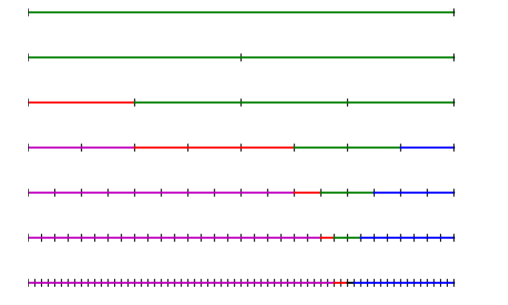
Figure 1: Cluster tree with $\textnormal{{L}}_{n}$ shown in black, the minimal admissible cover $\mathcal{M}(\textnormal{{L}}_{n})$ in red and the other active clusters in green. The blue clusters are not yet active and the magenta clusters are no longer active.

For each cluster $\textnormal{{C}}\in\mathcal{T}$, either there is no $n$ such that $\textnormal{{C}}\in\mathcal{M}(\textnormal{{L}}_{n})$, or else there is a unique smallest $n=n_{\min}(\textnormal{{C}})$ such that $\textnormal{{C}}\in\mathcal{M}(\textnormal{{L}}_{n})$. Moreover, if $\textnormal{{C}}\notin\mathcal{M}(\textnormal{{L}}_{n})$ for some $n>n_{\min}(\textnormal{{C}})$, then an ancestor of C must belong to $\mathcal{M}(\textnormal{{L}}_{n})$ and we have $\textnormal{{C}}\notin\mathcal{M}(\textnormal{{L}}_{n^{\prime}})$ for every $n^{\prime}>n$. Hence, there is also a unique $n=n_{\max}(\textnormal{{C}})$ such that

$$\textnormal{{C}}\in\mathcal{M}(\textnormal{{L}}_{n})\quad\text{if and only if}\quad n_{\min}(\textnormal{{C}})\leq n\leq n_{\max}(\textnormal{{C}}),$$

so, if C is not a leaf, the sums

$$\Psi(\textnormal{{C}},\tilde{U})=\Psi(\textnormal{{C}})=[\Psi_{1}(\textnormal{{C}}),\Psi_{2}(\textnormal{{C}}),\ldots,\Psi_{r}(\textnormal{{C}})]$$

contribute to the far-field sum $\widetilde{\Sigma}_{n}(\textnormal{{C}},\tilde{U})$ if and only if $n_{\min}(\textnormal{{C}})\leq n\leq n_{\max}(\textnormal{{C}})$. We can therefore deallocate the $O(rM)$ memory locations used to store $\Psi(\textnormal{{C}})$ once $\tilde{U}^{n}$ has been computed for $n=n_{\max}(\textnormal{{C}})$.

For each $n$, define a subtree

$$\mathcal{T}_{n}=\{\,\textnormal{{C}}\in\mathcal{T}\setminus\mathcal{L}:\text{$\bigcup\textnormal{{C}}$ intersects $I_{n}$}\,\},$$

so that $\Psi_{p}(\textnormal{{C}},\tilde{U})$ includes a term in $\tilde{U}^{n}$ if and only if $\textnormal{{C}}\in\mathcal{T}_{n}$. In Algorithm 6.1, after computing $\tilde{U}^{n}$ we update all far-field sums $\Psi_{p}(\textnormal{{C}})$ with $\textnormal{{C}}\in\mathcal{T}_{n}$, so that $\tilde{U}^{n}$ is subsequently needed only for computing near-field sums. In this way, we can deallocate the $O(NQ^{-G}M)$ memory locations used to store $U^{j}$ for $I_{j}\in\textnormal{{L}}$ once $\tilde{U}^{n}$ has been computed for $n=n_{\max}(\textnormal{{L}})$. Algorithm 6.2 defines a recursive procedure $\textsl{free}(\textnormal{{C}},V)$ that deallocates the memory associated with the children of C, and with their descendants if not already deallocated.

Algorithm 6.1 Time stepping and memory management.

  for $n=1$ to $N$ do

     Find $\mathcal{M}(\textnormal{{L}}_{n})$ using Algorithm 4.1

     for all $\textnormal{{C}}\in\mathcal{M}(\textnormal{{L}}_{n})\setminus\mathcal{L}$ do

        for all $\textnormal{{C}}^{\prime}$ a child of C do

           $\textsl{free}(\textnormal{{C}}^{\prime},\tilde{U})$

        end for

     end for

     Compute $\widetilde{\mathcal{B}}^{n}\tilde{U}$ using (22)

     Allocate $\tilde{U}^{n}$ and solve (13)

     Write $\tilde{U}^{n}$ to disk

     for all $\textnormal{{C}}\in\mathcal{T}_{n}$ do

        if $\Psi(\textnormal{{C}})$ is not allocated then

           Allocate $\Psi(\textnormal{{C}})$ and initialize to 0.

        end if

        for all $p\in\{1,2,\ldots,r\}$ do

           $\Psi_{p}(\textnormal{{C}})=\Psi_{p}(\textnormal{{C}})+\psi_{pn}\tilde{U}^{n}$

        end for

     end for

  end for

Algorithm 6.2 $\textsl{free}(\textnormal{{C}},V)$

  if $\textnormal{{C}}\in\mathcal{L}$ then

     for all $I_{j}\in\textnormal{{C}}$ do

        Deallocate $V^{j}$

     end for

  else if $\Psi(\textnormal{{C}})$ is allocated then

     for all $\textnormal{{C}}^{\prime}$ a child of C do

        $\textsl{free}(\textnormal{{C}}^{\prime},V)$

     end for

     Deallocate $\Psi(\textnormal{{C}})$

  end if

Theorem 6.1.

The number of active memory locations used during the execution of Algorithm 6.1 is never more than $O(r\eta^{-1}QGM)$.

Proof.

Suppose that the memory associated with C is active during the $n$th time step, and that $\bigcup\textnormal{{C}}=(a,b]$ and $\bigcup\textnormal{{L}}_{n}=(c,d]$. (So in Figure 1, C is green or red or black.) If $\operatorname{Gen}(\textnormal{{C}})=\ell$, then by Lemma 5.2,

$$c-(1+\eta^{-1})\Lambda TQ^{-\ell+1}<a<b\leq d+\Lambda TQ^{-\ell},$$

and since $d-c=\operatorname{Len}(\textnormal{{L}}_{n})\leq\Lambda TQ^{-G}$ and $\operatorname{Len}(\textnormal{{C}})\geq\lambda TQ^{-}\ell$, we see that the number of such clusters is at most

$$\frac{(d-c)+\Lambda TQ^{-\ell}[1+(1+\eta^{-1})Q]}{\lambda TQ^{-\ell}} \leq\frac{\Lambda}{\lambda}\Bigl{(}Q^{\ell-G}+1+(1+\eta^{-1})Q\Bigr{)}$$

$$\leq\frac{\Lambda}{\lambda}(1+\eta^{-1})(Q+1).$$

Storing $\Psi_{p}(\textnormal{{C}},\tilde{U})$ requires $rM$ memory locations, so the desired estimate follows after adding the contributions for $1\leq\ell\leq G$. ∎

Since $G\leq P=\log_{Q}N$, Theorem 6.1 justifies the claim in the Introduction that the memory requirements are proportional to $M\log N$. Theorems 5.3 and 6.1 show that — for a given choice of $M$ and $N$ and a given cluster tree — the computational cost, both with respect to the number of operations and to the number of active memory locations, is proportional to $r/\eta$. At the same time, by Theorem 4.3, to achieve the desired accuracy we must ensure that $(r+1)(\eta/2)^{r}$ is sufficiently small. The next result shows the relation between $r$ and $\eta$ that is optimal in the sense of achieving a given accuracy for the least computational cost.

Proposition 6.2.

For a given $\delta>0$, the ratio $r/\eta$ is minimised subject to the constraint $(r+1)(\eta/2)^{r}=\delta$ by choosing

$$\eta=2\exp\biggl{(}-\frac{r+2}{r+1}\biggr{)}=2\biggl{(}\frac{\delta}{r+1}\biggr{)}^{1/r}.$$ (25)

Proof.

Introducing the Lagrangian $L=r\eta^{-1}+\mu(r+1)(\eta/2)^{r}$, we obtain the necessary conditions

$$\eta^{-1}+\mu(\eta/2)^{r}[1+(1+r)\log(\eta/2)]=0\quad\text{and}\quad-r\eta^{-2}+\mu(r+1)r\eta^{r-1}2^{-r}=0,$$

so $\mu(\eta/2)^{r}=\eta^{-1}/(r+1)$ and $r+2+(r+1)\log(\eta/2)=0$. ∎

Thus, we should choose successive values of $r$ until the second inequality in (23) holds, with $\eta$ given by (25). Since $\eta^{-1}\leq e^{2}/2$, the computational cost is then proportional to $r$.

7 Numerical example

	Slow	Fast
$r$	—	4	5	6
$\eta$	—	0.6024	0.6228	0.6378
Error	0.129E-03	0.136E-02	0.129E-03	0.129E-03
Setup	049.6 s	00.57 s	00.57 s	00.62 s
RHS	910.9 s	15.45 s	17.68 s	20.55 s
Solver	007.2 s	06.96 s	06.84 s	06.68 s
Total	967.7 s	22.97 s	25.10 s	27.85 s

Table 1: Performance of slow and fast methods with $N=16000$ time steps and $M=6241$ spatial degrees of freedom.

Consider a simple test problem in $d=2$ spatial dimensions, with $\nu=1/2$, $T=6$, $\Omega=(0,1)\times(0,1)$ and homogeneous Dirichlet boundary conditions (2). We take $K=1/(2\pi^{2})$ so that the smallest eigenvalue of the elliptic operator $Au=-\nabla\cdot(K\nabla u)$ is $\lambda_{11}=1$. We choose the initial data and source term

$$u_{0}=\varphi_{11}\quad\text{and}\quad f(t)=(1+\sin\pi t)\varphi_{11},$$

where $\varphi_{11}(x)=(\sin\pi x_{1})(\sin\pi x_{2})$ is an eigenfunction of $A$ with eigenvalue $\lambda_{11}$. The exact solution of (1) then has the separable form $u(x,t)=u_{11}(t)\varphi_{11}(x)$, and we can compute the time-dependent factor $u_{11}(t)$ to high accuracy by applying Gauss quadrature to an integral representation [6, Section 6]. Moreover, the regularity estimates (4) hold with $\sigma=1$, so by (5) the $L_{2}$-error in $U^{n}$ is of order $(k+h^{2})\lg(t_{n}/t_{1})$.

Table 1 shows some results of computations performed using a single-threaded Fortran code running on a desktop PC with an Intel Core-i7 860 processor (2.80GHz) and 8GB of RAM. In all cases the spatial discretization used bilinear finite elements on a uniform $80\times 80$ rectangular mesh, so the number of degrees of freedom was $M=79^{2}=6241$. We solved the linear system (6) using fast sine transforms. Taking $N=16000$ time steps, we first computed the (slow) DG solution $U$ and then the perturbed (fast) solution $\tilde{U}$ for $r=4$, 5, 6 choosing $\eta$ as in Proposition 6.2. The table shows the maximum nodal error $\max_{1\leq n\leq N,1\leq m\leq M}|U^{n}_{m}-u(x_{m},t_{n})|$, and also the CPU times in seconds, broken down into three parts. The setup phase covers computing the $\beta_{nj}$ or $\tilde{\beta}_{nj}$, and for the fast method the cost of constructing the cluster tree and admissible covers. The RHS phase covers the computation of the right-hand side of (6), and the solver phase is the total CPU time used by the elliptic solver.

The cluster tree was $(Q,G)$-uniform for $Q=2$ and $G=10$, so there were $2^{G}=1024$ leaves. We see from the table that if $r=5$ then the fast summation algorithm evaluates the right-hand side (RHS) in 17.7 seconds, compared to 911 seconds for a direct evaluation, while maintaining the accuracy of the DG solution.

Appendix A A lower bound

For any real-valued, piecewise-constant $V$,

$$\sum_{n=1}^{N}k_{n}(\bar{\mathcal{B}}^{n}V)V^{n}=\int_{0}^{T}\mathcal{B}V(t)V(t)\,dt\quad\text{and}\quad\sum_{n=1}^{N}k_{n}(V^{n})^{2}=\int_{0}^{T}V(t)^{2}\,dt,$$

so the next theorem shows that (15) holds.

Theorem A.1.

If $v:[0,T]\to\mathbb{R}$ is piecewise $C^{1}$ then

$$\int_{0}^{T}\mathcal{B}v(t)v(t)\,dt\geq\rho_{\nu}T^{\nu-1}\int_{0}^{T}v(t)^{2}\,dt,$$

where

$$\rho_{\nu}=\pi^{1-\nu}\,\frac{(1-\nu)^{1-\nu}}{(2-\nu)^{2-\nu}}\,\sin(\tfrac{1}{2}\pi\nu).$$ (26)

Proof.

The assumption that $v$ is piecewise $C^{1}$ ensures $\mathcal{B}v$ is continuous except for weak singularities at the breakpoints of $v$. Using the substitution $t=\tau T$ for $0<\tau<1$, we see that it suffices to deal with the case $T=1$. Denote the Laplace transform of $u$ by

$$\hat{u}(z)=\int_{0}^{\infty}e^{-zt}u(t)\,dt\quad\text{for $\Re z\geq 0$,}$$

and observe that, because $\hat{\omega}_{\nu}(z)=z^{-\nu}$, if we extend $v$ by zero outside the interval $[0,1]$, then

$$\widehat{\mathcal{B}v}(z)=z\,\hat{\omega}_{\nu}(z)\hat{v}(z)=z^{1-\nu}\hat{v}(z).$$

Applying the Plancherel Theorem, and noting that $\overline{\hat{v}(z)}=\hat{v}(\bar{z})$ because $v$ is real-valued, we have

$$\int_{0}^{\infty}u(t)v(t)\,dt=\frac{1}{2\pi}\int_{-\infty}^{\infty}\hat{u}(iy)\hat{v}(-iy)\,dy.$$

In particular,

$$\int_{0}^{1}v(t)^{2}\,dt=\frac{1}{\pi}\int_{0}^{\infty}|\hat{v}(iy)|^{2}\,dy$$ (27)

and

$$\int_{0}^{1}\mathcal{B}v(t)v(t)\,dt =\int_{0}^{\infty}\mathcal{B}v(t)v(t)\,dt=\frac{1}{2\pi}\int_{-\infty}^{\infty}(iy)^{1-\nu}\hat{v}(iy)\hat{v}(-iy)\,dy$$ (28)

$$=\frac{\sin\tfrac{1}{2}\pi\nu}{\pi}\int_{0}^{\infty}y^{1-\nu}|\hat{v}(iy)|^{2}\,dy.$$

The estimate

$$|\hat{v}(iy)|^{2}\leq\biggl{|}\int_{0}^{1}e^{-iyt}v(t)\,dt\biggr{|}^{2}\leq\int_{0}^{1}v(t)^{2}\,dt$$

implies that, for any $\epsilon>0$,

$$\int_{0}^{\epsilon}|\hat{v}(iy)|^{2}\,dy\leq\epsilon\int_{0}^{1}v(t)^{2}\,dt,$$

and therefore by (27),

$$\int_{0}^{1}v(t)^{2}\,dt\leq\frac{\epsilon}{\pi}\int_{0}^{1}v(t)^{2}\,dt+\frac{1}{\pi}\int_{\epsilon}^{\infty}|\hat{v}(iy)|^{2}\,dy.$$

Thus, for $0<\epsilon<\pi$,

$$\biggl{(}1-\frac{\epsilon}{\pi}\biggr{)}\int_{0}^{1}v(t)^{2}\,dy\leq\frac{1}{\pi}\int_{\epsilon}^{\infty}(y/\epsilon)^{1-\nu}|\hat{v}(iy)|^{2}\,dy\leq\frac{\epsilon^{\nu-1}}{\pi}\int_{0}^{\infty}y^{1-\nu}|\hat{v}(iy)|^{2}\,dy,$$

which, in combination with (28), implies that the desired inequality holds with

$$\rho_{\nu}=\epsilon^{1-\nu}(\pi-\epsilon)\,\frac{\sin\tfrac{1}{2}\pi\nu}{\pi}.$$

The choice $\epsilon=\pi(1-\nu)/(2-\nu)$ maximises $\rho_{\nu}$ and gives the formula (26). ∎

Appendix B Computing the weights

Since the diagonal weights present no difficulty, we assume throughout this appendix that $1\leq j\leq n-1$. Denoting the distance between the centres of $I_{j}$ and $I_{n}$ by $\Delta_{nj}=t_{n-1/2}-t_{j-1/2}$, we see from (17) that

$$\beta_{nj}=-\int_{-k_{j}/2}^{k_{j}/2}\int_{-k_{n}/2}^{k_{n}/2}\omega_{\nu-1}(\Delta_{nj}+t+s)\,dt\,ds$$

and so

$$\beta_{nj}=-\int_{-k_{j}/2}^{k_{j}/2}B_{\nu-1}(\Delta_{nj}+s,k_{n})\,ds=-\int_{-k_{n}/2}^{k_{n}/2}B_{\nu-1}(\Delta_{nj}+t,k_{j})\,dt.$$ (29)

Although we can easily evaluate these integrals analytically, the resulting expressions are susceptible to loss of precision when $k_{j}$ and $k_{n}$ are small compared to $\Delta_{nj}$.

Consider the problem of computing

$$B_{\mu}(t,k)=\omega_{1+\mu}(t+\tfrac{1}{2}k)-\omega_{1+\mu}(t-\tfrac{1}{2}k)$$

when $k$ is small compared to $t$, so that we have a difference of nearly equal numbers. The C99 standard library provides the functions $\texttt{expm1}(x)$ and $\texttt{log1p}(x)$ that approximate $e^{x}-1$ and $\log(1+x)$ accurately even when $x$ is close to zero, so we can avoid the loss of precision by noting that

$$B_{\mu}(t,k)=\omega_{1+\mu}(t+\tfrac{1}{2}k)D_{\mu}\biggl{(}\frac{k}{t+\tfrac{1}{2}k}\biggr{)}\quad\text{where $D_{\mu}(x)=1-(1-x)^{\mu}$,}$$ (30)

and evaluating $D_{\mu}(x)$ as $-\texttt{expm1}\bigl{(}\mu\,\texttt{log1p}(-x)\bigr{)}$.

However, even though we can compute $B_{\mu}(t)$ accurately, we still face the problem that

$$\beta_{nj}=B_{\nu}(\Delta_{nj}-\tfrac{1}{2}k_{j},k_{n})-B_{\nu}(\Delta_{nj}+\tfrac{1}{2}k_{j},k_{n})$$ (31)

is again a difference of nearly equal numbers, as is the alternative formula

$$\beta_{nj}=B_{\nu}(\Delta_{nj}-\tfrac{1}{2}k_{n},k_{j})-B_{\nu}(\Delta_{nj}+\tfrac{1}{2}k_{n},k_{j}),$$

or equivalently

$$\beta_{nj} =\omega_{1+\nu}(t_{n}-t_{j})D_{\nu}\biggl{(}\frac{k_{n}}{t_{n}-t_{j}}\biggr{)}-\omega_{1+\nu}(t_{n}-t_{j-1})D_{\nu}\biggl{(}\frac{k_{n}}{t_{n}-t_{j-1}}\biggr{)}$$

$$=\omega_{1+\nu}(t_{n-1}-t_{j-1})D_{\nu}\biggl{(}\frac{k_{j}}{t_{n-1}-t_{j-1}}\biggr{)}-\omega_{1+\nu}(t_{n}-t_{j-1})D_{\nu}\biggl{(}\frac{k_{j}}{t_{n}-t_{j-1}}\biggr{)}.$$

When $k_{j}$ is small compared to $\Delta_{nj}$, the following sum gives a more accurate value for the weight $\beta_{nj}$.

Theorem B.1.

If $1\leq j\leq n-1$, then there exists $t_{nj}^{*}\in I_{j}$ such that

$$\beta_{nj}=-\sum_{p=0}^{r-1}\frac{B_{\nu-2p-1}(\Delta_{nj},k_{n})}{(2p+1)!2^{2p}}\,k_{j}^{2p+1}-\frac{B_{\nu-2r-1,j}(t_{n-1/2}-t_{nj}^{*},k_{n})}{(2r+1)!2^{2r}}\,k_{j}^{2r+1}.$$

Proof.

We use the first integral representation in (29). The Taylor expansion

$$B_{\nu-1}(\Delta_{nj}+s,k_{n})=\sum_{p=0}^{2r-1}B_{\nu-1-p}(\Delta_{nj},k_{n})\,\frac{s^{p}}{p!}\\ +\int_{0}^{s}\frac{(s-t)^{2r-1}}{(2r-1)!}\,B_{\nu-1-2r}(\Delta_{nj}+t,k_{n})\,dt$$

implies that

$$\int_{-\tfrac{1}{2}k_{j}}^{\tfrac{1}{2}k_{j}}B_{\nu-1}(\Delta_{nj}+s,k_{n})\,ds=\sum_{p=0}^{r-1}B_{\nu-1-2p}(\Delta_{nj},k_{n})\frac{2(\tfrac{1}{2}k_{j})^{2p+1}}{(2p+1)!}+E_{r},$$

with the error term given by $E_{r}=E_{r}^{+}+E_{r}^{-}$, where

$$E_{r}^{\pm}=\int_{0}^{\tfrac{1}{2}k_{j}}\int_{0}^{s}\frac{(s-t)^{2r-1}}{(2r-1)!}B_{\nu-1-2r}(\Delta_{nj}\pm t,k_{n})\,dt\,ds.$$

By the Integral Mean Value Theorem, there exists $\theta_{nj}^{\pm}\in[0,\tfrac{1}{2}k_{j}]$ such that

$$E_{r}^{\pm}=B_{\nu-1-2r}(\Delta_{nj}\pm\theta_{nj}^{\pm},k_{n})\int_{0}^{\tfrac{1}{2}k_{j}}\int_{0}^{s}\frac{(s-t)^{2r-1}}{(2r-1)!}\,dt\,ds\\ =B_{\nu-1-2r}(\Delta_{nj}\pm\theta_{nj}^{\pm},k_{n})\,\frac{(\tfrac{1}{2}k_{j})^{2r+1}}{(2r+1)!}.$$

Since $\Delta_{nj}\pm\theta_{nj}^{\pm}=t_{n-1/2}-(t_{j-1/2}\mp\theta_{nj}^{\pm})$ and $t_{j-1/2}\mp\theta_{nj}^{\pm}\in I_{j}$, by the Intermediate Value Theorem there exists $t_{nj}^{*}\in I_{j}$ such that

$$B_{\nu-1-2r}(\Delta_{nj}+\theta_{nj}^{+},k_{n})+B_{\nu-1-2r}(\Delta_{nj}-\theta_{nj}^{-},k_{n})=2B_{\nu-1-2r}(t_{n-1/2}-t_{nj}^{*},k_{n}).$$

∎

By starting from the second integral representation in (29), we obtain an expansion in odd powers of $k_{n}$, instead of $k_{j}$. For practical meshes, we generally have $k_{j}\leq k_{n}$, so the series in the theorem will be preferable.

To determine the speed of convergence of the series, denote the $p$th term by

$$b_{p}=-\frac{B_{\nu-2p-1}(\Delta_{nj},k_{n})}{(2p+1)!2^{2p}}\,k_{j}^{2p+1},$$

and note that since $D_{-\mu}(x)=-D_{\mu}(x)/(1-x)^{\mu}$,

$$-B_{\nu-2p-1}(\Delta_{nj},k_{n})=\omega_{\nu-2p}(\Delta_{nj}+\tfrac{1}{2}k_{n})\frac{D_{2p+1-\nu}(x)}{(1-x)^{2p+1-\nu}}\quad\text{for $x=\frac{k_{n}}{\Delta_{nj}+\tfrac{1}{2}k_{n}}$.}$$

We find that the ratio of successive terms is

$$\frac{b_{p+1}}{b_{p}}=\frac{1}{4}\,\frac{2p+2-\nu}{2p+3}\,\frac{2p+1-\nu}{2p+2}\,\frac{D_{2p+3-\nu}(x)}{D_{2p+1-\nu}(x)}\biggl{(}\frac{k_{j}}{\Delta_{nj}-\tfrac{1}{2}k_{n}}\biggr{)}^{2},$$

and, since $D_{\mu}(x)\to 1$ as $\mu\to\infty$ for $0<x<1$,

$$\lim_{p\to\infty}\frac{b_{p+1}}{b_{p}}=\biggl{(}\frac{k_{j}}{2\Delta_{nj}-k_{n}}\biggr{)}^{2}.$$

For instance, in the case of a uniform grid $t_{n}=nk$, this limiting ratio is $[2(n-j)-1]^{-2}$, giving acceptable convergence for $j\leq n-2$. If $j=n-1$, then the limiting ratio is $k_{n-1}/(k_{n-1}+k_{n})$, so the convergence is relatively slow. We see from (31) that

$$\beta_{n,n-1} =\omega_{1+\nu}(k_{n})+\omega_{1+\nu}(k_{n-1})-\omega_{1+\nu}(k_{n}+k_{n-1})$$

$$=\omega_{1+\nu}(k_{n})\bigl{[}1+x^{\nu}-(1+x)^{\nu}\bigr{]},\quad\text{for $x=k_{n-1}/k_{n}$,}$$

and from symmetry we may assume $k_{n-1}\leq k_{n}$ and thus $0<x\leq 1$. To evaluate the difference in square brackets, we write

$$(1+x)^{\nu}=1+y^{\nu}\quad\text{where}\quad y=\exp\biggl{(}\frac{\log[(1+x)^{\nu}-1]}{\nu}\biggr{)}$$

computing $(1+x)^{\nu}-1$ as $\texttt{expm1}\bigl{(}\nu\,\texttt{log1p}(x)\bigr{)}$. In this way,

$$1+x^{\nu}-(1+x)^{\nu}=x^{\nu}-y^{\nu}=y^{\nu}\bigl{[}(x/y)^{\nu}-1\bigr{]},$$

and we compute $(x/y)^{\nu}-1$ as $\texttt{expm1}[\nu\log(x/y)]$.

We remark that in the special case $\nu=1/2$ one can evaluate $\beta_{nj}$ more easily. Firstly,

$$B_{1/2}(t,k)=\frac{1}{\Gamma(3/2)}\,\frac{k}{\sqrt{t+\tfrac{1}{2}k}+\sqrt{t-\tfrac{1}{2}k}},$$

and if we write $R_{*\diamond}=\sqrt{\Delta_{nj}*\tfrac{1}{2}k_{j}\diamond\tfrac{1}{2}k_{n}}$ for $*$, $\diamond\in\{+,-\}$, then

$$\beta_{nj} =B_{1/2}(\Delta_{nj}-\tfrac{1}{2}k_{j},k_{n})-B_{1/2}(\Delta_{nj}+\tfrac{1}{2}k_{j},k_{n})$$

$$=\frac{k_{n}}{\Gamma(3/2)}\,\biggl{(}\frac{1}{R_{-+}+R_{--}}-\frac{1}{R_{++}+R_{+-}}\biggr{)}$$

$$=\frac{k_{n}}{\Gamma(3/2)}\,\frac{(R_{++}-R_{-+})+(R_{+-}-R_{--})}{(R_{-+}+R_{--})(R_{++}+R_{+-})}$$

$$=\frac{k_{n}k_{j}}{\Gamma(3/2)}\,\frac{1}{(R_{-+}+R_{--})(R_{++}+R_{+-})}\biggl{(}\frac{1}{R_{++}+R_{-+}}+\frac{1}{R_{+-}+R_{--}}\biggr{)}.$$

Appendix C Computing the Taylor approximations

Recall from Theorem 3.1 that

$$\phi_{pn}=(-1)^{p}B_{\nu-p}(t_{n-1/2}-\bar{s},k_{n})$$

so (30) gives

$$\phi_{pn}=(-1)^{p}\omega_{\nu-p+1}(t_{n}-\bar{s})D_{\nu-p}(x)\quad\text{where $x=\dfrac{k_{n}}{t_{n}-\bar{s}}$.}$$

Since $D_{\nu-p}(x)=-(1-x)^{\nu-p}D_{p-\nu}(x)$ and $1-x=(t_{n-1}-\bar{s})/(t_{n}-\bar{s})$, we have

$$\phi_{pn}=\kappa_{pn}D_{p-\nu}(x),\quad\text{where}\quad\kappa_{pn}=(-1)^{p+1}\frac{(t_{n-1}-\bar{s})^{\nu-p}}{\Gamma(\nu-p+1)},$$

and the $\kappa_{pn}$ can be computed via the recursion

$$\kappa_{1n}=\frac{(t_{n-1}-\bar{s})^{\nu-1}}{\Gamma(\nu)}\quad\text{and}\quad\kappa_{p+1,n}=\frac{p-\nu}{t_{n-1}-\bar{s}}\,\kappa_{p,n}\quad\text{for $1\leq p\leq r-1$.}$$

Likewise,

$$\psi_{pj} =B_{p}(t_{j-1/2}-\bar{s},k_{j})=\frac{1}{p!}\bigl{[}(t_{j-1/2}-\bar{s}+\tfrac{1}{2}k_{j})^{p}-(t_{j-1/2}-\bar{s}-\tfrac{1}{2}k_{j})^{p}\bigr{]}$$

$$=\frac{k_{j}}{p!}\sum_{q=0}^{p-1}(t_{j}-\bar{s})^{q}(t_{j-1}-\bar{s})^{p-1-q},$$

giving $\psi_{1n}=k_{j}$ and

$$\psi_{p+1,j}=\frac{1}{p+1}\biggl{(}(t_{j-1}-\bar{s})\psi_{pj}+\frac{k_{j}}{p!}\,(t_{j}-\bar{s})^{p}\biggr{)}\quad\text{for $1\leq p\leq r-1$.}$$