Spectroscopic Pulsational Frequency Identification and Mode Determination of $\gamma$ Doradus Star HD 135825

Abstract

We present the mode identification of frequencies found in spectroscopic observations of the $\gamma$ Doradus star HD 135825. Four frequencies were successfully identified: $1.3150$ $\pm$ $0.0003$ d^-1; $0.2902$ $\pm$ $0.0004$ d^-1; $1.4045$ $\pm$ $0.0005$ d^-1; and $1.8829$ $\pm$ $0.0005$ d^-1. These correspond to ($l$, $m$) modes of (1,1), (2,-2), (4,0) and (1,1) respectively. Additional frequencies were found but they were below the signal-to-noise limit of the Fourier spectrum and not suitable for mode identification. The rotational axis inclination and $v$sin$i$ of the star were determined to be $87\degree$ (nearly edge-on) and $39.7$ kms^-1 (moderate for $\gamma$ Doradus stars) respectively. A simultaneous fit of these four modes to the line profile variations in the data gives a reduced $\chi^{2}$ of $12.7$. We confirm, based on the frequencies found, that HD 135825 is a bona fide $\gamma$ Doradus star.

1 Introduction

The pulsation of a star is reflective of its internal structure. Since the interior of a star cannot be directly seen, the analysis of the pulsation is the most advanced way to determine interior properties and dynamics. Because pulsations occur in many different types of stars, in many stages of stellar lifetimes, asteroseismology can be used to further our understanding of stellar evolution.

Asteroseismology is the study of vibrational physics in stars, specifically pulsational behaviour in order to derive interior structure properties. The characteristics of pulsation are described by the “quantum numbers” $n$, $l$ and $m$. The radial order, $n$, describes the number of interior nodal shells, $l$ gives the number of nodal lines on the stellar surface and the azimuthal number, $m$, defines the number of nodal lines that intersect the pole.

By analysing the non-radial pulsations and determining the spherical harmonic pulsation modes, we obtain asteroseismic information about the deep interior regions of stars. Non-radial pulsations are classified by the restoring force of the motion: gravity (g-mode) or pressure (p-mode). Gravity-mode pulsations propagate as deep as the convective core interface making them ideal probes of core physics. The detailed frequency spectrum of excited modes places severe constraints on the physical conditions within the regions where these modes propagate. Successful mode identifications can be found in Aerts et al. (2004), Zima et al. (2006) and Böhm et al. (2009) for various types of pulsating star.

The study presented here focuses on one g-mode pulsator, the $\gamma$ Doradus candidate star HD 135825. The defining feature of the $\gamma$ Dor class is the presence of high-order non-radial g-mode pulsations in an A-F type star that is on or near the main sequence (see Kaye et al. 1999 and Kaye 2007, Pollard 2009 for reviews). Thus these stars are slightly hotter and slightly larger than the Sun. A typical feature of the $\gamma$ Dor class is the presence of multiple g-mode pulsations at frequencies lower than the fundamental radial mode . Observed g-mode frequencies generally fall between 0.3 - 3.3 d^-1, although the observed frequencies are dependent on the stellar rotation and direction of the travelling wave. The pulsation frequency range for $\gamma$ Dor stars is similar to the g-mode pulsators of the Slowly Pulsating B (SPB) class, so an estimate of the T_eff or spectral class is required in order to distinguish between these classes. Presently there are less than 100 bright bona fide $\gamma$ Dor stars (see list in Henry et al. 2011) with a further 100 candidates thus far reported by Kepler (Grigahcène et al., 2010; Uytterhoeven et al., 2011).

The $\gamma$ Dor pulsators reside in that part of the Hertzsprung-Russell diagram between the classical instability strip and the solar instability region. Thus they border the regions of the $\delta$ Scuti (p-mode) pulsators and the solar-like oscillators. A few hybrid $\gamma$ Dor/$\delta$ Scuti stars have now been studied (e.g. Henry & Fekel 2005, Uytterhoeven et al. 2008) and further candidates proposed and still being discovered by Kepler (Uytterhoeven et al., 2011; Balona & Dziembowski, 2011). Early indications show that $\gamma$ Dor/$\delta$ Scuti stars may challenge our understanding of the instability strip (Uytterhoeven et al., 2011).

Solar-like variability is driven in the convective envelope of a star from stochastic excitation and has short frequencies (e.g. the F-type star Procyon has solar-like variability frequencies in the range 300-1400 $\micro$Hz, equivalent to 26-121 d^-1, Bedding et al. 2010). Solar-like oscillations also exist in stars slightly hotter than the Sun (Michel et al., 2008) and have been discovered in the $\delta$ Scuti star HD 187547 (Antoci et al., 2011). This indicates that the convective envelope operates efficiently in stars up to 2M_⊙. It is possible that in $\gamma$ Dor stars, being located between solar-like stars and $\delta$ Scuti stars in size and temperature, solar-like oscillations may also be present. No solar-like/$\gamma$ Dor hybrids have yet been discovered but it may be possibile for high-resolution satellite photometry to be able to detect the high frequency pulsations.

The multitude of high-order, low-degree g-modes present in $\gamma$ Dor stars give us information about their interior structure and physical conditions. These stars have both a convective envelope and a convective core, in between which a radiative zone exists. Driving occurs by the “flux-blocking mechanism” where convection at the base of the thin convective envelope modulates flux throughput from the core to the stellar atmosphere (Guzik et al., 2000; Dupret et al., 2004). Asteroseismic study of interior structure requires frequencies to be identified and corresponding modes to be fully characterised with ($l$,$m$) values. Mode analysis can also be used to constrain stellar parameters such as inclination (Wright et al., 2011).

High precision photometry has been successful in identifying up to hundreds of frequencies in $\gamma$ Dor stars (see Chapellier et al. (2011) for an example of 840 identified frequencies using the COROT photometric satellite). Photometry is invaluable in the study of $\gamma$ Dor pulsations as it can be used to find such large numbers of frequencies with high precision and also determine the corresponding $l$ values. Spectroscopy has thus far been limited to ground-based observations and the signal-to-noise requirements for study of spectra have meant longer integration times. The benefit of spectroscopic observations is the determination of both $l$ and $m$ values for each pulsational frequency. As such photometric and spectroscopic studies of these stars are complementary. To date only a handful of $\gamma$ Dor stars have spectroscopic mode identifications published with only a few (less than six) frequencies each. The lack of detailed mode identifications has previously limited interior structure studies but it is hoped that identifications such as in this paper can be incorporated and used to refine current stellar models.

A further aspect of interest in $\gamma$ Dor stars is the effect of rotation on pulsation. Current models assume slow rotation with no effect on the pulsational geometry. The Coriolis and centrifugal accelerations become more important with increased rotation. Rotational effects can lead to differential rotation and, in extreme cases, the breakdown of spherical symmetry (Townsend, 2003; Lignières et al., 2006; Reese et al., 2006). It is still not well understood to what extent rotation affects spectroscopic observations. Rotation can further hinder frequency analysis as $\gamma$ Dor stars have rotational periods of the same order as their pulsational periods.

This study focuses on one member, HD 135825, of the $\gamma$ Dor group of stars to identify the frequencies and modes of the g-mode pulsations present and to look for any observational evidence of hybrid pulsation and rotational effects. Section 2 discusses the specific data acquisition and reduction undertaken. The analysis of the spectra follows in Sections 3 and 4. Specifically, Section 3 breaks down each of the frequency analysis processes. Section 4 then discusses the corresponding mode identifications to the frequencies detected. A discussion of results in context follows in Section 5.

2 Observations and data treatment

In total nearly 300 spectra of HD 135825 were collected from the 1-metre McLellan telescope at Mt John University Observatory (MJUO) in Tekapo, New Zealand ($170\degree 27^{\prime}.9$ E, $43\degree 59^{\prime}.2$ S). The observatory is at an elevation of $1029$ m. Spectra were obtained on the fibre-fed High Efficiency and Resolution Canterbury University Large Echelle Spectrograph (HERCULES). HERCULES operates over a wavelength range of 3800-8000 Å (Hearnshaw et al., 2003) and the $4096$x$4096$ pixel CCD installed in 2007 samples the entire free spectral range in one exposure.

Multi-site data has also been taken for this star. A total of 28 spectra were taken at on the Sadiford Cass Echelle Spectrometer on the 2.1 m telescope at McDonald Observatory, USA. In addition 8 spectra were obtained on the SOPHIE spectrograph on the 193cm Telescope at the Observatoire de Haute Provence, and 3 spectra on the McKellar Spectrograph on the 1.2-metre telescope at the Dominion Astrophysical Observatory. In order to incorporate these data a mean line profile with sufficient signal-to-noise for pulsation analysis must be constructed. The small size of the aforementioned datasets did not allow for a reliable mean profile with sufficient phase coverage to be produced. These data were therefore not incorporated in the present analysis.

Data from MJUO were collected over a period of $18$ months from February 2009 to July 2010. These data were reduced using a MATLAB pipeline written by Dr. Duncan Wright. The pipeline performs the basic steps of flat fielding from white-lamp observations, calculating a dispersion solution from thorium-lamp observations and outputting the data into a two-dimensional format. The observations were then processed in a pipeline written specifically for non-radial pulsation analysis. The processing stage corrects for barycentric motion, removes small differences between observations, fits the continuum using a synthetic spectrum, then normalises and merges the orders for each spectroscopic observation.

Each image was then cross-correlated using the delta-function method (Wright et al. (in preparation), building on Wright (2008), Wright et al. (2007)) to create a representative line-profile. The delta-function method relies on the following assumptions of the spectra: spectral lines at different wavelengths have the same shape, lines of different species and different excitation potentials change in the same way as a result of the pulsation and all lines in a spectrum are varying in phase. The first two criteria were shown to hold to a good approximation in Wright (2008) and a check of lines of various equivalent width, species, excitation potential, wavelength and showed them to be varying consistently in phase in a single spectrum for HD 135825.

Time-series analysis and mode identification was done using the FAMIAS software (Zima, 2008), applied as in Zima et al. (2006). This entailed an analysis of the moments (Balona, 1986; Briquet & Aerts, 2003) and pixel-by-pixel variations which identified the frequencies in the spectral lines. Specifically, FAMIAS uses the moment definition described in Aerts et al. (1992) and revised in Briquet & Aerts (2003).

The software package SigSpec (Reegen, 2007) was used as a validation of the frequency selection method. SigSpec performs a Fourier analysis of a two-dimensional dataset and selects frequencies based on their spectral significance.

Mode identification was done using the Fourier Parameter Fit method. Developed by Wolfgang Zima (Zima, 2009), this extension of the pixel-by-pixel frequency analysis method uses each identified frequency in the line profile variation and matches this to synthetic spectra with input stellar parameters for various modes until the best fit is obtained.

3 Frequency Analysis

HD 135825 is a relatively faint ($V=7.3$), and hence comparatively understudied, $\gamma$ Dor candidate star. It has a moderate $v$sin$i$ of $38\pm 5$ kms^-1 (De Cat et al., 2006). The star was confirmed multi-periodic in photometry by Eyer et al. (2002) and has an effective temperature of $7050\pm 90$ K and log $g$ of $4.39\pm 0.13$, both from (Bruntt et al., 2008) and spectral type F0 (Kazarovets et al., 1999). A full abundance analysis has been done using high-resolution, broad wavelength range spectra by Bruntt et al. (2008) with a Metallicity $[M/H]=+0.13\pm 0.09$ found. Full abundance results are available in the on-line material. One pulsation period has previously been identified in photometry, $0.76053$ d ($1.31487$ d^-1), from the HIPPARCOS satellite data and one best fitting frequency from classification spectroscopy, $0.63$ d ($1.59$ d^-1), both by De Cat et al. (2006). Note the main period from photometry was also suggested as the main period in De Cat et al. (2006) spectroscopy but was not recoverable due to the limited size of the radial velocity dataset.

Each of the frequency variation tests (moments 0-3 and pixel-by-pixel) was used to construct periodograms for the star. Some methods have higher signal-to-noise and thus improve our ability to extract more frequencies. Amplitudes tabulated in this paper are scaled to ratios of $f_{1}$ to allow comparison between identification methods with differing absolute amplitudes.

Representative line profiles are created by cross-correlating hundreds of spectral lines. These profiles of HD 135825 are shown in Figure 1 and are analysed using the pixel-by-pixel and zeroth to third moments. These tests cover all the independent frequencies. In addition to these tests, the software SigSpec was used to analyse all the two-dimensional data sets (all the moments) and also each individual pixel across the line profile, to confirm the frequencies found and their significance.

The window function of the dataset was calculated to show any periodicities intrinsic to the data sampling. The window function for HD 135825 is plotted in Figure 2. As the dataset is from a single site the one-day aliasing is obvious and this can present a problem in the identification of frequencies. In this analysis, care has been taken to consider all one-day aliases and determine the true frequency.

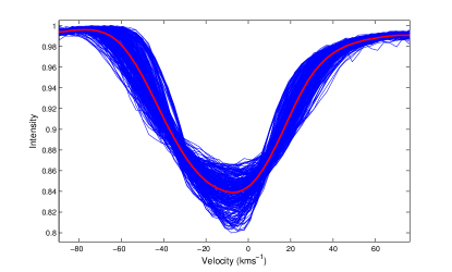
Figure 1: Zero-point profile for the 291 observations of HD 135825 with the mean shown in red. The smooth mean shows that the variations in the profile are well sampled. The line profile data are provided as an on-line file that includes the Modified Julian Date, velocity (on a relative scale) and the intensity at each of the 800 velocity sampling points for each profile.

3.1 Pixel-by-Pixel

The pixel-by-pixel method is an effective tool for examining the frequencies and their fits to the data in two-dimensions as this method performs an analysis of the zero-point line profile by considering the variation of each pixel. The cross-correlated line profile of HD 135825 contained 48 pixels. The pixel-by-pixel technique produced the lowest noise-level in the Fourier spectra. The Fourier spectra for the frequencies ($f_{p}$) are given in Figure 2 and numerical results in Table 1. The phased variations of the zero-point profile are shown in Figure 3(a) and the fits for the four frequencies in Figures 3(b)-3(e). The profiles are smoothed and phased to show the variation over $1.4$ cycles. Where a bin has more than one observation for a particular phase a signal-weighted mean has been used. These plots show the increased matching to the data shape for each successive additional Frequency with the first frequency dominating the shape and the fit.

Table 1 column five shows the amount of variation explained by each frequency combination calculated from the residuals of the fits to the data at each pre-whitening stage. The percentage of the variation explained in the pixel-by-pixel method is generally lower due to several factors. Firstly we are considering the motion of all 48 pixels in the line profile, only about 15 of which are strongly varying (see the amplitude variation profiles as in Figure 9(a)). This means we are considering high and low signal-to noise regions of the line profile. Another effect of considering all pixels in the line profile is the increased precision required to match all the individual pixels. Frequencies, amplitudes and phases must be much more precise for an accurate sum of pixel fits to account for the movement in the line profile. Despite this the Fourier spectra and the reduction of residuals in each pre-whitening stage leaves us confident in the identification of these frequencies. With the fit of four frequencies, some 29$\%$ of the variability in the line profile remains. Much of the remaining variation is likely due to further un-identified frequencies at much lower amplitudes. The signal-to-noise limit of our data (see the red line in Figure 2) restricts the extraction of further frequencies.

Table 1: Frequencies from the pixel-by-pixel analysis of HD 135825 from MJUO.

ID	Frequency	Amplitude	Phase	Cumulative
	($d^{-1}$)	(scaled to $f_{p1}$)		Variation Explained
$f_{p1}$	1.3149	1	0.1033	49%
$f_{p2}$	0.2901	0.4786	0.4199	58%
$f_{p3}$	1.4045	0.4717	0.0368	66%
$f_{p4}$	1.8830	0.3874	0.4058	71%

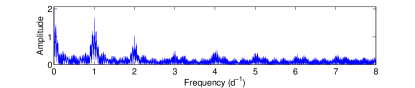
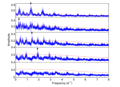
Figure 2: The Fourier spectra showing the amplitude of frequencies detected in the data. 2 Window function for the 291 observations of HD 135825. 2 frequencies found using the pixel-by-pixel technique and successive pre-whitening. The smooth line shows the significance level taken to be the limit of detection.

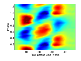
(a) The dataset from MJUO phased to $f_{p1}=1.3149$ d^-1

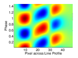
(b) Fit with $f_{p1}$ $(1.3149$d${}^{-1})$

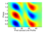
(c) Fit with $f_{p2}$ $(0.2901$d${}^{-1})$

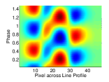
(d) Fit with $f_{p3}$ $(1.4045$d${}^{-1})$

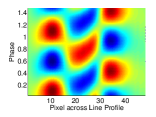
(e) Fit with $f_{p4}$ $(1.8830$d${}^{-1})$

Figure 3: Residual (line profile minus the mean line profile) phased line profiles and fits to the profiles using frequencies (in d^-1) identified with the pixel-by-pixel method. 3(a) Real dataset and 3(b) to 3(e) are the fits to the profiles with the addition of successive frequencies and modes constructed as described in Section 3.8.

3.2 Zeroth Moment (Equivalent Width)

Variations in the equivalent width of the line profile are not expected unless there are significant temperature variations, which makes the analysis much more complex. For HD 135825 only one frequency could be extracted ($1.3147$ d^-1), with a low-amplitude Fourier peak above the noise base. The lack of frequencies in the zeroth moment indicates that there are only small temperature variations centred around the primary frequency and that this star is a good candidate for spectroscopic pulsation analysis.

3.3 First Moment (Radial Velocity)

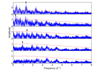
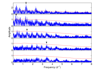
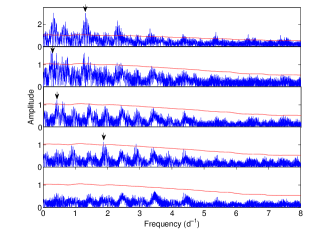
Figure 4: The Fourier spectra showing frequencies found using the $1^{st}$ moment technique with successive pre-whitening. The red line shows the significance level taken to be the limit of detection. Path C was taken to be the best selection of frequencies due to the improvement in the percentage variation and overall frequency amplitude.

The radial velocity measure is a good frequency analysis tool as it is very sensitive to any low-degree modes. First moment results are in good agreement with the results from the pixel-by-pixel search. The Fourier spectra for the frequencies ($f_{a}$) are given in Figures 4-4 and numerical results are shown in Table 2. Due to an uncertainty in the selection of the Fourier peaks, three paths of frequency were selected, A, B and C. The first frequency identified, $0.3122$ d^-1, was a 1-day alias of the main frequency discovered in all other methods. The second peak, $1.3150$ d^-1, had an amplitude almost identical to the first peak and the latter was taken as the true first frequency for analysis. Increasing amplitudes of Fourier spectra is a known effect of higher noise levels in the $0$ to $1$ d^-1 region of the Fourier spectrum, which can push an alias peak of a frequency higher than the real frequency.

There is an ambiguity in the selection of the second and third frequencies. There are two possibilities for the second frequency, either $0.2412$ d^-1 or $0.2902$ d^-1. The $0.2902$ d^-1 frequency was chosen as the other is not consistent with the pixel-by-pixel and SigSpec results. The $0.2902$ d^-1 peak is the second highest peak in the pixel-by-pixel method. Pre-whitening using the $0.2902$ d^-1 frequency removed this peak entirely from the Fourier spectrum in both methods so it was regarded as the best choice for $f_{a2}$. The $0.2412$ d^-1 frequency was still considered in the analysis of Path A. The third frequency is more complex as it first appears as $1.4045$ d^-1 in the pixel-by-pixel method but then a very close frequency, $1.4176$ d^-1, appears using the radial velocity method. It is worth noting that in each of the Fourier spectra the other frequency appears strongly as an additional peak and that choosing the same frequencies as found using the pixel-by-pixel method gives the same frequency set. When $1.8831$ d^-1 was found using this method it had a higher amplitude relative to $f_{a1}$ than $f_{a4}$ given by choosing just the highest peaks. This confirms our choice of Path C.

The radial velocity data is plotted over a selected range of Julian date in Figure 5. This Figure gives an indication of the difference in fit between Path A and Path C.

Even after the removal of four frequencies there still appear to be peaks and aliases in the Fourier spectrum that have amplitudes that are too low to significantly distinguish them from the noise. This could indicate further frequencies are present or that one or more frequencies have been slightly misidentified.

Table 2 shows the amount of variation explained by each frequency combination.

Table 2: Frequencies and amplitudes, relative to $f_{1}a$, $f_{1}b$, $f_{1}c$ identified using the variation of the $1^{st}$, $2^{nd}$ and $3^{rd}$ moments respectively. Note (n) identifies the rank of the frequency peak (high-low) in the case where the highest peak was not chosen. Paths indicated in bold indicate the best choice of frequencies. See text for further explanations of the frequency paths.

First Moment
ID	Frequency (d-1)			Amplitude			Variation Explained
	Path A	Path B	Path C	Path A	Path B	Path C	Path A	Path B	Path C
$f_{a1}$	1.3150			1			53%
$f_{a2}$	0.2412	0.2902(2)		0.5351	0.5278		69%	67%
$f_{a3}$	1.4124	1.4149	0.4040(7)	0.3931	0.4092	0.3388	76%	77%	75%
$f_{a4}$	0.9788	2.4105	1.8831	0.3206	0.3085	0.3761	83%	84%	83%
Second Moment
	Path D	Path E		Path D	Path E		Path D	Path E
$f_{b1}$	1.3149			1			63%
$f_{b2}$	0.4398	0.4043(2)		0.3675	0.3421		70%	70%
$f_{b3}$	1.8829	1.8829		0.3401	0.3519		78%	78%
$f_{b4}$	0.2430	0.7125		0.2454	0.2666		82%	81%
Third Moment
	Path F	Path G	Path H	Path F	Path G	Path H	Path F	Path G	Path H
$f_{c1}$	1.3150			1			58%
$f_{c2}$	0.4126	0.2903(3)		0.4330	0.3948		69%	67%
$f_{c3}$	0.2551	0.4150	0.4040(8)	0.3417	0.3437	0.3142	76%	77%	75%
$f_{c4}$	3.4104	2.4104	1.8831	0.2546	0.2807	0.3429	83%	84%	83%

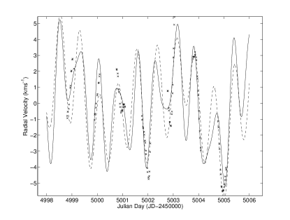
Figure 5: Radial velocity measurements and fits in a section of the HD 135825 data. The crosses show the observed radial velocity and the solid and dashed lines show the fits using Path A and Path C frequencies respectively.

3.4 Second Moment (Variance)

The second moment reflects variations in the width of the line profile and is particularly sensitive to even values of $m$. In general we expect the first and second moments to be complementary and together build a frequency list similar to the pixel-by-pixel findings. In the analysis the first frequency identified was the usual 1.3149 d^-1 and the second frequency that was recovered was $0.4398$ d^-1. Another high peak was seen at the previously identified frequency $0.4043$ d^-1 so both options were studied as a possible frequency path. Frequencies ($f_{b}$) are tabulated for both path D and E in Table 2. Path E found a higher relative amplitude in $f_{b3}$ than Path D. In the $f_{b4}$ spectrum a 1-day alias of the previously identified $0.290$ d^-1 is seen as a high peak in both Fourier spectra. Path E most closely resembles frequencies identified in the pixel-by-pixel method. Table 2 also shows the amount of variation explained by each frequency combination.

3.5 Third Moment (Skewness)

The third moment frequency analysis is known to produce similar frequency sets to the first moment method. It describes the variation in the skewness of the line profile. In this study the third moment also produced the most complicated frequency spectra with three paths (Path F,G and H) or frequency ($f_{c}$) sets being identified (see Table 2). This complication was due to the ambiguity in peaks in the identification of $f_{c2}$ and $f_{c3}$. In this study Path H is chosen as that which identifies the same frequencies as the pixel-by-pixel method and had the highest relative amplitude of $f_{c4}$. The frequency $0.41$ d^-1 was found preferentially in $f_{c2}$ and $f_{c3}$ but vanishes if $0.405$ d^-1 is chosen. The $0.405$ d^-1 is still present in Path F and G as it (or a 1-day alias) occurs as $f_{c4}$ and $f_{c3}$ respectively. This supports the choice of Path H as the best set of frequencies. Table 2 shows the amount of variation explained by each extracted frequency set.

3.6 SigSpec Results

The software package SigSpec (Reegen, 2007) was used to analyse the two-dimensional moments for frequency identification and significance. SigSpec searches the discrete Fourier transform for frequencies and assigns spectral significance. Spectral significance is a measure of false-alarm probability for a given frequency. This probability refers to the likelihood that random noise in the time domain could generate a peak in the Fourier amplitude of similar size as that of the data itself. For example if the risk a noise peak appears at this amplitude is 1:100 000 then the false-alarm probability is 0.00001. This value is equivalent to a spectral significance of 5.0 (Reegen, 2007). The default threshold value for determining frequencies in SigSpec is set at 5.46 (equivalent signal-to-noise = 4) but for the purposes of this analysis we took a much larger threshold of 10. This caution reflects the requirement of precise frequency determination for accurate mode identification. For the three-dimensional pixel-by-pixel dataset, all 48 pixels were individually analysed for frequency identification using SigSpec. The results for each moment are given in Table 3 for all frequencies ($f_{s}$) with spectral significance greater than 10. Many of the frequencies found with significances between 10-15 are not reproduced consistently in other methods of frequency determination and these may not represent true frequencies in the stellar pulsation.

Figure 6 shows the Fourier frequency identification across all 48 pixels and shows the three-bump structure of the line-profile variation and the dominant frequency at $1.315$ d^-1 and 1-day aliases.

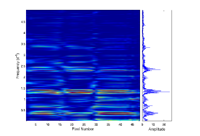
Figure 6: The 2D peridogram (left) showing frequencies found across each pixel (lighter colours for stronger peaks). The peaks at 1.3 $d^{-1}$and 1-day aliases of this frequency are clearly visible. The mean frequencies of the 48 pixels is plotted on the right.

Table 3: Frequencies found using SigSpec above the significance threshold of 10. Frequencies that appear in multiple analysis methods are indicated in bold.

	$1^{st}$ mom	Sig	$2^{nd}$ mom	Sig	$3^{rd}$ mom	Sig
$f_{s1}$	1.3151	33.8	1.3151	40.4	1.3151	37.9
$f_{s2}$	0.2906	19.1	1.4425	13.2	0.4125	16.1
$f_{s3}$	0.4149	17.0	1.8834	15.3	0.2541	14.2
$f_{s4}$	1.9262	15.4	0.2435	11.8	2.4076	12.5
$f_{s5}$	1.4457	15.2			1.9685	12.7
$f_{s6}$	2.5257	11.9			2.4720	10.5
$f_{s7}$	2.1490	11.6			2.1855	12.3
$f_{s8}$					2.6724	10.5
$f_{s9}$					0.0283	11.7
$f_{s10}$					0.2013	11.3

3.7 Frequency Aliases and Combinations

As this analysis produced a significant set of spectroscopic frequencies for a $\gamma$ Dor star, a full study of the Fourier spectra was undertaken. The presence of some combinations for particular frequencies led us to investigate aliasing patterns and possible combinations of true frequencies which may show up in our data. This was done using the frequencies found using the pixel-by-pixel method although other independent frequencies found in the moments were considered.

The $1$ cycle-per-day alias pattern is obvious in our data (Figure 2) due to observations being taken from a single site. Aliasing however does not seem to add significant uncertainties to our frequency identification as the aliases have significantly lower power than the identified frequency. The case where this is most evident is the identification of $f_{p3}$. Mode identification tests of both frequencies showed $1.405$ d^-1 was a better fit to the line profile variation than $0.405$ d^-1. This was not the case for $f_{p2}$ where the $0.290$ d^-1 frequency was found to be a better match to the data, despite being in the longer range of periods for a $\gamma$ Dor star.

Combinations of frequencies are known to occur inherently in the star. The phenomenon has previously been taken into account in the analysis of photometry of $\delta$ Scuti stars such as in Breger et al. (2005). For our set of four identified frequencies a grid search of combinations including addition and subtraction of all frequencies, their multiples and their one-day aliases was undertaken. It was found that there is possibly a link between $f_{p2}$, $f_{p3}$ and $f_{p4}$ as $(f_{p2}+1)-f_{p3}\approx f_{p4}-1$. It was also apparent that the first identified frequency for $f_{3}$ in both the first and third moment is not found indicating it could be an independent frequency. The frequency $f_{2}$ found first in the second moment is half that of identified frequency $f_{p4}$ (excluding one-day aliasing).

3.8 Synthetic Frequency Identification

As an additional test of the validity of the derived frequencies a synthetic data set was constructed using FAMIAS (Zima, 2008). The data used the same time spacings as the real observations and then the four frequencies, their amplitudes, phases and modes (as determined in Section 4) were entered along with the known parameters of the star and representative spectral line. The results for the derivation of the first frequency alone in the data and the first four frequencies together are given in Figures 7 and 8 respectively. All frequencies implanted in the line profiles were able to be extracted, although $f_{p4}$ appeared in the Fourier spectra as a higher peak than $f_{p3}$. The frequencies $2.80$ d^-1 and $1.11$ d^-1 are found as the fifth and sixth frequencies which indicates they are artefact frequencies as only the above four frequencies inserted should be recovered in the Fourier spectrum.

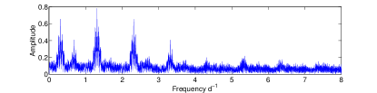
Figure 7: The Fourier spectrum of the synthetic data with only one implanted frequency of $f_{p1}=1.3150$d^-1 at the observational spacing.

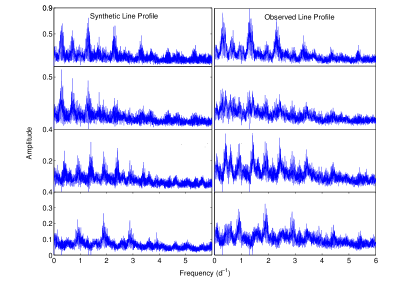
Figure 8: The four Fourier spectra for the identified frequencies in the synthetic reproduction (left) and in the real pixel-by-pixel dataset on the right.

3.9 Frequency Results

A summary of the frequencies found by all methods is presented in Table 4. An error estimate for each frequency ($\sigma(f)$) is given using the definition of Kallinger et al. (2008) who propose:

$$\sigma(f)=\frac{1}{T*\sqrt{sig(a)}},$$ (1)

where T is the time base of observations in days and $sig(a)$ is the spectral significance of the frequency from SigSpec. This equation provides a low uncertainty on our frequencies due to the long time base of observations, but should be regarded as a guide only as the authors feel this uncertainty under-represents the errors present in the frequency identification.

A further least-squares fit of the frequencies to the one-dimensional data was performed to get a second estimate on frequency errors by examination of the 95% confidence bounds. The bounds gave errors on the order of $\pm 0.00002$ d^-1. These errors were disregarded and the previously found SigSpec uncertainties adopted from this point as they are an order of magnitude larger than the confidence fits and it is prudent to remain cautious about the precision of these results.

Four frequencies are confirmed in this study: $1.3150\pm 0.0003$ d^-1, $0.2902\pm 0.0004$ d^-1, $1.4045\pm 0.0005$ d^-1 and $1.8829\pm 0.0005$ d^-1 (Table 4) These are the frequencies found originally in the pixel-by-pixel measurements and confirmed in the $1^{st}$ – $3^{rd}$ moment analysis with uncertainties calculated from significances in the $1^{st}$ moment. Additional frequencies that may be present in the data are $1.44$ d^-1, $0.25$ d^-1 and $1.415$ d^-1. These frequencies had either poor signal-to-noise or misshapen amplitude variation profiles which limited any further mode-identification.

From the identification of multiple frequencies in the 0.3-3 d^-1 range we can confirm HD 135825 is a true $\gamma$ Dor star. After the removal of four frequencies in all the above methods there remained some indication of a periodic signal. It is likely there are further $\gamma$ Dor frequencies present in the data below our detection limit with this dataset. There do not appear to be any higher frequencies suggestive of a $\delta$ Scuti hybrid.

Table 4: Frequencies (in d^-1) identified using pixel-by-pixel (pbp) and $0^{th}$ to $3^{rd}$ moment methods. Note (a) denotes where a one-cycle-per-day alias was found as the highest peak and (#) identifies frequencies which did not have the highest peak but were sequenced according to the number in brackets and chosen as a better result.

	pbp	0th	1st	2nd	3rd	final (d-1)
$f_{1}$	1.3150	1.3147	1.3122 (a)	1.3149	1.3150	1.3150 $\pm$ 0.0003
$f_{2}$	0.2902		0.2902 (2)	0.4043 (2)	0.2903 (3)	0.2902 $\pm$ 0.0004
$f_{3}$	1.4045		0.4039	1.8829	0.4040 (8)	1.4045 $\pm$ 0.0005
$f_{4}$	1.8829		1.8831		1.8831	1.8829 $\pm$ 0.0005

4 Mode Identification

The first calculation performed was a fit to the zero-point profile using the parameters $v$sin$i$, equivalent width and velocity offset. The latter is used to bring the observational data onto a consistent scale. These values were then used to refine future searches in parameter space. To continue with mode identification of the pulsation frequencies, the three Fourier parameters (zero-point, amplitude and phase variations across the cross-correlated line profiles) were calculated. Using the Fourier Parameter Fit Method (Zima, 2009), the modes of each of the final frequencies in Table 4 were found independently, as well as the combination of the four frequencies. This was done using the frequency analysis package in FAMIAS (Zima, 2008). The fits for each mode were performed on the amplitude and phase distributions and a $\chi^{2}$ calculated. The pulsation parameter space that was searched (using a genetic algorithm optimisation to search parameter space) is outlined in Table 5.

Figures 9(a)-9(d) show the Fourier parameters and their fits to the amplitude and phase across the line profile for the four frequencies. Note that FAMIAS sometimes generates phases (see Figures 9(a),9(b),9(d)) that are $\pm$1 cycle ($\pm$2$\pi$) displaced with respect to the observations. The mode fits are best for the even frequencies, $f_{2}$ ($=$0.2902 d^-1; (l,m)$=$(2,-2)) and $f_{4}$ ($=$1.8829 d^-1; (1,1)) that have $\chi^{2}$ $=$ 3.1 and 2.5 respectively, whereas $f_{1}$ ($=$1.3150 d^-1; (1,1)) and $f_{3}$ ($=$1.4045 d^-1; (4,0)) have $\chi^{2}$ of 12.9 and 10.6 respectively. The most significant deviations are in the $f_{3}$ fits where the amplitude and phase are not fitted well, albeit with lower pulsational amplitudes than $f_{1}$ and $f_{2}$.

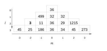
(b) $\chi^{2}$ values for $l=0-3$ for $f_{2}=0.2902$d^-1.
      Best fit value is for ($l,m$) = (2,-2).

(c) $\chi^{2}$ values for $l=0-4$ for $f_{1}=1.4045$d^-1.
      Best fit value is for ($l,m$) = (4,0).

(d) $\chi^{2}$ values for $l=0-3$ for $f_{1}=1.8829$d^-1.
      Best fit value is for ($l,m$) = (1,1).

Figure 10: Lowest $\chi^{2}$ values for each possible ($l,m$) combination for the final identified frequencies. The best fit $\chi^{2}$ is identified in bold.

The final parameters of the fit to each of the modes individually, the $\chi^{2}$ value and stellar parameters are given in Table 6. The mode with the lowest $\chi^{2}$ fit was selected as the best mode. This was an unambiguous selection as there was only one mode for each frequency with a significantly lower $\chi^{2}$. The $\chi^{2}$ of each mode fit to the final frequencies is given in Figures 10(a)-10(d). The individual $\chi^{2}$ values can be used as a guide to the goodness of fit but frequencies with higher amplitudes and small errors have tighter fit constraints. Couple this with the poorly modelled asymmetry in the line profile and the $\chi^{2}$ can be higher than is expected with a good fit such as for $f_{1}$. When all modes were combined for a simultaneous fit a reduced $\chi^{2}$ of $12.7$ was achieved with the stellar variables and line parameters in Table 6. The other best possible fits to the data are shown in Table 7. Although some alternate fits to $f_{3}$ have a similar $\chi^{2}$, the shape of these other fits do not show the four bumps as in the line profile variation. The second and third best fit modes have three and two bumps respectively in the amplitude variation profiles and do not display four distinct changes in the phase and thus we are confident the (4,0) identification is the best match.

The best individual values for the parameters are given by the best fits which are to the second and fourth frequencies. The values for the first frequency also merit consideration given its dominant contribution to the line-profile variation. The range of values found for the inclination of the star show it is an uncertain result of the search, but values between $50\degree-90\degree$ are reasonable and an inclination close to $90\degree$ may explain the number of detected frequencies, as we observe the star edge-on. This means we see the full surface of the star as it rotates. The value for $v$sin$i$ was measured from the line profile to be 38 $\pm$ 5 kms^-1 (De Cat et al., 2006).

Table 5: Stellar parameters used in the mode identification. Fixed values for Teff, [M/H] and log $g$ were taken from Bruntt et al. (2008) and $v$sin$i$ values from De Cat et al. (2006). Values for the other parameters were taken as reasonable limits for $\gamma$ Dor stars.

Property	Fixed Value	Min	Max	Step
Radius(solar units)		1	5	0.1
Mass (solar units)		0.5	5	0.01
Temperature (K)	7050
Metallicity [M/H]	0.13
log $g$	4.39
Inclination ($\degree$)		0	90	1
$v$sin$i$ (kms-1)		30	50	1

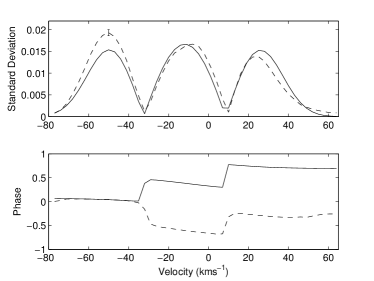
(a) $f_{1}=1.3150$ d^-1 fit with (1,1) mode, $\chi^{2}=12.9$.

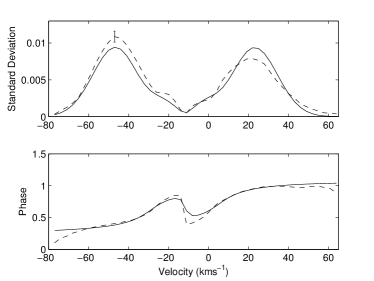
(b) $f_{2}=0.2902$ d^-1 fit with (2,-2) mode, $\chi^{2}=3.1$.

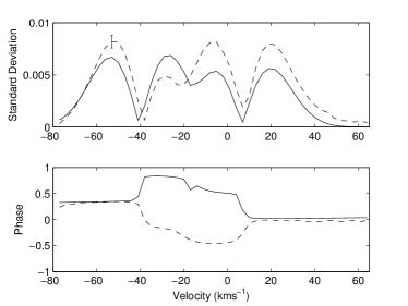
(c) $f_{3}=1.4045$ d^-1 fit with (4,0) mode, $\chi^{2}=10.6$.

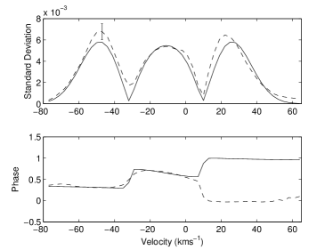
(d) $f_{4}=1.8829$ d^-1 fit with (1,1) mode, $\chi^{2}=2.5$.

Figure 9: Mode identification results. Amplitude variation and phase across the line profile (solid) of the four identified frequencies with the lowest $\chi^{2}$ fits (dashed). A maximum error bar for the fits is given in each amplitude variation plot. Errors on the data and phases are too small to display.

Table 6: Results of mode identification for $f_{1}$ alone, all four frequencies individually after a least-squares fit is applied (lsf), and all four frequencies simultaneously (sim).

freq	Mode ID	$\chi^{2}$	Inclination	Vel. amp	Phase
			($\degree$)	(kms-1)
$f_{1}$	(1,1)	7.6	87	0.78	0.64
$f_{1}$ lsf	(1,1)	12.9	64	0.78	0.64
$f_{2}$ lsf	(2,-2)	3.1	55	0.65	0.43
$f_{3}$ lsf	(4,0)	10.6	88	0.65	0.40
$f_{4}$ lsf	(1,1)	2.5	51	0.65	0.88
$f_{1}$ sim	(1,1)	12.7	87	0.80	0.63
$f_{2}$ sim	(2,-2)			0.50	0.41
$f_{3}$ sim	(4,0)			0.67	0.40
$f_{4}$ sim	(1,1)			0.69	0.91

Table 7: Best fits for modes identified for HD 135825

$f_{1}$	$f_{2}$	$f_{3}$	$f_{4}$	$\chi^{2}$
(1,1)	(2,-2)	(4,0)	(1,1)	10.6
		(1,1)		12.7
		(2,-2)		13.9
		(5,4)		14.9
		(3,-1)		15.5
		(3,-3)		15.6
		(4,3)		15.8

4.1 Rotation and Pulsation Parameters

FAMIAS has a tool to provide a check for the validity of the mode identification method based on the rotational parameters of the star. The stellar rotational parameters of equatorial rotational velocity (v_rot; v_rot = 2$\pi$R$f_{rot}$), rotational period (T_rot), rotational frequency ($f_{rot}$), critical velocity (v_crit) , critical vsini ($v$sin$i_{crit}$) and critical minimum inclination ($i$) are calculated from inputs of mass, radius, $v$sin$i$ and inclination using estimates for mass and radius typical of $\gamma$ Dor stars (1.5 M_⊙ and 1.6 R_⊙) and $v$sin$i$ and inclination from the mode identification (39.7 kms^-1 and 87$\degree$). The results are tabulated below:

vrot	39.75 kms-1
Trot	2.03 d
$f_{rot}$	0.49 d-1
vcrit	423 kms-1
$v$sin$i_{crit}$	423 kms-1
$i_{crit}$	5.4$\degree$

From the above table we can see that HD 135825 is not near the break-up limit of the star and is naturally rotating with a period of around two days. The ratio of horizontal to vertical amplitude of the pulsation ($\kappa$), is calculated using the equation

$$\kappa=\frac{GM}{\omega^{2}R^{3}},$$ (2)

where $G$ is the gravitational constant, $R$ and $M$ are the stellar mass and radius and $\omega$ is the angular frequency. For the various frequencies $\kappa$ was much greater than $1.0$ which indicates low-frequency g-modes as we expect for $\gamma$ Dor stars. We can also use the determined inclination to transform our observed frequencies into the co-rotating frequencies ($f_{co-rot}$) required to model the star ($f_{co-rot}=f_{obs}-mf_{rot}$). These frequencies, along with the horizontal-to-vertical amplitude ratios calculated using Equation 2, are given in Table 8. All of the frequencies lie now in the range accepted for $\gamma$ Dor stars which strengthens our confidence in having obtained correct frequency identifications, particularly for $f_{2}$ which was unusually low. We also show the ratio of the rotational frequency to the co-rotating frequency which can give an indication to the validity of the mode identification models being applied by FAMIAS. In general ratios less than 0.5 are considered to lie well within the parameter space which FAMIAS can produce reliable results, however this is dependent on the value of $m$ considered. Townsend (2003) demonstrated that prograde modes ($m>0$) are distorted less from increasing Coriolis force, increasing the limits of reliability. See Wright et al. (2011) for further discussion.

Note the results obtained in this section must be regarded as approximate as we have estimated the stellar mass and radius.

(a) $\chi^{2}$ values for $l=0-3$ for $f_{1}=1.3150$d^-1.
      Best fit value is for ($l,m$) = (1,1).

Table 8: Stellar rotational frequencies. Final frequencies, their co-rotational values ($f_{co-rot}$), horizontal-to-vertical amplitude ratio ($\kappa$, see equation 2) and ratio of rotational frequency ($f_{rot}$) to each co-rotational frequency.

Frequency	Frequency	$f_{co-rot}$	$\kappa$	$f_{rot}$/$f_{co-rot}$
ID	d-1	d-1
$f_{1}$	1.3150	0.8241	40	0.6
$f_{2}$	0.2902	1.2720	17	0.4
$f_{3}$	1.4045	1.4045	14	0.3
$f_{4}$	1.8829	1.3920	14	0.4

5 Discussion

The dataset in this study provides the largest spectroscopic, and indeed largest observational, dataset for HD 135825 to date. We are now in a position to examine our results in the context of previous work on this star. Multi-periodicy was first confirmed in photometry by Eyer et al. (2002) (Note on page 209 HD 135825 (HIP 74825) is incorrectly written as HD 135828) but no frequencies were published. One pulsation period was identified in HIPPARCOS photometry, $0.76053$ d ($1.31487$ d^-1) (De Cat et al., 2006). In the same paper $17$ spectra were analysed and one period peak identified at $0.63$ d ($1.59$ d^-1), but this was treated with caution due to the limited spectra available at the time. No mode-identification has previously been published. As mentioned above, the $v$sin$i$ value of $39.7$ kms^-1 matches well with previously published of $38\pm 5$ kms^-1 De Cat et al. (2006)

The first frequency extracted in this study matches that found in HIPPARCOS data, but the $1.59$ d^-1 frequency was not found.

The high numbers of single-site data can be used to extract multiple frequencies from a g-mode pulsator. It is worth noting that much of the ambiguity in the path selection and hence frequency identification in the $1^{st}$–$3^{rd}$ moments could be removed using multi-site data. It is also necessary that any multi-site data is acquired such that it covers the phase range of the frequencies independently. Figure 5 shows how multi-site data could distinguish clearly the better frequency fits by providing data points where the fits differ. Despite the increased difficulty in extracting the pulsations from single-site data, the authors are confident that the frequency and mode identifications given in this research are robust, given that similar results are obtained from independent analysis techniques.

We can now begin to remark on the size and quality of spectra required to undertake geometric pulsation analysis in spectroscopy. The dataset produced high signal-to-noise frequencies and clear mode identifications using $291$ high-resolution spectra taken over 18 months. It is clear that this is a demanding standard to study all $\gamma$ Dor stars but the significant increase in precision and ability to successfully identify multiple frequencies warrants this approach. It is noted that not all stars will produce similar results with large datasets. For example, HD 40745 (Maisonneuve et al., 2011) has complicated frequencies and modes even using more than 400 spectra of a comparable quality to this study. Even more spectra (nearly 700 from multiple sites) were obtained by Uytterhoeven et al. (2008) on the star HD 49434 and up to six frequencies were found in each of the spectroscopic methods although only some frequencies were found in multiple methods.

Single-line analysis of the frequencies in HD 135825 produced the same $f_{1}$ in phase for all lines tested. The assumption that all spectral lines move in phase has been found true for all $\gamma$ Dor stars published to date (see Maisonneuve et al. (2011), Wright (2008) for more examples). This demonstrates that these stars are suitable for application of the cross-correlation method and this technique is recommended to obtain sufficiently high signal-to-noise to determine multiple frequencies in spectroscopic data.

As observational asteroseismology of $\gamma$ Dor stars moves beyond the classification phase into producing more individual identifications, it seems likely most stars will require similarly large, or larger datasets as this study. Stars with temperature variations and other periodic structure, such as tidal effects from binaries, will provide further challenges and also require massive datasets.

It is clear that high-precision spectroscopic mode identification is dependent on the availability of high-precision spectral abundance analysis and modelling. The production of the best mode identification is reliant on the availability of T_eff and log $g$ measurements and also benefits from good estimates of stellar masses, radii and inclination. The production of co-rotating frequencies is crucially dependent on precise values of inclination and radius, which are not well constrained in the current mode-identification method.

Even small numbers of full mode-identified frequencies can be used to place constraints on stellar models, particularly on the conditions required to produce such a selection of excited modes. Future work is to take the mode identifications of HD 135825 from this paper and use them in complex theoretical models (e.g. Townsend 2003) to further constrain stellar parameters and to study the extent of the core. This could give us important insights into the evolutionary past and future of the star. Feedback from such models will additionally inform our mode identification methods and lead us ever closer to understanding these information-rich $\gamma$ Dor stars.

6 Acknowledgements

This work was supported by the Marsden Fund.

The authors acknowledge the assistance of staff at Mt John University of Observatory, a research station of the University of Canterbury.

We appreciate the time allocated at other facilities for multi-site campaigns, paticularly the Dominion Astrophysical Observatory, McDonald Observatory and L’Observatoire de Haute Provence.

Gratitude must be extended to the numerous observers who make acquisition of large datasets possible. We thank L.S. Yang Stephenson for observations taken at the DAO.

This research has made use of the SIMBAD astronomical database operated at the CDS in Strasbourg, France.

Mode identification results obtained with the software package FAMIAS developed in the framework of the FP6 European Coordination action HELAS (http://www.helas-eu.org/).

P.L.C. acknowledges the hospitality of the MPA from 2011 May- August that enabled him to devote time to various research projects.

We are thankful to our anonymous referee for helpful comments which improved this manuscript.

References

- Aerts et al. (2004) Aerts C., De Cat P., Handler G., Heiter U., Balona L. A., Krzesinski J., Mathias P., Lehmann H., Ilyin I., De Ridder J., Dreizler S., Bruch A., Traulsen I., Hoffmann A., James D., Romero-Colmenero E., Maas T., et al., 2004, MNRAS, 347, 463
- Aerts et al. (1992) Aerts C., de Pauw M., Waelkens C., 1992, A&A, 266, 294
- Antoci et al. (2011) Antoci V., Handler G., Campante T. L., Thygesen A. O., Moya A., Kallinger T., Stello D., Grigahcène A., Kjeldsen H., Bedding T. R., et al., 2011, NAT, 477, 570
- Balona (1986) Balona L. A., 1986, MNRAS, 219, 111
- Balona & Dziembowski (2011) Balona L. A., Dziembowski W. A., 2011, MNRAS, 417, 591
- Bedding et al. (2010) Bedding T. R., Kjeldsen H., Campante T. L., Appourchaux T., Bonanno A., Chaplin W. J., Garcia R. A., Martić M., Mosser B., Butler R. P., Bruntt H., Kiss L. L., O’Toole S. J., Kambe E., et al., 2010, ApJ, 713, 935
- Böhm et al. (2009) Böhm T., Zima W., Catala C., Alecian E., Pollard K., Wright D., 2009, A&A, 497, 183
- Breger et al. (2005) Breger M., Lenz P., Antoci V., Guggenberger E., Shobbrook R. R., Handler G., Ngwato B., Rodler F., Rodriguez E., López de Coca P., Rolland A., Costa V., 2005, A&A, 435, 955
- Briquet & Aerts (2003) Briquet M., Aerts C., 2003, A&A, 398, 687
- Bruntt et al. (2008) Bruntt H., De Cat P., Aerts C., 2008, A&A, 478, 487
- Chapellier et al. (2011) Chapellier E., Rodríguez E., Auvergne M., Uytterhoeven K., Mathias P., Bouabid M.-P., et al., 2011, A&A, 525, A23
- De Cat et al. (2006) De Cat P., Eyer L., Cuypers J., Aerts C., Vandenbussche B., Uytterhoeven K., Reyniers K., Kolenberg K., Groenewegen M., Raskin G., Maas T., Jankov S., 2006, A&A, 449, 281
- Dupret et al. (2004) Dupret M.-A., Grigahcène A., Garrido R., Gabriel M., Scuflaire R., 2004, AAP, 414, L17
- Eyer et al. (2002) Eyer L., Aerts C., van Loon M., Bouckaert F., Cuypers J., 2002, in C. Sterken & D. W. Kurtz ed., Observational Aspects of Pulsating B- and A Stars Vol. 256 of Astronomical Society of the Pacific Conference Series, The gamma Doradus stars campaign. p. 203
- Grigahcène et al. (2010) Grigahcène A., Antoci V., Balona L., Catanzaro G., Daszyńska-Daszkiewicz J., Guzik J. A., Handler G., Houdek G., Kurtz D. W., Marconi M., Monteiro M. J. P. F. G., et al., 2010, ApJ, 713, L192
- Guzik et al. (2000) Guzik J. A., Kaye A. B., Bradley P. A., Cox A. N., Neuforge C., 2000, ApJ, 542, L57
- Hearnshaw et al. (2003) Hearnshaw J. B., Barnes S. I., Frost N., Kershaw G. M., Graham G., Nankivell G. R., 2003, in S. Ikeuchi, J. Hearnshaw, & T. Hanawa ed., The Proceedings of the IAU 8th Asian-Pacific Regional Meeting, Volume I Vol. 289 of Astronomical Society of the Pacific Conference Series, HERCULES: A High-resolution Spectrograph for Small to Medium-sized Telescopes. pp 11–16
- Henry & Fekel (2005) Henry G. W., Fekel F. C., 2005, AJ, 129, 2026
- Henry et al. (2011) Henry G. W., Fekel F. C., Henry S. M., 2011, AJ, 142, 39
- Kallinger et al. (2008) Kallinger T., Reegen P., Weiss W. W., 2008, A&A, 481, 571
- Kaye (2007) Kaye A. B., 2007, Communications in Asteroseismology, 150, 91
- Kaye et al. (1999) Kaye A. B., Handler G., Krisciunas K., Poretti E., Zerbi F. M., 1999, PASP, 111, 840
- Kazarovets et al. (1999) Kazarovets E. V., Samus N. N., Durlevich O. V., Frolov M. S., Antipin S. V., Kireeva N. N., Pastukhova E. N., 1999, IBVS, 4659, 1
- Lignières et al. (2006) Lignières F., Rieutord M., Reese D., 2006, A&A, 455, 607
- Maisonneuve et al. (2011) Maisonneuve F., Pollard K. R., Cottrell P. L., Wright D. J., De Cat P., Mantegazza L., Kilmartin P. M., Suárez J. C., Rainer M., Poretti E., 2011, MNRAS, 415, 2977
- Michel et al. (2008) Michel E., Baglin A., Auvergne M., Catala C., Samadi R., Baudin F., Appourchaux T., Barban C., Weiss W. W., Berthomieu G., Boumier P., et al., 2008, Science, 322, 558
- Pollard (2009) Pollard K. R., 2009, in J. A. Guzik & P. A. Bradley ed., American Institute of Physics Conference Series Vol. 1170 of American Institute of Physics Conference Series, A Review Of Doradus Variables. pp 455–466
- Reegen (2007) Reegen P., 2007, A&A, 467, 1353
- Reese et al. (2006) Reese D., Lignières F., Rieutord M., 2006, A&A, 455, 621
- Townsend (2003) Townsend R. H. D., 2003, MNRAS, 343, 125
- Uytterhoeven et al. (2008) Uytterhoeven K., Mathias P., Poretti E., Rainer M., Martín-Ruiz S., Rodríguez E.and Amado P. J., Le Contel D., Jankov S., Niemczura E., Pollard K. R., Brunsden E., Paparó M., Costa V., et al., 2008, A&A, 489, 1213
- Uytterhoeven et al. (2011) Uytterhoeven K., Moya A., Grigahcène A., Guzik J. A., Gutiérrez-Soto J., Smalley B., Handler G., Balona L. A., Niemczura E., Fox Machado L., Benatti S., Chapellier E., Tkachenko A., et al., 2011, AAP, 534, A125
- Wright (2008) Wright D. J., 2008, PhD thesis, University of Canterbury
- Wright et al. (2011) Wright D. J., Chené A.-N., De Cat P., Marois C., Mathias P., Macintosh B., Isaacs J., Lehmann H., Hartmann M., 2011, APJL, 728, L20
- Wright et al. (2007) Wright D. J., Pollard K. R., Cottrell P. L., 2007, CoAst, 150, 135
- Zima (2008) Zima W., 2008, CoAst, 157, 387
- Zima (2009) Zima W., 2009, A&A, 497, 827
- Zima et al. (2006) Zima W., Wright D., Bentley J., Cottrell P. L., Heiter U., Mathias P., Poretti E., Lehmann H., Montemayor T. J., Breger M., 2006, A&A, 455, 235