Strong coupling of finite element methods for the Stokes-Darcy problem

Abstract

The aim of this paper is to propose a systematic way to obtain convergent finite element schemes for the Darcy-Stokes flow problem by combining well-known mixed finite elements that are separately convergent for Darcy and Stokes problems. In the approach in which the Darcy problem is set in its natural $\mathbf{H}(\text{div})$ formulation and the Stokes problem is expressed in velocity-pressure form, the transmission condition ensuring global mass conservation becomes essential. As opposed to the strategy that handles weakly this transmission condition through a Lagrange multiplier, we impose here this restriction exactly in the space of global velocity field. Our analysis of the Galerkin discretization of the resulting problem reveals that, if the mixed finite element space used in the Darcy domain admits an $\mathbf{H}(\text{div})$-stable discrete lifting of the normal trace, then it can be combined with any stable Stokes mixed finite element of the same order to deliver a stable global method with quasi-optimal convergence rate. Finally, we present a series of numerical tests confirming our theoretical convergence estimates.

1 Introduction

In this paper we are interested by the mixed finite element approximation of the coupled Darcy-Stokes problem. The Darcy-Stokes coupled system provides a linear model for the simulation of incompressible flows in heterogeneous media. It is governed by the Stokes equations in one part of the domain, while in the other part, the flow is described by a standard second order elliptic equation derived from Darcy’s law and conservation of mass. Proper transmission conditions must also be prescribed on the boundary common to the two media: conservation of mass enforces continuity of the normal velocities at this interface and conservation of momentum enforces the balance of the normal stresses. A further interface condition, supported by empirical evidence and known as the Beavers-Joseph-Saffman condition, must also be taken into account, cf. [2, 20, 16].

The development of suitable numerical methods for the Darcy-Stokes flow interaction has become a subject of increasing interest during the last decade. Discacciati et al. [7] provided the first theoretical study of the problem. The Galerkin scheme discussed in [7] is based on a standard finite element method for second order elliptic problems in the Darcy domain. Motivated by the need of obtaining direct finite element approximations of the Darcy flux, most of the approaches (cf. for instance [18, 3, 10, 17, 12] ) consider now an $\mathbf{H}(\text{div})$-flux conforming formulation in the Darcy domain. Hence, in this case, a mixed variational formulation in the porous media is coupled with the usual velocity-pressure formulation in the Stokes domain. We also point out that other finite element discretization strategies have been considered for this problem. For instance, a discontinuous Galerkin method is described in [19] and a stabilized finite element method is presented in [6].

In the mixed approach, the transmission condition that guaranties the equilibrium of the normal velocities becomes essential. One approach to deal with this constraint consists in enforcing it weakly by means of a Lagrange multiplier representing the trace of the Darcy pressure on the common interface, see for example [18, 10, 12]. One known feature of the finite element discretization of this formulation is that two meshes are required on the transmission boundary satisfying a stability condition between their corresponding mesh sizes, which certainly constitutes a quite cumbersome restriction.

In this paper we are interested in the strong coupling that considers the inclusion of the essential transmission condition directly in the definition of the space to which the Darcy flux and the fluid velocity belong (see (2.9) below). This formulation prevents from introducing a further unknown (the Lagrange multiplier) simplifying by the way the saddle point structure of the problem. Two finite element discretizations have already been proposed for this formulation of the problem. In the first one [17] the authors provide a unified approximation in the whole domain giving rise to a global $\mathbf{H}(\text{div})$-conforming scheme that is nonconforming in the fluid domain. In the second one [3], a mortar discretization that combines the Bernardi-Raugel element and the lowest order Raviart-Thomas element is studied.

Our concern in this paper is to figure out how to combine any of the common mixed finite element methods for Darcy and Stokes problems to end up with a stable scheme for the coupled problem. We consider stable conforming Galerkin schemes in each subdomain and establish the rules under which these schemes can be matched to form a global convergent method. We will see that the only requirement for the viability of such a coupling is the existence of a discrete stable lifting of the normal trace in $\mathbf{H}(\text{div})$. We can prove that such a lifting is available in the bi-dimensional case for the Raviart-Thomas and the Brezzi-Douglas-Marini elements while, in the three-dimensional case, to obtain the same result, we need to assume that the triangulation is quasi-uniform in a neighborhood of the transmission boundary.

The paper is organized as follows. In Section 2 we decribe the governing equations, derive a mixed variational formulation of the problem and show that it is well-posed. Our Galerkin scheme is introduced in Section 3 by means of abstract finite elements spaces in each subdomain. We also establish in this section the conditions guarantying the stability of our approximation method. In Section 4, we discuss the approximation properties of the discrete space for the global velocity field and provide our main convergence result. The key hypotheses providing the convergence of our numerical scheme are discussed in Sections 5 and 6. We show that they are satisfied for the most common mixed finite elements for Darcy and Stokes problems under mild conditions on the family of finite element triangulations. In Section 7 we provide some examples obtained by combining well-known finite elements for the Stokes problem, such as the MINI element and the Bernardi-Raugel element, with the Raviart-Thomas and the Brezzi-Douglas-Marini elements in order to obtain a global scheme for the coupled Darcy-Stokes problem. Finally, in Section 8, we present a set of numerical experiments that confirm the converge rate predicted by the theory of the examples described in the former section.

Notation and background.

Boldface fonts will be used to denote vectors and vector valued functions. Also, if $H$ is a vector space of scalar functions, $\mathbf{H}$ will denote the space of $\mathbb{R}^{d}$ valued functions whose components are in $H$, endowed with the product norm.

Given an integer $m\geq 1$ and a bounded Lipschitz domain $\mathcal{O}\subset\mathbb{R}^{d}$, $(d=2,3)$, we denote by $\|\cdot\|_{H^{m}(\mathcal{O})}$ the norm in the usual Sobolev space $H^{m}(\mathcal{O})$, cf. [1]. For economy of notation, $(\cdot,\cdot)_{\mathcal{O}}$ stands for the inner product in $L^{2}(\mathcal{O})$ and $\|\cdot\|_{\mathcal{O}}$ is the corresponding norm. We recall that $H^{1/2}(\partial\mathcal{O})$ represents the image of $H^{1}(\mathcal{O})$ by the trace operator. Its dual with respect to the pivot space $L^{2}(\partial\mathcal{O})$ is denoted $H^{-1/2}(\partial\mathcal{O})$. If $\Sigma$ is a part of the Lipschitz boundary $\partial\mathcal{O}$, we denote by $H_{00}^{1/2}(\Sigma)$ the space of functions from $H^{1/2}(\Sigma)$ whose extension by zero to the whole $\partial\mathcal{O}$ belongs to $H^{1/2}(\partial\mathcal{O})$. We will consider the dual $H_{00}^{-1/2}(\Sigma)$ of $H_{00}^{1/2}(\Sigma)$ with respect to the pivot space $L^{2}(\Sigma)$ and the angled bracket $\langle\cdot,\cdot\rangle_{\Sigma}$ will be used for the $L^{2}(\Sigma)$ inner product and its extension as the duality product between $H_{00}^{-1/2}(\Sigma)$ and $H_{00}^{1/2}(\Sigma)$. For definition and basic properties of the space $\mathbf{H}(\mathrm{div},\mathcal{O})$, we refer to [14]. We will denote by $\mathbf{H}_{0}(\mathrm{div},\mathcal{O})$ the subspace of fields from $\mathbf{H}(\mathrm{div},\mathcal{O})$ with zero normal trace on the boundary $\partial\mathcal{O}$.

Given an open set $\mathcal{O}$ or the closure of an open set, $\mathbb{P}_{k}(\mathcal{O})$ will denote the space of $d-$variate polynomials of degree not greater than $k$. The same notation will be applied for polynomials defined on flat $(d-1)$-dimensional open manifolds. Finally, at the discrete level, the letter $h$ (with or without geometric meaning) will be used to denote discretization. The expression $a\lesssim b$ will be used to mean that there exists $C>0$ independent of $h$ such that $a\leq C\,b$ for all $h$.

2 Variational formulation

The geometric layout of our problem is as follows: a domain $\Omega\subset\mathbb{R}^{d}$ ($d=2$ or $d=3$) with polyhedral Lipschitz boundary is subdivided into two subdomains by a Lipschitz polyhedral interface $\Sigma$. The subdomains are denoted $\Omega_{\mathrm{S}}$ and $\Omega_{\mathrm{D}}$ (S stands for Stokes and D for Darcy). We also denote

$$\Gamma_{\mathrm{S}}:=\partial\Omega_{\mathrm{S}}\setminus\Sigma\qquad\Gamma_{\mathrm{D}}:=\partial\Omega_{\mathrm{D}}\setminus\Sigma.$$

The normal vector field $\boldsymbol{\nu}$ on $\partial\Omega$ is chosen to point outwards. We also denote by $\boldsymbol{\nu}$ the normal vector on $\Sigma$ that points from $\Omega_{\mathrm{S}}$ to $\Omega_{\mathrm{D}}$. We will add a technical assumption on $\Sigma$ later on.

The strong form of the Stokes-Darcy system, as we will consider it here consists of the Stokes equations in $\Omega_{\mathrm{S}}$

$$-2\nu\textbf{div}(\boldsymbol{\varepsilon}(\mathbf{u}_{\mathrm{S}}))+\nabla p_{\mathrm{S}}=\mathbf{f}_{\mathrm{S}} \mbox{in $\Omega_{\mathrm{S}}$},$$ (2.1)

$$\mathrm{div}\,\mathbf{u}_{\mathrm{S}}=0 \mbox{in $\Omega_{\mathrm{S}}$},$$ (2.2)

$$\mathbf{u}_{\mathrm{S}}=\mathbf{0} \mbox{on $\Gamma_{\mathrm{S}}$},$$ (2.3)

where $\boldsymbol{\varepsilon}(\mathbf{u}_{\mathrm{S}}):=\frac{1}{2}(\boldsymbol{\nabla}\mathbf{u}_{\mathrm{S}}+(\boldsymbol{\nabla}\mathbf{u}_{\mathrm{S}})^{\top})$, the Darcy equations in $\Omega_{\mathrm{D}}$,

$$\mathbf{K}^{-1}\mathbf{u}_{\mathrm{D}}+\nabla p_{\mathrm{D}}=\mathbf{0} \mbox{in $\Omega_{\mathrm{D}}$},$$

$$\mathrm{div}\,\mathbf{u}_{\mathrm{D}}=f_{\mathrm{D}} \mbox{in $\Omega_{\mathrm{D}}$},$$

$$\mathbf{u}_{\mathrm{D}}\cdot\boldsymbol{\nu}=0 \mbox{on $\Gamma_{\mathrm{D}}$},$$

$$\int_{\Omega_{\mathrm{D}}}p_{\mathrm{D}}=0,$$

and the coupling conditions

$$\mathbf{u}_{\mathrm{S}}\cdot\boldsymbol{\nu}=\mathbf{u}_{\mathrm{D}}\cdot\boldsymbol{\nu} \mbox{on $\Sigma$},$$ (2.4)

$$2\nu\boldsymbol{\varepsilon}(\mathbf{u}_{\mathrm{S}})\boldsymbol{\nu}-p_{\mathrm{S}}\boldsymbol{\nu}+\nu\kappa^{-1}\boldsymbol{\pi}_{t}\mathbf{u}_{\mathrm{S}}=-p_{\mathrm{D}}\boldsymbol{\nu} \mbox{on $\Sigma$},$$ (2.5)

where $\boldsymbol{\pi}_{t}\mathbf{w}:=\mathbf{w}-(\mathbf{w}\cdot\boldsymbol{\nu})\boldsymbol{\nu}$. The coupling conditions encode mass conservation, balance of normal forces and the Beavers-Joseph-Saffman condition. The matrix valued function $\mathbf{K}$ is assumed to be componentwise in $L^{\infty}(\Omega_{\mathrm{D}})$, symmetric and uniformly positive definite, so that $\mathbf{K}^{-1}$ is componentwise in $L^{\infty}(\Omega_{\mathrm{D}})$. The coefficient $\kappa\in L^{\infty}(\Sigma)$ is assumed to be bounded from below by a positive constant a.e. on $\Sigma$. Because of the mass conservation condition across $\Sigma$, the homogeneous Dirichlet boundary condition for $\mathbf{u}_{\mathrm{S}}$ on $\Gamma_{\mathrm{S}}$ and the incompressibility condition in the Stokes domain, we can easily show that

$$\int_{\Omega_{\mathrm{D}}}f_{\mathrm{D}}=0$$ (2.6)

is a necessary condition for existence of solution.

We set $\mathbf{H}^{1}(\Omega_{\mathrm{S}}):=H^{1}(\Omega_{\mathrm{S}})^{d}$ and consider the Sobolev spaces

$$\mathbf{H}^{1}_{\mathrm{S}}(\Omega_{\mathrm{S}}) := \{\mathbf{u}\in\mathbf{H}^{1}(\Omega_{\mathrm{S}})\,:\,\mathbf{u}=\mathbf{0}\quad\mbox{on $\Gamma_{\mathrm{S}}$}\}$$ (2.7)

$$\mathbf{H}_{\mathrm{D}}(\mathrm{div},\Omega_{\mathrm{D}}) := \{\mathbf{u}\in\mathbf{H}(\mathrm{div},\Omega_{\mathrm{D}})\,:\,\mathbf{u}\cdot\boldsymbol{\nu}=0\quad\mbox{on $\Gamma_{\mathrm{D}}$}\},$$ (2.8)

endowed with their natural norms $\|\cdot\|_{\mathbf{H}^{1}(\Omega_{\mathrm{S}})}$ and $\|\cdot\|_{\mathbf{H}(\mathrm{div},\Omega_{\mathrm{D}})}$ (cf. [1], [14]). We recall that the normal trace operator $\mathbf{u}\mapsto\mathbf{u}|_{\Sigma}\cdot\boldsymbol{\nu}$ is bounded from $\mathbf{H}_{\mathrm{D}}(\mathrm{div},\Omega_{\mathrm{D}})$ onto $H_{00}^{-1/2}(\Sigma)$.

We introduce the space for the velocity field

$$\mathbb{X}:=\{\mathbf{u}=(\mathbf{u}_{\mathrm{S}},\mathbf{u}_{\mathrm{D}})\in\mathbf{H}^{1}_{\mathrm{S}}(\Omega_{\mathrm{S}})\times\mathbf{H}_{\mathrm{D}}(\mathrm{div},\Omega_{\mathrm{D}})\,:\,\mathbf{u}_{\mathrm{S}}\cdot\boldsymbol{\nu}=\mathbf{u}_{\mathrm{D}}\cdot\boldsymbol{\nu}\quad\mbox{on $\Sigma$}\}\subset\mathbf{H}_{0}(\mathrm{div},\Omega),$$ (2.9)

and endow it with the product norm

$$\|\mathbf{u}\|_{\mathbb{X}}:=\left(\|\mathbf{u}_{\mathrm{S}}\|_{\mathbf{H}^{1}(\Omega_{\mathrm{S}})}^{2}+\|\mathbf{u}_{\mathrm{D}}\|_{\mathbf{H}(\mathrm{div},\Omega_{\mathrm{D}})}^{2}\right)^{1/2},\quad\forall(\mathbf{u}_{\mathrm{S}},\mathbf{u}_{\mathrm{D}})\in\mathbb{X}.$$

The space for the pressure field is

$$\mathbb{Q}:=L^{2}_{0}(\Omega_{\mathrm{S}})\times L^{2}_{0}(\Omega_{\mathrm{D}})\times\mathbb{R}=:L^{2}_{\star}(\Omega)\times\mathbb{R},$$

where

$$L^{2}_{0}(\mathcal{O}):=\{p\in L^{2}(\mathcal{O})\,:\,(p,1)_{\mathcal{O}}=0\}.$$

The pressure field is represented as $(p_{\mathrm{S}},p_{\mathrm{D}},\delta)$, where $p_{\mathrm{S}}+\delta$ corresponds to the pressure in the Stokes domain and normalization has been applied to have zero integral of pressure over $\Omega_{\mathrm{D}}$. If we want to impose zero integral of the pressure field over $\Omega$, we can easily correct the result by adding a constant in a postprocessing step. The space $\mathbb{Q}$ is endowed with the corresponding product norm.

We next define two bounded bilinear forms for the weak formulation of the Darcy-Stokes problem. We first consider $a:\mathbb{X}\times\mathbb{X}\to\mathbb{R}$, given by

$$a(\mathbf{u},\mathbf{v}):=2\nu(\boldsymbol{\varepsilon}(\mathbf{u}_{\mathrm{S}}),\boldsymbol{\varepsilon}(\mathbf{v}_{\mathrm{S}}))_{\Omega_{\mathrm{S}}}+\nu\langle\kappa^{-1}\boldsymbol{\pi}_{t}\mathbf{u}_{\mathrm{S}},\boldsymbol{\pi}_{t}\mathbf{v}_{\mathrm{S}}\rangle_{\Sigma}+(\mathbf{K}^{-1}\mathbf{u}_{\mathrm{D}},\mathbf{v}_{\mathrm{D}})_{\Omega_{\mathrm{D}}}.$$

We also consider $b:\mathbb{X}\times\mathbb{Q}\to\mathbb{R}$ given by

$$b(\mathbf{u},(q,\delta)):=(\mathrm{div}\,\mathbf{u},q)_{\Omega_{\mathrm{S}}\cup\Omega_{\mathrm{D}}}+\delta\langle\mathbf{u}_{\mathrm{S}}\cdot\boldsymbol{\nu},1\rangle_{\Sigma}.$$ (2.10)

For analytical purposes, this bilinear form can be considered as the sum of two bilinear forms $b_{1}:\mathbb{X}\times L^{2}_{\star}(\Omega)\to\mathbb{R}$ and $b_{2}:\mathbb{X}\times\mathbb{R}\to\mathbb{R}$:

$$b_{1}(\mathbf{u},q):=(\mathrm{div}\,\mathbf{u},q)_{\Omega_{\mathrm{S}}\cup\Omega_{\mathrm{D}}},\qquad b_{2}(\mathbf{u},\delta):=\delta\langle\mathbf{u}_{\mathrm{S}}\cdot\boldsymbol{\nu},1\rangle_{\Sigma}.$$ (2.11)

A variational form of the Darcy-Stokes problem looks for $(\mathbf{u},(p,\delta))\in\mathbb{X}\times\mathbb{Q}$ such that

$$\begin{array}[]{rll}a(\mathbf{u},\mathbf{v})-b(\mathbf{v},(p,\delta))&=(\mathbf{f}_{\mathrm{S}},\mathbf{v}_{\mathrm{S}})_{\Omega_{\mathrm{S}}}&\forall\mathbf{v}\in\mathbb{X},\\[6.45831pt] b(\mathbf{u},(q,\rho))&=(f_{\mathrm{D}},q_{\mathrm{D}})_{\Omega_{\mathrm{D}}}&\forall(q,\rho)\in\mathbb{Q}.\end{array}$$ (2.12)

Terminology.

For economy of expression, given a bounded bilinear form $c:\mathbb{S}\times\mathbb{T}\to\mathbb{R}$ (here $\mathbb{S}$ and $\mathbb{T}$ are Hilbert spaces), we will denote

$$\mathrm{ker}\,c:=\{s\in\mathbb{S}\,:\,c(s,t)=0\quad\forall t\in\mathbb{T}\}.$$

(The set is actually the kernel of the operator $\mathbb{S}\ni s\mapsto c(s,\cdot)\in\mathbb{T}^{*}$, which will remain unnamed.) We will also say that $c$ satisfies the inf-sup condition for the pair $\{\mathbb{S},\mathbb{T}\}$, whenever there exists $\beta>0$ such that

$$\sup_{0\neq s\in\mathbb{S}}\frac{c(s,t)}{\|s\|_{\mathbb{S}}}\geq\beta\|t\|_{\mathbb{T}}\qquad\forall t\in\mathbb{T}.$$ (2.13)

This property is equivalent to surjectivity of the operator $s\mapsto c(s,\,\,\cdot\,\,)$ and implies the existence of a bounded right-inverse of this operator. Actually, given any $\xi\in\mathbb{T}^{*}$ we can find $s\in\mathbb{S}$ such that

$$c(s,t)=\xi(t)\quad\forall t\in\mathbb{T}\qquad\|s\|_{\mathbb{S}}\leq\beta^{-1}\|\xi\|_{\mathbb{T}^{*}}.$$ (2.14)

The constant $\beta$ in (2.13) and (2.14) can be taken to be the same and the map $\xi\mapsto s$ is linear.

Proposition 2.1.

For the bilinear forms given in (2.10)–(2.11) it holds that

$$\mathrm{ker}\,b_{1} = \{\mathbf{u}\in\mathbb{X}\,:\,\mathrm{div}\,\mathbf{u}\in\mathbb{P}_{0}(\Omega_{\mathrm{S}})\times\mathbb{P}_{0}(\Omega_{\mathrm{D}})\}$$

$$= \{\mathbf{u}\in\mathbb{X}\,:\,\mathrm{div}\,\mathbf{u}\in\mathrm{span}\{|\Omega_{\mathrm{S}}|^{-1}\mathbf{1}_{\Omega_{\mathrm{S}}}-|\Omega_{\mathrm{D}}|^{-1}\mathbf{1}_{\Omega_{\mathrm{D}}}\}\,\}$$

$$\mathrm{ker}\,b = \{\mathbf{u}\in\mathbb{X}\,:\,\mathrm{div}\,\mathbf{u}=0\},$$

where $\mathbf{1}_{\Omega_{\mathrm{D}}}$ and $\mathbf{1}_{\Omega_{\mathrm{S}}}$ are characteristic functions of $\Omega_{\mathrm{D}}$ and $\Omega_{\mathrm{S}}$ respectively.

Proof.

Note that

$$(\mathrm{div}\,\mathbf{u}_{\circ},q_{\circ})_{\Omega_{\circ}}=0\quad\forall q\in L^{2}_{0}(\Omega_{\circ})\qquad\Longleftrightarrow\qquad\mathrm{div}\,\mathbf{u}_{\circ}\in\mathbb{P}_{0}(\Omega_{\circ})\qquad\circ\in\{\mathrm{S},\mathrm{D}\}.$$

Also, for an element $\mathbf{u}\in\mathbb{X}$

$$(\mathrm{div}\,\mathbf{u}_{\mathrm{S}},1)_{\Omega_{\mathrm{S}}}=\langle\mathbf{u}\cdot\boldsymbol{\nu},1\rangle_{\Sigma}=-(\mathrm{div}\,\mathbf{u}_{\mathrm{D}},1)_{\Omega_{\mathrm{D}}}.$$

The proof of the statement is straightforward with help of these two results. ∎

Proposition 2.2.

The bilinear form $b$ satisfies the inf-sup condition for the pair $\{\mathbb{X},\mathbb{Q}\}$.

Proof.

Let

$$\mathbb{X}_{0}:=\mathbf{H}^{1}_{0}(\Omega_{\mathrm{S}})\times\mathbf{H}_{0}(\mathrm{div},\Omega_{\mathrm{D}})\subset\mathbb{X}.$$

Note first that $b_{1}$ satisfies the inf-sup condition for the pair $\{\mathbb{X}_{0},L^{2}_{\star}(\Omega)$}, since this is equivalent to separate and well-known inf-sup conditions in $\Omega_{\mathrm{S}}$ and $\Omega_{\mathrm{D}}$. Therefore $b_{1}$ satisfies the inf-sup condition for the pair $\{\mathbb{X},L^{2}_{\star}(\Omega)\}$. The inf-sup condition of $b_{2}$ for the pair $\{\mathbb{X},\mathbb{R}\}$ is equivalent to the existence of a vector field $\mathbf{v}\in\mathbb{X}$ such that

$$\langle\mathbf{v}\cdot\boldsymbol{\nu},1\rangle_{\Sigma}>0.$$ (2.15)

In fact, it is possible to construct $\mathbf{v}\in\mathbf{H}^{1}_{0}(\Omega)$ with this property. The proof of the global inf-sup condition for $b$ uses then the characterization given in [13, Theorem 2]. We need to show that $\mathbb{X}=\mathrm{ker}\,b_{1}+\mathrm{ker}\,b_{2}.$ Given $\mathbf{v}\in\mathbb{X}$ we can choose $\mathbf{w}\in\mathbb{X}_{0}$ such that

$$(\mathrm{div}\,\mathbf{w},q)_{\Omega}=(\mathrm{div}\,\mathbf{v},q)_{\Omega}\qquad\forall q\in L^{2}_{\star}(\Omega).$$ (2.16)

Note that $\mathbf{w}=\mathbf{0}$ on $\Sigma$ and therefore $\mathbf{w}\in\mathrm{ker}\,b_{2}$ and by definition $\mathbf{v}-\mathbf{w}\in\mathrm{ker}\,b_{1}$, which proves the result. ∎

Proposition 2.3.

Problem (2.12) is well posed.

Proof.

Sufficient conditions for well-posedness of mixed problems are (see [5, Chapter 2]): the inf-sup condition of $b$ for $\{\mathbb{X};\mathbb{Q}\}$ (shown in Proposition 2.2) and coercivity of $a$ in $\mathrm{ker}\,b$

$$a(\mathbf{u},\mathbf{u})\geq\alpha\|\mathbf{u}\|_{\mathbb{X}}^{2}\qquad\forall\mathbf{u}\in\mathrm{ker}\,b.$$

(In fact, since $a$ is symmetric and positive definite, these conditions are also necessary.) However, the bilinear form $a$ is coercive in the set

$$\mathbf{H}^{1}_{\mathrm{S}}(\Omega_{\mathrm{S}})\times\{\mathbf{v}\in\mathbf{H}(\mathrm{div},\Omega_{\mathrm{D}})\,:\,\mathrm{div}\,\mathbf{v}=0\},$$ (2.17)

by Korn’s inequality. By Proposition 2.1, this set includes $\mathrm{ker}\,b$, which proves the result. ∎

3 The discrete problem

We assume that there are two separate families of regular triangulations $\{\mathcal{T}^{h}_{\mathrm{S}}\}_{h}$ and $\{\mathcal{T}^{h}_{\mathrm{D}}\}_{h}$ of $\overline{\Omega}_{\mathrm{S}}$ and $\overline{\Omega}_{\mathrm{D}}$ respectively. Each triangulation is composed of triangles/tetrahedra with a diameter not greater than $h$. The triangulations create two inherited partitions of $\Sigma$, respectively denoted $\Sigma^{h}_{\mathrm{S}}$ and $\Sigma^{h}_{\mathrm{D}}$. Let us consider finite dimensional subspaces of piecewise polynomial functions (relatively to the given triangulations) to approximate velocity and pressure in the Stokes domain

$$\mathbf{H}^{h}(\Omega_{\mathrm{S}})\subset\mathbf{H}^{1}(\Omega_{\mathrm{S}}),\qquad L^{h}_{0}(\Omega_{\mathrm{S}})\subset L^{2}_{0}(\Omega_{\mathrm{S}}),\qquad L^{h}(\Omega_{\mathrm{S}})=L^{h}_{0}(\Omega_{\mathrm{S}})\oplus\mathbb{P}_{0}(\Omega_{\mathrm{S}}),$$

as well as in the Darcy domain

$$\mathbf{H}^{h}(\Omega_{\mathrm{D}})\subset\mathbf{H}(\mathrm{div},\Omega_{\mathrm{D}}),\qquad L^{h}_{0}(\Omega_{\mathrm{D}})\subset L^{2}_{0}(\Omega_{\mathrm{D}}),\qquad L^{h}(\Omega_{\mathrm{D}})=L^{h}_{0}(\Omega_{\mathrm{D}})\oplus\mathbb{P}_{0}(\Omega_{\mathrm{D}}).$$

The spaces

$$\mathbf{H}^{h}_{0}(\Omega_{\mathrm{S}}):=\mathbf{H}^{h}(\Omega_{\mathrm{S}})\cap\mathbf{H}^{1}_{0}(\Omega_{\mathrm{S}}),\qquad\mathbf{H}^{h}_{0}(\Omega_{\mathrm{D}}):=\mathbf{H}^{h}(\Omega_{\mathrm{D}})\cap\mathbf{H}_{0}(\mathrm{div},\Omega_{\mathrm{D}})$$

are the corresponding subspaces that are considered when applying the discretization method to problems with homogeneous boundary conditions on the entire boundary of each subdomain. We also need to consider the spaces (recall (2.7) and (2.8))

$$\mathbf{H}^{h}_{\mathrm{S}}(\Omega_{\mathrm{S}}):=\mathbf{H}^{h}(\Omega_{\mathrm{S}})\cap\mathbf{H}^{1}_{\mathrm{S}}(\Omega_{\mathrm{S}}),\qquad\mathbf{H}^{h}_{\mathrm{D}}(\Omega_{\mathrm{D}}):=\mathbf{H}^{h}(\Omega_{\mathrm{D}})\cap\mathbf{H}_{\mathrm{D}}(\mathrm{div},\Omega_{\mathrm{D}}),$$ (3.1)

as well as the discrete spaces of normal components on $\Sigma$, namely,

$$\Phi^{h}_{\circ}:=\{\mathbf{u}_{h}\cdot\boldsymbol{\nu}\,:\,\mathbf{u}_{h}\in\mathbf{H}^{h}_{\circ}(\Omega_{\circ})\}\subset L^{2}(\Sigma)\qquad\circ\in\{\mathrm{S},\mathrm{D}\}.$$

In all what follows, we assume that $\Phi^{h}_{\mathrm{D}}$ contains at least the space of piecewise constant functions on $\Sigma^{h}_{\mathrm{D}}$, i.e.,

$$\mathbb{P}_{0}(\Sigma^{h}_{\mathrm{D}}):=\{\phi_{h}:\Sigma\to\mathbb{R}\,:\,\phi_{h}|_{e}\in\mathbb{P}_{0}(e)\quad\forall e\in\Sigma^{h}_{\mathrm{D}}\}\subset\Phi^{h}_{\mathrm{D}}.$$ (3.2)

We denote by $R^{h}_{D}$ the $L^{2}(\Sigma)$-orthogonal projection onto $\Phi^{h}_{\mathrm{D}}$.

In the forthcoming arguments, we will use the idea of a uniformly bounded right inverse of the normal trace $\mathbf{H}^{h}(\Omega_{\mathrm{D}})\ni\mathbf{v}_{h}\mapsto\mathbf{v}_{h}\cdot\boldsymbol{\nu}\in\Phi^{h}_{\mathrm{D}}$, i.e., a linear operator $\mathbf{L}^{h}:\Phi^{h}_{\mathrm{D}}\to\mathbf{H}^{h}_{\mathrm{D}}(\Omega_{\mathrm{D}})$ such that

$$\|\mathbf{L}^{h}\phi^{h}\|_{\mathbf{H}(\mathrm{div},\Omega_{\mathrm{D}})}\leq C\,\|\phi^{h}\|_{H_{00}^{-1/2}(\Sigma)}\quad\forall\phi^{h}\in\Phi^{h}_{\mathrm{D}}$$

with a constant $C>0$ independent of $h$ and

$$(\mathbf{L}^{h}\phi^{h})\cdot\boldsymbol{\nu}=\phi^{h}\qquad\forall\phi^{h}\in\Phi^{h}_{\mathrm{D}}.$$ (3.3)

We will refer to such an operator as a stable lifting of the normal trace in $\mathbf{H}^{h}(\Omega_{\mathrm{D}})$.

The method we are proposing is a Galerkin discretization of the variational problem (2.12) using the spaces

$$\mathbb{X}^{h} := \{\mathbf{u}_{h}\equiv(\mathbf{u}^{h}_{\mathrm{S}},\mathbf{u}^{h}_{\mathrm{D}})\in\mathbf{H}^{h}_{\mathrm{S}}(\Omega_{\mathrm{S}})\times\mathbf{H}^{h}_{\mathrm{D}}(\Omega_{\mathrm{D}})\,:\,\mathbf{u}^{h}_{\mathrm{D}}\cdot\boldsymbol{\nu}=R^{h}_{D}(\mathbf{u}^{h}_{\mathrm{S}}\cdot\boldsymbol{\nu})\,\,\text{on $\Sigma$}\},$$

$$\mathbb{Q}^{h} := L^{h}_{0}(\Omega_{\mathrm{S}})\times L^{h}_{0}(\Omega_{\mathrm{D}})\times\mathbb{R}=:L^{h}_{\star}(\Omega)\times\mathbb{R},$$

that is, we look for $(\mathbf{u}_{h},(p_{h},\delta_{h}))\in\mathbb{X}^{h}\times\mathbb{Q}^{h}$ such that

$$\begin{array}[]{rll}a(\mathbf{u}_{h},\mathbf{v}_{h})-b(\mathbf{v}_{h},(p_{h},\delta_{h})&=(\mathbf{f}_{\mathrm{S}},\mathbf{v}_{h})_{\Omega_{\mathrm{S}}}&\forall\mathbf{v}_{h}\in\mathbb{X}^{h},\\[6.45831pt] b(\mathbf{u}_{h},(q_{h},\rho_{h}))&=(f_{\mathrm{D}},q_{h})_{\Omega_{\mathrm{D}}}&\forall(q_{h},\rho_{h})\in\mathbb{Q}^{h}.\end{array}$$ (3.4)

Remark 3.1.

Note that $\mathbb{X}^{h}\not\subset\mathbb{X}$ unless $\Phi^{h}_{\mathrm{S}}\subset\Phi^{h}_{\mathrm{D}}$ in which case (3.4) becomes a conforming Galerkin approximation of (2.12).

More terminology.

The discrete counterpart of the kernel and inf-sup terminology introduced in Section 1 is more or less straightforward to define. Let $\mathbb{S}_{h}\subset\mathbb{S}$ and $\mathbb{T}_{h}\subset\mathbb{T}$ be sequences of finite dimensional spaces of the Hilbert spaces $\mathbb{S}$ and $\mathbb{T}$ and consider again a bounded bilinear form $c:\mathbb{S}\times\mathbb{T}\to\mathbb{R}$. The discrete kernel of $c$ is the set

$$\mathrm{ker}\,c_{h}:=\{s_{h}\in\mathbb{S}_{h}\,:\,c(s_{h},t_{h})=0\quad\forall t_{h}\in\mathbb{T}_{h}\},$$

that is, it is the kernel of the discrete operator $\mathbb{S}_{h}\ni s_{h}\mapsto c(s_{h},\,\,\cdot\,\,)\in\mathbb{T}_{h}^{*}$. We say that $c$ satisfies a uniform (discrete) inf-sup condition for the pair $\{\mathbb{S}_{h},\mathbb{T}_{h}\}$ when there exists $\beta>0$ such that

$$\sup_{0\neq s_{h}\in\mathbb{S}_{h}}\frac{c(s_{h},t_{h})}{\|s_{h}\|_{\mathbb{S}}}\geq\beta\|t_{h}\|_{\mathbb{T}}\qquad\forall t_{h}\in\mathbb{T}_{h}\qquad\forall h.$$ (3.5)

This condition implies that for all $\xi\in\mathbb{T}^{*}$ we can find a sequence $s_{h}\in\mathbb{S}_{h}$ such that

$$c(s_{h},t_{h})=\xi(t_{h})\quad\forall t_{h}\in\mathbb{T}_{h},\qquad\|s_{h}\|_{\mathbb{S}}\leq\beta^{-1}\|\xi\|_{\mathbb{T}^{*}}\qquad\forall h$$ (3.6)

and the maps $\xi\mapsto s_{h}$ are linear.

Let us now discuss the properties of the discrete spaces that ensure stability for (3.4). The first set of assumptions is natural for each of the sets of discrete couples.

Hypothesis 1.

• The spaces for the discrete Stokes flow are stable when applied to the Stokes problem with homogeneous Dirichlet boundary condition:

  $$\sup_{\mathbf{0}\neq\mathbf{u}_{h}\in\mathbf{H}^{h}_{0}(\Omega_{\mathrm{S}})}\frac{(\mathrm{div}\,\mathbf{u}_{h},q_{h})_{\Omega_{\mathrm{S}}}}{\|\mathbf{u}_{h}\|_{\mathbf{H}^{1}(\Omega_{\mathrm{S}})}}\geq\beta_{\mathrm{S}}\|q_{h}\|_{\Omega_{\mathrm{S}}}\qquad\forall q_{h}\in L^{h}_{0}(\Omega_{\mathrm{S}}).$$ (3.7)

• The spaces for the discrete Darcy flow are stable when applied to the Darcy equations with homogeneous normal trace:

  $$\sup_{\mathbf{0}\neq\mathbf{u}_{h}\in\mathbf{H}^{h}_{0}(\Omega_{\mathrm{D}})}\frac{(\mathrm{div}\,\mathbf{u}_{h},q_{h})_{\Omega_{\mathrm{D}}}}{\|\mathbf{u}_{h}\|_{\mathbf{H}(\mathrm{div},\Omega_{\mathrm{D}})}}\geq\beta_{\mathrm{D}}\|q_{h}\|_{\Omega_{\mathrm{D}}}\qquad\forall q_{h}\in L^{h}_{0}(\Omega_{\mathrm{D}}).$$ (3.8)

• $\mathrm{div}\,\mathbf{H}^{h}(\Omega_{\mathrm{D}})\subset L^{h}(\Omega_{\mathrm{D}})$.

Hypothesis 2.

• There exist $\beta_{0},\beta_{1}$ such that for all $h$

  $$\exists\mathbf{v}_{h}\in\mathbf{H}^{h}_{\mathrm{S}}(\Omega_{\mathrm{S}})\quad\mbox{s.t.}\quad\langle\mathbf{v}_{h}\cdot\boldsymbol{\nu},1\rangle_{\Sigma}\geq\beta_{0}\quad\text{and}\quad\|\mathbf{v}_{h}\|_{\mathbf{H}^{1}(\Omega_{\mathrm{S}})}\leq\beta_{1}.$$ (3.9)

• There exists a stable lifting of the normal trace.

The validity of last set of hypotheses will be discussed in Sections 5 and 6. Although at this stage these are just theoretical assumptions of the discrete spaces, condition (3.9) can be understood as the possibility of the discrete spaces to create a certain amount of flux across $\Sigma$ with a bounded velocity field.

Proposition 3.1.

Hypotheses 1 and 2 imply that the bilinear form (2.10) satisfies a uniform inf-sup condition for the pair $\{\mathbb{X}^{h},\mathbb{Q}^{h}\}$.

Proof.

We will use the schematic method for proving inf-sup conditions in product spaces given in [13, Theorem 8]. In order to do it, we consider the decomposition $b=b_{1}+b_{2}$ given in (2.11). Let

$$\mathbb{X}^{h}_{0}:=\mathbb{X}^{h}\cap\mathbb{X}_{0}=\mathbf{H}^{h}_{0}(\Omega_{\mathrm{S}})\times\mathbf{H}^{h}_{0}(\Omega_{\mathrm{D}}).$$

Conditions (3.7) and (3.8) in Hypothesis 1 are equivalent to $b_{1}$ satisfying a uniform inf-sup condition for the pair $\{\mathbb{X}^{h}_{0},L^{h}_{\star}(\Omega)\}$. Therefore, they imply the inf-sup condition of $b_{1}$ for $\{\mathbb{X}^{h},\mathbb{L}^{h}_{\star}(\Omega)\}$.

On the other hand, we take $\mathbf{v}^{h}_{\mathrm{S}}$ as in Hypothesis 2(a) and define $\mathbf{v}^{h}_{\mathrm{D}}:=\mathbf{L}^{h}\,R^{h}_{D}(\mathbf{v}^{h}_{\mathrm{S}}\cdot\boldsymbol{\nu})$, where $\mathbf{L}^{h}:\Phi^{h}_{\mathrm{D}}\to\mathbf{H}^{h}_{\mathrm{D}}(\Omega_{\mathrm{D}})$ is the stable lifting of the normal trace. Then

$$\|\mathbf{v}^{h}_{\mathrm{D}}\|_{\mathbf{H}(\mathrm{div},\Omega_{\mathrm{D}})} \lesssim \|R^{h}_{D}(\mathbf{v}^{h}_{\mathrm{S}}\cdot\boldsymbol{\nu})\|_{H_{00}^{-1/2}(\Sigma)}\lesssim\|R^{h}_{D}(\mathbf{v}^{h}_{\mathrm{S}}\cdot\boldsymbol{\nu})\|_{\Sigma}$$

$$\lesssim \|\mathbf{v}^{h}_{\mathrm{S}}\cdot\boldsymbol{\nu}\|_{\Sigma}\lesssim 1$$

and $\mathbf{v}^{h}_{\mathrm{D}}\cdot\boldsymbol{\nu}=R^{h}_{D}(\mathbf{v}^{h}_{\mathrm{S}}\cdot\boldsymbol{\nu})$ which implies that $(\mathbf{v}^{h}_{\mathrm{S}},\mathbf{v}^{h}_{\mathrm{D}})\in\mathbb{X}^{h}$. We have then just shown that there exist $\beta_{0},\beta^{\prime}_{1}>0$ such that for all $h$

$$\exists\mathbf{v}_{h}\equiv(\mathbf{v}^{h}_{\mathrm{S}},\mathbf{v}^{h}_{\mathrm{D}})\in\mathbb{X}^{h}\quad\mbox{s.t.}\quad\langle\mathbf{v}^{h}_{\mathrm{S}}\cdot\boldsymbol{\nu},1\rangle_{\Sigma}\geq\beta_{0}\quad\text{and}\quad\|\mathbf{v}_{h}\|_{\mathbb{X}}\leq\beta^{\prime}_{1}.$$ (3.10)

It is easy to see that (3.10) is equivalent to the uniform inf-sup condition of $b_{2}$ for $\{\mathbb{X}^{h},\mathbb{R}\}$.

Let now $\mathbf{v}_{h}\in\mathbb{X}^{h}$. By the uniform inf-sup condition of $b_{1}$ for $\{\mathbb{X}^{h}_{0},L^{h}_{\star}(\Omega)\}$ we can find $\mathbf{w}_{h}\in\mathbb{X}^{h}_{0}$ such that

$$(\mathrm{div}\,\mathbf{w}_{h},q_{h})_{\Omega}=(\mathrm{div}\,\mathbf{v}_{h},q_{h})_{\Omega}\qquad\forall q_{h}\in L^{h}_{\star}(\Omega),\qquad\|\mathbf{w}_{h}\|_{\mathbb{X}}\lesssim\|\mathrm{div}\,\mathbf{v}_{h}\|_{\Omega}\leq\|\mathbf{v}_{h}\|_{\mathbb{X}}.$$

By definition, $\mathbf{w}_{h}\in\mathbb{X}^{h}_{0}\subset\mathrm{ker}\,b_{2,h}$ and $\mathbf{v}_{h}-\mathbf{w}_{h}\in\mathrm{ker}\,b_{1,h}$. Therefore we can decompose $\mathbf{v}_{h}=\mathbf{w}_{h}+(\mathbf{v}_{h}-\mathbf{w}_{h})\in\mathrm{ker}\,b_{2,h}+\mathrm{ker}\,b_{1,h}$, and this decomposition is stable. This is enough to prove the uniform inf-sup condition of $b$. ∎

For the sake of measuring errors, we consider the space

$$\widetilde{\mathbb{X}}:=\mathbf{H}^{1}_{\mathrm{S}}(\Omega_{\mathrm{S}})\times\mathbf{H}_{\mathrm{D}}(\mathrm{div},\Omega_{\mathrm{D}}),$$

that contains both $\mathbb{X}$ and $\mathbb{X}^{h}$. This space is endowed with the same product norm as $\mathbb{X}$. In order to simplify the argument we will use a global bounded bilinear form $A:(\widetilde{\mathbb{X}}\times\mathbb{Q})\times(\widetilde{\mathbb{X}}\times\mathbb{Q})\to\mathbb{R}$ given by

$$A\big{(}(\mathbf{u},(p,\delta),\,(\mathbf{v},(q,\rho)\big{)}:=a(\mathbf{u},\mathbf{v})-b(\mathbf{v},(p,\delta))+b(\mathbf{u},(q,\rho)).$$

Proposition 3.2 (Stability and Strang estimate).

Hypotheses 1 and 2 imply unique solvability of the discrete equations (3.4) and the error estimate

$$\|\mathbf{u}-\mathbf{u}_{h}\|_{\mathbb{X}}+\|p-p_{h}\|_{\Omega_{\mathrm{D}}}+\|p+\delta-(p_{h}+\delta_{h})\|_{\Omega_{\mathrm{S}}}$$

$$\lesssim \inf_{\mathbf{v}_{h}\in\mathbb{X}^{h}}\|\mathbf{u}-\mathbf{v}_{h}\|_{\mathbb{X}}+\inf_{q_{h}\in L^{2}_{\star}(\Omega)}\|p-q_{h}\|_{\Omega}+\mathrm{C}_{h}(p_{\mathrm{D}}),$$

where the consistency error term $C_{h}(p_{\mathrm{D}})\equiv 0$ if $\Phi_{\mathrm{S}}^{h}\subset\Phi_{\mathrm{D}}^{h}$ and

$$\mathrm{C}_{h}(p_{\mathrm{D}})\lesssim h^{1/2}\|p_{\mathrm{D}}-R^{h}_{D}p_{\mathrm{D}}\|_{\Sigma}$$

otherwise.

Proof.

We already know from Proposition 3.1 that the inf-sup condition of $b$ holds true for the pairs $\{\mathbb{X}^{h},\mathbb{Q}^{h}\}$. Hence, to prove that the operator

$$\mathbb{X}^{h}\times\mathbb{Q}^{h}\ni\widehat{u}^{h}\longmapsto A(\widehat{u}^{h},\,\,\cdot\,\,):\mathbb{X}^{h}\times\mathbb{Q}^{h}\to\mathbb{R}$$

has a uniformly bounded inverse we just have to show that the bilinear form $a$ is coercive in the discrete kernel $\mathrm{ker}\,b_{h}:=\{\mathbf{u}^{h}\in\mathbb{X}^{h}\,:\,b(\mathbf{u}^{h},(q_{h},\rho_{h}))=0\quad\forall(q_{h},\rho_{h})\in\mathbb{Q}^{h}\}$. By Hypothesis 1(c), if $\mathbf{u}_{h}\in\mathrm{ker}\,b_{h}$, then $\mathrm{div}\,\mathbf{u}_{h}\in L^{h}(\Omega_{\mathrm{D}})$ and since

$$(\mathrm{div}\,\mathbf{u}_{h},q_{h})_{\Omega_{\mathrm{D}}}=0\quad\forall q_{h}\in L^{h}_{0}(\Omega_{\mathrm{D}}),$$

it follows that $\mathrm{div}\,\mathbf{u}_{h}\in\mathbb{P}_{0}(\Omega_{\mathrm{D}})$. Also, as part of the fact that $\mathbf{u}_{h}\in\mathrm{ker}\,b_{h}$, it follows that

$$(\mathrm{div}\,\mathbf{u}_{\mathrm{D}}^{h},1)_{\Omega_{\mathrm{D}}}=\langle\mathbf{u}_{\mathrm{D}}^{h}\cdot\boldsymbol{\nu},1\rangle_{\Sigma}=\langle R^{h}_{D}(\mathbf{u}_{\mathrm{S}}^{h}\cdot\boldsymbol{\nu}),1\rangle_{\Sigma}=\langle\mathbf{u}_{\mathrm{S}}^{h}\cdot\boldsymbol{\nu},1\rangle_{\Sigma}=0$$

where we used here the fact that $\mathbb{P}_{0}(\Sigma)\subset\Phi_{\mathrm{D}}^{h}$. Therefore, if $\mathbf{u}_{h}\in\mathrm{ker}\,b_{h}$, $\mathrm{div}\,\mathbf{u}_{h}=0$ in $\Omega_{\mathrm{D}}$. The coercivity of $a$ on $\mathrm{ker}\,b_{h}$ follows then from the fact that it is coercive on

$$\mathbf{H}^{1}_{\mathrm{S}}(\Omega_{\mathrm{S}})\times\{\mathbf{v}\in\mathbf{H}_{\mathrm{D}}(\mathrm{div},\Omega_{\mathrm{D}})\,:\,\mathrm{div}\,\mathbf{v}=0\}.$$

Let now $\widehat{u}:=(\mathbf{u},(p,\delta))$ and $\widehat{u}_{h}:=(\mathbf{u}_{h},(p_{h},\delta_{h}))$. Then, for all $\widehat{v}_{h}=(\mathbf{v}_{h},(q_{h},\rho_{h}))\in\mathbb{X}^{h}\times\mathbb{Q}^{h}$,

$$A\big{(}\widehat{u}-\widehat{u}_{h},\widehat{v}_{h}\big{)}=a(\mathbf{u},\mathbf{v}_{h})-b(\mathbf{v}_{h},(p,\delta))-(\mathbf{f}_{\mathrm{S}},\mathbf{v}_{h})_{\Omega_{\mathrm{S}}}$$ (3.11)

and

$$a(\mathbf{u},\mathbf{v})-b(\mathbf{v},(p,\delta))-(\mathbf{f}_{\mathrm{S}},\mathbf{v}_{\mathrm{S}})_{\Omega_{\mathrm{S}}}=-\langle\mathbf{v}_{\mathrm{S}}\cdot\boldsymbol{\nu}-\mathbf{v}_{\mathrm{D}}\cdot\boldsymbol{\nu},p_{\mathrm{D}}\rangle_{\Sigma}\qquad\forall\mathbf{v}\in\widetilde{\mathbb{X}}.$$ (3.12)

In this last formula, we have used that if $(\mathbf{u},(p,\delta))\in\mathbb{X}\times\mathbb{Q}$ is the solution of the equations (2.12), then $p_{\mathrm{D}}\in H^{1}(\Omega_{\mathrm{D}})$. Therefore, by (3.11) and (3.12),

$$A(\widehat{u}-\widehat{u}_{h},\widehat{v}_{h})=-\langle(\mathbf{v}_{\mathrm{S}}^{h}-\mathbf{v}_{\mathrm{D}}^{h})\cdot\boldsymbol{\nu},p_{\mathrm{D}}\rangle_{\Sigma}.$$ (3.13)

The discrete inf-sup condition satisfied by the global bilinear form $A$ and (3.13) show that for all $\widehat{w}_{h}\in\mathbb{X}^{h}\times\mathbb{Q}^{h}$,

$$\|\widehat{u}-\widehat{u}_{h}\|_{\mathbb{X}\times\mathbb{Q}} \leq \|\widehat{u}-\widehat{w}_{h}\|_{\mathbb{X}\times\mathbb{Q}}+\|\widehat{u}_{h}-\widehat{w}_{h}\|_{\mathbb{X}\times\mathbb{Q}}$$

$$\lesssim \|\widehat{u}-\widehat{w}_{h}\|_{\mathbb{X}\times\mathbb{Q}}+\sup_{0\neq\widehat{v}_{h}\in\mathbb{X}^{h}\times\mathbb{Q}^{h}}\frac{A(\widehat{u}_{h}-\widehat{w}_{h},\widehat{v}_{h})}{\|\widehat{v}_{h}\|_{\mathbb{X}\times\mathbb{Q}}}$$

$$\lesssim \|\widehat{u}-\widehat{w}_{h}\|_{\mathbb{X}\times\mathbb{Q}}+\sup_{0\neq\widehat{v}_{h}\in\mathbb{X}^{h}\times\mathbb{Q}^{h}}\frac{A(\widehat{u}-\widehat{u}_{h},\widehat{v}_{h})}{\|\widehat{v}_{h}\|_{\mathbb{X}\times\mathbb{Q}}}$$

$$\lesssim \|\widehat{u}-\widehat{w}_{h}\|_{\mathbb{X}\times\mathbb{Q}}+\sup_{0\neq\widehat{v}_{h}\in\mathbb{X}^{h}\times\mathbb{Q}^{h}}\frac{|\langle(\mathbf{v}^{h}_{\mathrm{S}}-\mathbf{v}^{h}_{\mathrm{D}})\cdot\boldsymbol{\nu},p_{\mathrm{D}}\rangle_{\Sigma}|}{\|\widehat{v}_{h}\|_{\mathbb{X}\times\mathbb{Q}}}.$$

It is clear that, if $\Phi_{\mathrm{S}}^{h}\subset\Phi_{\mathrm{D}}^{h}$, the last term of the previous inequality vanishes identically. In the general case we have to estimate the consistency error

$$C_{h}(p_{\mathrm{D}}):=\sup_{0\neq\widehat{v}_{h}\in\mathbb{X}^{h}\times\mathbb{Q}^{h}}\frac{|\langle(\mathbf{v}^{h}_{\mathrm{S}}-\mathbf{v}^{h}_{\mathrm{D}})\cdot\boldsymbol{\nu},p_{\mathrm{D}}\rangle_{\Sigma}|}{\|\widehat{v}_{h}\|_{\mathbb{X}\times\mathbb{Q}}}.$$

To this end we introduce the $L^{2}(\Sigma)$-projection $\Pi^{h}_{0}:L^{2}(\Sigma)\to\mathbb{P}_{0}(\Sigma^{h}_{\mathrm{D}})$ onto the space of piecewise constant functions and denote $\boldsymbol{\Pi}^{h}_{0}:L^{2}(\Sigma)^{d}\to\mathbb{P}_{0}(\Sigma^{h}_{\mathrm{D}})^{d}$ its vectorial counterpart. It is straightforward that

$$\langle(\mathbf{v}^{h}_{\mathrm{S}}-\mathbf{v}^{h}_{\mathrm{D}})\cdot\boldsymbol{\nu},p_{\mathrm{D}}\rangle_{\Sigma} = \langle(\mathbf{v}^{h}_{\mathrm{S}}-\mathbf{v}^{h}_{\mathrm{D}})\cdot\boldsymbol{\nu},p_{\mathrm{D}}-R^{h}_{D}p_{\mathrm{D}}\rangle_{\Sigma}=\langle\mathbf{v}^{h}_{\mathrm{S}}\cdot\boldsymbol{\nu},p_{\mathrm{D}}-R^{h}_{D}p_{\mathrm{D}}\rangle_{\Sigma}$$

$$= \langle\mathbf{v}^{h}_{\mathrm{S}}\cdot\boldsymbol{\nu}-\Pi^{h}_{0}(\mathbf{v}^{h}_{\mathrm{S}}\cdot\boldsymbol{\nu}),p_{\mathrm{D}}-R^{h}_{D}p_{\mathrm{D}}\rangle_{\Sigma}$$

$$= \langle(\mathbf{v}^{h}_{\mathrm{S}}-\boldsymbol{\Pi}^{h}_{0}\mathbf{v}^{h}_{\mathrm{S}})\cdot\boldsymbol{\nu},p_{\mathrm{D}}-R^{h}_{D}p_{\mathrm{D}}\rangle_{\Sigma}$$

$$\lesssim \|\mathbf{v}^{h}_{\mathrm{S}}-\boldsymbol{\Pi}^{h}_{0}\mathbf{v}^{h}_{\mathrm{S}}\|_{\Sigma}\|p_{\mathrm{D}}-R^{h}_{D}p_{\mathrm{D}}\|_{\Sigma}$$

$$\lesssim h^{1/2}\|\mathbf{v}^{h}_{\mathrm{S}}\|_{\mathbf{H}_{00}^{1/2}(\Sigma)}\|p_{\mathrm{D}}-R^{h}_{D}p_{\mathrm{D}}\|_{\Sigma},$$

where in the last inequality we have applied a well known approximation estimate for piecewise constant functions. Using the trace theorem in $\mathbf{H}^{1}(\Omega_{\mathrm{S}})$ we deduce that the consistency error may be bounded by

$$\mathrm{C}_{h}(p_{\mathrm{D}})\lesssim h^{1/2}\|p_{\mathrm{D}}-R^{h}_{D}p_{\mathrm{D}}\|_{\Sigma}$$

and the result follows. ∎

4 Approximation properties of $\mathbb{X}^{h}$

In principle, the restriction of equal normal component on $\Sigma$ can reduce the size of the separate spaces ($\mathbf{H}^{h}(\Omega_{\mathrm{S}})$ and $\mathbf{H}^{h}(\Omega_{\mathrm{D}})$) and limit the approximation properties, unless appropriate matching on the boundary allows for a rich enough discrete space. Note that (as proven in Proposition 3.2), this is not a matter of stability, but of approximation.

Proposition 4.1.

Hypothesis 2(b) implies that for all $\mathbf{u}\in\mathbb{X}$

$$\inf_{\mathbf{v}_{h}\in\mathbb{X}^{h}}\|\mathbf{u}-\mathbf{v}_{h}\|_{\mathbb{X}}\lesssim\inf_{\mathbf{u}^{h}_{\mathrm{S}}\in\mathbf{H}^{h}_{\mathrm{S}}(\Omega_{\mathrm{S}})}\|\mathbf{u}_{\mathrm{S}}-\mathbf{u}^{h}_{\mathrm{S}}\|_{\mathbf{H}^{1}(\Omega_{\mathrm{S}})}+\inf_{\mathbf{u}^{h}_{\mathrm{D}}\in\mathbf{H}^{h}_{\mathrm{D}}(\Omega_{\mathrm{D}})}\|\mathbf{u}_{\mathrm{D}}-\mathbf{u}^{h}_{\mathrm{D}}\|_{\mathbf{H}(\mathrm{div},\Omega_{\mathrm{D}})}\\ +\,\lambda(h)\,\|\mathbf{u}_{\mathrm{S}}\cdot\boldsymbol{\nu}-R^{h}_{D}(\mathbf{u}_{\mathrm{S}}\cdot\boldsymbol{\nu})\|_{\Sigma},$$ (4.1)

with $\lambda(h)\equiv 0$ if $\Phi^{h}_{\mathrm{S}}\subset\Phi^{h}_{\mathrm{D}}$ and $\lambda(h)\lesssim h^{1/2}$ otherwise.

Proof.

Let

$$\boldsymbol{\Pi}^{h}_{\mathrm{S}}:\mathbf{H}^{1}_{\mathrm{S}}(\Omega_{\mathrm{S}})\to\mathbf{H}^{h}_{\mathrm{S}}(\Omega_{\mathrm{S}})\quad\text{and}\quad\boldsymbol{\Pi}^{h}_{\mathrm{D}}:\mathbf{H}_{\mathrm{D}}(\mathrm{div},\Omega_{\mathrm{D}})\to\mathbf{H}^{h}_{\mathrm{D}}(\Omega_{\mathrm{D}})$$

be the orthogonal projections onto the two discrete spaces (3.1). Given $\mathbf{u}\equiv(\mathbf{u}_{\mathrm{S}},\mathbf{u}_{\mathrm{D}})\in\mathbb{X}$, we consider

$$\mathbf{u}_{h}\equiv(\mathbf{u}^{h}_{\mathrm{S}},\mathbf{u}^{h}_{\mathrm{D}}):=(\boldsymbol{\Pi}^{h}_{\mathrm{S}}\mathbf{u}_{\mathrm{S}},\boldsymbol{\Pi}^{h}_{\mathrm{D}}\mathbf{u}_{\mathrm{D}}-\mathbf{L}^{h}(\boldsymbol{\Pi}^{h}_{\mathrm{D}}\mathbf{u}_{\mathrm{D}}\cdot\boldsymbol{\nu}-R^{h}_{D}(\boldsymbol{\Pi}^{h}_{\mathrm{S}}\mathbf{u}_{\mathrm{S}}\cdot\boldsymbol{\nu}))).$$

Since $\mathbf{u}^{h}_{\mathrm{D}}\cdot\boldsymbol{\nu}=R^{h}_{D}(\boldsymbol{\Pi}^{h}_{\mathrm{S}}\mathbf{u}_{\mathrm{S}}\cdot\boldsymbol{\nu})=R^{h}_{D}(\mathbf{u}^{h}_{\mathrm{S}}\cdot\boldsymbol{\nu})$, it follows that $\mathbf{u}_{h}\in\mathbb{X}^{h}$. On the other hand, the uniform boundedness of $\mathbf{L}^{h}$ yields

$$\|\mathbf{u}-\mathbf{u}_{h}\|_{\mathbb{X}}\lesssim\|\mathbf{u}_{\mathrm{S}}-\boldsymbol{\Pi}^{h}_{\mathrm{S}}\mathbf{u}_{\mathrm{S}}\|_{\mathbf{H}^{1}(\Omega_{\mathrm{S}})}+\|\mathbf{u}_{\mathrm{D}}-\boldsymbol{\Pi}^{h}_{\mathrm{D}}\mathbf{u}_{\mathrm{D}}\|_{\mathbf{H}(\mathrm{div},\Omega_{\mathrm{D}})}+\\ \|\boldsymbol{\Pi}^{h}_{\mathrm{D}}\mathbf{u}_{\mathrm{D}}\cdot\boldsymbol{\nu}-R^{h}_{D}(\boldsymbol{\Pi}^{h}_{\mathrm{S}}\mathbf{u}_{\mathrm{S}}\cdot\boldsymbol{\nu})\|_{H_{00}^{-1/2}(\Sigma)}$$ (4.2)

and the triangle inequality together with the fact that $\mathbf{u}_{\mathrm{S}}\cdot\boldsymbol{\nu}=\mathbf{u}_{\mathrm{D}}\cdot\boldsymbol{\nu}$ gives

$$\|\boldsymbol{\Pi}^{h}_{\mathrm{D}}\mathbf{u}_{\mathrm{D}}\cdot\boldsymbol{\nu}-R^{h}_{D}(\boldsymbol{\Pi}^{h}_{\mathrm{S}}\mathbf{u}_{\mathrm{S}}\cdot\boldsymbol{\nu})\|_{H_{00}^{-1/2}(\Sigma)}\leq\|(\mathbf{u}_{\mathrm{D}}-\boldsymbol{\Pi}^{h}_{\mathrm{D}}\mathbf{u}_{\mathrm{D}})\cdot\boldsymbol{\nu}\|_{H_{00}^{-1/2}(\Sigma)}+\\ \|\mathbf{u}_{\mathrm{S}}\cdot\boldsymbol{\nu}-R^{h}_{D}(\boldsymbol{\Pi}^{h}_{\mathrm{S}}\mathbf{u}_{\mathrm{S}}\cdot\boldsymbol{\nu})\|_{H_{00}^{-1/2}(\Sigma)}.$$ (4.3)

Consequently, if $\Phi^{h}_{\mathrm{S}}\subset\Phi^{h}_{\mathrm{D}}$, $R^{h}_{D}$ is redundant in the last estimate. Consequently, (4.1) is satisfied in this case with $\lambda(h)=0$ thanks to the boundedness of the normal trace operator.

In the general case, we will need the estimate

$$\|\xi-R^{h}_{D}\xi\|_{H_{00}^{-1/2}(\Sigma)}\lesssim h^{1/2}\|\xi\|_{\Sigma}\quad\forall\xi\in L^{2}(\Sigma),$$ (4.4)

obtained from a duality argument by taking into account (3.2). We estimate the second term of the right hand side of (4.3) by the triangle inequality

$$\|\mathbf{u}_{\mathrm{S}}\cdot\boldsymbol{\nu}-R^{h}_{D}(\boldsymbol{\Pi}^{h}_{\mathrm{S}}\mathbf{u}_{\mathrm{S}}\cdot\boldsymbol{\nu})\|_{H_{00}^{-1/2}(\Sigma)}\leq\|\mathbf{u}_{\mathrm{S}}\cdot\boldsymbol{\nu}-R^{h}_{D}(\mathbf{u}_{\mathrm{S}}\cdot\boldsymbol{\nu})\|_{H_{00}^{-1/2}(\Sigma)}+\\ \|\mathbf{u}_{\mathrm{S}}\cdot\boldsymbol{\nu}-\boldsymbol{\Pi}^{h}_{\mathrm{S}}\mathbf{u}_{\mathrm{S}}\cdot\boldsymbol{\nu}\|_{H_{00}^{-1/2}(\Sigma)}+\|(\text{id}-R^{h}_{D})(\mathbf{u}_{\mathrm{S}}\cdot\boldsymbol{\nu}-\boldsymbol{\Pi}^{h}_{\mathrm{S}}\mathbf{u}_{\mathrm{S}}\cdot\boldsymbol{\nu})\|_{H_{00}^{-1/2}(\Sigma)}$$

and by using (4.4) twice

$$\|\mathbf{u}_{\mathrm{S}}\cdot\boldsymbol{\nu}-R^{h}_{D}(\boldsymbol{\Pi}^{h}_{\mathrm{S}}\mathbf{u}_{\mathrm{S}}\cdot\boldsymbol{\nu})\|_{H_{00}^{-1/2}(\Sigma)}\lesssim h^{1/2}\,\|\mathbf{u}_{\mathrm{S}}\cdot\boldsymbol{\nu}-R^{h}_{D}(\mathbf{u}_{\mathrm{S}}\cdot\boldsymbol{\nu})\|_{\Sigma}+\|\mathbf{u}_{\mathrm{S}}-\boldsymbol{\Pi}^{h}_{\mathrm{S}}\mathbf{u}_{\mathrm{S}}\|_{\Sigma}.$$

The result follows by applying the trace theorem in $\mathbf{H}^{1}(\Omega_{\mathrm{S}})$ and combining the resulting estimate with (4.2). ∎

We are now in a position to establish our main result.

Theorem 4.2.

Hypotheses 1 and 2 imply unique solvability of the discrete equations (3.4) and the error estimate

$$\|\mathbf{u}-\mathbf{u}_{h}\|_{\mathbb{X}}+\|p-p_{h}\|_{\Omega_{\mathrm{D}}}+\|p+\delta-(p_{h}+\delta_{h})\|_{\Omega_{\mathrm{S}}}\lesssim\\ \inf_{\mathbf{u}^{h}_{\mathrm{S}}\in\mathbf{H}^{h}_{\mathrm{S}}(\Omega_{\mathrm{S}})}\|\mathbf{u}_{\mathrm{S}}-\mathbf{u}^{h}_{\mathrm{S}}\|_{\mathbf{H}^{1}(\Omega_{\mathrm{S}})}+\inf_{\mathbf{u}^{h}_{\mathrm{D}}\in\mathbf{H}^{h}_{\mathrm{D}}(\Omega_{\mathrm{D}})}\|\mathbf{u}_{\mathrm{D}}-\mathbf{u}^{h}_{\mathrm{D}}\|_{\mathbf{H}(\mathrm{div},\Omega_{\mathrm{D}})}+\inf_{q_{h}\in L^{2}_{\star}(\Omega)}\|p-q_{h}\|_{\Omega}\\ +\lambda(h)\,\left(\|p_{\mathrm{D}}-R^{h}_{D}p_{\mathrm{D}}\|_{\Sigma}+\|\mathbf{u}_{\mathrm{S}}\cdot\boldsymbol{\nu}-R^{h}_{D}(\mathbf{u}_{\mathrm{S}}\cdot\boldsymbol{\nu})\|_{\Sigma}\right),$$

where $\lambda(h)\equiv 0$ if $\Phi_{\mathrm{S}}^{h}\subset\Phi_{\mathrm{D}}^{h}$ and $\mathrm{\lambda}(h)\lesssim h^{1/2}$ otherwise.

5 The lifting of the normal trace

Theorem 4.2 shows that, given a set of two mixed finite elements that are separately convergent for the Darcy and the Stokes problems, the only requirement for the convergence of scheme (3.4) is Hypothesis 2. In this section, we discuss the conditions under which Hypothesis 2(b) is satisfied for the most common finite element subspaces of $\mathbf{H}(\mathrm{div},\Omega_{\mathrm{D}})$.

We begin by proving the existence of a stable lifting of the normal trace for Raviart-Thomas and Brezzi-Douglas-Marini spaces in two dimensions. The only restriction on the grid is shape-regularity. For the sake of clarity, we define all needed elements here. The geometric elements are a polygonal domain $\Omega\subset\mathbb{R}^{2}$ with boundary $\Gamma$, a shape-regular family of triangulations $\mathcal{T}_{h}$ , and the partitions $\Gamma_{h}$ of $\Gamma$ that are inherited from $\mathcal{T}_{h}$. The space of vector discrete vector fields is the following:

$$\mathbf{H}^{h}:=\{\mathbf{v}_{h}\in\mathbf{H}(\mathrm{div},\Omega)\,:\,\mathbf{v}|_{T}\in\mathbf{P}(T)\quad\forall T\in\mathcal{T}_{h}\},$$

where

$$\mathbf{P}(T):=\left\{\begin{array}[]{ll}\mathbb{P}_{0}(T)^{2}+\mathrm{span}\,\{\mathbf{x}\},&\mbox{if $k=0$},\\ \mathbb{P}_{k}(T)^{2},&\mbox{if $k\geq 1$}.\end{array}\right.$$

Note that $\mathbf{H}^{h}$ is the velocity space for the Raviart-Thomas pair when $k=0$ and for the BDM pair for $k\geq 1$. The latter is a strict subspace of the RT space of the same order. The space of normal traces is

$$\Phi^{h}:=\{\xi_{h}:\Gamma\to\mathbb{R}\,:\,\xi_{h}|_{e}\in\mathbb{P}_{k}(e)\quad\forall e\in\Gamma_{h}\}.$$

It is clear that $\mathbf{u}_{h}\cdot\boldsymbol{\nu}\in\Phi_{h}$ for all $\mathbf{u}_{h}\in\mathbf{H}^{h}$.

Theorem 5.1.

There exists $\mathbf{L}^{h}:\Phi^{h}\to\mathbf{H}^{h}$ such that

$$(\mathbf{L}^{h}\xi_{h})\cdot\boldsymbol{\nu}=\xi_{h}\quad\text{and}\quad\|\mathbf{L}^{h}\xi_{h}\|_{\mathbf{H}(\mathrm{div},\Omega)}\lesssim\|\xi_{h}\|_{H^{-1/2}(\Gamma)}\qquad\forall\xi_{h}\in\Phi^{h}.$$ (5.1)

In addition,

$$\mathrm{div}\mathbf{L}^{h}\xi_{h}=\frac{1}{|\Omega|}\int_{\Gamma}\xi_{h}.$$ (5.2)

Proof.

We start by decomposing

$$\xi_{h}=\frac{1}{|\Gamma|}\int_{\Gamma}\xi_{h}+\Big{(}\xi_{h}-\frac{1}{|\Gamma|}\int_{\Gamma}\xi_{h}\Big{)}=c_{h}+\xi_{h}^{0}\in\mathbb{P}_{0}(\Gamma)\oplus\Big{(}\Phi_{h}\cap H^{-1/2}_{0}(\Gamma)\Big{)},$$ (5.3)

where $H^{-1/2}_{0}(\Gamma):=\{\xi\in H^{-1/2}(\Gamma)\,:\,\langle\xi,1\rangle_{\Gamma}=0\}$.

Lifting of a constant function. Consider the solution of the Neumann problem

$$\Delta u\equiv|\Omega|^{-1}\quad\mbox{in $\Omega$},\qquad\partial_{\boldsymbol{\nu}}u\equiv|\Gamma|^{-1},\qquad\int_{\Omega}u=0$$

and let $\mathbf{w}:=\nabla u$. From well known regularity results [15] it follows that $\mathbf{w}\in\mathbf{H}^{1/2+\varepsilon}(\Omega)$ for some $\varepsilon=\varepsilon(\Omega)>0$. Let then $\mathbf{w}_{h}$ be the lowest order Raviart-Thomas projection of $\mathbf{w}$, i.e.,

$$\mathbf{w}_{h}\in\mathbf{H}(\mathrm{div},\Omega),\quad\mathbf{w}_{h}\in\mathbb{P}_{0}(T)^{2}\oplus\mathrm{span}\{\mathbf{x}\}\quad\forall T\in\mathcal{T}_{h},\quad\int_{e}\mathbf{w}_{h}\cdot\boldsymbol{\nu}_{e}=\int_{e}\mathbf{w}\cdot\boldsymbol{\nu}_{e}\quad\forall e\in\mathcal{E}_{h},$$

where $\mathcal{E}_{h}$ is the set of edges of the triangulation and $\boldsymbol{\nu}_{e}$ is the unit normal vector on $e$ (for any given orientation). This projection is well defined because of the regularity of $\mathbf{w}$. It is then clear (using a direct argument or well known properties of the Raviart-Thomas element) that

$$\mathbf{w}_{h}\cdot\boldsymbol{\nu}\equiv|\Gamma|^{-1},\qquad\mathrm{div}\,\mathbf{w}_{h}\equiv|\Omega|^{-1}.$$ (5.4)

A more delicate argument (see for instance [3]) shows that

$$\|\mathbf{w}_{h}\|_{\mathbf{H}(\mathrm{div},\Omega)}\lesssim\|\mathbf{w}\|_{\mathbf{H}(\mathrm{div},\Omega)}+\|\mathbf{w}\|_{\mathbf{H}^{1/2+\varepsilon}(\Omega)}=:C_{\Omega}.$$ (5.5)

Lifting by arc-length integration. The gist of the lifting process follows from the application of a projection on a space of continuous finite elements after integration of $\xi_{h}^{0}$ along the length of $\Gamma$. Consider the spaces

$$V^{h}:=\{u_{h}\in\mathcal{C}(\overline{\Omega})\,:\,u_{h}|_{T}\in\mathbb{P}_{k+1}(T)\quad\forall T\in\mathcal{T}_{h}\},\qquad\Psi^{h}:=\gamma V^{h}=\{\gamma u_{h}\,:\,u_{h}\in V^{h}\}$$

where $\gamma$ stands here for the trace operator on $\Gamma$. In [21] an operator $S_{h}:H^{1}(\Omega)\to V^{h}$ is constructed with the following properties:

$$S_{h}^{2}u=S_{h}u,\qquad\|S_{h}u\|_{H^{1}(\Omega)}\lesssim\|u\|_{H^{1}(\Omega)}\quad\forall u\in H^{1}(\Omega),$$ (5.6)

and

$$\gamma u=0\qquad\Longrightarrow\qquad\gamma S_{h}u=0.$$ (5.7)

Note that (5.6) and (5.7) imply that if $\gamma u\in\Psi^{h}$, then $\gamma S_{h}u=\gamma u.$ (This property can be verified directly for the particular construction of Scott and Zhang [21], or proved directly from properties (5.6) and (5.7).) Let then $D^{-1}:H^{-1/2}_{0}(\Gamma)\to H^{1/2}(\Gamma)$ be an inverse of the arc-length differentiation operator and let $L:H^{1/2}(\Gamma)\to H^{1}(\Omega)$ be a bounded right-inverse of the trace operator. Given $\xi_{h}^{0}\in\Phi^{h}\cap H^{-1/2}_{0}(\Gamma)$, we can define

$$\mathbf{v}_{h}:=\nabla^{\top}S_{h}LD^{-1}\xi_{h}^{0},\qquad\nabla^{\top}:=(\partial_{y},-\partial_{x}).$$

Note that $\gamma LD^{-1}\xi_{h}^{0}=D^{-1}\xi_{h}^{0}\in\Psi^{h}$ and therefore $\gamma S_{h}LD^{-1}\xi_{h}^{0}=D^{-1}\xi_{h}^{0}$. Hence

$$\mathbf{v}_{h}\cdot\boldsymbol{\nu}=(\gamma S_{h}LD^{-1}\xi_{h}^{0})^{\prime}=(D^{-1}\xi_{h}^{0})^{\prime}=\xi_{h}^{0}.$$ (5.8)

It is also clear that $\mathbf{v}_{h}$ is piecewise $\mathbb{P}_{k}$ and that its divergence vanishes. Therefore $\mathbf{v}_{h}\in\mathbf{H}^{h}$. Finally,

$$\|\mathbf{v}_{h}\|_{\mathbf{H}(\mathrm{div},\Omega)}=\|\mathbf{v}_{h}\|_{\Omega}\leq\|S_{h}LD^{-1}\xi_{h}^{0}\|_{H^{1}(\Omega)}\lesssim\|LD^{-1}\xi_{h}^{0}\|_{H^{1}(\Omega)}\\ \lesssim\|D^{-1}\xi_{h}^{0}\|_{H^{1/2}(\Gamma)}\lesssim\|\xi_{h}^{0}\|_{H^{-1/2}(\Gamma)}.$$ (5.9)

Conclusion. The full lifting operator is then given by the expression

$$\mathbf{L}^{h}\xi_{h}:=\Big{(}\int_{\Gamma}\xi_{h}\Big{)}\mathbf{w}_{h}+\nabla^{\top}S_{h}LD^{-1}\Big{(}\xi_{h}-\frac{1}{|\Gamma|}\int_{\Gamma}\xi_{h}\Big{)},$$

using the discrete lifting of a constant given above (5.4)-(5.5). By (5.4) and (5.8), it follows that

$$(\mathbf{L}^{h}\xi_{h})\cdot\boldsymbol{\nu}=\frac{1}{|\Gamma|}\int_{\Gamma}\xi_{h}+\Big{(}\xi_{h}-\frac{1}{|\Gamma|}\int_{\Gamma}\xi_{h}\Big{)}=\xi_{h}.$$

Also, by (5.5) and (5.9), it follows that

$$\|\mathbf{L}^{h}\xi_{h}\|_{\mathbf{H}(\mathrm{div},\Omega)}\lesssim\left|\int_{\Gamma}\xi_{h}\right|+\|\xi_{h}\|_{H^{-1/2}(\Gamma)}\lesssim\|\xi_{h}\|_{H^{-1/2}(\Gamma)}.$$

Finally, by (5.4)

$$\mathrm{div}\mathbf{L}^{h}\xi_{h}=\Big{(}\int_{\Gamma}\xi_{h}\Big{)}\mathrm{div}\,\mathbf{w}_{h}\equiv\frac{1}{|\Omega|}\int_{\Gamma}\xi_{h},$$

which finishes the proof. ∎

Remark 5.1.

In the three dimensional case a stable lifting of the normal trace can be constructed for RT and BDM elements using an additional hypothesis on $\mathcal{T}_{h}$, namely, that $\mathcal{T}_{h}$ is quasiuniform on a neighborhood of $\Gamma$. A proof for RT of any order in two dimensions is given in [11]: the proof holds for three dimensions and for BDM elements.

6 The discrete permeability condition

In this section we discuss if Hypothesis 2(a) is available in practical situations. This condition can be understood as the possibility of having flow across $\Sigma$ without the need of an increasingly large velocity field, that is, the discrete boundary created by the choice of spaces has to be permeable enough. Let us first show that Hypothesis 2(a) can be easily deduced from Hypothesis 2(b).

Proposition 6.1.

Assume that Hypothesis 2(b) is satisfied and that

$$\omega(h):=\inf_{\mathbf{u}^{h}_{\mathrm{S}}\in\mathbf{H}^{h}_{\mathrm{S}}(\Omega_{\mathrm{S}})}\|\mathbf{u}_{\mathrm{S}}-\mathbf{u}^{h}_{\mathrm{S}}\|_{\mathbf{H}^{1}(\Omega_{\mathrm{S}})}+\inf_{\mathbf{u}^{h}_{\mathrm{D}}\in\mathbf{H}^{h}_{\mathrm{D}}(\Omega_{\mathrm{D}})}\|\mathbf{u}_{\mathrm{D}}-\mathbf{u}^{h}_{\mathrm{D}}\|_{\mathbf{H}(\mathrm{div},\Omega_{\mathrm{D}})}$$

converges to zero when the parameter $h$ tends to zero. Then, there exists $h_{0}>0$ such that Hypothesis 2(a) is satisfied for all $h\leq h_{0}$

Proof.

Let $\mathbf{u}\in\mathbf{H}^{1}_{0}(\Omega)$ be such that

$$\|\mathbf{u}\|_{\mathbb{X}}\leq 1\qquad\text{and}\qquad\langle\mathbf{u}\cdot\boldsymbol{\nu},1\rangle_{\Sigma}\geq 1.$$

With the notations of Section 4 we define

$$\mathbf{u}_{h}\equiv(\mathbf{u}^{h}_{\mathrm{S}},\mathbf{u}^{h}_{\mathrm{D}}):=(\boldsymbol{\Pi}^{h}_{\mathrm{S}}\mathbf{u}_{\mathrm{S}},\boldsymbol{\Pi}^{h}_{\mathrm{D}}\mathbf{u}_{\mathrm{D}}-\mathbf{L}^{h}(\boldsymbol{\Pi}^{h}_{\mathrm{D}}\mathbf{u}_{\mathrm{D}}\cdot\boldsymbol{\nu}-R^{h}_{D}(\boldsymbol{\Pi}^{h}_{\mathrm{S}}\mathbf{u}_{\mathrm{S}}\cdot\boldsymbol{\nu}))),$$

where $\mathbf{u}_{\mathrm{D}}:=\mathbf{u}|_{\Omega_{\mathrm{D}}}$ and $\mathbf{u}_{\mathrm{S}}:=\mathbf{u}|_{\Omega_{\mathrm{S}}}$. We know from Proposition 4.1 that

$$\|\mathbf{u}-\mathbf{u}_{h}\|_{\mathbb{X}}\lesssim\omega(h)+\,\lambda(h)\,\|\mathbf{u}_{\mathrm{S}}\cdot\boldsymbol{\nu}-R^{h}_{D}(\mathbf{u}_{\mathrm{S}}\cdot\boldsymbol{\nu})\|_{\Sigma},$$

with $\lambda(h)\lesssim h^{1/2}$. It follows that

$$\|\mathbf{u}_{h}\|_{\mathbb{X}}\leq\|\mathbf{u}_{h}\|_{\mathbb{X}}+\|\mathbf{u}-\mathbf{u}_{h}\|_{\mathbb{X}}\leq 2$$

and

$$\langle\mathbf{u}_{h}\cdot\boldsymbol{\nu},1\rangle_{\Sigma}=\langle\mathbf{u}\cdot\boldsymbol{\nu},1\rangle_{\Sigma}-\langle(\mathbf{u}-\mathbf{u}_{h})\cdot\boldsymbol{\nu},1\rangle_{\Sigma}\gtrsim 1-\|\mathbf{u}-\mathbf{u}_{h}\|_{\mathbb{X}}\gtrsim 1/2$$

if $h$ is sufficiently small. ∎

Next, we will see that Hypothesis 2(a) is actually quite mild, it can be shown to hold on (independently from Hypothesis 2(b)) with few restrictions. In some of the forthcoming arguments and examples we will use the space of continuous finite elements:

$$\mathbf{P}^{\mathrm{cont}}_{k}(\mathcal{T}^{h}_{\mathrm{S}}):=\{\mathbf{v}\in\mathcal{C}(\overline{\Omega}_{\mathrm{S}})^{d}\,:\,\mathbf{v}|_{T}\in\mathbb{P}_{k}(T)\quad\forall T\in\mathcal{T}^{h}_{\mathrm{S}}\}.$$

Proposition 6.2.

In the two dimensional case, assume that:

• either $\Sigma$ is a polygon with two or more edges,

• or $\Sigma$ is a line segment and there exists a fixed node $\mathbf{p}$ belonging to all partitions $\Sigma^{h}_{\mathrm{S}}$ such that the distance of $\mathbf{p}$ to $\partial\Omega$ remains bounded below.

Additionally, assume that

$$\mathbf{P}^{\mathrm{cont}}_{1}(\mathcal{T}^{h}_{\mathrm{S}})\subset\mathbf{H}^{h}(\Omega_{\mathrm{S}}).$$ (6.1)

Then Hypothesis 2(a) is satisfied.

Proof.

We start with the geometric condition (a). We choose two adjacent edges, $\Sigma_{1}$ and $\Sigma_{2}$, of $\Sigma$ and let $\mathbf{p}:=\Sigma_{1}\cap\Sigma_{2}$. We next construct the function $\boldsymbol{\rho}:\Sigma\to\mathbb{R}^{2}$ given by

$$\boldsymbol{\rho}:={\textstyle\frac{1}{2}}(\boldsymbol{\nu}_{1}+\boldsymbol{\nu}_{2})\psi,$$

where $\boldsymbol{\nu}_{i}$ is the normal vector on $\Sigma_{i}$ and $\psi:\Sigma\to\mathbb{R}$ is a continuous piecewise linear function (piecewise with respect to the natural partition of $\Sigma$ in edges and linear with respect to the arc parameterization) such that $\psi(\mathbf{p})=1$ and $\psi$ vanishes on all other vertices of $\Sigma$. Note first that

$$\int_{\Sigma}\boldsymbol{\rho}\cdot\boldsymbol{\nu}=\frac{1}{2}\int_{\Sigma_{1}\cup\Sigma_{2}}(1+\boldsymbol{\nu}_{1}\cdot\boldsymbol{\nu}_{2})\,\psi=\frac{1}{4}(1+\boldsymbol{\nu}_{1}\cdot\boldsymbol{\nu}_{2})\,|\Sigma_{1}\cup\Sigma_{2}|=:c_{0}>0$$ (6.2)

with $c_{0}$ independent of any discrete quantity. We next use the interpolation operator for non-smooth functions of Scott and Zhang [21] (see also [4] and [8]) to construct $\mathbf{v}_{h}\in\mathbf{P}_{1}^{\mathrm{cont}}(\mathcal{T}^{h}_{\mathrm{S}})$ such that $\mathbf{v}_{h}=\boldsymbol{\rho}$ on $\Sigma$ and $\mathbf{v}_{h}=0$ on $\Gamma_{\mathrm{S}}$. Because the Scott-Zhang lifting operator is stable, it follows that

$$\|\mathbf{v}_{h}\|_{\mathbf{H}^{1}(\Omega_{\mathrm{S}})}\lesssim\|\boldsymbol{\rho}\|_{\mathbf{H}_{00}^{1/2}(\Sigma)}=:C_{0},$$ (6.3)

where $C_{0}$ independent of any discrete quantities. Since (6.1) is satisfied, this proves the hypothesis.

In case (b), we can choose $\Sigma_{1}$ and $\Sigma_{2}$ to be the segments joining $\mathbf{p}$ to the boundary of $\Omega$ and proceed similarly. In this case, the quantity $C_{0}$ in (6.3) depends on $\mathbf{p}$: the hypothesis on the distance of $\mathbf{p}$ to $\partial\Omega$ is equivalent to having $\min\{|\Sigma_{1}|,|\Sigma_{2}|\}\geq c_{1}>0$, which can be used to give an upper bound of $\|\boldsymbol{\rho}\|_{\mathbf{H}_{00}^{1/2}(\Sigma)}$. ∎

Remark 6.1.

The idea of Proposition 6.2 can be extended to cover more cases:

• If $\mathbb{P}_{d}^{\mathrm{cont}}(\mathcal{T}^{h}_{\mathrm{S}})\subset\mathbf{H}^{h}(\Omega_{\mathrm{S}})$ (as usual, $d$ is the dimension of the physical space), a simplified proof can be carried out by choosing a face of $\Sigma$, building a bubble function $\boldsymbol{\rho}$ in the normal direction and extending it to $\Omega_{\mathrm{S}}$ using the Scott-Zhang interpolation method. If $\Sigma$ does not contain any triangular face, we have to additionally assume there exists a fixed triangle, that can always be obtained as the union of elements (triangles) from $\Sigma^{h}_{\mathrm{S}}$.

• In the three dimensional case, with lower order polynomials, it is easy to find geometric configurations of $\Sigma$ that match the requirements of Proposition 6.2, so that we can construct a discrete bubble function on an averaged normal direction on part of the interface.

7 Examples

In this section we provide several examples of pairs of stable elements for the Stokes-Darcy problem. For careful description of the associated mixed elements on the Darcy domain and for stable finite elements for the Stokes problem, the reader is referred to [5] and [9]. Original sources for these elements (many of them discovered in several steps and renamed several times) can be found in these already classical references. Spaces in the Stokes and Darcy domain will be chosen so that Hypothesis 1 is satisfied.

7.1 The conforming case

We next list several examples of choices where the hypotheses above are met. In all the examples below, the space for the Darcy domain will be the Brezzi-Douglas-Marini (BDM) space, sometimes referred to as the Brezzi-Douglas-Durán-Fortin in the three dimensional case. For a triangulation $\mathcal{T}^{h}_{\mathrm{D}}$ of $\Omega_{\mathrm{D}}$, we consider the spaces for $k\geq 1$:

$$\mathbf{H}^{h}(\Omega_{\mathrm{D}}) := \{\mathbf{u}_{h}\in\mathbf{H}(\mathrm{div},\Omega_{\mathrm{D}})\,:\,\mathbf{u}_{h}|_{T}\in\mathbb{P}_{k}(T)^{d}\quad\forall T\in\mathcal{T}^{h}_{\mathrm{D}}\},$$

$$L^{h}(\Omega_{\mathrm{D}}) := \{p_{h}:\Omega_{\mathrm{D}}\to\mathbb{R}\,:\,p_{h}|_{T}\in\mathbb{P}_{k-1}(T)\quad\forall T\in\mathcal{T}^{h}_{\mathrm{D}}\}.$$

We will refer to this choice with the generic name BDM($k$). If the inherited triangulation of $\Sigma$ is denoted $\Sigma^{h}_{\mathrm{D}}$, the space $\Phi^{h}_{\mathrm{D}}$ consists of piecewise $\mathbb{P}_{k}$ functions. For conditions on when there is a stable discrete lifting, the reader is referred to Section 5.

In the Stokes domain, we consider another triangulation $\mathcal{T}^{h}_{\mathrm{S}}$, producing a partition $\Sigma^{h}_{\mathrm{S}}$ of the interface. We assume that the Darcy partition $\Sigma^{h}_{\mathrm{D}}$ is either equal to or a refinement of $\Sigma^{h}_{\mathrm{S}}$. Since all discrete spaces for the velocity variable in the Stokes domain contain polynomial linear functions, we are going to assume that the geometry allows for Hypothesis 2(a) to be satisfied.

A list of possible choices is given in Table 1.

Stokes	Velocity	Press.	Darcy	Vel.	Press.	Order
MINI	$\mathbb{P}_{1}$+bubbles	$\mathbb{P}_{1}^{\mathrm{cont}}$	BDM(1)	$\mathbb{P}_{1}$	$\mathbb{P}_{0}$	$h$
Taylor-Hood, $k\geq 2$	$\mathbb{P}_{k}$	$\mathbb{P}_{k-1}^{\mathrm{cont}}$	BDM($k$)	$\mathbb{P}_{k}$	$\mathbb{P}_{k-1}$	$h^{k}$
Conf Crouzeix-Raviart	$\mathbb{P}_{2}$+bubbles	$\mathbb{P}_{1}$	BDM(2)	$\mathbb{P}_{2}$	$\mathbb{P}_{1}$	$h^{2}$
Bernardi-Raugel	$\mathbb{P}_{1}$+face bubbles	$\mathbb{P}_{0}$	BDM(1)	$\mathbb{P}_{1}$	$\mathbb{P}_{0}$	$h$

Table 1: Coupling of Stokes elements with BDM elements. The superscript ^cont refers to the demand of continuity for the discrete pressure space. The bubbles are used for velocities in the MINI and conformal CR elements: an internal $\mathbb{P}_{d+1}(T)$ bubble is added to the velocity space on each element. For the BR element, face bubbles are included on all internal faces, but no bubbles are added on faces lying on $\Sigma$. When these bubbles (no needed for stability) are added, the method stops being a particular case of this class.

7.2 The nonconforming case

In addition to the BDM element, we now consider the Raviart-Thomas element (also called Raviart-Thomas-Nédélec in the three dimensional case). The spaces for the RT($k$) pair with $k\geq 0$ are

$$\mathbf{H}^{h}(\Omega_{\mathrm{D}}) := \{\mathbf{u}_{h}\in\mathbf{H}(\mathrm{div},\Omega_{\mathrm{D}})\,:\,\mathbf{u}_{h}|_{T}\in\underbrace{\mathbb{P}_{k}(T)^{d}\oplus\mathbb{P}_{k}(T)\{\mathbf{x}\}}_{=\mathrm{RT}_{k}(T)}\quad\forall T\in\mathcal{T}^{h}_{\mathrm{D}}\},$$

$$L^{h}(\Omega_{\mathrm{D}}) := \{p_{h}:\Omega_{\mathrm{D}}\to\mathbb{R}\,:\,p_{h}|_{T}\in\mathbb{P}_{k}(T)\quad\forall T\in\mathcal{T}^{h}_{\mathrm{D}}\}.$$

For this kind of coupling the Stokes and Darcy triangulations can be taken to be completely independent (although this might seriously complicate implementation in the three dimensional case). Condition (3.2) is satisfied by the RT($k$) spaces $k\geq 0$ and the BDM($k$) spaces $k\geq 1$. For conditions concerning the lifting of the normal trace, see Section 5. All Stokes spaces contain piecewise linear functions, which means that except in trivial geometric configurations Hypothesis 2(a) will be satisfied.

Stokes	Velocity	Press.	Darcy	Vel.	Press.	Order
MINI	$\mathbb{P}_{1}$+bubbles	$\mathbb{P}_{1}^{\mathrm{cont}}$	RT(0)	$\mathrm{RT}_{0}$	$\mathbb{P}_{0}$	$h$
Taylor-Hood, $k\geq 2$	$\mathbb{P}_{k}$	$\mathbb{P}_{k-1}^{\mathrm{cont}}$	RT($k-1$)	$\mathrm{RT}_{k-1}$	$\mathbb{P}_{k-1}$	$h^{k}$
Bernardi-Raugel	$\mathbb{P}_{1}$+face bubbles	$\mathbb{P}_{0}$	RT(0)	$\mathrm{RT}_{0}$	$\mathbb{P}_{0}$	$h$
$\phantom{\Big{|}}\mathbb{P}_{2}\mbox{-iso-}\mathbb{P}_{1}$	$\mathbb{P}_{1}(\mathcal{T}^{h/2})$	$\mathbb{P}_{1}^{\mathrm{cont}}$	BDM(1)	$\mathbb{P}_{1}$	$\mathbb{P}_{0}$	$h$

Table 2: Coupling of Stokes elements with BDM and RT elements and their order of convergence. The superscript ^cont refers to the demand of continuity for the discrete pressure space. The bubbles are used for velocities in the MINI element. For the BR element, face bubbles are only included on the internal faces. Adding them to faces on $\Sigma$ does not change the convergence order. In that case BR can be coupled with BDM(1) as well.

8 Numerical results

In order to confirm the good performance of our scheme (3.4), we present in this section the combination of several stable Stokes elements with the Raviart-Thomas element and the Brezzi-Douglas-Marini element, as shown in Tables 1 and 2. We begin by introducing some notations. The variable $N$ stands for the total number of degrees of freedom defining the finite element subspaces $\mathbb{X}^{h}$ and $\mathbb{Q}^{h}$, and the individual errors are denoted by:

$$\mathrm{e}(\mathbf{u}_{\mathrm{D}}):=\|\mathbf{u}_{\mathrm{D}}-\mathbf{u}^{h}_{\mathrm{D}}\|_{\mathbf{H}(\mathrm{div},\Omega_{\mathrm{D}})},\qquad\mathrm{e}(\mathbf{u}_{\mathrm{S}}):=\|\mathbf{u}_{\mathrm{S}}-\mathbf{u}^{h}_{\mathrm{S}}\|_{\mathbf{H}^{1}(\Omega_{\mathrm{S}})},$$

and

$$\mathrm{e}(p_{\mathrm{D}}):=\|p_{\mathrm{D}}-p^{h}_{\mathrm{D}}\|_{\Omega_{\mathrm{D}}},\qquad\mathrm{e}(p_{\mathrm{S}}):=\|p_{\mathrm{S}}-p^{h}_{\mathrm{S}}\|_{\Omega_{\mathrm{S}}},$$

where $\mathbf{u}^{h}_{\mathrm{D}}:=\mathbf{u}_{h}|_{\Omega_{\mathrm{D}}}$, $\mathbf{u}^{h}_{\mathrm{S}}:=\mathbf{u}_{h}|_{\Omega_{\mathrm{D}}}$, $p^{h}_{\mathrm{D}}:=p_{h}|_{\Omega_{\mathrm{D}}}$ and $p^{h}_{\mathrm{S}}:=p_{h}|_{\Omega_{\mathrm{S}}}+\delta_{h}$ with $(\mathbf{u}_{h},(p_{h},\delta_{h}))\in\mathbb{X}^{h}\times\mathbb{Q}^{h}$ being the solution of (3.4). We also let $r(\mathbf{u}_{\mathrm{D}})$, $r(\mathbf{u}_{\mathrm{S}})$, $r(p_{\mathrm{D}})$ and $r(p_{\mathrm{S}})$ be the experimental rates of convergence given by

$$r(\mathbf{u}_{\mathrm{D}}):=\frac{\log(\mathrm{e}(\mathbf{u}_{\mathrm{D}})/\mathrm{e}^{\prime}(\mathbf{u}_{\mathrm{D}}))}{\log(h/h^{\prime})},\qquad r(\mathbf{u}_{\mathrm{S}}):=\frac{\log(\mathrm{e}(\mathbf{u}_{\mathrm{S}})/\mathrm{e}^{\prime}(\mathbf{u}_{\mathrm{S}}))}{\log(h/h^{\prime})},$$

and

$$r(p_{\mathrm{D}}):=\frac{\log(\mathrm{e}(p_{\mathrm{D}})/\mathrm{e}^{\prime}(p_{\mathrm{D}}))}{\log(h/h^{\prime})},\qquad r(p_{\mathrm{S}}):=\frac{\log(\mathrm{e}(p_{\mathrm{S}})/\mathrm{e}^{\prime}(p_{\mathrm{S}}))}{\log(h/h^{\prime})},$$

where $h$ and $h^{\prime}$ are two consecutive mesh sizes with errors $\mathrm{e}$ and $\mathrm{e}^{\prime}$.

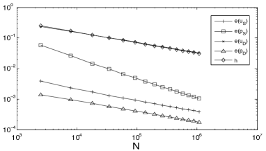
Figure 1: MINI–BDM(1) coupling (left) and Bernardi-Raugel–RT(0) coupling (right).

Table 3: Convergence rates.

		MINI–BDM(1)				MINI–RT(0)
$h_{\textrm{S}}$	$h_{\textrm{D}}$	$r(\textbf{u}_{\textrm{S}})$	$r(\textbf{u}_{\textrm{D}})$	$r(p_{\textrm{S}})$	$r(p_{\textrm{D}})$	$r(\textbf{u}_{\textrm{S}})$	$r(\textbf{u}_{\textrm{D}})$	$r(p_{\textrm{S}})$	$r(p_{\textrm{D}})$
$1/6$	$1/12$	$-$	$-$	$-$	$-$	$-$	$-$	$-$	$-$
$1/10$	$1/20$	1.091	0.983	1.990	1.017	1.091	0.979	1.990	0.988
$1/14$	$1/28$	1.063	0.993	1.955	1.010	1.063	0.991	1.955	0.995
$1/18$	$1/36$	1.047	0.996	1.926	1.006	1.047	0.995	1.926	0.997

Table 4: Convergence rates.

		MINI–BDM(1)				MINI–RT(0)
$h_{\textrm{S}}$	$h_{\textrm{D}}$	$r(\textbf{u}_{\textrm{S}})$	$r(\textbf{u}_{\textrm{D}})$	$r(p_{\textrm{S}})$	$r(p_{\textrm{D}})$	$r(\textbf{u}_{\textrm{S}})$	$r(\textbf{u}_{\textrm{D}})$	$r(p_{\textrm{S}})$	$r(p_{\textrm{D}})$
$1/12$	$1/6$	$-$	$-$	$-$	$-$	$-$	$-$	$-$	$-$
$1/20$	$1/10$	1.063	0.933	1.907	0.996	1.061	0.921	1.907	0.951
$1/28$	$1/14$	1.037	0.971	1.856	1.021	1.037	0.966	1.856	0.980
$1/36$	$1/18$	1.027	0.984	1.824	1.018	1.026	0.981	1.824	0.989

We now describe the data of the example. We consider the domains $\Omega_{\mathrm{D}}:=(0,1)^{2}\times(0,0.5)^{3}$ and $\Omega_{\mathrm{S}}:=(0,1)^{2}\times(0.5,1)$, and take $\nu=1$, $\kappa=1$ and $\textbf{K}=\textbf{I}$, the identity of $\mathbb{R}^{3\times 3}$. Non-homogeneous transmission conditions are considered in order to have an exact solution given by:

$$p_{\textrm{D}}(\boldsymbol{x}):=x_{1}(1-x_{1})\sin(2\pi x_{1})\,x_{2}(1-x_{2})\sin(2\pi x_{2})\,x_{3}\sin(2\pi x_{3})-p_{\textrm{D}0}\,,$$

in the porous media and by

$$\textbf{u}_{\textrm{S}}(\boldsymbol{x}):=x_{1}(1-x_{1})x_{2}(1-x_{2})x_{3}(1-x_{3})\left(\begin{array}[]{c}-2x_{1}(1-x_{1})(1-2x_{2})(1-2x_{3})\\ x_{2}(1-x_{2})(1-2x_{1})(1-2x_{3})\\ x_{3}(1-x_{3})(1-2x_{1})(1-2x_{2})\end{array}\right)\,,$$

and

$$p_{\textrm{S}}(\boldsymbol{x}):=\exp(x_{1}+x_{2}+x_{3})\>,$$

in the Stokes domain.

Table 5: Convergence rates.

		Bernardi-Raugel–BDM(1)				Bernardi-Raugel–RT(0)
$h_{\textrm{S}}$	$h_{\textrm{D}}$	$r(\textbf{u}_{\textrm{S}})$	$r(\textbf{u}_{\textrm{D}})$	$r(p_{\textrm{S}})$	$r(p_{\textrm{D}})$	$r(\textbf{u}_{\textrm{S}})$	$r(\textbf{u}_{\textrm{D}})$	$r(p_{\textrm{S}})$	$r(p_{\textrm{D}})$
$1/6$	$1/12$	$-$	$-$	$-$	$-$	$-$	$-$	$-$	$-$
$1/10$	$1/20$	1.537	0.983	1.034	1.020	1.537	0.979	1.038	0.991
$1/14$	$1/28$	1.574	0.993	1.021	1.011	1.574	0.991	1.021	0.996
$1/18$	$1/36$	1.574	0.996	1.014	1.007	1.574	0.995	1.014	0.998

Table 6: Convergence rates.

		Bernardi-Raugel–BDM(1)				Bernardi-Raugel–RT(0)
$h_{\textrm{S}}$	$h_{\textrm{D}}$	$r(\textbf{u}_{\textrm{S}})$	$r(\textbf{u}_{\textrm{D}})$	$r(p_{\textrm{S}})$	$r(p_{\textrm{D}})$	$r(\textbf{u}_{\textrm{S}})$	$r(\textbf{u}_{\textrm{D}})$	$r(p_{\textrm{S}})$	$r(p_{\textrm{D}})$
$1/12$	$1/6$	$-$	$-$	$-$	$-$	$-$	$-$	$-$	$-$
$1/20$	$1/10$	1.573	0.933	1.014	0.996	1.573	0.921	1.014	0.951
$1/28$	$1/14$	1.543	0.971	1.008	1.021	1.543	0.966	1.008	0.980
$1/36$	$1/18$	1.503	0.984	1.005	1.018	1.503	0.981	1.005	0.989

The numerical results were obtained using a MATLAB code. In Figure 1 we summarize the convergence history of the Galerkin scheme (3.4) for a sequence of uniform meshes of the computational domain $\Omega:=(0,1)^{3}$ by means of tetrahedra. We select the conforming example consisting in the MINI–BDM(1) coupling and the nonconforming example given by the Bernardi-Raugel–RT(0) coupling. In each case we display the individual errors versus the degrees of freedom $N$. We observe that, as expected, the convergence is linear with respect to the discretization parameter $h$ in all the unknowns unless for the fluid pressure in the MINI–BDM(1) example where a quadratic convergence is attained. We notice that the Bernardi-Raugel–RT(0) case delivers a convergence in the fluid velocity that is slightly faster than $O(h)$.

We also provide numerical results for triangulations with hanging nodes on the transmission interface. We consider, uniform triangulations of the subdomains $\Omega_{D}:=(0,1/2)^{3}$ and $\Omega_{S}:=(1/2,1)^{3}$ with a mesh size in one of the subdomains equal to half the mesh size in the other one. The expected rates of convergence are attained in all the (conforming and non-conforming) cases considered through Tables 3, 4, 5 and 6.

Summarizing, the numerical results presented here constitute enough support to our theory for the strong mixed finite element coupling of Darcy–Stokes flow problem. In a forthcoming work we will discuss an efficient iterative method to solve the linear system of equations arising from our discretization method.

References

- [1] R. A. Adams and J. J. F. Fournier. Sobolev spaces, volume 140 of Pure and Applied Mathematics (Amsterdam). Elsevier/Academic Press, Amsterdam, second edition, 2003.
- [2] G. Beavers and D. Joseph. Boundary conditions at a naturally impermeable wall. Journal of Fluid Mechanics, 30:197–207, 1967.
- [3] C. Bernardi, T. Chacón Rebollo, F. Hecht, and Z. Mghazli. Mortar finite element discretization of a model coupling Darcy and Stokes equations. M2AN Math. Model. Numer. Anal., 42(3):375–410, 2008.
- [4] S. C. Brenner and L. R. Scott. The mathematical theory of finite element methods, volume 15 of Texts in Applied Mathematics. Springer, New York, third edition, 2008.
- [5] F. Brezzi and M. Fortin. Mixed and hybrid finite element methods, volume 15 of Springer Series in Computational Mathematics. Springer-Verlag, New York, 1991.
- [6] E. Burman and P. Hansbo. A unified stabilized method for Stokes’ and Darcy’s equations. J. Comput. Appl. Math., 198(1):35–51, 2007.
- [7] M. Discacciati, E. Miglio, and A. Quarteroni. Mathematical and numerical models for coupling surface and groundwater flows. Appl. Numer. Math., 43(1-2):57–74, 2002.
- [8] V. Domínguez and F.-J. Sayas. Stability of discrete liftings. C. R. Math. Acad. Sci. Paris, 337(12):805–808, 2003.
- [9] A. Ern and J.-L. Guermond. Theory and practice of finite elements, volume 159 of Applied Mathematical Sciences. Springer-Verlag, New York, 2004.
- [10] G. N. Gatica, S. Meddahi, and R. Oyarzúa. A conforming mixed finite-element method for the coupling of fluid flow with porous media flow. IMA J. Numer. Anal., 29(1):86–108, 2009.
- [11] G. N. Gatica, R. Oyarzúa, and F.-J. Sayas. Analysis of fully-mixed finite element methods for the Stokes-Darcy coupled problem. Math. Comp., 80(276):1911–1948, 2011.
- [12] G. N. Gatica, R. Oyarzúa, and F.-J. Sayas. Convergence of a family of Galerkin discretizations for the Stokes-Darcy coupled problem. Numer. Methods Partial Differential Equations, 27(3):721–748, 2011.
- [13] G. N. Gatica and F.-J. Sayas. Characterizing the inf-sup condition on product spaces. Numer. Math., 109(2):209–231, 2008.
- [14] V. Girault and P.-A. Raviart. Finite element methods for Navier-Stokes equations, volume 5 of Springer Series in Computational Mathematics. Springer-Verlag, Berlin, 1986. Theory and algorithms.
- [15] P. Grisvard. Singularities in boundary value problems, volume 22 of Recherches en Mathématiques Appliquées [Research in Applied Mathematics]. Masson, Paris, 1992.
- [16] W. Jäger and M. Mikelic. On the interface boundary condition of Beavers, Joseph and Saffman. SIAM Journal on Applied Mathematics, 60:1111–1127, 2000.
- [17] T. Karper, K.-A. Mardal, and R. Winther. Unified finite element discretizations of coupled Darcy-Stokes flow. Numer. Methods Partial Differential Equations, 25(2):311–326, 2009.
- [18] W. Layton, F. Schieweck, and I. Yotov. Coupling fluid flow with porous media flow. SIAM Journal on Numerical Analysis, 40(6):2195–2218, 2003.
- [19] B. Rivière. Analysis of a discontinuous finite element method for coupled Stokes and Darcy problems. Appl. Numer. Math., 22-23:479–500, 2005.
- [20] P. Saffman. On the boundary condition at a surface of porous media. Studies in Applied Mathematics, 50:93–101, 1971.
- [21] L. R. Scott and S. Zhang. Finite element interpolation of nonsmooth functions satisfying boundary conditions. Math. Comp., 54(190):483–493, 1990.