Particle motion in a deformed potential using a transformed oscillator basis

Abstract

The quantum description of a particle moving in a deformed potential is investigated. A pseudostate (PS) basis is used to represent the states of the composite system. This PS basis is obtained by diagonalizing the system Hamiltonian in a family of square integrable functions. In this work the Transformed Harmonic Oscillator (THO) functions, obtained from the solutions of the Harmonic Oscillator using a Local Scale Transformation (LST), are used. The proposed method is applied to the ¹¹Be nucleus, treated in a two-body model (${}^{10}{\rm Be}+n$). Both structure and reaction observables have been studied.

Wavefunctions and energies obtained for the bound states and some low-lying resonances are compared with those obtained by direct integration of the Schrödinger equation. The dipole and quadrupole electric transition probabilities for the low-energy continuum have been calculated in the THO basis, and compared with the exact distributions obtained with the scattering states. Finally, the method is applied to describe the ¹¹Be states in the Coulomb breakup of ¹¹Be+²⁰⁸Pb at 69 MeV/nucleon. The energy and angular distributions of the exclusive breakup have been calculated using the Equivalent Photon Method, including both E1 and E2 contributions. The calculated distributions are found to be in good agreement with the available experimental data from RIKEN [Phys. Rev. C70, 054606]. At the very forward angles, the cross section is completely dominated by the dipole couplings.

I Introduction

It is well known that the quantum collision of a weakly bound system by a target is influenced by the coupling to the unbound states of the projectile. For nuclear collisions, this effect was first noticed in deuteron-induced reactions, and later observed in the scattering of other loosely bound nuclei, such as halo nuclei. Several reaction frameworks have been envisaged to account for this effect. Among them, one of the most successful has been the Continuum-Discretized Coupled-Channels (CDCC) method Rawitscher (1974); Austern et al. (1987), originally developed to account for the breakup channels in deuteron scattering and later extended to other weakly-bound nuclei, such as ^6,7Li, ¹¹Be, or ⁸B, among others. In all these cases, the projectile is described in a two-body model (⁶Li=⁴He+$d$, ⁷Li=⁴He+³H, ¹¹Be=¹⁰Be+$n$, etc) and the method considers explicitly the possible dissociation of the projectile into its two fragments. In its standard formulation, the excitation of each fragment is nevertheless ignored. This is a good approximation for deuteron scattering, for which both constituents can be considered inert at the energies of interest in nuclear studies, but it is more questionable for more complex systems. Moreover, the bound and unbound states of the two-body system are considered to be well described by pure single-particle configurations. This approximation ignores possible admixtures of different core states in the wave functions of the projectile. These admixtures are known to be important, particularly in the case of well-deformed cores, as for example in the ¹¹Be halo nucleus.

A recent attempt to accommodate these effects within the CDCC method was done in Ref. Summers et al. (2006), and applied to the scattering of one-neutron halo nuclei. In that work, the states of the core+valence system were described within the particle-rotor model Bohr and Mottelson (1969). The unbound states of the compound system were described by continuum bins which, following the standard procedure, were constructed by superposition of scattering states. These scattering states are obtained by direct integration of the Schrödinger equation, with the appropriate boundary conditions.

Alternatively, the bound and unbound states of the system can be obtained by diagonalizing the Hamiltonian in a suitable basis of square-integrable functions. The eigenfunctions of the system are expressed as an expansion in the basis functions. In practical calculations, the basis needs to be truncated, leading to a finite expansion of the eigenfunctions. Therefore, these states and their corresponding eigenvalues can be regarded as a finite approximation to the exact states of the system and are referred hereafter as pseudo-states (PS). This procedure has been applied, for example, to describe the states of two-body nuclei interacting via a central potential Matsumoto et al. (2003); Pérez-Bernal et al. (2002); Moro et al. (2009) and, more recently, also for three-body nuclei Matsumoto et al. (2004a, b); Matsumoto et al. (2006); Rodríguez-Gallardo et al. (2008). A variety of bases have been used in these applications, such as harmonic oscillator (HO), Gaussian, Laguerre functions, etc. The procedure can be also extended to deformed systems. A natural choice for the PS would be the deformed HO potential Vautherin (1973); Gambhir et al. (1990). However, this basis is not suitable to describe the bound states of weakly-bound nuclei due to its Gaussian asymptotic behavior. Several alternatives have been proposed in the literature, for example, the eigenstates of a truncated Woods-Saxon potential Zhou et al. (2003) or the Sturmian basis Bang and Vaagen (1980); Nunes et al. (1996).

In this work, we propose the use of a Transformed Harmonic Oscillator (THO) basis to describe the states of a two-body system mutually interacting with a deformed potential. This basis has been previously applied to the case of spherical systems Moro et al. (2009) so we present here its extension to deformed systems. The THO basis is obtained by applying a Local Scale Transformation (LST) to the Harmonic Oscillator (HO) basis. The LST, adopted from a previous work of Karataglidis et al. Karataglidis et al. (2005), is such that it transforms the Gaussian asymptotic behavior into an exponential form, thus ensuring the correct asymptotic behavior for the bound wave functions. The accuracy of this THO basis was tested for several reactions induced by deuteron and halo nuclei, showing an excellent agreement with the standard binning method, and an improved convergence rate in the case of narrow resonances Moro et al. (2009); Lay et al. (2010a).

For a deformed potential, the calculation of bound and unbound states becomes a multi-channel problem, since, in general, for each physical state there will be contributions from several orbital angular momenta and core states. For bound states, the calculation of the energies and eigenfunctions is analogous to the single-channel case, because these quantities are directly obtained from the diagonalization in the chosen PS basis. For unbound states, the eigenfunctions (and their corresponding eigenvalues) obtained from the Hamiltonian diagonalization can be regarded as a finite and discrete representation of the exact states. In general, resonances (quasi-stationary states) correspond to combinations of these positive-energy eigenstates and hence its identification is not straightforward.

For a particle moving in a central potential (with possibly a spin-orbit component) this is a relatively straightforward problem and indeed a variety of methods have been proposed to compute resonance energies and widths. For example, they can be obtained from the poles of the $S$-matrix in the complex energy plane. A simpler method is to define the resonance as the energy at which the phase-shift crosses $\pi/2$. The width is then obtained from the inverse of the derivative of the phase-shift, evaluated at the energy of the resonance. These methods rely on the knowledge of the scattering states at large distances (from which the $S$-matrix and hence the phase-shifts can be extracted) and then they cannot be directly applied to PS methods, given the wrong asymptotic behaviour of the PS functions. In this case, the identification of resonances can be done using the so-called stabilization method Hazi and Taylor (1970); Taylor and Hazi (1976). This is a procedure envisaged to identify and construct the most localized continuum wave functions when the positive energy states are expanded in a discrete basis, depending on one or more parameters. In practice, this can be achieved by diagonalizing the Hamiltonian as a function of these parameters (for example, the basis size) and then scanning the resultant eigenvalues for the continual appearance of a stabilized value which, unlike the others, is insensitive to the size of the basis. In some previous works, we have successfully applied this technique to obtain the resonances of two-body systems with central potentials using the THO basis Moro et al. (2009); Lay et al. (2010a). In this work, we explore the validity of this method for the multi-channel situation that arises in the deformed case. Our aim with this work is to assess the capability of the THO basis for calculations including core deformation in the simpler two-body systems, as ¹¹Be. This step is necessary and unavoidable for providing a solid basement to proceed with the generalization of the formalism to more challenging situations, such as the case of three-body composite systems including core deformation, or to the scattering of a two-body system by a third body, including core deformation in one of the clusters of the composite system.

The work is structured as follows. In Section II the THO method based on the parametric LST is reviewed and the structure model used in subsequent calculations is discussed. In Section III, general expressions for the electric transition operators for the particular case of a two-body system with a deformed core are provided. In Sec. IV the model is applied to describe the structure of the ¹¹Be nucleus. The basis so obtained is then used to describe the Coulomb breakup of ¹¹Be on ²⁰⁸Pb at 69 MeV/nucleon, comparing our results with the available data. Finally, in Section V the main results of this work are summarized.

II Eigenstates of a deformed potential in a PS basis: the THO basis

In this section, we briefly review the features of the PS basis used in this work. This basis is an extension of the THO basis used in our previous works to describe the states of a composite system consisting of two interacting inert fragments, such as a valence particle (proton/neutron) and a spherical and stable core. The goal of this extension is to allow core-excited admixtures in the description of the states of the composite system and hence the possibility of dynamic core excitation mechanisms in reactions involving these nuclei. For completeness, we review first the situation in which the core degrees of freedom are neglected. In this case, the core+valence Hamiltonian is simply given by:

$$H=T_{r}+V_{vc}(\vec{r})$$ (1)

where $\vec{r}$ is the relative coordinate between the valence and the core, $T_{r}$ the core-valence kinetic energy operator and $V_{vc}(\vec{r})$ is the interaction between the valence particle and the core. The eigenstates of this Hamiltonian can be characterized by the energy eigenvalues ($\varepsilon$) and the set of quantum numbers $\{\ell,s,j\}$, which correspond to the orbital angular momentum ($\ell$), the valence spin ($s$) and their sum ($\vec{j}=\vec{\ell}+\vec{s}$). For a central potential with, possibly, a spin-orbit term, these states can be written as:

$$\phi_{\varepsilon,\ell,j}(\vec{r})=R_{\varepsilon,\ell,j}(r){\cal Y}_{\ell sjm}(\hat{r})$$ (2)

where ${\cal Y}_{\ell sjm}(\hat{r})=\left[Y_{\ell}(\hat{r})\otimes\chi_{s}\right]_{jm}$, with $\chi_{s}$ a spin function. The radial functions $R_{\varepsilon,\ell j}(r)$ can be obtained by solving the Schrödinger equation subject to the appropriate boundary condition for bound ($\varepsilon<0$) or unbound ($\varepsilon>0$) states. Alternatively, these functions can be obtained by diagonalizing the Hamiltonian (1) in a discrete basis. Since any complete basis will be infinite, this procedure is not feasible in practice unless the basis is truncated. By doing so, one obtains a finite (an approximate) expansion of the functions $R(r)$ in the selected basis. If the basis functions are denoted by $\varphi_{n,\ell,j}(\vec{r})=\chi_{n,\ell}(r){\cal Y}_{\ell sjm}(\hat{r})$, we will have:

$$R_{\beta}(r)=\sum_{n=1}^{N}c_{\beta,n}\chi_{n,\ell}(r)$$ (3)

where $\beta\equiv\{\varepsilon,\ell,s,j\}$ and $N$ is the number of states retained in the basis.

As already mentioned, there are many possible choices for the basis functions $\{\varphi_{n}\}$ (Gaussians, harmonic oscillator, Laguerre, etc). In this work we use the transformed harmonic oscillator (THO) basis, obtained from the harmonic oscillator basis with an appropriate LST Stoitsov and Petkov (1988); Petkov and Stoitsov (1991). If the LST function is denoted by $s(r)$, the THO states are obtained as

$$R^{THO}_{n,\ell}(r)=\sqrt{\frac{ds}{dr}}R^{HO}_{n,\ell}[s(r)],$$ (4)

where $R^{HO}_{n,\ell}(s)$ is the radial part of the HO functions. With the criterion given above, the LST is indeed not unique. In Ref. Pérez-Bernal et al. (2001) the LST was defined in such a way that the first HO state is exactly transformed into the exact ground state wave function, assuming that this is known. Therefore, by construction, this wave function is exactly recovered for any arbitrary size of the basis. In a more recent work Moro et al. (2009) we adopted the parametric form of Karataglidis et al. Karataglidis et al. (2005)

$$s(r)=\frac{1}{\sqrt{2}b}\left[\frac{1}{\left(\frac{1}{r}\right)^{m}+\left(\frac{1}{\gamma\sqrt{r}}\right)^{m}}\right]^{\frac{1}{m}}\ ,$$ (5)

that depends on the parameters $m$, $\gamma$ and the oscillator length $b$. Note that, asymptotically, the function $s(r)$ behaves as $s(r)\sim\frac{\gamma}{b}\sqrt{\frac{r}{2}}$ and hence the functions obtained by applying this LST to the HO basis behave at large distances as $\exp(-\gamma^{2}r/2b^{2})$. Therefore, the ratio $\gamma/b$ can be related to an effective linear momentum, $k_{\mathrm{eff}}=\gamma^{2}/2b^{2}$, which governs the asymptotic behaviour of the THO functions. As the ratio $\gamma/b$ increases, the radial extension of the basis decreases and, consequently, the eigenvalues obtained upon diagonalization of the Hamiltonian in the THO basis tend to concentrate at higher excitation energies. Therefore, $\gamma/b$ determines the density of eigenstates as a function of the excitation energy. In all the calculations presented in this work, the power $m$ has been taken as $m=4$. This choice is discussed in Ref. Karataglidis et al. (2005) where the authors found that the results are weakly dependent on $m$.

Note that, by construction, the family of functions $R^{THO}_{n,\ell}(r)$ are orthogonal and constitute a complete set with the following normalization:

$$\int_{0}^{\infty}r^{2}|R^{THO}_{n,\ell}(r)|^{2}dr=1\,.$$ (6)

Moreover, they decay exponentially at large distances, thus ensuring the correct asymptotic behaviour for the bound wave functions. In practical calculations a finite set of functions (4) is retained, and the internal Hamiltonian of the projectile is diagonalized in this truncated basis with $N$ states, giving rise to a set of eigenvalues and their associated eigenfunctions, denoted respectively by $\left\{\varepsilon_{n}\right\}$ and $\{\varphi^{(N)}_{n,\ell}(r)\}$ ($n=1,\ldots,N$). As the basis size is increased, the eigenstates with negative energy will tend to the exact bound states of the system, while those with positive eigenvalues can be regarded as a finite representation of the unbound states.

The formalism can be extended to the situation in which the core degrees of freedom are taken into account explicitly. In this case, the Hamiltonian (1) is generalized to

$$H=T_{r}+V_{vc}(\vec{r},\vec{\xi})+h_{\rm core}(\vec{\xi})$$ (7)

where $h_{\rm core}(\vec{\xi})$ is the intrinsic Hamiltonian of the core, whose eigenstates will be denoted by $\{\phi_{IM_{I}}\}$. Additional quantum numbers, required to fully specify the core states, are not included for notation simplicity. Note that the valence-target interaction, $V_{vc}(\vec{r},\vec{\xi})$, contains now a dependence on the core degrees of freedom (denoted generically by $\vec{\xi}$).

The eigenstates of the Hamiltonian cannot any longer be written in the form of Eq. (2). Instead, these states will be a superposition of several valence configurations and core states, i.e.

$$\Psi_{\varepsilon;JM}(\vec{r},\vec{\xi})=\sum_{\alpha}R_{\varepsilon,\alpha}(r)\left[{\cal Y}_{\ell sjm}(\hat{r})\otimes\phi_{I}(\vec{\xi})\right]_{JM}.$$ (8)

Upon replacement of the expansion (8) into the Schrödinger equation, one gets a coupled set of differential equations for the radial functions $R_{\varepsilon,\alpha}(r)$. For bound states, these radial functions decay exponentially for $r\rightarrow\infty$ giving rise to square-integrable functions. For continuum states, the functions $R_{\varepsilon,\alpha}(r)$ are also obtained by solving a set of coupled radial equations, but subject to the boundary condition that incident waves occur only in the entrance channel characterized by a given set of quantum numbers $\alpha=\{\ell,s,j,I\}$. Therefore, for each continuum energy, there are as many scattering solutions as possible values of $\alpha$, compatible with the total angular momentum $J$.

Alternatively, the functions $R_{\varepsilon,\alpha}(r)$ can be obtained using an expansion in a PS basis, such as the THO basis described above. In this case, the basis must include also the new core degree of freedom

$$\Phi^{\alpha}_{n,JM}(\vec{r},\vec{\xi})=R^{THO}_{n,\alpha}(r)\left[{\cal Y}_{\ell sjm}(\hat{r})\otimes\phi_{I}(\vec{\xi})\right]_{JM}.$$ (9)

In this basis, the states of the system will be expressed as

$$\Psi^{(N)}_{i,JM}(\vec{r},\vec{\xi})=\sum_{n=1}^{N}\sum_{\alpha}c^{i}_{n,\alpha,J}\Phi^{\alpha}_{n,JM}(\vec{r},\vec{\xi}),$$ (10)

where $i$ is an index that labels the order of the eigenstate.

These eigenstates are spread in the energy spectrum with a density strongly related to the basis parameters, mainly $N$ and $\gamma/b$, and to the continuum structure for the selected Hamiltonian, i.e. presence of resonances or different breakup thresholds. Moreover, this density reflects the momentum distribution of the eigenstates which becomes important to obtain continuous energy or momentum distributions of different observables from their discrete representation in the PS basis Matsumoto et al. (2003); Tostevin et al. (2001); Moro et al. (2009); Lay et al. (2010a). Generalizing the expression in Lay et al. (2010a), the density of states is here defined as:

$$\rho(k)=\sum_{i=1}^{N}\sum_{\alpha}^{n_{\alpha}}\langle k_{\alpha}J_{f}|\Psi^{(N)}_{i,JM}\rangle,$$ (11)

where $|k_{\alpha}J_{f}\rangle$ denotes the exact scattering wavefunction for an incoming wave in the $\alpha$ channel. Note that the difference between $k$ and $k_{\alpha}$ relays on the threshold energy for each channel.

With this definition the integral of the density with respect to the momentum is the number of THO functions selected (N) times the number of channels ($n_{\alpha}$):

$$\int_{0}^{\infty}\rho(k)\,dk=Nn_{\alpha},$$ (12)

assuming that we have included N THO functions for each channel $\alpha$. Note that this integrated density is independent of the LST parameters.

The afore-mentioned method can be applied to any Hamiltonian of the form (7). In the calculations presented in this work, the composite system is treated within the particle-rotor model Bohr and Mottelson (1969). Therefore, we assume that the core nucleus has a permanent deformation which, for simplicity, is taken to be axially symmetric. Thus, we can characterize the deformation by a single parameter $\beta_{2}$. In the body-fixed frame, the surface radius is then parameterized as $R(\hat{\xi})=R_{0}[1+\beta_{2}\,Y_{20}(\hat{\xi})]$, with $R_{0}$ an average radius. Starting from a central potential, $V^{(0)}_{vc}(r)$, the full valence-core interaction is obtained by deforming this interaction as,

$$V_{vc}(\vec{r},\hat{\xi})=V_{vc}^{(0)}(r-\delta_{2}Y_{20}(\hat{\xi})),$$ (13)

with $\delta_{2}=\beta_{2}R_{0}$ being the deformation length. Transforming to the space-fixed frame of reference, and expanding in spherical harmonics, this deformed potential reads

$$V_{vc}(\vec{r},\vec{\xi})=\sum_{{\cal L,M}}V_{vc}^{(\cal L)}(r)Y_{{\cal L}{\cal M}}(\hat{r})Y^{*}_{{\cal L}{\cal M}}(\hat{\xi})~{},$$ (14)

where the radial form factors $V_{vc}^{(\cal L)}(r)$ are obtained by projecting the deformed potential (13) onto the required multipoles.

III Electric transition probabilities in the PS basis

The accuracy of the PS basis to represent the continuum can be studied by comparing the ground-state to continuum transition probability due to a given operator. Here we consider the important case of the electric dissociation of the initial nucleus into the fragments $c+v$. This involves a matrix element between a bound state (typically the ground state) and the continuum states.

The electric transition probability between two bound states $|J_{i}\rangle$ and $|J_{f}\rangle$ (assumed here to be unit normalized) is given by the reduced matrix element (according to Brink and Satchler convention Brink and Satchler (1968))

$${\cal B}(E\lambda;i\to f)=\frac{2J_{f}+1}{2J_{i}+1}\left|\langle J_{f}||\mathcal{M}(E\lambda)||J_{i}\rangle\right|^{2},$$ (15)

where $\mathcal{M}$ is the multipole operator. In a core+valence model, the electric transition operator can be written as a sum of three terms Lay et al. (2010b): one for the excitation of the valence particle outside the core, one for the excitation of the core as a whole and one for mixed excitations involving simultaneous excitations of core and valence particle,

$$\mathcal{M}(E\lambda\mu) = \sum_{k=1}^{\lambda-1}\sum_{m=-k}^{k}f_{\lambda}(k,m,\mu)$$ (16)

$$\times \mathcal{M}_{sp}(Ekm)\mathcal{M}_{core}(E(\lambda-k)(\mu-m))$$

$$+ \mathcal{M}_{sp}(E\lambda\mu)+\mathcal{M}_{core}(E\lambda\mu),$$

where $f_{\lambda}(k,m,\mu)$ is a well-defined function of its indices and the single particle contribution has the usual form,

$$\mathcal{M}_{sp}(E\lambda\mu)=Z_{\mathrm{eff}}^{(\lambda)}er^{\lambda}Y_{\lambda\mu}(\hat{r}),$$ (17)

with the effective charge:

$$Z_{\mathrm{eff}}^{(\lambda)}=Z_{v}\left(\frac{m_{c}}{m_{v}+m_{c}}\right)^{\lambda}+Z_{c}\left(-\frac{m_{v}}{m_{v}+m_{c}}\right)^{\lambda}.$$ (18)

In the case of a transition to a continuum of states, $|kJ_{f}\rangle$, the definition (15) is replaced by (see for example Typel and Baur (2005)):

$$\frac{d{\cal B}(E\lambda)}{d\varepsilon}=\frac{2J_{f}+1}{2J_{i}+1}\frac{\mu_{vc}k}{(2\pi)^{3}\hbar^{2}}\left|\langle kJ_{f}||\mathcal{M}(E\lambda)||J_{i}\rangle\right|^{2},$$ (19)

with $k=\sqrt{2\mu_{bc}\varepsilon}/\hbar$. Note that the extra factor appearing in Eq. (19) with respect to Eq. (15) is consistent with the convention $\langle kJ|k^{\prime}J\rangle=\delta(k-k^{\prime})$ and the asymptotic behaviour,

$$u_{\alpha^{\prime}}({k_{\alpha^{\prime}}},{r}) \xrightarrow{r\rightarrow\infty} \frac{1}{2}ie^{2i\sigma_{l^{\prime}}}\Big{[}\delta_{\alpha^{\prime}\alpha}H_{l}^{*}(k_{\alpha}r)$$ (20)

$$- \left(\frac{v_{\alpha}}{v_{\alpha^{\prime}}}\right)^{\frac{1}{2}}S^{(J)}_{\alpha^{\prime},\alpha}H_{l^{\prime}}(k_{\alpha^{\prime}}r)\Big{]},$$

where $u_{\alpha}(k_{\alpha},r)=R_{\alpha}(k_{\alpha},r)r$ (using an obvious notation where the continuum $\varepsilon$ label has been replaced by a dependence on the corresponding momentum $k$).

Using a finite basis, one may calculate only discrete values for the transition probability. According to Eq. (15), the $B(E\lambda)$ between the ground state (with angular momentum $J_{i}$) and the $n$-th PS is given by

$${\cal B}^{(N)}(E\lambda;\mathrm{g.s.}\to n)=\frac{2J_{f}+1}{2J_{i}+1}\left|\langle\Psi^{(N)}_{n,J_{f}}||\mathcal{M}(E\lambda)||\Psi_{\mathrm{g.s.}}\rangle\right|^{2}.$$ (21)

In order to relate this discrete representation to the continuous distribution (19) one may derive a continuous approximation to (19) by introducing the identity in the truncated PS basis, i.e.

$$I^{(N)}_{JM}=\sum_{n=1}^{N}|\Psi^{(N)}_{n,JM}\rangle\langle\Psi^{(N)}_{n,JM}|.$$ (22)

For $N\to\infty$ this expression tends to the exact identity operator for the Hilbert space spanned by the eigenfunctions of the considered Hamiltonian. By inserting (22) into the exact expression (19) we obtain the approximate continuous distribution,

$$\frac{d{\cal B}(E\lambda)}{d\varepsilon} \simeq \frac{2J_{f}+1}{2J_{i}+1}\frac{\mu_{vc}k}{(2\pi)^{3}\hbar^{2}}$$

$$\times \left|\sum_{n=1}^{N}\langle kJ_{f}|\Psi^{(N)}_{n,J_{f}}\rangle\langle\Psi^{(N)}_{n,J_{f}}||\mathcal{M}(E\lambda)||\Psi_{\mathrm{g.s.}}\rangle\right|^{2}.$$

This approach provides a smoothing procedure to extract continuous distributions, as a function of the asymptotic energy $\varepsilon$ (or, equivalently, the linear momentum $k$), from the discrete distributions obtained with the PS basis Moro et al. (2006, 2009). This is particularly convenient in situations in which the calculation with the scattering states themselves is not possible, such as in the CDCC method.

IV Test example: application to ¹¹Be

IV.1 Energy spectrum and wave functions in the PS basis

As an illustration of the formalism presented in the preceding section, we consider the ¹¹Be nucleus. This choice is motivated by the fact that this nucleus is one of the best known one-neutron halo nuclei. Many of its properties can be understood in a simple two-body model, comprising a valence neutron orbiting a ¹⁰Be core. For example, the ground state ($1/2^{+}$) and the only bound excited state ($1/2^{-}$) are reasonably well described by $2s_{1/2}$ and $1p_{1/2}$ single-particle configurations, relative to the ${}^{10}{\rm Be}({\rm g.s.})$ core. Excited states in the continuum are also reasonably well described in terms of single-particle excitations of the halo neutron outside the ${}^{10}{\rm Be}({\rm g.s.})$ core. This single-particle picture has been extensively used in the literature to explain also reactions induced by this nucleus (see for instance Capel et al. (2004); Howell et al. (2005); Lay et al. (2010a)). However, there are also numerous experimental and theoretical evidences that these low-lying states of ¹¹Be contain significant admixtures of core-excited components Fortier et al. (1999); Winfield et al. (2001); Cappuzzello et al. (2001); Crespo et al. (2011). Consequently, an accurate description of reactions involving this nucleus requires the inclusion of its states beyond the simple single-particle picture.

In the calculations presented in this work, we use the particle-rotor model of Bohr and Mottelson with the ¹¹Be Hamiltonian of Ref. Nunes et al. (1996) (model Be12-b), which consists of a Woods-Saxon central part, with a fixed geometry ($R=2.483$ fm, $a=0.65$ fm) and a parity-dependent strength. The potential contains also a spin-orbit part, whose radial dependence is given by the derivative of the same Woods-Saxon shape, and strength $V_{so}=8.5$ MeV. For the ${}^{10}{\rm Be}$ core, this model assumes a permanent quadrupole deformation $\beta_{2}$=0.67. Only the ground state ($0^{+}$) and the first excited state ($2^{+}$, $E_{x}=3.368$ MeV) are included in the model space. For the valence-core orbital angular momentum, we consider the values $\ell\leq 3$.

To generate the THO basis we use the LST of Eq. (5) with $m=4$, $b=1.6$ fm and $\gamma=1.84$ fm^1/2. The value of $b$ was determined in order to minimize the ground state energy of ¹¹Be in a small THO basis. The factor $\gamma/b$ leads to a $k_{eff}$ compatible with a maximum excitation energy of about 10 MeV, which is enough for the calculations presented below.

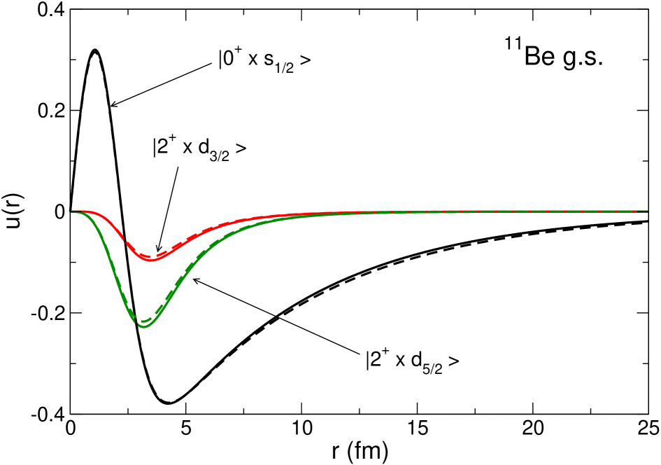
Figure 1: (Colour online) Radial parts of the ground state wave function for the ¹¹Be nucleus obtained by direct integration of the Schrödinger equation (solid lines) and by diagonalization in a THO basis with N=15 states (dashed lines).

Once these parameters have been fixed, the THO basis is generated for different values of N, the number of oscillator functions, and the convergence of different observables is studied with respect to this number. We should remark that the total number of basis functions is this number times the number of channels $n_{\alpha}$. However, the latter depends on the total angular momentum $J$ of the state under consideration, and will be the same in any method based on the angular momentum expansion of the wave functions. Therefore, we will refer to N as the basis size as we understand it is the most honest way of comparing with other methods. We find that the ground-state energy is already fully converged with a relatively small basis (N $\approx 15$).

Within the model space used in our calculations ($I=0,2$, $\ell\leq 3$), there are $n_{\alpha}=3$ channels contributing to the ground state wave function, namely $|^{10}{\rm Be}(0^{+})\otimes s_{1/2}\rangle$, $|^{10}{\rm Be}(2^{+})\otimes d_{3/2}\rangle$ and $|^{10}{\rm Be}(2^{+})\otimes d_{5/2}\rangle$. In Fig. 1, we depict these radial parts of the ground-state wave function obtained from the diagonalization of the Hamiltonian in a THO basis with N=15 oscillator functions (dashed lines). For comparison, we include also the solutions obtained by direct integration of the Schrödinger equation (solid lines). Both calculations give basically identical results. It can be seen, as expected, that the $|^{10}{\rm Be}(0^{+})\otimes s_{1/2}\rangle$ component is the dominant one, accounting for about 80% of the norm. This radial component exhibits a node, due to the presence of a Pauli forbidden state (arising from the $1s_{1/2}$ orbital in the spherical basis).

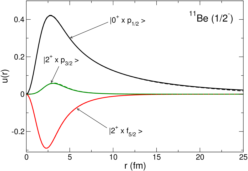
Figure 2: (Colour online) Radial parts of the 1/2^- excited bound state wave function for the ¹¹Be nucleus obtained by direct integration of the Schrödinger equation (solid lines) and by diagonalization in a THO basis with $N=15$ states (dashed lines).

The assumed Hamiltonian reproduces also the position of the bound excited state at $E_{x}=320$ keV ($1/2^{-}$). Indeed, this state appears also in the diagonalization of the THO basis. The separation energy is reproduced within a few percent with a basis of N=15 states and the radial components are also found to be in perfect agreement with those obtained by direct integration of the coupled differential equations. This is shown in Fig. 2.

We proceed to discuss now the description of resonances in the PS basis. As explained in the introduction, the identification of the resonances is done using the stabilization method of Hazi and Taylor Hazi and Taylor (1970); Taylor and Hazi (1976), extended to the multi-channel case. The procedure is the same as in the single-channel case, i.e., we diagonalize the Hamiltonian over either a successively larger basis set or as a function of a continuous parameter which defines the basis for a given N value. Then, the evolution of the spectrum as a function of N or the continuous parameter is studied. When a resonance is present, there are some eigenvalues whose energies are stabilized for a range of values of N or the continuous parameter. This property has been employed empirically in many works, and a formal justification has also been provided by Lippmann and O’Malley Lippmann and O’Malley (1970).

The selected Hamiltonian contains low-lying resonances at $\varepsilon=1.2$ MeV ($5/2^{+}$), 2.7 MeV ($3/2^{-}$) and 3.2 MeV ($3/2^{+}$) Nunes et al. (1996). These values are confirmed applying the stabilization method with the THO basis, in the two ways described above. As an example, in Fig. 3, we show the results for $J^{\pi}=5/2^{+}$. In the upper panel, the sequence of continuum states with $J^{\pi}=5/2^{+}$ is plotted versus the continuum parameter $\gamma$ of the LST, and for a fixed value of N (N=10). In the lower panel, the $J^{\pi}=5/2^{+}$ eigenvalues obtained from the diagonalization of the assumed Hamiltonian in the THO basis are plotted as a function of the discrete basis size parameter (N), with $\gamma$ fixed to 1.84 fm^1/2. The dashed line marks the known location of the first $5/2^{+}$ resonance deduced from the behavior of the phase-shifts and the dotted line marks the $n$+${}^{10}{\rm Be}(2^{+})$ threshold. In both plots, the energy stabilization precisely at the nominal energy of the resonance is apparent. Similar results are obtained for the $3/2^{+}$ and $3/2^{-}$ resonances.

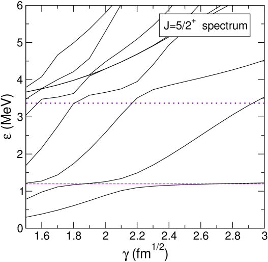
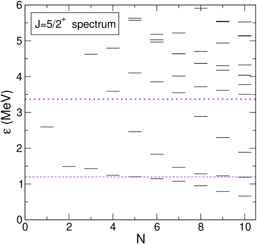
Figure 3: (Colour online) Eigenvalues obtained from the diagonalization of the ¹¹Be Hamiltonian in a THO basis, as a function of the LST continuum parameter ($\gamma$) in the upper panel, and as a function of the number of oscillator states included in the basis in the lower panel. The dashed line indicates the energy of the 5/2⁺ resonance and the dotted line, the energy of the ¹⁰Be(2⁺)+n threshold.

According to the stabilization method, the eigenfunctions corresponding to the stabilized energies should correspond to well localized states, as expected for a resonant state. This is confirmed in Fig. 4 for the three resonances discussed above. In each panel, we compare the radial components of the scattering wave functions evaluated at the nominal energy of the resonance (solid lines), with the THO eigenfunction associated with the stabilized eigenvalue, using a basis of N=10 oscillator functions (dashed lines). Because the continuum wavefunctions are not square-integrable, these functions have been conveniently scaled for a better comparison with the PS functions.

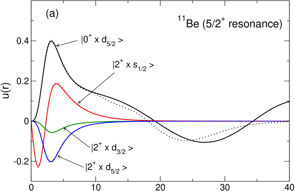
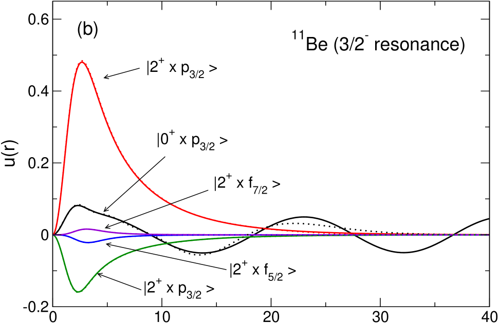
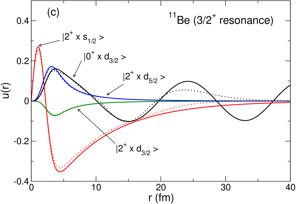
Figure 4: (Colour online) Radial parts of the continuum wave functions for the ¹¹Be resonances at $\varepsilon$=1.2 MeV ($5/2^{+}$), 2.7 MeV ($3/2^{-}$) and 3.2 MeV ($3/2^{+}$). The solid lines are obtained by direct integration of the Schrödinger equation, whereas the dashed lines are the result of the diagonalization in a THO basis with N=10 ($5/2^{+}$) or N=9 ($3/2^{-}$, $3/2^{+}$) oscillator functions. For a better comparison, the normalization of the scattering state has been chosen in order to have the same magnitude as the discrete solution at the maximum.

Note that, for these three resonances, the channels corresponding to $I=2$ are effectively bound, since the energy of these resonances is below the $n$+${}^{10}{\rm Be}(2^{+})$ threshold. The component based on the ${}^{10}{\rm Be}({\rm g.s.})$ is unbound but it shows the anticipated localization reminiscent of a quasi-stationary state. We note that, unlike the case of the bound states, we do not expect a perfect agreement between both calculations due to the exponential behaviour of the PS basis at large distances. Apart from that, it is also seen that, in the interior region, the four radial components are in very good agreement with the exact solution.

The stabilization method provides also expressions for the width of the resonances in the PS basis Taylor and Hazi (1976). However, these expressions were originally developed for the single-channel case, and hence they cannot be directly applied to our case. To have an estimate of the width of the resonance we make use the density of states, defined according to Eq. (11). This function is shown in Fig. 5 for the discussed resonances, using different values of the basis size (N). It can be seen how the density increases as more channels are open above the excitation energy of the core. It can be seen also that the presence of a resonance gives rise to a peak in the density distribution. Based on this property, we have estimated the width of the resonance from the FWHM of the corresponding peak in the density distribution. For the $5/2^{+}$, $3/2^{-}$ and $3/2^{+}$ resonances considered above, this method yields $\Gamma=125$ keV, $40$ keV and $140$ keV respectively. This widths are to be compared with the values reported in Nunes (1995), namely, $\Gamma=125$ keV, $50$ keV and 100 keV. Except for the latter, for which our prescription gives a width 40% larger, the agreement between both methods is very good in the other two cases.

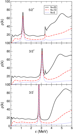
Figure 5: Density of states for the $5/2^{+}$, $3/2^{+}$ and $3/2^{-}$ resonances of the ¹¹Be nucleus, using different values of the basis size N.

Just to complete our study, we show in Fig. 6 the comparison of the radial parts obtained by integration of the Schrödinger equation (solid lines) and by diagonalization in a THO basis with N=15 (dotted lines) for a non-resonant state in the continuum. It can be observed that the agreement is also good for these states.

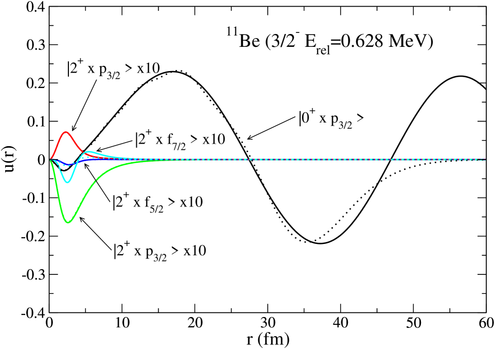
Figure 6: (Colour online) Radial parts of the $3/2^{-}$ wave function for the ¹¹Be nucleus at $E_{rel}=0.628$ MeV obtained by direct integration of the Schrödinger equation (solid lines) and by diagonalization in a THO basis with N=15 states. All the components except the main one are multiplied by a factor of 10.

IV.2 Electric reduced transitions probabilities

The electric transition probabilities provide also a useful test to assess the quality of the basis to represent the continuum states. These transition probabilities can be calculated using either the exact scattering states, using Eq. (19), or the pseudostates, using Eq. (21). In the latter case, one obtains a discrete distribution, which can be converted to a continuous distribution by means of Eq. (III). In actual calculations, this equation is evaluated with a finite number of states (N) and hence this formula is only approximate. The degree of agreement of this approximate formula with the exact calculation provides a measurement of the quality of the PS basis to represent the continuum for a given operator. In this section we perform this test for the E1 and E2 operators.

According to Eq. (16), the electric operator for a valence+core system will contain in general contributions coming from the valence excitation, the core excitation and mixed excitations. However, in our test case, ¹¹Be, with core states restricted to the ground state ($0^{+}$) and the first excited state ($2^{+}$), dipole transitions will consist of pure single particle excitations. On the other hand, quadrupole transitions will contain both single particle and core excitations, but not simultaneous transitions. These simultaneous transitions will only affect octupole and higher order transitions, which will not be considered here.

In Fig. 7, the energy distribution of the ${\cal B}(E1)$ obtained with a THO basis with N=20 functions is shown for ¹¹Be. Separate contributions for $1/2^{-}$ and $3/2^{-}$ states are shown by dotted and dashed lines, respectively. With this basis size, the calculated THO distributions are almost indistinguishable from the exact calculation, obtained with the exact scattering states, so the latter has not been included in the figure. The available experimental distributions from two experiments performed at RIKEN Nakamura et al. (1995) and MSU Palit et al. (2003) are also shown in the plot. The theoretical distribution lies in between the two experimental sets of data. However, one has to keep in mind that the RIKEN data are inclusive with the respect to the ¹⁰Be state and hence it might contain contributions where the core is left in an excited state. Moreover, it is also worth noting that the calculation will be sensitive to the choice of the ¹¹Be Hamiltonian. We have not explored in this work this dependence since the purpose of this calculation is to test the quality of the basis, rather than a detailed comparison with the data.

From Fig. 7 on sees that the calculated distribution shows a dip around $\varepsilon=2.8$ MeV, which is also visible in the data from Ref. Palit et al. (2003). This behavior arises from the presence of the $3/2^{-}$ resonance at this excitation energy. This resonance is relatively narrow ($\Gamma=50$ keV) but it is only weakly coupled because it is mainly built on the excited core (${}^{10}{\rm Be(2^{+})}$), whereas the ground state is mostly ${}^{10}{\rm Be(0^{+})}$.

Because only the single-particle excitation term of Eq. (16) contributes to this dipole transition, this observable can be also well reproduced within a single-particle model of ¹¹Be, with the ¹⁰Be core in its ground state, and including the appropriate spectroscopic factor for the $|^{10}{\rm Be}(0^{+})\otimes 2s_{1/2}\rangle$ configuration. A departure from this behaviour is the afore-mentioned reduction of the ${\cal B}(E1)$ around 2.8 MeV which is due to a core dominated $3/2^{-}$ resonance.

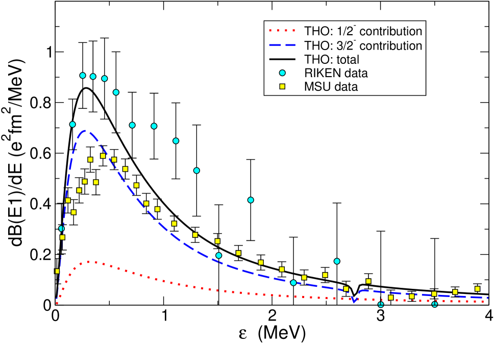
Figure 7: (Colour online) Dipole electric transition probability (${\cal B}(E1)$) obtained with the THO basis and compared with experimental data from RIKEN Nakamura et al. (1995) and MSU Palit et al. (2003). A THO basis with N=20 was used in the calculation, for which the calculated distribution is fully converged and indistinguishable from the exact result using the exact scattering wavefunctions.

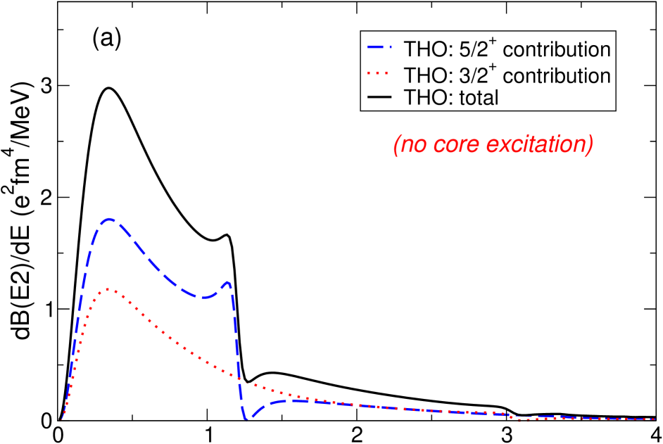
Figure 8: (Colour online) Quadrupole electric transition probability (${\cal B}(E2)$) obtained with the THO basis with N=20 oscillator functions. The upper panel is the calculation including only the valence excitations. The bottom panel includes both valence and core contributions.

We have also evaluated the quadrupole electric transition probabilities, which are shown in Fig. 8. The dotted and dashed lines are the contributions from $3/2^{+}$ and $5/2^{+}$, respectively, whereas the solid line is the sum of both contributions. According to Eq. (16), in addition to the single-particle excitations, in this case we have also a contribution due to E2 transitions of the core which, in fact, give the main contribution to the total ${\cal B}(E2)$ strength. To illustrate better the contribution coming from the valence excitation and the core, we show in the upper panel of this figure the single-particle contribution, whereas in the bottom panel we show the full calculation, including also contributions from the core. It is seen that the ${\cal B}(E2)$ strength is dominated by the core excitations, as expected for a collective transition. The peaks at $\varepsilon\simeq 1.2$ MeV and and $\varepsilon\simeq 3.2$ MeV are due to the $5/2^{+}$ and $3/2^{+}$ resonances. Unfortunately, no experimental or theoretical ${\cal B}(E2)$ for ¹¹Be has been found in the literature in order to compare with.

IV.3 Application to the Coulomb breakup of ¹¹Be on ²⁰⁸Pb

A more recent measurement of the Coulomb breakup of ¹¹Be can be found in the work by Fukuda and collaborators Fukuda et al. (2004), who measured the breakup of a ¹¹Be beam at 69 MeV/nucleon on carbon and lead targets.

At these energies and for very small angles the breakup is dominated by the Coulomb interaction. For angles below the grazing angle the differential break up cross section can be calculated semiclassically using the equivalent photon method (EPM) Bertulani and Baur (1988). For the E1, which is expected to be the dominant one, the breakup cross section in the EPM method reads,

$$\left(\frac{d^{2}\sigma}{d\Omega d\varepsilon}\right)_{bu}=\frac{16\pi^{3}}{9\hbar c}\frac{d{\cal B}(E1)}{d\varepsilon}\frac{dN_{E1}(\theta_{cm},E_{x})}{d\Omega_{cm}},$$ (24)

where $N_{E1}(\theta_{cm},E_{x})$ denotes the number of virtual photons with energy $E_{x}$ at scattering angle $\theta_{cm}$. In this treatment, the scattering angle corresponds to a classical Coulomb trajectory. The photon energy would be always $E_{x}=\varepsilon+S_{1n}$.

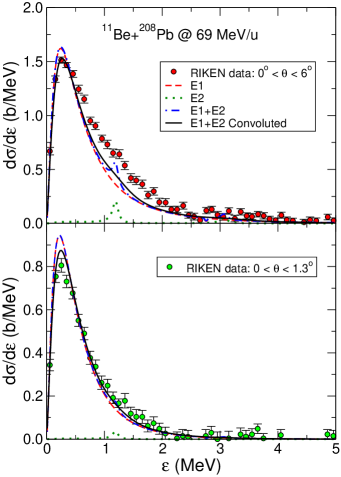
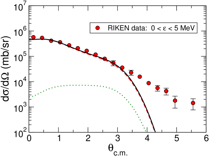
Figure 9: (Colour online) Energy (top panel) and angular (bottom panel) distributions of the exclusive breakup for the reaction ¹¹Be+²⁰⁸Pb at 69 MeV/nucleon. The circles are the experimental data from Ref. Fukuda et al. (2004). The dot-dashed and dashed lines correspond to the E1 and E2 contributions, calculated within the EPM method, and the solid line is the sum of both contributions.

In a similar way, the E2 contribution to the breakup cross section which in this formalism is related to the ${\cal B}(E2)$ distribution,

$$\left(\frac{d^{2}\sigma}{d\Omega d\varepsilon}\right)_{bu}=\frac{4\pi^{3}}{75\hbar c}\left(\frac{E_{x}}{\hbar c}\right)^{3}\frac{d{\cal B}(E2)}{d\varepsilon}\frac{dN_{E2}}{d\Omega_{cm}}.$$ (25)

This contribution should be added to the dipole Coulomb break up. The equivalent photon number for $E2$ transitions can also be found in Bertulani and Baur (1988).

We have evaluated these contributions using the ${\cal B}(E1)$ and ${\cal B}(E2)$ distributions obtained with the THO basis. Indeed, these expressions could be directly evaluated with the scattering states, since no discretization is required in this case. It is nevertheless illustrative to compare both calculations, to show the convergence of these observables with the size of the THO basis. In more sophisticated reaction models, such as the CDCC method with core excitation Summers et al. (2006), the use of a discretization method is mandatory, and hence the use of a discrete basis, like the THO proposed here, is more justified.

From the expressions (24) and (25), the energy and angular differential breakup cross sections are calculated by integrating in the scattering angle or in the excitation energy, respectively. In the former case, a critical ingredient of the calculation is the minimum impact parameter ($b_{\mathrm{min}}$). The model assumes that pure Coulomb breakup occurs only for $b>b_{\mathrm{min}}$. By contrast, for $b<b_{\mathrm{min}}$, the model assumes that other reaction mechanisms rather than pure Coulomb scattering take place (such as nuclear effects). Since these effects are not properly described by Eqs. (24) and (25), these expressions are only evaluated for $b>b_{\mathrm{min}}$. This is also the reason why these Coulomb breakup experiments are focused at small angles, ideally below the grazing angle. In all the calculations the minimum impact parameter is settled according to the choice done in Fukuda et al. (2004), where the (E1) Coulomb breakup cross section is also evaluated using the EPM method.

In Fig. 9 we compare the calculated energy (upper two-panel figure) and angular differential cross sections (lower panel) with the experimental data. The separate E1 and E2 contributions, as well as their sum, are shown in each panel. The calculations have been convoluted with the experimental angular and energy distributions reported in Fukuda et al. (2004). It is clearly seen that the main contribution comes from the dipole break up. In the angular distribution, the sum of both contributions cannot be distinguished at the smaller angles from the pure E1 contribution. The small E2 contribution is only observed in the energy regions of the resonances. This difference is nevertheless washed out once the energy resolution of the experiment is considered. Despite this small contribution, it is observed that the E2 component improves the agreement in the energy region nearby the $5/2^{+}$ resonance. Comparing the total and dipole angular distributions of the Coulomb break up one can infer up to what angle one should consider pure E1 excitations in order to extract a ${\cal B}(E1)$ distribution not affected by the 5/2⁺ resonance.

V Summary and conclusions

We have investigated the problem of the description of the states of a particle moving in a deformed potential in terms of a pseudo-state (PS) basis. In the PS method, the states of the system are approximated by the eigenstates of the Hamiltonian in a basis of square-integrable functions. The negative eigenvalues are identified with the bound states of the system, whereas the positive eigenvalues are regarded as a discrete and finite representation of the continuum spectrum. Identification of resonances is done using the so-called stabilization method Hazi and Taylor (1970); Taylor and Hazi (1976).

Following our previous choice for non-deformed systems, we propose to use as PS basis the Transformed Harmonic Oscillator (THO) basis. The basis functions are obtained by applying an analytic local scale transformation Karataglidis et al. (2005); Moro et al. (2009) to the conventional HO basis. The transformation is such that it converts the Gaussian asymptotic behavior of the HO function into an exponential.

The method has been applied to the ¹¹Be nucleus, treated within a particle-rotor model. The ¹⁰Be core is assumed to have a permanent axial deformation with $\beta_{2}=0.67$ Nunes et al. (1996). We have shown that the bound-state energies and wave functions are very well described using a relatively small basis, showing perfect agreement with those obtained by direct integration of the Schrödinger equation. We have shown that the resonances $5/2^{+}$, $3/2^{-}$ and $3/2^{+}$ are also well described with the method using small THO bases. It has also been checked that the wave functions of the non-resonant continuum calculated with the THO method compare well with the state computed by direct integration of the Schrödinger equation at the same energy.

We have given expressions for the E1 and E2 electric transition probabilities in the discrete basis, and we have proposed a method to obtain smooth distributions from these discrete values. To illustrate this method, we have calculated the ${\cal B}(E1)$ and ${\cal B}(E2)$ electric transition probabilities for the ¹¹Be nucleus. These distributions show a fast convergence rate with the basis size, and the converged results are in perfect agreement with the exact calculation, obtained with the exact scattering states. With the adopted Hamiltonian, the calculated ${\cal B}(E1)$ distribution is consistent, but somewhat larger, than the experimental data from MSU Palit et al. (2003).

Finally, we have applied the model to the Coulomb breakup of ¹¹Be on ²⁰⁸Pb at 69 MeV/nucleon, comparing with the data from Ref. Fukuda et al. (2004). The reaction is treated in a semi-classical picture, using the equivalent photon method, and including both E1 and E2 contributions. The calculated angular distribution is in good agreement with the data for scattering angles below $3^{\circ}$. Beyond this angle, other effects not considered in the EPM method, such as nuclear breakup, are expected to take place. The calculated energy distribution is also in good agreement with the data, particularly when the angular range is below the grazing angle.

We conclude that the THO basis provides a suitable representation to describe two-body composite systems (bound and unbound states) including the core deformation. This study provides the needed test for accomplishing a similar study for more interesting cases, such as three-body composite systems including core deformation or three-body scattering problems (two-body projectile plus a target) including dynamic core excitation. Work toward this direction is in progress.