A decomposition theorem for Herman maps

Abstract.

In 1980s, Thurston established a topological characterization theorem for postcritically finite rational maps. In this paper, a decomposition theorem for a class of postcritically infinite branched covering termed ‘Herman map’ is developed. It’s shown that every Herman map can be decomposed along a stable multicurve into finitely many Siegel maps and Thurston maps, such that the combinations and rational realizations of these resulting maps essentially dominate the original one. This result gives an answer to a problem of McMullen in a sense and enables us to prove a Thurston-type theorem for rational maps with Herman rings.

1. Introduction

In 1980s, Douady and Hubbard [DH1] revealed the complexity of the family of quadratic polynomials. Contemporaneously, Thurston’s 3-dimensional insights revolutionized the theory of Kleinian group [Th1]. After then, Sullivan [Su] discovered a dictionary between these two objects. Applying quasiconformal method to rational maps, he translated the Ahlfors’ finiteness theorem into a solution of a long-outstanding problem of wandering domains.

Based on Sullivan’s dictionary, McMullen asked a question: Is there a 3-dimensional geometric object naturally associated to a rational map? For example, it’s known that Haken manifolds have a hierarchy, where they can be split up into 3-balls along incompressible surfaces. McMullen suggested to translate the Haken theory on cutting along general incompressible subsurfaces into a theory for rational maps with disconnected Julia sets. He posed the following problem ([Mc1], Problem 5.4):

Problem 1.1 (McMullen).

Develop decomposition and combination theorems for rational maps.

In this article, we aim to answer this problem in a sense. We will develop a decomposition theorem for rational maps with Herman rings, or more generally for ‘Herman maps’. Roughly speaking, a Herman map is a postcritically infinite branched covering with ‘Herman rings’ and postcritically finite outside the closure of all rotation domains. We will show that a Herman map can always be decomposed along a stable multicurve into two kinds of ‘simpler’ maps –Siegel maps and Thurston maps, such that the combinations and rational realizations of these ‘simpler’ maps essentially dominate the original one. Here, roughly, a Siegel map is a postcritically infinite branched covering with ‘Siegel disks’ and postcritically finite outside the closure of all ‘Siegel disks’, a Thurston map is a postcritically finite branched covering. The precise formulation of the decomposition theorem requires a fair number of definitions and is put in the next section.

The significance of the decomposition theorem is that it gives a way to extend Thurston’s theory beyond postcritically finite setting. The theory deals with the following problem: Given a branched covering, when it is equivalent (in a proper sense) to a rational map? Thurston [Th2] gave a complete answer to this problem for postcritically finite cases in 1980s by showing that such a map either is equivalent to an essentially unique rational map or contains a ‘Thurston obstruction’. Here, an obstruction is a collection of Jordan curves such that a certain associated matrix has leading eigenvalue greater than 1. The detailed proof of Thurston’s theorem is given by Douady and Hubbard [DH2] in 1993. The insights produce many new, sometimes unexpected applications in complex dynamics [BFH, Br, C, CT1, E, Ge, Go, HSS, P1, R1, R2, R3, Se, ST, T1, T2]… Since then, many people have tried to extend Thurston’s theorem beyond postcritically finite rational maps. Recently, progress has made for several families of holomorphic maps. For example, Hubbard, Schleicher and Shishikura [HSS] extended Thurston’s theorem to postsingularly finite exponential maps $\lambda e^{z}$; Cui and Tan [CT1], Zhang and Jiang [ZJ], independently, proved a Thurston-type theorem for hyperbolic rational maps; other extensions include geometrically finite rational maps and rational maps with Siegel disks [CT2, Z2],…

The decomposition theorem enables us to extend Thurston’s theorem to rational maps with Herman rings. More generally, we have:

Thurston-type theorems for rational maps with Herman rings can be reduced to Thurston-type theorems for rational maps with Siegel disks.

Besides, the decomposition theorem reveals an analogue between Haken manifolds and Herman maps (compare [Mc1, P1]):

Haken manifold	Herman map
incompressible surfaces (I.S.)	stable multicurve
cutting along I.S.	decomposition along stable multicurve
finite procedure to find an I.S.	finite iterate to get a stable multicurve
resulting pieces are 3-balls	resulting maps are Siegel/Thurston maps
reducing theorems to 3-balls	reducing theorems to Siegel/Thurston maps
combination theorem	build up rational map from renormalizations
rigidity theorem	rigidity theorem
hyperbolic structure	rational realization

2. Definitions and main theorems

Let $S^{2}$ be the two-sphere and $f:S^{2}\rightarrow S^{2}$ be an orientation preserving branched covering of degree at leat two. We denote by $\deg(f,x)$ the local degree of $f$ at $x\in S^{2}$. The critical set $\Omega_{f}$ of $f$ is defined by

$$\Omega_{f}=\{x\in S^{2};\deg(f,x)>1\},$$

and the postcritical set $P_{f}$ of $f$ is defined by

$$P_{f}=\overline{\bigcup_{n\geq 1}f^{n}(\Omega_{f})}.$$

We say that $f$ is postcritically finite if $P_{f}$ is a finite set. Such a map is also called a Thurston map. For a Thurston map, we define a function $\nu_{f}:S^{2}\rightarrow\mathbb{N}\cup\{\infty\}$ in the following way: For each $x\in S^{2}$, define $\nu_{f}(x)$ (may be $\infty$) as the least common multiple of the local degrees $\deg(f^{n},y)$ for all $n>0$ and all $y\in S^{2}$ such that $f^{n}(y)=x$. Note that $\nu_{f}(x)=1$ if $x\notin P_{f}$. We call $\mathcal{O}_{f}=(S^{2},\nu_{f})$ the orbifold of $f$.

In the following, we will define two classes of postcritically infinite branched covering–Herman map and Siegel map–step by step. These maps are branched coverings with ‘rotation domains’ and postcritically finite elsewhere. Since the branched covering $f$ will be required to have certain regularity (e.g. ‘holomorphic’ or ‘quasi-regular’) in some parts of the two-sphere $S^{2}$, it is reasonable to equip $S^{2}$ with a complex structure. For this, we will identify $S^{2}$ with $\mathbb{\overline{C}}=\mathbb{C}\cup\{\infty\}$ in our discussion.

Definition 2.1 (Rotation domain).

We say $\langle U_{0},\cdots,U_{p-1}\rangle$ is a cycle of rotation disks (resp. annuli) of $f$ if

1. All $U_{i}$ are disks (resp. annuli), with disjoint closures. Each boundary component of $U_{i}$ is a Jordan curve.

2. $f$ should induce conformal isomorphisms $U_{0}\xrightarrow[]{\cong}U_{1}\xrightarrow[]{\cong}\cdots\xrightarrow[]{\cong}U_{p-1}\xrightarrow[]{\cong}U_{p}=U_{0}$ and the return map $f^{p}:U_{0}\rightarrow U_{0}$ is conformally conjugate to an irrational rotation $z\mapsto e^{2\pi i\theta}z$.

3. Each boundary cycle of $U_{i}$ contains at least one critical point of $f$.

By definition, two different cycles of rotation domains have disjoint closures. Moreover, in the case that all $U_{i}$ are annuli, the union $\cup_{0\leq j<p}\partial U_{j}$ consists of two cycles of boundary curves, thus there are at least two critical points on $\cup_{0\leq j<p}\partial U_{j}$.

One may compare this definition with the definitions of Siegel disks and Herman rings for rational maps in [M]. In general, for rational maps, whether the boundary of a rotation domain contains a critical point depends on the rotation number. It’s known from Graczyk and Swiatek [GS] that for any rational map, the boundary of a Siegel disk (or Herman ring) with bounded type rotation number always contains a critical point. On the other hand, there exist quadratic polynomials with Siegel disks whose boundaries do not contain any critical point (see [H2] or [ABC]). We remark that in Definition 2.1, whether the boundary of a rotation domain contains a critical point is not essential, we need such an assumption simply because we want to concentrate on the combination of the branched covering rather than the complexity caused by the rotation number. Our method can be easily generalized.

Definition 2.2 (Herman map and Siegel map).

We say that $f$ is a Herman map if $f$ has at least one cycle of rotation annuli and postcritically finite outside the union of all rotation domains; a Siegel map if $f$ has at least one cycle of rotation disks and postcritically finite outside the union of all rotation disks.

Note that a Herman map may have rotation disks and a Siegel map has no rotation annuli.

The category of branched covering consisting of Herman maps, Siegel maps and Thurston maps are called HST maps. Namely, a HST map is an orientation preserving branched cover such that each critical orbit either is finite or meets the closure of some rotation domain (if any). Given a HST map $f$, let $n_{RD}(f)$ be the number of rotation disk cycles, $n_{RA}(f)$ be the number of rotation annulus cycles, they satisfy $n_{RD}(f)+2n_{RA}(f)\leq 2\mathrm{deg}(f)-2.$ Obviously, a Thurston map $f$ is a HST map with $n_{RD}(f)=n_{RA}(f)=0$. The union of all rotation domains of $f$ is denoted by $R_{f}$ (probably empty).

Definition 2.3 (Marked set).

Let $f$ be a HST map. A marked set $P$ is a compact set that satisfies the following:

1. $f(P)\subset P$.

2. $P\supset P_{f}\cup\overline{R_{f}}$ and $P-(P_{f}\cup\overline{R_{f}})$ is a finite set.

In this paper, we always use a pair $(f,P)$, a branched covering together with a marked set, to denote a HST map.

Definition 2.4 (C-equivalence and q.c-equivalence).

Two HST maps $(f,P)$ and $(g,Q)$ are called combinatorially equivalent or ‘c-equivalent’ for short (resp. q.c-equivalent), if there is a pair $(\phi,\psi)$ of homeomorphisms (resp. quasi-conformal maps) of $\mathbb{\overline{C}}$ such that

1. $\phi\circ f=g\circ\psi$ and $\phi(P)=Q$.

2. $\phi$ and $\psi$ are holomorphic in $R_{f}$.

3. $\phi$ and $\psi$ are isotopic rel $P$. That is, there is a continuous map $H:[0,1]\times\mathbb{\overline{C}}\rightarrow\mathbb{\overline{C}}$ such that for any $t\in[0,1]$, $H(t,\cdot):\mathbb{\overline{C}}\rightarrow\mathbb{\overline{C}}$ is a homeomorphism, $H(0,\cdot)=\phi,H(1,\cdot)=\psi$ and $H(t,z)=\phi(z)$ for any $t\in[0,1]$ and any $z\in P$.

In this case, we say that $(f,P)$ is c-equivalent (resp. q.c-equivalent) to $(g,Q)$ via $(\phi,\psi)$. If $(g,Q)$ is a rational map, we call $(g,Q)$ a rational realization (resp. q.c-rational realization) of $(f,P)$. Note that if $(f,P)$ has a q.c-rational realization, then $(f,P)$ is necessarily a quasi-regular map.

A Jordan curve $\gamma\subset\mathbb{\overline{C}}\setminus P$ is called null-homotopic, (resp. peripheral) if a component of $\mathbb{\overline{C}}\setminus\gamma$ contains no (resp. one) point of $P$; non-peripheral (or essential) if each component of $\mathbb{\overline{C}}\setminus\gamma$ contains at least two points of $P$.

Definition 2.5 (Multicurve and Thurston obstruction).

A multicurve $\Gamma=\{\gamma_{1},\cdots,\gamma_{n}\}$ is a collection of finite non-peripheral, disjoint, and no two homotopic Jordan curves in $\mathbb{\overline{C}}\setminus P$. Its $(f,P)$-transition matrix $W_{\Gamma}=(a_{ij})$ is defined by

$$a_{ij}=\sum_{\alpha\sim\gamma_{i}}\frac{1}{\mathrm{deg}(f:\alpha\rightarrow\gamma_{j})},$$

where the sum is taken over all the components $\alpha$ of $f^{-1}(\gamma_{j})$ which are homotopic to $\gamma_{i}$ in $\mathbb{\overline{C}}\setminus P$.

A multicurve $\Gamma$ in $\mathbb{\overline{C}}\setminus P$ is called $(f,P)$-stable if each non-peripheral component of $f^{-1}(\gamma)$ for $\gamma\in\Gamma$ is homotopic in $\mathbb{\overline{C}}\setminus P$ to a curve $\delta\in\Gamma$.

We say that a multicurve $\Gamma$ is a Thurston obstruction if $\Gamma$ is $(f,P)$-stable and the leading eigenvalue $\lambda(\Gamma,f)$ of its transition matrix $W_{\Gamma}$ satisfies $\lambda(\Gamma,f)\geq 1$.

For convention, an empty set $\Gamma=\emptyset$ is always considered as a $(f,P)$-stable multicurve with $\lambda(\Gamma,f)=0$. A map without Thurston obstructions is called an unobstructed map. Else, it is called an obstructed map.

The following characterization theorem, due to Thurston, is fundamental in complex dynamical systems:

Theorem 2.6 (Thurston, [DH2, Th2]).

Let $(f,P)$ be a Thurston map. Suppose that $\mathcal{O}_{f}$ does not have signature $(2,2,2,2)$. Then $(f,P)$ is c-equivalent to a rational function $(R,Q)$ if and only if $(f,P)$ has no Thurston obstructions. The rational function $(R,Q)$ is unique up to Möbius conjugation.

The original version ($P=P_{f}$) of Thurston’s theorem is proven by Douady and Hubbard [DH2], while the ‘marked’ version is proven in [BCT].

To extend Thurston’s theorem to rational maps with Herman rings, we establish the following main theorem of the paper:

Theorem 2.7 (Decomposition theorem).

Let $(f,P)$ be a Herman map, then there exist a $(f,P)$-stable multicurve $\Gamma$ and finitely many Siegel maps and Thurston maps, say $(h_{k},P_{k})_{k\in\Lambda}$, where $\Lambda$ is a finite index set, such that

1. (Combination part.) $(f,P)$ has no Thurston obstructions if and only if $\lambda(\Gamma,f)<1$ and for each $k\in\Lambda$, $(h_{k},P_{k})$ has no Thurston obstructions.

2. (Realization part.) $(f,P)$ is c-equivalent to a rational map if and only if $\lambda(\Gamma,f)<1$ and for each $k\in\Lambda$, $(h_{k},P_{k})$ is c-equivalent to a rational map.

Theorem 2.7 actually answers a problem of McMullen ([Mc1], Problem 5.4) in a sense. It gives a way to understand Herman maps (obstructed or not), in particular rational maps with Herman rings, in terms of the simpler ones $(h_{k},P_{k})$’s. The theorem develops a theory for rational maps, parallel to the Haken theory for manifolds. It is known that Haken manifolds can be split up into 3-balls along incompressible surfaces. On the other hand, combination theorems of Klein and Maskit allows one to build up a Klein group with disconnected limit set from a number of subgroups with connected limit sets (see [Ma, Mc1]). The decomposition theorem translates this theory to Herman maps in the following way: one can decompose a Herman map along a stable multicurve into several Siegel maps and Thurston maps whose combinations and rational realizations dominate the original one. Conversely, one can rebuild a rational map with disconnected Julia set from a number of renormalizations with connected Julia sets.

Let’s briefly sketch how to get the maps $(h_{k},P_{k})_{k\in\Lambda}$ in Theorem 2.7. Given a Herman map $(f,P)$, we first choose a collection of $f$-periodic analytic curves $\Gamma_{0}$ in the rotation annuli and their suitably chosen preimages $\Gamma$. The curves in $\Gamma_{0}\cup\Gamma$ decompose the complex sphere into finitely many multi-connected pieces, say $S^{1}$,$\cdots$, $S^{\ell}$. The action of $(f,P)$ on the sphere induces a well-defined map

$$f_{*}:\{S^{1},\cdots,S^{\ell}\}\rightarrow\{S^{1},\cdots,S^{\ell}\}$$

from these pieces to themselves. Under the map $f_{*}$, each piece is pre-periodic. Each cycle of these pieces corresponds to a renormalization of $(f,P)$, which takes the form $f^{p_{k}}:E_{k}\rightarrow S_{k}$. Here, $p_{k}$ is a positive integer, $E_{k},S_{k}$ are multi-connected domains with $E_{k}\subset S_{k}\in\{S^{1},\cdots,S^{\ell}\}$. These renormalizations have canonical extensions to the branched coverings of the sphere, which are in fact the resulting maps $(h_{k},P_{k})_{k\in\Lambda}$. Details are put in Section 3.

Remark 2.8.

Here are some facts on Theorem 2.7:

1. The multicurve $\Gamma$ can be an empty set. See Example 3.2.

2. The number of the resulting Siegel maps is at least two and at most $n_{RD}(f)+2n_{RA}(f)$. The number of the resulting Thurston maps can be zero (see Example 3.2).

3. If $\lambda(\Gamma,f)<1$, then for any resulting Thurston map $(h_{k},P_{k})$, the signature of its orbifold is not $(2,2,2,2)$ (see Lemma 3.7). By Thurston’s theorem, $(h_{k},P_{k})$ has no Thurston obstructions if and only if $(h_{k},P_{k})$ is c-equivalent to a rational map.

Given a HST rational map $(f,P)$, let $R_{top}(f,P)$ (resp. $R_{qc}(f,P)$) be the set of all rational maps c-equivalent (resp. q.c-equivalent) to $(f,P)$. We define the space $M_{\omega}(f,P)$ to be $R_{\omega}(f,P)$ modulo Möbius conjugation, where $\omega\in\{top,qc\}$. If $(f,P)$ is postcritically finite, one may verify that $M_{top}(f,P)=M_{qc}(f,P)$; if we further require $(f,P)$ is not a Lattès map, it follows from Thurston’s theorem (rigidity part) that $M_{top}(f,P)$ is a single point. In general, it’s not clear whether $M_{top}(f,P)=M_{qc}(f,P)$ or whether $M_{qc}(f,P)$ consists of a single point (this problem is related to the ‘No Invariant Line Field Conjecture’), but we have the following:

Theorem 2.9 (Rigidity theorem).

Suppose that $(f,P)$ is a Herman rational map. Then there are finitely many Siegel rational maps $(h_{k},P_{k})_{1\leq k\leq m}$ such that

$$M_{qc}(f,P)\cong M_{qc}(h_{1},P_{1})\times\cdots\times M_{qc}(h_{m},P_{m}).$$

Theorem 2.9 is in fact the ‘rigidity part’ of Theorem 2.7. In particular, it implies $M_{qc}(f,P)$ is a single point if and only if all $M_{qc}(h_{k},P_{k})$ are single points.

For obstructed Herman maps and Siegel maps, it follows from a theorem of McMullen (see [Mc2] or Theorem 5.2) that they have no rational realizations. In particular, Theorem 2.7 implies that any Thurston obstruction of $(f,P)$ either is contained in $\Gamma$ or comes from one of the resulting maps $(h_{k},P_{k})$’s.

For unobstructed Herman maps or Siegel maps, whether they have rational realizations is a little bit involved. For example, we consider the formal mating (see [YZ] for the definition) of two quadratic Siegel polynomials $f_{\theta_{1}}$ and $f_{\theta_{2}}$ with bounded type rotation numbers, where $f_{\alpha}(z)=z^{2}+\frac{e^{2\pi i\alpha}}{2}(1-\frac{e^{2\pi i\alpha}}{2})$. The resulting map is an unobstructed Siegel map. If $\theta_{1}+\theta_{2}=1{\rm mod\ }\mathbb{Z}$, then the Siegel map has no rational realization. On the other hand, if $\theta_{1}+\theta_{2}\neq 1{\rm mod\ }\mathbb{Z}$, Yampolski and Zakeri [YZ] showed that the Siegel map has a unique rational realization. Based on this example and following the idea of Shishikura [S1], many unobstructed Herman maps which have no rational realizations are constructed in [W].

The following result reveals an ‘equivalence’ between one unobstructed Herman map and several unobstructed Siegel maps:

Theorem 2.10 (Equivalence of rational realizations).

Given an unobstructed Herman map $(f,P)$, there are at most $n_{RD}(f)+2n_{RA}(f)$ unobstructed Siegel maps $(h_{k},P_{k})_{1\leq k\leq m}$, such that the following two statements are equivalent:

1. $(f,P)$ has a rational realization.

2. Each map of $(h_{k},P_{k})_{1\leq k\leq m}$ has a rational realization.

Theorem 2.10 implies Thurston-type theorem for Herman rational maps can be reduced to Thurston-type theorem for Siegel rational maps.

At last, we give a significant application of Theorem 2.7. It’s a Thurston-type theorem for a class of rational maps with Herman rings:

Theorem 2.11 (Characterization of Herman ring).

Let $(f,P)$ be a Herman map. Suppose that $(f,P)$ has only one fixed annulus $A$ of bounded type rotation number and $P\setminus\overline{A}$ is a finite set. Then $(f,P)$ is c-equivalent to a rational function $(R,Q)$ if and only if $(f,P)$ has no Thurston obstructions. The rational function $(R,Q)$ is unique up to Möbius conjugation.

An irrational number $\theta\in(0,1)$ is of bounded type if its continued fraction $[a_{1},a_{2},\cdots]$ satisfies $\sup\{a_{n}\}<+\infty$. The proof of Theorem 2.11 is based on Theorems 2.6 and 2.10, and a theorem of Zhang [Z2] on characterization of a class of Siegel rational maps.

Strategy of the proof and organization of the paper. The idea ‘decomposition along a stable multicurve’ was initially implicated in Shishikura’s paper on Herman-Siegel surgery [S1]. Cui sketched this idea to prove a Thurston-type theorem for hyperbolic maps in his manuscript [C]. Pilgrim [P1, P2] used this idea to develop a decomposition theorem for obstructed Thurston maps. In the rewritten work [CT1] of [C], Cui and Tan successfully developed this idea to prove a characterization theorem for hyperbolic rational maps.

Our proof more or less follows the same line as in [CT1]. In both settings, we first choose a specific multicurve and use it to decompose the complex sphere into several pieces. The essential difference is: in their case [CT1], these pieces have disjoint closures and their preimages are compactly contained in themselves; in our case, each of these pieces will touch several other pieces and the preimages of them may be not compactly contained in themselves. This leads to several differences in the proof, especially the technical difference in Section 6.

The organization of the paper is as follows:

In Section 3, we will decompose a Herman map $(f,P)$ into a number of Siegel maps, Thurston maps and sphere homeomorphisms $(h_{k},P_{k})_{1\leq k\leq n}$ along a collection of $f$-periodic analytic curves $\Gamma_{0}$ (contained in the rotation annuli) and their suitably chosen preimages $\Gamma$.

In Section 4, we study the decomposition of stable multicurves. We show that each stable multicurve $\mathcal{C}$ of $(f,P)$ will induce a submulticurve $\mathcal{C}_{\Gamma}$ of $\Gamma$ and a stable multicurve $\Sigma_{k}$ of $(h_{k},P_{k})$ for all $1\leq k\leq n$, such that the following identity holds:

$$\lambda(\mathcal{C},f)=\max\Big{\{}\lambda(\mathcal{C}_{\Gamma},f),\sqrt[p_{1}]{\lambda(\Sigma_{1},h_{1})},\cdots,\sqrt[p_{n}]{\lambda(\Sigma_{n},h_{n})}\Big{\}}.$$

Conversely, each stable multicurve $\Sigma_{k}$ of $(h_{k},P_{k})$ will generate a $(f,P)$-stable multicurve $\mathcal{C}$ and a submulticurve $\mathcal{C}_{\Gamma}$ of $\Gamma$ satisfying the above reduction identity. This enables us to prove the ‘combination part’ of Theorem 2.7

The ‘realization part’ will be discussed in Sections 5 and 6. In Section 5, we prove the necessity and a special case of sufficiency of the ‘realization part’ of Theorem 2.7. In Section 6, we prove the sufficiency of the ‘realization part’ in the general case $\Gamma\neq\emptyset$. The crucial and technical part is to endow the algebraic condition $\lambda(\Gamma,f)<1$ with a geometric meaning. This will be done from Section 6.1 to Section 6.5. We will show that this condition is equivalent to the Grötzsch inequality (Lemma 6.6). Thus it allows us to reconstruct the rational realization of $(f,P)$ by gluing the holomorphic models of $(h_{k},P_{k})_{1\leq k\leq n}$ along the multicurve $\Gamma$ without encountering any ‘gluing obstruction’.

In Section 7, we discuss the renormalizations of rational maps and prove Theorem 2.9. A straightening theorem for rational-like maps is developed in Section 7.1. In Section 7.2, we discuss the renormaliztions of Herman rational maps. In Section 7.3, we prove Theorem 2.9 .

Theorems 2.10 and 2.11 are consequences of Thurston’s theorem and the decomposition theorem, we put the proofs in Section 8.

Notations and terminologies. The following are used frequently:

1. Given a collection of Jordan curves $\mathcal{C}$ (not necessarily a multicurve) in $\mathbb{\overline{C}}-P$. For any integer $k\geq 0$, we denote by $f^{-k}(\mathcal{C})$ the collection of all components $\delta$ of $f^{-k}(\gamma)$ for $\gamma\in\mathcal{C}$.

2. Let $\mathcal{M}$ be a collection of subsets of $\mathbb{\overline{C}}$. We use $\cup\mathcal{M}$ to denote $\cup_{M\in\mathcal{M}}M$.

3. Let $A=(a_{ij})$ be a square real matrix. The Banach norm $\|A\|$ of $A$ is defined to be $(\sum|a_{ij}|^{2})^{1/2}$. The spectral radius $\mathrm{sp}(A)$ of $A$ is defined by $\mathrm{sp}(A):=\lim\sqrt[n]{\|A^{n}\|}$. It’s known from Perron-Frobenius theorem that if $A$ is non-negative, then its leading eigenvalue is equal to $\mathrm{sp}(A)$.

4. Given two multicurves $\Gamma_{1}$ and $\Gamma_{2}$ in $\mathbb{\overline{C}}-P$. We say that $\Gamma_{1}$ is homotopically contained in $\Gamma_{2}$, denoted by $\Gamma_{1}\prec\Gamma_{2}$, if each curve $\alpha\in\Gamma_{1}$ is homotopic in $\mathbb{\overline{C}}-P$ to some curve $\beta\in\Gamma_{2}$. We say that $\Gamma_{1}$ is identical to $\Gamma_{2}$ up to homotopy, if $\Gamma_{1}\prec\Gamma_{2}$ and $\Gamma_{2}\prec\Gamma_{1}$.

5. Let $D$ and $\Omega$ be two planar domains and $f:D\rightarrow\Omega$ be a quasi-regular map, the Beltrami coefficient $\mu_{f}$ of $f$ is defined by $\mu_{f}=\frac{\partial f}{\partial\overline{z}}/\frac{\partial f}{\partial z}.$

6. For a subset $E$ of $\mathbb{\overline{C}}$, the characteristic function $\chi_{E}:\mathbb{\overline{C}}\rightarrow\{0,1\}$ is defined by $\chi_{E}(z)=1$ if $z\in E$ and $\chi_{E}(z)=0$ if $z\notin E$.

7. Let $\Omega$ be a connected and multi-connected domain in $\mathbb{\overline{C}}$, bounded by finitely many Jordan curves. We denote by $\partial\Omega$ the boundary of $\Omega$, and $\partial(\Omega)$ the collection of all boundary curves of $\Omega$. Obviously, $\partial\Omega=\cup\partial(\Omega)$.

8. The closure and cardinality of the set $E$ are denoted by $\overline{E}$ and $\#E$ respectively.

Acknowledgement. This work is a part of my thesis [W]. I would like to thank Tan Lei for patient guidance, helpful discussions and careful reading the manuscript. Thanks go to Guizhen Cui, Casten Petersen, Kevin Pilgrim, Weiyuan Qiu, Mary Rees, Mitsuhiro Shishikura and Yongcheng Yin for discussions or comments. This work was partially supported by Chinese Scholarship Council and CODY network.

3. Decompositions of Herman maps

In this section, we will decompose a Herman map into finitely many Siegel maps and Thurston maps along a collection of $f$-periodic analytic curves and their suitably chosen preimages. The idea we adopt here is inspired by Cui-Tan’s work on characterizations of hyperbolic rational maps [CT1] and Shishikura’s ‘Herman-Siegel’ surgery [S1].

3.1. Decomposition along a stable multicurve

Let $(f,P)$ be a Herman map, $\mathcal{A}$ be the collection of all rotation annuli of $f$. For each $A\in\mathcal{A}$, we choose an analytic curve $\gamma_{A}\subset A$ such that $\gamma_{A}\cap f(P-\cup\mathcal{A})=\emptyset$ (this implies that $\gamma_{A}$ avoids the postcritical set and the images of other marked points) and $f(\gamma_{A})=\gamma_{f(A)}$. It’s obvious that if $f^{p}(A)=A$, then $f^{p}(\gamma_{A})=\gamma_{A}$.

Let $\Gamma_{0}=\{\gamma_{A};A\in\mathcal{A}\}$, we first show that $\Gamma_{0}$ can generate a unique $(f,P)$-stable multicurve up to homotopy.

Lemma 3.1.

Given a choice of $\Gamma_{0}$, there is a $(f,P)$-stable multicurve $\Gamma$ such that:

$\bullet$ (Invariant) For any $\gamma\in\Gamma$, we have $f(\gamma)\in\Gamma\cup\Gamma_{0}$.

$\bullet$ (Maximal) $\Gamma$ represents all homotopy classes of non-peripheral curves of $\cup_{k\geq 1}f^{-k}(\Gamma_{0})-\Gamma_{0}$ in $\mathbb{\overline{C}}-P$.

Moreover, the multicurve $\Gamma$ is unique up to homotopy.

Proof.

First, there is a multicurve $\Gamma_{1}$ in $\mathbb{\overline{C}}-P$ such that $\Gamma_{1}\subset f^{-1}(\Gamma_{0})-\Gamma_{0}$ and $\Gamma_{1}$ represents all homotopy classes of non-peripheral curves of $f^{-1}(\Gamma_{0})-\Gamma_{0}$.

Such $\Gamma_{1}$ is not uniquely chosen. But any two such multicurves are identical up to homotopy, thus they have the same number of curves.

For $n\geq 2$, we define $\Gamma_{n}$ inductively in the following way:

$\bullet$ $\Gamma_{n}\subset f^{-1}(\Gamma_{n-1})$.

$\bullet$ $\Gamma_{1}\cup\cdots\cup\Gamma_{n}$ is a multicurve in $\mathbb{\overline{C}}-P$.

$\bullet$ $\Gamma_{1}\cup\cdots\cup\Gamma_{n}$ represents all homotopy classes of non-peripheral curves of $f^{-n}(\Gamma_{0})-\Gamma_{0}$.

Since any two distinct curves in $\cup_{k\geq 1}f^{-k}(\Gamma_{0})-\Gamma_{0}$ are disjoint and $P$ has finitely many components, we conclude that $\cup_{k\geq 1}f^{-k}(\Gamma_{0})-\Gamma_{0}$ has finitely many homotopy classes of non-peripheral curves in $\mathbb{\overline{C}}-P$. It turns out that $\#(\Gamma_{1}\cup\cdots\cup\Gamma_{n})$ is uniformly bounded above by some constant $C(P)$. Thus there is an integer $N\geq 0$ such that $\Gamma_{N}\neq\emptyset$ and $\Gamma_{N+1}=\Gamma_{N+2}=\cdots=\emptyset$. (It can happen that $N=0$, see Example 3.2.)

We set $\Gamma=\emptyset$ if $N=0$ and $\Gamma=\cup_{1\leq j\leq N}\Gamma_{j}$ if $N\geq 1$. By the choice of $N$, $\Gamma$ is a $(f,P)$-stable multicurve. By construction, for any $\gamma\in\Gamma$, we have $f(\gamma)\in\Gamma\cup\Gamma_{0}$. The homotopy classes of $\Gamma$ is uniquely determined by those of non-peripheral curves in $\cup_{k\geq 1}f^{-k}(\Gamma_{0})-\Gamma_{0}$. So $\Gamma$ is unique up to homotopy. ∎

Here we give an example to show that $\Gamma$ can be an empty set.

Example 3.2.

($\Gamma=\emptyset$) The example is from Shishikura’s paper [S1]. Let

$$f(z)=\frac{e^{i\alpha}}{z}\Big{(}\frac{z-r}{1-rz}\Big{)}^{2},$$

where $\alpha\in\mathbb{R}$ and $0<r<1/5$. We may assume that $\alpha$ is properly chosen such that $f$ has a fixed Herman ring $H$ containing the unit circle $\mathbb{S}$, with bounded type rotation number (Remark: in this case, each boundary component of $H$ is a quasi-circle containing a critical point of $f$). There are two other critical points: $r$ and $1/r$, both of which are eventually mapped to a repelling cycle of period two, and $f(r)=f^{3}(r)=0,f^{2}(r)=f(1/r)=\infty$. We choose $\Gamma_{0}=\{\mathbb{S}\}$. Let $P=\overline{H}\cup P_{f}=\overline{H}\cup\{0,\infty\}$. Since each component of $\mathbb{\overline{C}}-\overline{H}$ is a disk containing exactly one marked point in $P$, the set $\Gamma$ is necessarily empty.

Let $\Sigma=\Gamma_{0}\cup\Gamma$. In the following, we will use $\Sigma$ to decompose the complex sphere $\mathbb{\overline{C}}$ into finitely many pieces. We define

$$\mathcal{S}=\{\overline{U};\ U\text{ is a connected component of }\mathbb{\overline{C}}-\cup\Sigma\},$$

$$\mathcal{E}=\{\overline{V};\ V\text{ is a connected component of }\mathbb{\overline{C}}-\cup f^{-1}(\Sigma)\}.$$

Each element of $\mathcal{S}$ (resp. $\mathcal{E}$) is called an $\mathcal{S}$-piece (resp. $\mathcal{E}$-piece). The following facts are easy to verify:

$\bullet$ Every $\mathcal{E}$-piece $E$ is contained in a unique $\mathcal{S}$-piece and $f(E)\in\mathcal{S}$.

$\bullet$ For every $\mathcal{S}$-piece $S$, we have $\#(S\cap P)+\#\partial(S)\geq 3$. Moreover, the $\mathcal{E}$-pieces contained in $S$ form a partition of $S$, that is, $S=\cup\{E\in\mathcal{E};E\subset S\}$.

$\bullet$ For each curve $\gamma\in\Sigma$, there exist exactly two $\mathcal{S}$-pieces, say $S_{\gamma}^{+}$ and $S_{\gamma}^{-}$, that share $\gamma$ as a common boundary component.

Definition 3.3.

Let $T$ be a connected and closed subset of some $\mathcal{S}$-piece $S$. We say that $T$ is parallel to $S$ if $\partial T\cap P=\emptyset$ and each component of $S\setminus T$ is either an annulus contained in $S-P$, or a disk containing at most one point in $P$.

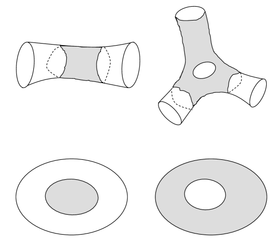
Figure 1. Four examples: $E_{i}$ (shadow region) is parallel to $S_{i}$. $p_{i},q_{i}$ are marked points in $P$. Here, $S_{1}$ is an annulus with one marked point, $S_{2}$ has three boundary curves and contains no marked point, both $S_{3}$ and $S_{4}$ are disks with two marked points.

Note that if $T$ is parallel to $S$ and $A$ is an annular component of $S\setminus T$, then one boundary curve of $A$ is on $S$. Moreover, $\#(T\cap P)+\#\partial(T)\geq\#(S\cap P)+\#\partial(S)\geq 3$.

Here is an important property of the $\mathcal{S}$-pieces:

Lemma 3.4.

For every $\mathcal{S}$-piece $S$, there is a unique $\mathcal{E}$-piece parallel to $S$.

Proof.

Let $\mathcal{C}_{1}$ be the collection of all curves of $f^{-1}(\Sigma)$, contained in the interior of $S$ and non peripheral in $\mathbb{\overline{C}}-P$. Since $\Gamma$ is $(f,P)$-stable, each curve $\gamma\in\mathcal{C}_{1}$ is homotopic in $\mathbb{\overline{C}}-P$ to exactly one boundary curve, say $\tau_{\gamma}$, of $S$. Let $A(\gamma)$ be the open annulus bounded by $\gamma$ and $\tau_{\gamma}$. Since distinct curves in $f^{-1}(\Sigma)$ are disjoint, we conclude that for any two curves $\gamma_{1},\gamma_{2}\in\mathcal{C}_{1}$, the annuli $A(\gamma_{1})$ and $A(\gamma_{2})$ either are disjoint or one contains another. Thus $\cup_{\gamma\in\mathcal{C}_{1}}A(\gamma)$ consists of finitely many annular components.

Let $\mathcal{C}_{2}$ be the collection of all curves of $f^{-1}(\Sigma)$, contained in $S-\cup_{\gamma\in\mathcal{C}_{1}}(A(\gamma)\cup\tau_{\gamma})$, peripheral or null homotopic in $\mathbb{\overline{C}}-P$. Then each curve $\alpha\in\mathcal{C}_{2}$ bounds an open disk $D(\alpha)\subset S$. Moreover, for any two curves $\alpha_{1},\alpha_{2}\in\mathcal{C}_{2}$, the disks $D(\alpha_{1})$ and $D(\alpha_{2})$ either are disjoint or one contains another. Thus $\cup_{\alpha\in\mathcal{C}_{2}}D(\alpha)$ consists of finitely many disk components.

The set $E_{S}:=S-\cup_{\gamma\in\mathcal{C}_{1}}(A(\gamma)\cup\tau_{\gamma})-\cup_{\alpha\in\mathcal{C}_{2}}D(\alpha)$ is a closed and non-empty set. It is connected since each component of $\mathbb{\overline{C}}-E_{S}$ is a disk. The interior of $E_{S}$ contains no curve of $f^{-1}(\Sigma)$, thus it is an $\mathcal{{E}}$-piece. It is in fact the unique $\mathcal{{E}}$-piece parallel to $S$ by construction. ∎

See Figure 1 for the examples of ‘parallel’ pieces. In the following discussion, we always use $E_{S}$ to denote the $\mathcal{E}$-piece parallel to $S$.

Based on Lemma 3.4, we see that $(f,P)$ induces a well-defined map $f_{*}$ from $\mathcal{S}$ to itself:

$$f_{*}:\mathcal{S}\ni S\mapsto f(E_{S})\in\mathcal{S}.$$

Since there are finitely many $\mathcal{S}$-pieces, every $\mathcal{S}$-piece is pre-periodic.

For each curve $\gamma\in\partial(S)$, there is a unique boundary curve $\beta_{\gamma}\in\partial(E_{S})$ such that either $\beta_{\gamma}=\gamma$, or $\beta_{\gamma}$ and $\gamma$ bound an annulus in $S-P$. We define three sets $\partial_{0}(S),\partial_{1}(S),\partial_{2}(S)$ as follows:

$$\partial_{0}(S) = \{\gamma\in\partial(S);\gamma\in\Gamma_{0}\},$$

$$\partial_{1}(S) = \{\gamma\in\partial(S);\gamma\neq\beta_{\gamma}\},$$

$$\partial_{2}(S) = \{\gamma\in\partial(S);\gamma=\beta_{\gamma}\}-\Gamma_{0}.$$

Lemma 3.5.

If $\partial_{0}(S)\neq\emptyset$, then we have:

1. For any $\gamma\in\partial_{0}(S)$, $\gamma=\beta_{\gamma}$.

2. $S$ is $f_{*}$-periodic.

3. $\#\partial_{0}(S)=\#\partial_{0}(f_{*}(S))$.

Proof.

1. Note that each component of $S-E_{S}$ is either a disk containing at most one point in $P$, or an annulus in $\mathbb{\overline{C}}-P$. It follows that if $\gamma\in\partial_{0}(S)$, then $\gamma\subset P$ and $\gamma=\beta_{\gamma}$.

2. Take a curve $\gamma\in\partial_{0}(S)$ and let $A_{\gamma}\in\mathcal{A}$ be the rotation annulus containing $\gamma$. Then from 1 we see that $S\cap A_{\gamma}=E_{S}\cap A_{\gamma}$. This implies $f(S\cap A_{\gamma})=f_{*}(S)\cap f(A_{\gamma})$. Let $k\geq 1$ be the period of $A_{\gamma}$. Then we have $S\cap A_{\gamma}=f^{k}(S\cap A_{\gamma})=f^{k}_{*}(S)\cap f^{k}(A_{\gamma})=f^{k}_{*}(S)\cap A_{\gamma}$. Thus $f^{k}_{*}(S)=S$ and the period of $S$ is a divisor of $k$.

3. It follows from 1 that if $\gamma\in\partial_{0}(S)$, then $f(\gamma)\in\partial_{0}(f_{*}(S))$. So $\#\partial_{0}(S)\leq\#\partial_{0}(f_{*}(S))\leq\cdots$. Since $S$ is $f_{*}$-periodic (by 2), we have $\#\partial_{0}(S)=\#\partial_{0}(f_{*}(S))$. ∎

It follows from Lemma 3.5 that $\partial_{i}(S),i\in\{0,1,2\}$ are mutually disjoint and $\partial(S)=\partial_{0}(S)\sqcup\partial_{1}(S)\sqcup\partial_{2}(S)$.

Remark 3.6.

Suppose $\partial_{0}(S)\neq\emptyset$. For each $\gamma\in\partial_{0}(S)$, let ${\rm per}(\gamma)$ be the period of $\gamma$. From Lemma 3.5 we see that the $f_{*}$-period of $S$ is a devisor of ${\rm gcd}\{{\rm per}(\gamma);\gamma\in\partial_{0}(S)\}$. In particular, if ${\rm gcd}\{{\rm per}(\gamma);\gamma\in\partial_{0}(S)\}=1$, then $f_{*}(S)=S$ and for any $\gamma\in\partial_{0}(S)$ and any $k\geq 0$, we have $f^{k}(\gamma)\in\partial_{0}(S)$.

For example, suppose that $(f,P)$ has two cycles of rotation annuli whose periods are different prime numbers, say $p$ and $q$. If $\partial_{0}(S)\neq\emptyset$, then $\#\partial_{0}(S)$ takes only four possible values: 1, $p$, $q$ and $p+q$.

3.2. Marked disk extension

For each $\mathcal{S}$-piece $S$, we denote by $\mathbb{\overline{C}}(S)$ the Riemann sphere containing $S$. We always consider that different $\mathcal{S}$-pieces are embedded into different copies of Riemann spheres.

In the following, we will extend $f|_{E_{S}}$ to a branched covering $H_{S}:\mathbb{\overline{C}}(S)\rightarrow\mathbb{\overline{C}}(f_{*}(S))$ with $\deg(H_{S})=\deg(f|_{E_{S}})$. The extension is canonical and unique up to c-equivalence. If $f$ is quasi-regular, we may also require $H_{S}$ is quasi-regular. To do this, we need to define the map $H_{S}:\mathbb{\overline{C}}(S)-E_{S}\rightarrow\mathbb{\overline{C}}(f_{*}(S))-f_{*}(S)$ such that $H_{S}|_{\partial E_{S}}=f|_{\partial E_{S}}$. We will define $H_{S}$ component by component.

Note that each component of $\mathbb{\overline{C}}(S)-E_{S}$ is a disk. Let $U$ be such a component with boundary curve $\gamma$.

We first deal with the case when $\gamma\in\partial_{0}(S)$. In this case, there is a rotation annulus $A_{\gamma}$ containing $\gamma$. Let $k\geq 1$ be the period of $A_{\gamma}$ and $\phi_{0}:S\cap A_{\gamma}\rightarrow\mathbb{A}_{R}:=\{z\in\mathbb{C};1<|z|<R\}$ be the conformal map such that $\phi_{0}f^{k}\phi^{-1}_{0}(z)=e^{2\pi i\theta}z$ for $z\in\mathbb{A}_{R}$. For $1\leq j\leq k-1$, we define a conformal map from $f^{j}(S\cap A_{\gamma})$ onto $\mathbb{A}_{R}$ by $\phi_{j}=\phi_{0}f^{k-j}|_{f^{j}(S\cap A_{\gamma})}$. Then we have the following commutative diagram

Let $\mathbb{D}_{R}=\{z\in\mathbb{C};|z|<R\}$. For $0\leq j<k$, we consider the disk $\Delta_{j}$ obtained by gluing $f^{j}(S\cap A_{\gamma})$ and $\mathbb{D}_{R}$ via the map $\phi_{j}$. The disk $\Delta_{j}$ inherits a natural complex structure from $\mathbb{D}_{R}$ since $\phi_{j}$ is holomorphic.

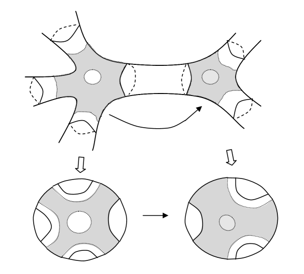
Figure 2. Marked disk extension. Here $\partial S=\gamma_{1}\cup\gamma_{2}\cup\gamma_{3}\cup\gamma_{4}$, $\partial f_{*}(S)=\gamma_{5}\cup\gamma_{6}\cup\gamma_{7}$. Marked points are labeled by ‘$\bullet$’.

The map $H_{f_{*}^{j}(S)}:\Delta_{j}\rightarrow\Delta_{j+1}$ defined by

$$H_{f_{*}^{j}(S)}(z)=\begin{cases}f(z),\ \ &z\in f^{j}(S\cap A_{\gamma}),\ 0\leq j<k,\\ e^{2\pi i\theta}z,\ \ &z\in\mathbb{D},\ j=0,\\ z,\ \ &z\in\mathbb{D},\ 1\leq j<k.\end{cases}$$

is a holomorphic extension of $f|_{E_{f_{*}^{j}(S)}}$ along the boundary curve $f^{j}(\gamma)\in\partial_{0}(f_{*}^{j}(S))$. We call $\Delta_{j}$ a holomorphic disk of $H_{f_{*}^{j}(S)}$. This construction allows us to define the extensions of $f|_{E_{S}},\cdots,f|_{E_{f_{*}^{l-1}(S)}}$ (where $l$ is the $f_{*}$-period of $S$) along the curves in $\partial_{0}(S)\cup\cdots\cup\partial_{0}(f_{*}^{l-1}(S))$ at the same time. We denote by $\Delta_{j}^{0}\subset\Delta_{j}$ the sub-disk of $\Delta_{j}$ with boundary curve $f^{j}(\gamma)$, $0_{j}$ the center of $\Delta_{j}$. In this case, we get a marked disk $(\Delta_{j}^{0},0_{j})$.

Now, we consider the case when $\gamma\in\partial(E_{S})\setminus\partial_{0}(S)$. Note that either $U\subset S$ and $U$ contains at most one point in $P$, or $U$ contains exactly one component $V$ of $\mathbb{\overline{C}}(S)-S$. In the former case, if $U$ contains a marked point $p\in P$, then we get a marked disk $(U,p)$; if $U\cap P=\emptyset$, then we don’t mark any point in $U$. In the latter case, we mark a point $p\in V$ and get two marked disks $(U,p)$ and $(V,p)$.

Now we extend $f|_{E_{S}}$ to $U$ in the following fashion:

We require that $H_{S}$ maps $U$ onto $(W,q)$ with $\deg(H_{S}|_{U})=\deg(f|_{\partial U})$, where $(W,q)$ is the marked disk of $\mathbb{\overline{C}}(f_{*}(S))-f_{*}(S)$ whose boundary curve is $f(\partial U)$. If $U$ contains a marked point $p$, we require further $H(p)=q$ and the local degree of $H_{S}$ at $p$ is equal to $\deg(f|_{\partial U})$. If $U$ contains no marked point, we require that $q$ is the only possible critical value (this implies that $U$ contains at most one ramification point of $H_{S}$).

In this way, for each $\mathcal{S}$-piece $S$, we can get an extension $H_{S}:\mathbb{\overline{C}}(S)\rightarrow\mathbb{\overline{C}}(f_{*}(S))$ of $f|_{E_{S}}$. Let $Z(S)=\{p;(V,p)\text{ is a marked disk in }\mathbb{\overline{C}}(S)-S\}$, ${D}(S)$ be the union of all holomorphic disks of $H_{S}$. Note that if $\partial_{0}(S)=\emptyset$, then ${D}(S)=\emptyset$. Set

$$P(S)=(P\cap S)\cup Z(S)\cup{D}(S).$$

We call $(\mathbb{\overline{C}}(S),P(S))$ a marked sphere of $\mathbb{\overline{C}}(S)$. By the construction of $H_{S}$, we see that $H_{S}(P(S))\subset P(f_{*}(S))$.

We know that every $\mathcal{S}$-piece is eventually periodic under the map $f_{*}$. Let $n$ be the number of all $f_{*}$-cycles of $\mathcal{S}$-pieces. These cycles are listed as follows:

$$S_{\nu}\mapsto f_{*}(S_{\nu})\mapsto\cdots\mapsto f_{*}^{p_{\nu}-1}(S_{\nu})\mapsto f_{*}^{p_{\nu}}(S_{\nu})=S_{\nu},\ \ 1\leq\nu\leq n,$$

where $S_{\nu}$ is a representative of the $\nu$-th cycle and $p_{\nu}$ is the period of $S_{\nu}$.

Set

$$h_{\nu}=H_{f_{*}^{p_{\nu}-1}(S_{\nu})}\circ\cdots\circ H_{f_{*}(S_{\nu})}\circ H_{S_{\nu}},\ P_{\nu}=P(S_{\nu}),\ \ 1\leq\nu\leq n.$$

Then $h_{\nu}:\mathbb{\overline{C}}(S_{\nu})\rightarrow\mathbb{\overline{C}}(S_{\nu})$ is a branched covering with $h_{\nu}(P_{\nu})\subset P_{\nu}$.

These resulting maps $(h_{1},P_{1}),\cdots,(h_{n},P_{n})$ can be considered as the renormalizations of the original map $(f,P)$. There are three types of them:

$\bullet$ $\partial_{0}(S_{\nu})\neq\emptyset$ or $S_{\nu}$ contains at least one rotation disk of $(f,P)$. In this case, $(h_{\nu},P_{\nu})$ has at least one cycle of rotation disks, so $(h_{\nu},P_{\nu})$ is a Siegel map. Moreover, a curve $\gamma\in\partial_{0}(S_{\nu})$ in a rotation annulus of $(f,P)$ with period $p$ and rotation number $\theta$ becomes a periodic curve in a rotation disk of $(h_{\nu},P_{\nu})$, with period $p/p_{\nu}$ and rotation number $\theta$. One may verify that the number of these resulting Siegel maps is at least two, and at most $2n_{RA}(f)+n_{RD}(f)$.

$\bullet$ $\partial_{0}(S_{\nu})=\emptyset$, $S_{\nu}$ contains no rotation disk of $(f,P)$ and $\deg(h_{\nu})>1$. In this case, $P_{\nu}$ is a finite set and $(h_{\nu},P_{\nu})$ is a Thurston map.

$\bullet$ $\partial_{0}(S_{\nu})=\emptyset$, $S_{\nu}$ contains no rotation disk of $(f,P)$ and $\deg(h_{\nu})=1$. In this case, $(h_{\nu},P_{\nu})$ is a homeomorphism of $\mathbb{\overline{C}}(S_{\nu})$ and $h_{\nu}(P_{\nu})=P_{\nu}$. So every point of $P_{\nu}$ is periodic. Moreover, for any $S\in\{S_{\nu},f_{*}(S_{\nu}),\cdots,f_{*}^{p_{\nu}-1}(S_{\nu})\}$, each component of $S-E_{S}$ is an annulus.

Let $\Lambda$ be the index set consisting of all $\nu\in\{1,\cdots,n\}$ such that $\deg(h_{\nu})>1$. That is, for each $\nu\in\Lambda$, $(h_{\nu},P_{\nu})$ is either a Siegel map or a Thurston map. Let $\Lambda^{*}=\{1,\cdots,n\}-\Lambda$.

We use the following notation to record the above decomposition and marked disk extension procedure:

$${\rm Dec}(f,P)=\Bigg{(}\bigoplus_{\nu\in\Lambda\cup\Lambda^{*}}(h_{\nu},P_{\nu})\Bigg{)}_{\Gamma}.$$

Lemma 3.7.

If $\lambda(\Gamma,f)<1$, then

1. For any $1\leq\nu\leq n$, every point in $Z(S_{\nu})$ is eventually mapped to either the center of some rotation disk or a periodic critical point of $(h_{\nu},P_{\nu})$.

2. $\Lambda^{*}=\emptyset$.

3. If $(h_{\nu},P_{\nu})$ is a Thurston map, then the signature of the orbifold of $(h_{\nu},P_{\nu})$ is not $(2,2,2,2)$.

Proof.

Since $h_{\nu}(Z(S_{\nu}))\subset Z(S_{\nu})$ and $Z(S_{\nu})$ is a finite set, we conclude that every point in $Z(S_{\nu})$ is eventually periodic under the iterations of $(h_{\nu},P_{\nu})$.

If $\Gamma=\emptyset$, then $\partial(S_{\nu})\subset\Gamma_{0}$ and all resulting maps $(h_{\nu},P_{\nu})$ are Siegel maps. The marked disk extension procedure implies that every point in $Z(S_{\nu})$ is the center of some rotation disk. The conclusions follows immediately in this case.

In the following, we assume $\Gamma\neq\emptyset$. Let $z_{0}$ be a periodic point in $Z(S_{\nu})$ with period $k$. Suppose that $z_{0}$ is not the center of any rotation disk, and let $\beta$ be the boundary curve of $S_{\nu}$ that encloses $z_{0}$. Then there is a unique component of $h_{\nu}^{-k}(\beta)$, say $\alpha$, contained in $S_{\nu}$ and homotopic to $\beta$ in $\mathbb{\overline{C}}(S_{\nu})-P_{\nu}$. Thus

$${\rm deg}(h_{\nu}^{k},z_{0})={\rm deg}(h_{\nu}^{k}:\alpha\rightarrow\beta)={\rm deg}(f^{kp_{\nu}}:\alpha\rightarrow\beta)\geq\lambda(\Gamma,f)^{-kp_{\nu}}>1.$$

This implies that $z_{0}$ lies in a critical cycle and $\deg(h_{\nu})>1$. It follows that $\Lambda^{*}=\emptyset$ and there is no $(2,2,2,2)$-type Thurston map among $(h_{\nu},P_{\nu})_{\nu\in\Lambda}$. ∎

4. Combination part: decompositions of stable multicurve

In this section, we will prove the following:

Theorem 4.1.

Let $(f,P)$ be a Herman map, and

$${\rm Dec}(f,P)=\Bigg{(}\bigoplus_{\nu\in\Lambda\cup\Lambda^{*}}(h_{\nu},P_{\nu})\Bigg{)}_{\Gamma}.$$

Then $(f,P)$ has no Thurston obstructions if and only if $\lambda(\Gamma,f)<1$ and for each $\nu\in\Lambda$, $(h_{\nu},P_{\nu})$ has no Thurston obstructions.

Note that if $(f,P)$ has no Thurston obstructions or $\lambda(\Gamma,f)<1$, then $\Lambda^{*}=\emptyset$ (see Lemma 3.7).

The proof of the ‘sufficiency’ of Theorem 4.1 is based on the decomposition of $(f,P)$-stable multicurves. We will show that every $(f,P)$-stable multicurve contains an ‘essential’ submulticurve (Lemma 4.2), and every such essential submulticurve can be decomposed into a ‘$\Gamma$-part’ multicurve together with a $(h_{\nu},P_{\nu})$-stable multicurve for each $\nu\in[1,n]$. The important fact of this decomposition is that the leading eigenvalues of the transition matrices satisfy the so-called ‘reduction identity’ (Theorem 4.3).

To prove the ‘necessity’ of Theorem 4.1, we will show that every $(h_{\nu},P_{\nu})$-stable multicurve $\Sigma$ can generate a $(f,P)$-stable multicurve $\mathcal{C}$ with $\lambda(\Sigma,h_{\nu})\leq\lambda(\mathcal{C},f)^{p_{\nu}}$.

Lemma 4.2 (‘Essential’ submulticurve).

Let $\mathcal{C}_{0}$ be a $(f,P)$-stable multicurve, then there is a $(f,P)$-stable multicurve $\mathcal{C}$, such that

1. $\mathcal{C}$ is homotopically contained in $\mathcal{C}_{0}$.

2. Each curve of $\mathcal{C}$ is contained in the interior of some $\mathcal{S}$-piece.

3. $\lambda(\mathcal{C},f)=\lambda(\mathcal{C}_{0},f)$.

Proof.

For $n\geq 1$, we define a multicurve $\mathcal{C}_{n}$ inductively: $\mathcal{C}_{n}\subset f^{-1}(\mathcal{C}_{n-1})$ and $\mathcal{C}_{n}$ represents all homotopy classes of non-peripheral curves of $f^{-1}(\mathcal{C}_{n-1})$. Since $\mathcal{C}_{0}$ is a $(f,P)$-stable multicurve, we conclude that all $\mathcal{C}_{n}$ are $(f,P)$-stable, and $\mathcal{C}_{n}$ is homotopically contained in $\mathcal{C}_{n-1}$. Let $W_{n}$ be the $(f,P)$-transition matrix of $\mathcal{C}_{n}$ for $n\geq 0$, then

$$W_{n}=\left(\begin{array}[]{cc}W_{n+1}&*\\ O&O\end{array}\right).$$

Thus $\lambda(\mathcal{C}_{0},f)=\lambda(\mathcal{C}_{1},f)=\lambda(\mathcal{C}_{2},f)=\cdots$. By the construction of $\Gamma$, there is an integer $N\geq 0$ such that $\Gamma\subset f^{-n}(\Gamma_{0})$ for all $n\geq N$, where $\Gamma_{0}$ is the choice of a collection of $f$-periodic curves in the rotation annuli (see the previous section). Since $\cup\Gamma_{0}$ has no intersection with $\cup\mathcal{C}_{0}$, we conclude that $f^{-n}(\cup\Gamma_{0})$ has no intersection with $f^{-n}(\cup\mathcal{C}_{0})$ for all $n\geq 1$. Thus when $n\geq N$, we have $\cup\mathcal{C}_{n}\subset f^{-n}(\cup\mathcal{C}_{0})\subset\mathbb{\overline{C}}\setminus f^{-n}(\cup\Gamma_{0})\subset\mathbb{\overline{C}}\setminus\cup(\Gamma\cup\Gamma_{0})$. This implies that each curve of $\mathcal{C}_{n}$ is contained in the interior of some $\mathcal{S}$-piece. The proof is completed if we set $\mathcal{C}=\mathcal{C}_{n}$ for some $n\geq N$. ∎

Theorem 4.3 (Decomposition of stable multicurve).

Let $\mathcal{C}$ be a $(f,P)$-stable multicurve. Suppose that each curve of $\mathcal{C}$ is contained in the interior of some $\mathcal{S}$-piece. Let

$$\mathcal{C}_{\Gamma}=\{\gamma\in\mathcal{C};\gamma\text{ is homotopic in }\mathbb{\overline{C}}-P\text{ to a curve of }\Gamma\},$$

$$\Sigma_{\nu}=\{\gamma\in\mathcal{C}-\mathcal{C}_{\Gamma};\gamma\text{ is contained in }S_{\nu}\},\ \nu\in\Lambda\cup\Lambda^{*}=[1,n].$$

Then $\mathcal{C}_{\Gamma}$ is a $(f,P)$-stable multicurve, $\Sigma_{\nu}$ is a $(h_{\nu},P_{\nu})$-stable multicurve for each $\nu\in[1,n]$, and we have the following reduction identity:

$$\lambda(\mathcal{C},f)=\max\Big{\{}\lambda(\mathcal{C}_{\Gamma},f),\sqrt[p_{1}]{\lambda(\Sigma_{1},h_{1})},\cdots,\sqrt[p_{n}]{\lambda(\Sigma_{n},h_{n})}\Big{\}}.$$

Remark 4.4.

In Theorem 4.3, the multicurve $\Sigma_{\nu}$ can be viewed as a multicurve of $(h_{\nu},P_{\nu})$, this is because under the inclusion map $\iota_{\nu}:S_{\nu}\hookrightarrow\mathbb{\overline{C}}(S_{\nu})$, the set $\iota_{\nu}(\Sigma_{\nu}):=\{\iota_{\nu}(\gamma);\gamma\in\Sigma_{\nu}\}$ is a multicurve in $\mathbb{\overline{C}}(S_{\nu})-P_{\nu}$. We still use $\Sigma_{\nu}$ to denote the multicurve $\iota_{\nu}(\Sigma_{\nu})$ if there is no confusion.

One may show directly that if $\Lambda^{*}\neq\emptyset$, then for any $\nu\in\Lambda^{*}$,

$$\lambda(\Sigma_{\nu},h_{\nu})=\begin{cases}1,&\text{ if }\Sigma_{\nu}\neq\emptyset,\\ 0,&\text{ if }\Sigma_{\nu}=\emptyset.\end{cases}$$

This observation can simplify the reduction identity.

Proof.

The fact that $\mathcal{C}_{\Gamma}$ is $(f,P)$-stable is easy to verify since both $\Gamma$ and $\mathcal{C}$ are $(f,P)$-stable. Let $\Sigma_{\nu}^{k}=\{\gamma\in\mathcal{C}-\mathcal{C}_{\Gamma};\gamma\text{ is contained in }f^{k}_{*}(S_{\nu})\}$ for $0\leq k\leq p_{\nu}$. It’s obvious that $\Sigma_{\nu}^{0}=\Sigma_{\nu}^{p_{\nu}}=\Sigma_{\nu}$. Since $\mathcal{C}$ is $(f,P)$-stable, each non-peripheral component of $f^{-1}(\gamma)$ for $\gamma\in\Sigma_{\nu}^{k+1}(0\leq k<p_{\nu})$ is homotopic in $\mathbb{\overline{C}}-P$ to either a curve $\alpha\in\mathcal{C}_{\Gamma}$, or a curve $\beta\in\Sigma_{\nu}^{k}$, or a curve $\delta$ contained in a strictly preperiodic $\mathcal{S}$-piece.

By the definition of the marked set $P(f^{k}_{*}(S_{\nu}))$, one can verify that the set $\Sigma_{\nu}^{k}$ is a multicurve in $\mathbb{\overline{C}}(f^{k}_{*}(S_{\nu}))-P(f^{k}_{*}(S_{\nu}))$. Moreover, each curve $\gamma\in\mathcal{C}_{\Gamma}$ contained in $f^{k}_{*}(S_{\nu})$ is peripheral or null-homotopic in $\mathbb{\overline{C}}(f^{k}_{*}(S_{\nu}))-P(f^{k}_{*}(S_{\nu}))$. Thus for any $0\leq k<p_{\nu}$ and any curve $\gamma\in\Sigma_{\nu}^{k+1}$, each non-peripheral component of $H_{f^{k}_{*}(S_{\nu})}^{-1}(\gamma)$ is homotopic to a curve $\delta\in\Sigma_{\nu}^{k}$ in $\mathbb{\overline{C}}(f^{k}_{*}(S_{\nu}))-P(f^{k}_{*}(S_{\nu}))$. It follows that each non-peripheral component of $h_{\nu}^{-1}(\gamma)$ with $\gamma\in\Sigma_{\nu}$ is homotopic to a curve $\delta\in\Sigma_{\nu}$ in $\mathbb{\overline{C}}(S_{\nu})-P_{\nu}$. This means $\Sigma_{\nu}$ is a $(h_{\nu},P_{\nu})$-stable multicurve.

In the following, we will prove the ‘reduction identity’. Let $W_{\mathcal{C}_{\Gamma}}$ be the $(f,P)$-transition matrix of $\mathcal{C}_{\Gamma}$. We define $\mathcal{C}_{s}:=\{\gamma\in\mathcal{C}-\mathcal{C}_{\Gamma};\gamma\text{ is contained in}$ $\text{a strictly preperiodic }\mathcal{S}\text{-piece}\}$ with $(f,P)$-transition matrix $W_{s}$. Let $\mathcal{C}_{\nu}=\Sigma_{\nu}^{0}\cup\cdots\cup\Sigma_{\nu}^{p_{\nu}-1}$ with $(f,P)$-transition matrix $W_{\nu}$. Then the $(f,P)$-transition matrix $W_{\mathcal{C}}$ of $\mathcal{C}$ has the following block decomposition:

$$W_{\mathcal{C}}=\left(\begin{array}[]{ccccc}W_{\mathcal{C}_{\Gamma}}&*&*&\cdots&*\\ O&W_{s}&*&\cdots&*\\ O&O&W_{1}&\cdots&*\\ \vdots&\vdots&\vdots&\ddots&\vdots\\ O&O&O&\cdots&W_{n}\end{array}\right).$$

It follows that $\lambda(\mathcal{C},f)=\max\big{\{}\lambda(\mathcal{C}_{\Gamma},f),\lambda(\mathcal{C}_{s},f),\lambda(\mathcal{C}_{1},f),\cdots,\lambda(\mathcal{C}_{n},f)\big{\}}$.

We claim that $\lambda(\mathcal{C}_{s},f)=0$. To see this, let $\mathcal{S}_{s}$ be the collection of all strictly preperiodic $\mathcal{S}$-pieces. For each $S\in\mathcal{S}_{s}$, let $\tau(S)$ be the least integer $k\geq 1$ such that $f_{*}^{k}(S)$ is a periodic $\mathcal{S}$-piece. Set $M=\max\{\tau(S);S\in\mathcal{S}_{s}\}$. For any $\gamma\in\mathcal{C}_{s}$, let $\alpha$ be a non-peripheral component of $f^{-M}(\gamma)$. If $\alpha$ is not homotopic to any curve in $\mathcal{C}_{\Gamma}$, then there is $S_{\alpha}\in\mathcal{S}_{s}$ such that $\alpha$ is contained in the $\mathcal{E}$-piece $E_{S_{\alpha}}$ parallel to $S_{\alpha}$. Moreover, for any $1\leq j<M$, $f^{j}(\alpha)$ is not homotopic to any curve in $\mathcal{C}_{\Gamma}$ and $f^{j}(\alpha)\subset E_{f^{j}_{*}(S_{\alpha})}$. In particular, $f^{M}(\alpha)=\gamma\subset f^{M}_{*}(S_{\alpha})\in\mathcal{S}_{s}$. This implies $\tau(S_{\alpha})\geq M+1$. But this contradicts the choice of $M$. Thus, $\alpha$ is either null-homotopic, or peripheral, or homotopic to a curve $\delta\in\mathcal{C}_{\Gamma}$ in $\mathbb{\overline{C}}-P$. Equivalently, $W^{M}_{s}=0$ and $\lambda(\mathcal{C}_{s},f)=0$. So we have

$$\lambda(\mathcal{C},f)=\max\Big{\{}\lambda(\mathcal{C}_{\Gamma},f),\lambda(\mathcal{C}_{1},f),\cdots,\lambda(\mathcal{C}_{n},f)\Big{\}}.$$

Notice that the $(f,P)$-transition matrix $W_{\nu}$ of $\mathcal{C}_{\nu}$ takes the form

$$W_{\nu}=\left(\begin{array}[]{ccccc}O&B_{0}&O&\cdots&O\\ O&O&B_{1}&\cdots&O\\ \vdots&\vdots&\vdots&\ddots&\vdots\\ O&O&O&\cdots&B_{p_{\nu}-2}\\ B_{p_{\nu}-1}&O&O&\cdots&O\end{array}\right),$$

where $B_{j}$ is a $n_{j}\times n_{j+1}$ matrix, $n_{j}$ is equal to the number of curves in $\Sigma_{\nu}^{j}$ for $0\leq j\leq p_{\nu}-1$. A direct calculation yields

$$W^{p_{\nu}}_{\nu}=\left(\begin{array}[]{ccccc}B_{0}B_{1}\cdots B_{p_{\nu}-1}&O&\cdots&O\\ O&B_{1}B_{2}\cdots B_{0}&\cdots&O\\ \vdots&\vdots&\ddots&\vdots\\ O&O&\cdots&B_{p_{\nu}-1}B_{0}\cdots B_{p_{\nu}-2}\end{array}\right).$$

For any $k\geq 1$, we have

$$\|(W_{\nu}^{p_{\nu}})^{k}\|^{2}=\|(B_{0}B_{1}\cdots B_{p_{\nu}-1})^{k}\|^{2}+\cdots+\|(B_{p_{\nu}-1}B_{0}\cdots B_{p_{\nu}-2})^{k}\|^{2}.$$

It follows from Lemma 4.5 that

$$\mathrm{sp}(W_{\nu})^{p_{\nu}}=\mathrm{sp}(B_{0}B_{1}\cdots B_{p_{\nu}-1})=\cdots=\mathrm{sp}(B_{p_{\nu}-1}B_{0}\cdots B_{p_{\nu}-2}).$$

On the other hand, one can verify that the $(h_{\nu},P_{\nu})$-transition matrix of $\Sigma_{\nu}$ is $B_{0}B_{1}\cdots B_{p_{\nu}-1}$. It follows from Perron-Frobenius Theorem that

$$\lambda(\Sigma_{\nu},h_{\nu})=\mathrm{sp}(B_{0}B_{1}\cdots B_{p_{\nu}-1})=\mathrm{sp}(W_{\nu})^{p_{\nu}}=\lambda(\mathcal{C}_{\nu},f)^{p_{\nu}}.$$

Finally, we get the reduction identity

$$\lambda(\mathcal{C},f) = \max\Big{\{}\lambda(\mathcal{C}_{\Gamma},f),\sqrt[p_{1}]{\lambda(\Sigma_{1},h_{1})},\cdots,\sqrt[p_{n}]{\lambda(\Sigma_{n},h_{n})}\Big{\}}.$$

∎

Lemma 4.5.

Let $B_{\nu}$ be a $n_{\nu}\times n_{\nu+1}$ real matrix for $1\leq\nu\leq k$, $n_{k+1}=n_{1}$, then

$$\mathrm{sp}(B_{1}B_{2}\cdots B_{k})=\mathrm{sp}(B_{2}B_{3}\cdots B_{1})=\cdots=\mathrm{sp}(B_{k}B_{1}\cdots B_{k-1}).$$

Proof.

First we assume $n_{1}=\cdots=n_{k}$, fix some $1\leq\nu\leq k$, by Cauchy-Schwarz inequality (i.e. $\|AB\|\leq\|A\|\|B\|$),

$$\mathrm{sp}(B_{1}B_{2}\cdots B_{k}) = \lim_{n\rightarrow\infty}\sqrt[n]{\|(B_{1}B_{2}\cdots B_{k})^{n}\|}$$

$$= \lim_{n\rightarrow\infty}\sqrt[n]{\|(B_{1}\cdots B_{\nu-1})(B_{\nu}B_{\nu+1}\cdots B_{\nu-1})^{n-1}(B_{\nu}\cdots B_{k})\|}$$

$$\leq \lim_{n\rightarrow\infty}\sqrt[n]{\|B_{1}\cdots B_{\nu-1}\|\|(B_{\nu}B_{\nu+1}\cdots B_{\nu-1})^{n-1}\|\|B_{\nu}\cdots B_{k}\|}$$

$$= \mathrm{sp}(B_{\nu}B_{\nu+1}\cdots B_{\nu-1}).$$

The same argument leads to the other direction of the inequality. In the following, we deal with the general case. Choose $n\geq\max\{n_{1},\cdots,n_{k}\}$, for any $1\leq\nu\leq k$, we define a $n\times n$ matrix $\widehat{B}_{\nu}$ by

$$\widehat{B}_{\nu}=\left(\begin{array}[]{cc}{B}_{\nu}&O_{n_{\nu}\times(n-n_{\nu+1})}\\ O_{(n-n_{\nu})\times n_{\nu+1}}&O_{(n-n_{\nu})\times(n-n_{\nu+1})}\end{array}\right),$$

where we use $O_{p\times q}$ to denote the $p\times q$ zero matrix. Then by the above argument, $\mathrm{sp}(\widehat{B}_{1}\widehat{B}_{2}\cdots\widehat{B}_{k})=\mathrm{sp}(\widehat{B}_{\nu}\widehat{B}_{\nu+1}\cdots\widehat{B}_{\nu-1}).$ On the other hand,

$$\widehat{B}_{\nu}\widehat{B}_{\nu+1}\cdots\widehat{B}_{\nu-1}=\left(\begin{array}[]{cc}B_{\nu}B_{\nu+1}\cdots B_{\nu-1}&O_{n_{\nu}\times(n-n_{\nu})}\\ O_{(n-n_{\nu})\times n_{\nu}}&O_{(n-n_{\nu})\times(n-n_{\nu})}\end{array}\right).$$

This implies that $\|(B_{1}B_{2}\cdots B_{k})^{n}\|=\|(\widehat{B}_{1}\widehat{B}_{2}\cdots\widehat{B}_{k})^{n}\|$ for all $n\geq 1$. So

$$\mathrm{sp}(B_{1}\cdots B_{k})=\mathrm{sp}(\widehat{B}_{1}\cdots\widehat{B}_{k})=\mathrm{sp}(\widehat{B}_{\nu}\cdots\widehat{B}_{\nu-1})=\mathrm{sp}(B_{\nu}\cdots B_{\nu-1}).$$

∎

Proof of Theorem 4.1. Sufficiency. Let $\mathcal{C}$ be a $(f,P)$-stable multicurve in $\mathbb{\overline{C}}-P$. We may assume that each curve $\gamma\in\mathcal{C}$ is contained in the interior of some $\mathcal{S}$-piece by Lemma 4.2. The multicurves $\mathcal{C}_{\Gamma},\Sigma_{1},\cdots,\Sigma_{n}$ are the subsets of $\mathcal{C}$ defined in Theorem 4.3. If $\lambda(\Gamma,f)<1$ (note that this implies $\Lambda^{*}=\emptyset$ by Lemma 3.7) and $(h_{\nu},P_{\nu})$ has no Thurston obstructions for each $\nu\in\Lambda$, then by Theorem 4.3, we have

$$\lambda(\mathcal{C},f) = \max\Big{\{}\lambda(\mathcal{C}_{\Gamma},f),\sqrt[p_{1}]{\lambda(\Sigma_{1},h_{1})},\cdots,\sqrt[p_{n}]{\lambda(\Sigma_{n},h_{n})}\Big{\}}$$

$$\leq \max\Big{\{}\lambda(\Gamma,f),\sqrt[p_{1}]{\lambda(\Sigma_{1},h_{1})},\cdots,\sqrt[p_{n}]{\lambda(\Sigma_{n},h_{n})}\Big{\}}<1.$$

This means $(f,P)$ has no Thurston obstructions.

Necessity. Suppose that $(f,P)$ has no Thurston obstructions. Then $\lambda(\Gamma,f)<1$ and $\Lambda^{*}=\emptyset$. Let $\Sigma$ be a $(h_{\nu},P_{\nu})$-stable multicurve in $\mathbb{\overline{C}}(S_{\nu})-P_{\nu}$. Up to homotopy, we may assume that each curve $\gamma\in\Sigma$ is contained in the interior of $S_{\nu}$, so $\Sigma$ can be considered as a multicurve in $\mathbb{\overline{C}}-P$. In the following, we will use $\Sigma$ to generate a $(f,P)$-stable multicurve $\mathcal{C}$.

For $k\geq 0$, let $\Lambda_{k}\subset f^{-k}(\Sigma)$ be a multicurve in $\mathbb{\overline{C}}-P$, representing all homotopy classes of non-peripheral curves in $f^{-k}(\Sigma)$. We claim that

For any $\alpha\in\Lambda_{i},\beta\in\Lambda_{j}$ with $0\leq i<j$, if $\alpha$ is not homotopic to $\beta$ in $\mathbb{\overline{C}}-P$, then $\alpha$ and $\beta$ are homotopically disjoint. (‘homotopically disjoint’ means that the homotopy classes of $\alpha$ and $\beta$ can be represented by two disjoint Jordan curves.)

In fact, the claim is obviously true in the following two cases:

1. The curves $\alpha$ and $\beta$ are contained in two different $\mathcal{S}$-pieces.

2. Either $\alpha$ or $\beta$ is homotopic a curve in $\Gamma$.

In what follows, we assume that $\alpha$ and $\beta$ are contained in the same $\mathcal{S}$-piece $S$, and neither is homotopic to a boundary curve of $S$. We assume further that they intersect homotopically. In this case, one may check that both $f^{i}(\alpha)$ and $f^{i}(\beta)$ are contained in $f^{i}_{*}(S)=S_{\nu}$, but neither of $f^{i}(\alpha)$ and $f^{i}(\beta)$ is homotopic to a boundary curve of $S_{\nu}$. So $f^{i}(\beta)$ is contained in the unique component of $f^{i-j}(S_{\nu})$ that is parallel to $S_{\nu}$. This implies $i\equiv j{\ \rm mod}\ p_{\nu}$. Since $f^{j}(\beta)\in\Sigma$ and $\Sigma$ is $(h_{\nu},P_{\nu})$-stable, we have that $f^{i}(\beta)$ is homotopic in $\mathbb{\overline{C}}-P$ to either a curve of $\Sigma$ or a curve of $\Gamma$. But this is a contradiction because we assume that $\alpha$ and $\beta$ intersect homotopically. This ends the proof of the claim.

For $k\geq 0$, we define a collection of Jordan curves $\mathcal{C}_{k}$ such that $\Sigma\subset\mathcal{C}_{k}\subset\Lambda_{0}\cup\cdots\cup\Lambda_{k}$ and $\mathcal{C}_{k}$ represents all homotopy classes of non-peripheral curves in $\Lambda_{0}\cup\cdots\cup\Lambda_{k}$. It follows from the above claim that we can consider $\mathcal{C}_{k}$ to be a multicurve in $\mathbb{\overline{C}}-P$ up to homotopy. Note that $\mathcal{C}_{k}$ is homotopically contained in $\mathcal{C}_{k+1}$, we have $\#\mathcal{C}_{k}\leq\#\mathcal{C}_{k+1}$. Since $P$ has finitely many components, $\#\mathcal{C}_{k}$ is uniformly bounded above for all $k$. So there is an integer $N\geq 0$, such that $\#\mathcal{C}_{n}=\#\mathcal{C}_{N}$ for all $n\geq N$.

Let $\mathcal{C}=\mathcal{C}_{N}$, then $\mathcal{C}$ is a $(f,P)$-stable multicurve by the choice of $N$. Let $\mathcal{C}_{\Gamma}=\{\gamma\in\mathcal{C};\gamma\text{ is homotopic to a curve in }\Gamma\}$, one may verify that $\Sigma=\{\gamma\in\mathcal{C}-\mathcal{C}_{\Gamma};\gamma\text{ is contained in }S_{\nu}\}$. By Theorem 4.3,

$$\lambda(\Sigma,h_{\nu})\leq\lambda(\mathcal{C},f)^{p_{\nu}}<1.$$

Thus $(h_{\nu},P_{\nu})$ has no Thurston obstructions. $\Box$

5. Realization part I: gluing holomorphic models

The aim of the following two sections is to prove:

Theorem 5.1.

Let $(f,P)$ be a Herman map, and

$${\rm Dec}(f,P)=\Bigg{(}\bigoplus_{\nu\in\Lambda\cup\Lambda^{*}}(h_{\nu},P_{\nu})\Bigg{)}_{\Gamma}.$$

Then $(f,P)$ is c-equivalent to a rational map if and only if $\lambda(\Gamma,f)<1$ and for each $\nu\in\Lambda$, $(h_{\nu},P_{\nu})$ is c-equivalent to a rational map.

In the proof of Theorem 5.1, without loss of generality, we assume that $(f,P)$ and $(h_{k},P_{k})$ are quasi-regular, and the rational realizations are q.c-rational realizations. This assumption is not essential, we need it simply because we want to use the language of quasi-conformal surgery. Without this assumption, one just need replace the ‘Measurable Riemann Mapping Theorem’ by the ‘Uniformization Theorem’ in the proof but with no other essential differences.

In Section 5.1, we prove the necessity of Theorem 5.1. The idea is as follows: we use the rational realization of $(f,P)$, say $(R,Q)$, to generate the partial holomorphic models of $(h_{\nu},P_{\nu})_{\nu\in\Lambda}$. These partial holomorphic models take the form $R^{p_{\nu}}|_{E_{\nu}},\nu\in\Lambda$, where $E_{\nu}$ is a multi-connected domain in the Riemann sphere $\mathbb{\overline{C}}$. The holomorphic map $R^{p_{\nu}}|_{E_{\nu}}$ can be extended to a Siegel map or a Thurston map, say $(g_{\nu},Q_{\nu})$, q.c-equivalent to $(h_{\nu},P_{\nu})$. Moreover, $(g_{\nu},Q_{\nu})$ can be made holomorphic outside a neighborhood of the boundary $\partial E_{\nu}$. In the final step, we use quasi-conformal surgery to make the map $(g_{\nu},Q_{\nu})$ globally holomorphic and get a rational realization of $(h_{\nu},P_{\nu})$.

In Section 5.2, we prove the sufficiency of Theorem 5.1 assuming $\Gamma=\emptyset$. This part is the inverse procedure of Section 5.1. We use the rational realizations of $(h_{\nu},P_{\nu}),\nu\in\Lambda$ to generate the partial holomorphic models of $(f,P)$. These partial holomorphic models can be glued along $\Sigma=\Gamma_{0}$ into a branched covering $(g,Q)$, holomorphic in most part of $\mathbb{\overline{C}}$ and q.c-equivalent to $(f,P)$. Finally, we apply quasi-conformal surgery to make the map $(g,Q)$ globally holomorphic.

The proof the sufficiency of Theorem 5.1 in the more general case $\Gamma\neq\emptyset$ is put in the next section.

5.1. Proof of the necessity of Theorem 5.1

To prove the necessity of Theorem 5.1, we need a result of McMullen [Mc2]:

Theorem 5.2 (Marked McMullen Theorem).

Let $R$ be a rational map, $M$ be a closed set containing the postcritical set $P_{R}$ and $R(M)\subset M$. Let $\Gamma$ be a multicurve in $\mathbb{\overline{C}}-M$. Then $\lambda(\Gamma,R)\leq 1$. If $\lambda(\Gamma,R)=1$, then either $R$ is postcritically finite whose orbifold has signature (2, 2, 2, 2); or $R$ is postcritically infinite, and $\Gamma$ includes a curve contained in a periodic Siegel disk or Herman ring.

We remark that the definition of the multicurve in $\mathbb{\overline{C}}-M$ is similar to the definition of the multicurve in $\mathbb{\overline{C}}-P$. Theorem 5.2 is slightly stronger than McMullen’s original result, but the proof works equally well.

Proof of the necessity of Theorem 5.1. Suppose that $(f,P)$ is q.c-equivalent to a rational map $(R,Q)$ via a pair of quasi-conformal maps $(\phi_{0},\phi_{1})$. Then the $(f,P)$-stable multicurve $\Gamma$ in $\mathbb{\overline{C}}-P$ induces a $(R,Q)$-stable multicurve $\phi_{0}(\Gamma):=\{\phi_{0}(\gamma);\gamma\in\Gamma\}$ in $\mathbb{\overline{C}}-Q$. Since the marked set $Q$ contains all possible Siegel disks and Herman rings of $R$, it follows from Theorem 5.2 that $\lambda(\Gamma,f)=\lambda(\phi_{0}(\Gamma),R)<1$.

Note that $\lambda(\Gamma,f)<1$ implies $\Lambda^{*}=\emptyset$ (Lemma 3.7). In the following, we will show that for each $\nu\in\Lambda$, $(h_{\nu},P_{\nu})$ is q.c-equivalent to a rational map.

Let $H_{0}:[0,1]\times\mathbb{\overline{C}}\rightarrow\mathbb{\overline{C}}$ be an isotopy between $\phi_{0}$ and $\phi_{1}$ rel $P$. That is, $H_{0}:[0,1]\times\mathbb{\overline{C}}\rightarrow\mathbb{\overline{C}}$ is a continuous map such that $H_{0}(0,\cdot)=\phi_{0},H_{0}(1,\cdot)=\phi_{1}$ and $H_{0}(t,z)=\phi_{0}(z)$ for all $(t,z)\in[0,1]\times P$. Moreover, for any $t\in[0,1]$, $H_{0}(t,\cdot):\mathbb{\overline{C}}\rightarrow\mathbb{\overline{C}}$ is a quasi-conformal map. Then by induction, for any $k\geq 0$, there is a unique lift of $H_{k}$, say $H_{k+1}$, such that $H_{k}(t,f(z))=R(H_{k+1}(t,z))$ for all $(t,z)\in[0,1]\times\mathbb{\overline{C}}$, with basepoint $H_{k+1}(0,\cdot)=\phi_{k+1}$. Set $\phi_{k+2}=H_{k+1}(1,\cdot)$. In this way, we can get a sequence of quasi-conformal maps $\phi_{0},\phi_{1},\phi_{2},\cdots$, such that the following diagram commutes.

One can verify that for any $k\geq 0$, $\phi_{k+1}$ is isotopic to $\phi_{k}$ rel $f^{-k}(P)$.

Fix some $\nu\in\Lambda$, let $D_{\nu}$ be the union of all rotation disks of $(h_{\nu},P_{\nu})$ intersecting $\partial S_{\nu}$. We set $D_{\nu}=\emptyset$ if $\partial_{0}(S_{\nu})=\emptyset$.

Choose an integer $\ell\geq p_{\nu}$ such that $\cup\Gamma\subset f^{-\ell+p_{\nu}}(P)$, then we extend $\phi_{\ell}|_{S_{\nu}}$ to a quasi-conformal map $\Phi:\mathbb{\overline{C}}(S_{\nu})\rightarrow\mathbb{\overline{C}}$. We require that $\Phi$ is holomorphic in $D_{\nu}$ if $D_{\nu}\neq\emptyset$.

Note that there is a unique component $E_{\nu}$ of $f^{-p_{\nu}}(S_{\nu})$ parallel to $S_{\nu}$. The choice of $\ell$ implies $\partial E_{\nu}\subset f^{-p_{\nu}}(\cup\Gamma)\subset f^{-\ell}(P)$. By the construction of $\phi_{k}$, we know that $\phi_{\ell+p_{\nu}}$ and $\phi_{\ell}$ are isotopic rel $f^{-\ell}(P)$. In particular, $\phi_{\ell+p_{\nu}}|_{\partial E_{\nu}}=\phi_{\ell}|_{\partial E_{\nu}}=\Phi|_{\partial E_{\nu}}$.

Denote the components of $\mathbb{\overline{C}}(S_{\nu})-(E_{\nu}\cup D_{\nu})$ by $\{U_{j};j\in I\}$, where $I$ is a finite index set. Each $U_{j}$ is a disk, containing at most one point in $P_{\nu}$. For any $j\in I$, let $V_{j}\Subset U_{j}$ be a disk such that $U_{j}\setminus{V_{j}}\subset f^{-\ell}(P)\setminus P$. By Measurable Riemann Mapping Theorem, there is a quasi-conformal homeomorphism $\Psi_{j}:V_{j}\rightarrow\Phi(V_{j})$ whose Beltrami coefficient satisfies $\mu_{\Psi_{j}}(z)=\mu_{\Phi\circ h_{\nu}}(z)$ for $z\in V_{j}$. If $U_{j}$ contains a point $p\in P_{\nu}$ (then $V_{j}$ necessarily contains $p$), we further require that $\Psi_{j}(p)=\Phi(p)$.

We can define a quasi-conformal map $\Psi:\mathbb{\overline{C}}(S_{\nu})\rightarrow\mathbb{\overline{C}}$ by

$$\Psi(z)=\begin{cases}\Phi(z),\ \ &z\in D_{\nu},\\ \phi_{\ell+p_{\nu}}(z),\ \ &z\in E_{\nu},\\ \Psi_{j}(z),\ \ &z\in V_{j},j\in I,\\ q.c\ interpolation,\ \ &z\in U_{j}\setminus V_{j},j\in I.\end{cases}$$

One may verify that $\Phi$ is homotopic to $\Psi$ rel $P_{\nu}$. Thus $(h_{\nu},P_{\nu})$ is q.c-equivalent to $(g_{\nu},Q_{\nu}):=(\Phi\circ h_{\nu}\circ\Psi^{-1},\Phi(P_{\nu}))$ via $(\Phi,\Psi)$. Moreover, $(g_{\nu},Q_{\nu})$ is holomorphic outside $\Psi(\cup_{j\in I}(U_{j}\setminus\overline{V_{j}}))$.

In the following, we will construct a $(g_{\nu},Q_{\nu})$-invariant complex structure. For each $j\in I$, we may assume that the annulus $U_{j}\setminus\overline{V_{j}}$ is thin enough such that for some $k>1$ large enough, the set $g_{\nu}^{k}(\Psi(U_{j}\setminus\overline{V_{j}}))$ is contained either in a rotation disk of $(g_{\nu},Q_{\nu})$, or in a neighborhood of a critical cycle (note that $(g_{\nu},Q_{\nu})$ is holomorphic near this cycle). Let $k_{j}\geq 1$ be the first integer so that $(g_{\nu},Q_{\nu})$ is holomorphic in $g_{\nu}^{k_{j}}(\Psi(U_{j}\setminus\overline{V_{j}}))$. Define a complex structure in $\Psi(U_{j}\setminus\overline{V_{j}})$ by pulling back the standard complex structure in $g_{\nu}^{k_{j}}(\Psi(U_{j}\setminus\overline{V_{j}}))$ via $g_{\nu}^{k_{j}}$. Then we define a complex structure in $g_{\nu}^{-k}(\Psi(\cup_{j\in I}(U_{j}\setminus\overline{V_{j}})))$ by pulling back the complex structure in $\Psi(\cup_{j\in I}(U_{j}\setminus\overline{V_{j}}))$ via $g_{\nu}^{k}$ for all $k\geq 0$ and define the standard complex structure elsewhere. In this way, we get a $(g_{\nu},Q_{\nu})$-invariant complex structure $\sigma$. The Beltrami coefficient $\mu$ of $\sigma$ satisfies $\|\mu\|_{\infty}<1$ since $(g_{\nu},Q_{\nu})$ is holomorphic outside $\Psi(\cup_{j\in I}(U_{j}\setminus\overline{V_{j}}))$.

By Measurable Riemann Mapping Theorem, there is a quasi-conformal map $\zeta:\mathbb{\overline{C}}\rightarrow\mathbb{\overline{C}}$ whose Beltrami coefficient is $\mu$. Let $f_{\nu}=\zeta\circ g_{\nu}\circ\zeta^{-1}$, then $f_{\nu}$ is a rational map and $(h_{\nu},P_{\nu})$ is q.c-equivalent to $(f_{\nu},\zeta\circ\Phi(P_{\nu}))$ via $(\zeta\circ\Phi,\zeta\circ\Psi)$. See the following commutative diagram.

5.2. Proof of the sufficiency of Theorem 5.1 ($\Gamma=\emptyset$)

Since $\Gamma=\emptyset$, for each $\mathcal{S}$-piece $S$, we have $\partial(S)=\partial_{0}(S)\subset\Gamma_{0}$, where $\Gamma_{0}$ is the collection of $(f,P)$-periodic curves defined in Section 3. It follows from Lemma 3.5 that $S$ is $f_{*}$-periodic. So $\mathcal{S}$ can be written as $\{f^{j}_{*}(S_{\nu});0\leq j<p_{\nu},\nu\in\Lambda\}$. Moreover, any two $\mathcal{S}$-pieces contained in the same $f_{*}$-cycle have the same number of boundary curves.

Suppose that $(h_{\nu},P_{\nu})$ is q.c-equivalent to a rational map $(R_{\nu},Q_{\nu})$ via a pair of quasi-conformal maps $(\Phi_{\nu},\Psi_{\nu})$ for $\nu\in\Lambda=[1,n]$.

Step 1: Getting partial holomorphic models. For each $\mathcal{S}$-piece $S$, there exist a pair of quasi-conformal maps $(\Phi_{S},\Psi_{S}):\mathbb{\overline{C}}(S)\rightarrow\mathbb{\overline{C}}$ and a rational map $R_{S}$ such that the following diagram commutes:

It suffices to show that for each $f_{*}$-cycle $\langle S_{\nu},\cdots,f_{*}^{p_{\nu}-1}(S_{\nu})\rangle$, there exist a sequence of quasi-conformal maps $\Psi_{S_{\nu}},\ \Phi_{f_{*}^{k}(S_{\nu})},0\leq k<p_{\nu}$ and a sequence of rational maps $R_{f_{*}^{k}(S_{\nu})},0\leq k<p_{\nu}$ such that the following diagram commutes

The constructions of the two sequences of maps are as follows: First, we set $\Phi_{S_{\nu}}=\Phi_{\nu}$ and $\Psi_{S_{\nu}}=\Psi_{\nu}$. By Measurable Riemann Mapping Theorem, there is a quasi-conformal map $\Phi_{f_{*}^{p_{\nu}-1}(S_{\nu})}:\mathbb{\overline{C}}(f_{*}^{p_{\nu}-1}(S_{\nu}))\rightarrow\mathbb{\overline{C}}$ such that $\Phi_{f_{*}^{p_{\nu}-1}(S_{\nu})}^{*}(\sigma_{0})=(\Phi_{S_{\nu}}\circ H_{f_{*}^{p_{\nu}-1}(S_{\nu})})^{*}(\sigma_{0})$, where $\sigma_{0}$ is the standard complex structure. Then $R_{f_{*}^{p_{\nu}-1}(S_{\nu})}=\Phi_{S_{\nu}}\circ H_{f_{*}^{p_{\nu}-1}(S_{\nu})}\circ\Phi_{f_{*}^{p_{\nu}-1}(S_{\nu})}^{-1}$ is a rational map.

Inductively, for $i=p_{\nu}-2,\cdots,1$, we can get a quasi-conformal map $\Phi_{f^{i}_{*}(S_{\nu})}:\mathbb{\overline{C}}(f_{*}^{i}(S_{\nu}))\rightarrow\mathbb{\overline{C}}$ so that $R_{f_{*}^{i}(S_{\nu})}=\Phi_{f_{*}^{i+1}(S_{\nu})}\circ H_{f_{*}^{i}(S_{\nu})}\circ\Phi_{f_{*}^{i}(S_{\nu})}^{-1}$ is a rational map.

Finally, we set $R_{S_{\nu}}=\Phi_{f_{*}(S_{\nu})}\circ H_{S_{\nu}}\circ\Psi_{S_{\nu}}^{-1}$. Then the relation $R_{\nu}=R_{f_{*}^{p_{\nu}-1}(S_{\nu})}\circ\cdots\circ R_{f_{*}(S_{\nu})}\circ R_{S_{\nu}}$ implies that $R_{S_{\nu}}$ is also a rational map.

Set $\Psi_{f^{i}_{*}(S_{\nu})}=\Phi_{f^{i}_{*}(S_{\nu})}$ for $1\leq i<p_{\nu}$. The pair of quasi-conformal maps $(\Phi_{f^{i}_{*}(S_{\nu})},\Psi_{f^{i}_{*}(S_{\nu})})$ and the rational map $R_{f^{i}_{*}(S_{\nu})}(0\leq i<p_{\nu})$ are as required.

Step 2: Gluing holomorphic models. For each $\mathcal{S}$-piece $S$, recall that $E_{S}$ is the unique $\mathcal{E}$-piece parallel to $S$. Since $\Gamma=\emptyset$, each boundary curve of $S$ is also a boundary curve of $E_{S}$. So each component of $S-E_{S}$ is a disk, containing at most one point in $P$. Let $\{U_{k};k\in I_{S}\}$ be the collection of all components of $S\setminus E_{S}$, where $I_{S}$ is the finite index set induced by $S$. For any $k\in I_{S}$, let $V_{k}\Subset U_{k}$ be a disk such that $U_{k}\setminus{V_{k}}\subset f^{-1}(P)\setminus P$ (this implies $V_{k}\cap P=U_{k}\cap P$). By the Measurable Riemann Mapping Theorem, there is a quasi-conformal homeomorphism $\phi_{k}:V_{k}\rightarrow\Psi_{S}(V_{k})$ whose Beltrami coefficient satisfies

$$\mu_{\phi_{k}}(z)=\sum_{\mathcal{E}\ni E\subset U_{k}}\chi_{E}(z)\mu_{\Phi_{f(E)}\circ f}(z),\ z\in V_{k}.$$

Here the sum is taken over all the $\mathcal{E}$-pieces contained in $U_{k}$. If $V_{k}$ contains a point $p\in P$, we further require that $\phi_{k}(p)=\Phi_{S}(p)$.

Now we define a quasi-conformal homeomorphism $\psi_{S}:S\rightarrow\Phi_{S}(S)$ by

$$\psi_{S}(z)=\begin{cases}\Psi_{S}(z),\ \ &z\in E_{S},\\ \phi_{k}(z),\ \ &z\in V_{k},k\in I_{S},\\ q.c\ interpolation,\ \ &z\in U_{k}\setminus V_{k},k\in I_{S}.\end{cases}$$

Define a quasi-conformal map $\Theta:\mathbb{\overline{C}}\rightarrow\mathbb{\overline{C}}$ by $\Theta|_{S}=\psi_{S}^{-1}\circ\Phi_{S}$ for all $S\in\mathcal{S}$. The map $\Theta$ is isotopic to the identity map rel $P$. Let $\Phi:\mathbb{\overline{C}}\rightarrow\mathbb{\overline{C}}$ be a quasi-conformal map such that

$$\mu_{\Phi}(z)=\sum_{S\in\mathcal{S}}\chi_{S}(z)\mu_{\Phi_{S}}(z),\ z\in\mathbb{\overline{C}}.$$

Let $\Psi=\Phi\circ\Theta^{-1}$. The pair of quasi-conformal maps $(\Phi,\Psi)$ can be considered to be the gluing of $(\Phi_{S}|_{S},\Psi_{S}|_{S})_{S\in\mathcal{S}}$. In this way, $(f,P)$ is q.c-equivalent to the Herman map $(g,Q):=(\Phi\circ f\circ\Psi^{-1},\Phi(P))$ via $(\Phi,\Psi)$.

Step 3: Applying quasi-conformal surgery. We first show that the Herman map $(g,Q)$ is holomorphic in most parts of $\mathbb{\overline{C}}$. In fact, it is holomorphic outside $X:=\Psi(\cup_{S\in\mathcal{S}}\cup_{k\in I_{S}}(U_{k}\setminus V_{k}))$. To see this, we fix some $\mathcal{S}$-piece $S$. The restriction $g|_{\Psi(E_{S})}$ can be decomposed into

$$g|_{\Psi(E_{S})}=(\Phi\circ\Phi_{f(E_{S})}^{-1})\circ(\Phi_{f(E_{S})}\circ f\circ\Psi_{S}^{-1})|_{\Psi_{S}(E_{S})}\circ(\Phi_{S}\circ\Phi^{-1})|_{\Psi(E_{S})}.$$

For any $k\in I_{S}$, any $\mathcal{E}$-piece $E\subset U_{k}$, the restriction $g|_{\Psi(V_{k}\cap E)}$ can be decomposed into

$$g|_{\Psi(V_{k}\cap E)}=(\Phi\circ\Phi_{f(E)}^{-1})\circ(\Phi_{f(E)}\circ f\circ\phi_{k}^{-1})|_{\phi_{k}(V_{k}\cap E)}\circ(\Phi_{S}\circ\Phi^{-1})|_{\Psi(V_{k}\cap E)}.$$

In either case, each factor of the decompositions of $g$ is holomorphic in its domain of definition. So $g|_{S}$ is holomorphic outside $\Psi(\cup_{k\in I_{S}}(U_{k}\setminus V_{k}))$. It follows that $(g,Q)$ is holomorphic outside $X$.

Let $R_{A}$ be the union of all rotation annuli of $g$. Then one can check that $X\subset g^{-1}(R_{A})\setminus R_{A}$. Let $\sigma_{0}$ be the standard complex structure in $\mathbb{\overline{C}}$, we define a $(g,Q)$-invariant complex structure $\sigma$ by

$$\sigma=\begin{cases}(g^{k})^{*}(\sigma_{0}),\ \ &\text{ in }g^{-k}(R_{A})\setminus g^{-k+1}(R_{A}),\ k\geq 1,\\ \sigma_{0},\ \ &\text{ in }\mathbb{\overline{C}}-\cup_{k\geq 1}(g^{-k}(R_{A})\setminus g^{-k+1}(R_{A})).\end{cases}$$

Since $(g,Q)$ is holomorphic outside $X$, the Beltrami coefficient $\mu$ of $\sigma$ satisfies $\|\mu\|_{\infty}<1$. By Measurable Riemann Mapping Theorem, there is a quasi-conformal map $\zeta:\mathbb{\overline{C}}\rightarrow\mathbb{\overline{C}}$ such that $\zeta^{*}(\sigma_{0})=\sigma$. Let $R=\zeta\circ g\circ\zeta^{-1}$, then $R$ is a rational map and $(f,P)$ is q.c-equivalent to $(R,\zeta\circ\Phi(P))$ via $(\zeta\circ\Phi,\zeta\circ\Psi)$. $\Box$

6. Realization part II: general case

In this section, we prove the sufficiency of Theorem 5.1 in the more general case $\Gamma\neq\emptyset$. This is the technical part. We assume in this section that $\Gamma\neq\emptyset$, $\lambda(\Gamma,f)<1$ and for each $\nu\in\Lambda=[1,n]$, the map $(h_{\nu},P_{\nu})$ is q.c-equivalent to a rational map, we will show that $(f,P)$ is q.c-equivalent to a rational map.

The idea is to glue the holomorphic models of $(h_{k},P_{k})_{1\leq k\leq n}$ along the curves in $\Gamma\cup\Gamma_{0}$, similar to Section 5.2. But this section provides very interesting and technical flavor because of the algebraic condition $\lambda(\Gamma,f)<1$. In most part of this section, we deal with this condition and we will show that it is actually equivalent to the Grötzsch inequality in the holomorphic setting. Thus it enables us to glue the partial holomorphic models of $(f,P)$ along $\Sigma$ (in a suitable fashion) into a branched covering $(g,Q)$, holomorphic in most part of $\mathbb{\overline{C}}$ and q.c-equivalent to $(f,P)$. The last step is similar to the previous sections, it is a quasi-conformal surgery procedure.

6.1. The algebraic condition $\lambda(\Gamma,f)<1$

To begin, we recall a result on non-negative matrix. Let $W$ be a $m\times m$ non-negative square matrix (i.e. each entry is a non-negative real number). It’s known from Perron-Frobenius Theorem that the spectral radius of $W$ is an eigenvalue of $W$, named the leading eigenvalue. Let $v=(v_{1},\cdots,v_{m})^{t}\in\mathbb{R}^{m}$ be a vector, we say $v>0$ if for each $i$, $v_{i}>0$.

Lemma 6.1 ([CT1], Lemma A.1).

Let $W$ be a non-negative square matrix with leading eigenvalue $\lambda$. Then $\lambda<1$ iff there is a vector $v>0$ such that $Wv<v$.

With the help of Lemma 6.1, we turn to our discussion. First, $\lambda(\Gamma,f)<1$ implies $Wv<v$, where $W$ is the $(f,P)$-transition matrix of $\Gamma$ and $v\in\mathbb{R}^{\Gamma}$ is a positive vector. That is, there is a positive function $v:\Gamma\rightarrow\mathbb{R}^{+}$ such that for any $\gamma\in\Gamma$,

$$(Wv)(\gamma)=\sum_{\beta\in\Gamma}\sum_{\alpha\sim\gamma}\frac{v(\beta)}{{\rm deg}(f:\alpha\rightarrow\beta)}<v(\gamma),$$

where the second sum is taken over all components $\alpha$ of $f^{-1}(\beta)$ homotopic to $\gamma$ in $\mathbb{\overline{C}}-P$.

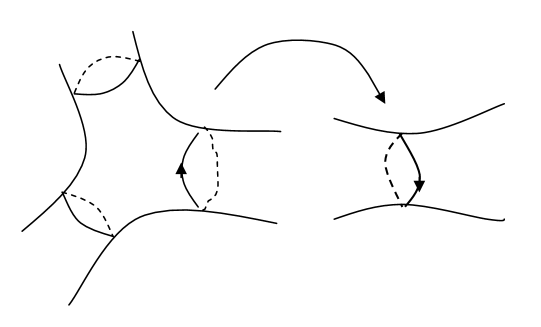
Figure 3. Orientation and labeling

Recall that for each curve $\gamma\in\Sigma$, there exist exactly two $\mathcal{S}$-pieces, say $S_{\gamma}^{+}$ and $S_{\gamma}^{-}$, such that $S_{\gamma}^{+}\cap S_{\gamma}^{-}=\gamma$. For each curve $\gamma\in\Sigma$, we can associate an orientation preserved by $f$. We may assume that the notations $S_{\gamma}^{+}$ and $S_{\gamma}^{-}$ are chosen such that $S_{\gamma}^{+}$ lies on the left side of $\gamma$ and $S_{\gamma}^{-}$ lies on the right side of $\gamma$.

Here, we borrow some notations from Lemma 3.1. Recall that $\Gamma_{0}$ is the collection of the $(f,P)$-periodic curves that generates $\Gamma$. For $n\geq 1$, the set $\Gamma_{n}$ is defined by $\Gamma_{n}=\{\gamma\in\Gamma;n\text{ is the first integer such that }f^{n}(\gamma)\in\Gamma_{0}\}$.

One may verify that if $\delta\in f^{-1}(\Gamma)$ is homotopic to a curve $\gamma\in\Gamma$ in $\mathbb{\overline{C}}-P$, then $\delta$ is necessarily contained in $S^{+}_{\gamma}\cup S^{-}_{\gamma}$. One may verify that if $\gamma\in\Gamma_{1}$, then $\delta\neq\gamma$; if $\gamma\in\Gamma_{k}$ for some $k\geq 2$, it can happen that $\delta=\gamma$.

For each curve $\gamma\in\Gamma=\bigcup_{n\geq 1}\Gamma_{n}$, we will associate two positive numbers $\rho(S_{\gamma}^{+},\gamma)$ and $\rho(S_{\gamma}^{-},\gamma)$ inductively, as follows:

If $\gamma\in\Gamma_{1}$, we choose two positive numbers $\rho(S_{\gamma}^{+},\gamma)$ and $\rho(S_{\gamma}^{-},\gamma)$ such that

$$\rho(S_{\gamma}^{+},\gamma)+\rho(S_{\gamma}^{-},\gamma)=1,$$

$$\sum_{\beta\in\Gamma}\sum_{\alpha\sim\gamma,\alpha\subset S_{\gamma}^{\omega}}\frac{v(\beta)}{{\rm deg}(f:\alpha\rightarrow\beta)}<v(\gamma)\rho(S_{\gamma}^{\omega},\gamma),\ \omega\in\{\pm\}.$$

Suppose that for each curve $\alpha\in\Gamma_{1}\cup\cdots\cup\Gamma_{k}$, we have already chosen two numbers $\rho(S_{\alpha}^{+},\alpha)$ and $\rho(S_{\alpha}^{-},\alpha)$. Then for $\gamma\in\Gamma_{k+1}$ (note that $f(\gamma)\in\Gamma_{k}$), we can find two positive numbers $\rho(S_{\gamma}^{+},\gamma)$ and $\rho(S_{\gamma}^{-},\gamma)$ such that:

$$\rho(S_{\gamma}^{+},\gamma)+\rho(S_{\gamma}^{-},\gamma)=1,$$

$$\frac{v(f(\gamma))}{{\rm deg}(f|_{\gamma})}\rho(S_{f(\gamma)}^{\omega},f(\gamma))+\sum_{\beta\in\Gamma}\sum_{\alpha\sim\gamma,\alpha\subset S_{\gamma}^{\omega}\setminus\gamma}\frac{v(\beta)}{{\rm deg}(f:\alpha\rightarrow\beta)}<v(\gamma)\rho(S_{\gamma}^{\omega},\gamma),\ \omega\in\{\pm\}.$$

In fact, we can take

$$\rho(S_{\gamma}^{\omega},\gamma)=\frac{\displaystyle\frac{v(f(\gamma))}{{\rm deg}(f|_{\gamma})}\rho(S_{f(\gamma)}^{\omega},f(\gamma))+\sum_{\beta\in\Gamma}\sum_{\alpha\sim\gamma,\alpha\subset S_{\gamma}^{\omega}\setminus\gamma}\frac{v(\beta)}{{\rm deg}(f:\alpha\rightarrow\beta)}}{\displaystyle\sum_{\beta\in\Gamma}\sum_{\alpha\sim\gamma}\frac{v(\beta)}{{\rm deg}(f:\alpha\rightarrow\beta)}},\ \omega\in\{\pm\}.$$

6.2. Equipotentials in the marked disks of rational maps

Suppose that $(f,P)$ is either a Thurston rational map or a Siegel rational map, with a non-empty Fatou set. Recall that $P$ is a marked set containing the postcritical set $P_{f}$. Then each periodic Fatou component is either a superattracting domain or a Siegel disk. If $f$ has a superattracting Fatou component $D$, then every Fatou component $\Delta$ which is eventually mapped onto $D$ can be marked by a unique pre-periodic point $a\in\Delta$. We call $(\Delta,a)$ a I-type marked disk of $f$. Note that every equipotential in a superattracting Fatou component corresponds to a round circle in Böttcher coordinate. If $f$ has a Siegel disk $D$, then it is known that the boundary $\partial D$ is contained in the postcritical set $P_{f}$. Let $z_{0}$ be the center of the Siegel disk $D$, the intersection $P\cap(D-\{z_{0}\})$ is either empty or consists of finitely many $(f,P)$-periodic analytic curves. Let $D_{0}\subset D$ be the component of $\mathbb{\overline{C}}-(P\setminus\{z_{0}\})$ containing $z_{0}$. For any $k\geq 0$ and any component $\Delta$ of $f^{-k}(D_{0})$, one can verify that $\Delta$ is a disk and there is a unique point $a\in\Delta\cap f^{-k}(z_{0})$. We call $(\Delta,a)$ a II-type marked disk of $(f,P)$.

In this way, for each Fatou component, we can associate a marked disk $(\Delta,a)$. An equipotential $\gamma$ of $(\Delta,a)$ is an analytic curve that is mapped to a round circle with center zero under a Riemann mapping $\phi:\Delta\rightarrow\mathbb{D}=\{|z|<1\}$ with $\phi(a)=0$. The potential $\varpi(\gamma)$ of $\gamma$ is defined to be $\textrm{mod}(A(\partial\Delta,\gamma))$, the modulus of the annulus between $\partial\Delta$ and $\gamma$. One may check that these definitions are independent of the choice of the map $\phi$.

6.3. A positive function

For each curve $\gamma\in\Sigma$, we associate an open annular neighborhood $A^{\gamma}$ of $\gamma$. The annulus $A^{\gamma}$ is chosen as follows: If $\gamma\in\Gamma_{0}$, we take $A^{\gamma}$ as a proper subset of the rotation annulus containing $\gamma$ such that $f(A^{\gamma})=A^{f(\gamma)}$ and $\overline{A^{\gamma}}\cap f(P-\cup\mathcal{A})=\emptyset$. If $\gamma\in\Gamma_{k}$ for some $k\geq 1$, then $A^{\gamma}$ is the component of $f^{-k}(A^{f^{k}(\gamma)})$ containing $\gamma$.

We define

$$\mathcal{S}^{\star}=\{U;\ U\text{ is a connected component of }\mathbb{\overline{C}}-\cup_{\gamma\in\Sigma}A^{\gamma}\},$$

$$\mathcal{E}^{\star}=\{{V};\ V\text{ is a connected component of }\mathbb{\overline{C}}-f^{-1}(\cup_{\gamma\in\Sigma}A^{\gamma})\}.$$

Each element of $\mathcal{S}^{\star}$ (resp. $\mathcal{E}^{\star}$) is called an $\mathcal{S}^{\star}$-piece (resp. $\mathcal{E}^{\star}$-piece). We will use $S^{\star}$ (resp. $E^{\star}$) to denote an $\mathcal{S}^{\star}$-piece (resp. $\mathcal{E}^{\star}$-piece). We remark that if we use $S$ to denote an $\mathcal{S}$-piece, then the notation $S^{*}$ means the unique $\mathcal{S}^{\star}$-piece contained in $S$; on the other hand, if we use $S^{*}$ to denote an $\mathcal{S}^{*}$-piece, then the notation $S$ means the unique $\mathcal{S}$-piece containing $S^{*}$. The convention also applies to the $\mathcal{E}$-pieces and $\mathcal{E}^{\star}$-pieces.

Similarly as in Section 3, we define $E_{S^{\star}}$ to be the unique $\mathcal{E}^{\star}$-piece parallel to $S^{\star}$. The map $f_{*}:\mathcal{S}^{\star}\rightarrow\mathcal{S}^{\star}$ is defined by $f_{*}(S^{\star})=f(E_{S^{\star}})$. The marked sphere $\mathbb{\overline{C}}(S^{\star})$, the marked disk extension $H_{S^{\star}}:\mathbb{\overline{C}}(S^{\star})\rightarrow\mathbb{\overline{C}}(f_{*}(S^{\star}))$, the marked set $P(S^{\star})$ and also the sets $\partial_{0}(S^{\star}),\partial_{1}(S^{\star}),\partial_{2}(S^{\star})$ are defined in the same way. Set

$$h^{\star}_{\nu}=H_{f_{*}^{p_{\nu}-1}(S^{\star}_{\nu})}\circ\cdots\circ H_{f_{*}(S^{\star}_{\nu})}\circ H_{S^{\star}_{\nu}},\ {P}^{\star}_{\nu}=P(S^{\star}_{\nu}),\ 1\leq\nu\leq n.$$

Consider the maps $(h_{\nu},P_{\nu})$ and $({h}^{\star}_{\nu},{P}^{\star}_{\nu})$ for $\ 1\leq\nu\leq n$. It is clear that

$\bullet$ $(h_{\nu},P_{\nu})$ has no Thurston obstructions iff $({h}^{\star}_{\nu},{P}^{\star}_{\nu})$ has no Thurston obstructions.

$\bullet$ $(h_{\nu},P_{\nu})$ is q.c-equivalent to a rational map iff $({h}^{\star}_{\nu},{P}^{\star}_{\nu})$ is q.c-equivalent to a rational map.

We will use $({h}^{\star}_{\nu},{P}^{\star}_{\nu})$ in place of $({h}_{\nu},{P}_{\nu})$ in the following discussions. This will allow us to construct deformations in a neighborhood of each curve $\gamma\in\Sigma$. The advantage of this replacement will be seen in the last step of the proof of Theorem 5.1 (see Section 6.6) where we apply the quasi-conformal surgery to glue all holomorphic models together to obtain a rational realization of $(f,P)$.

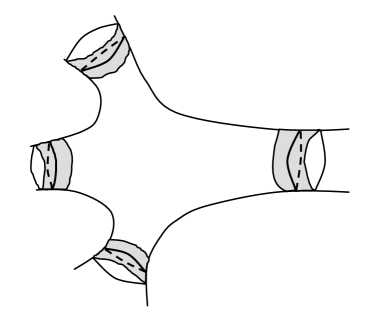
Figure 4. An $\mathcal{S}$-piece $S$ with boundary curves $\gamma_{1},\gamma_{2},\gamma_{3},\gamma_{4}$. $S$ contains an $\mathcal{S}^{\star}$-piece $S^{\star}$, whose boundary curves are $\beta_{1},\beta_{2},\beta_{3}$ and $\alpha_{4}$.

For each curve $\gamma\in\Sigma$, let $\alpha_{\gamma},\beta_{\gamma}$ be the two boundary curves of $A^{\gamma}$. Define

$$\Sigma^{\star}=\{\alpha_{\gamma},\beta_{\gamma};\gamma\in\Sigma\},\ \ \Gamma^{\star}=\{\alpha_{\gamma},\beta_{\gamma};\gamma\in\Gamma\},\ \ \Gamma_{k}^{\star}=\{\alpha_{\gamma},\beta_{\gamma};\gamma\in\Gamma_{k}\},k\geq 0.$$

We define a map $\pi:\Sigma^{\star}\rightarrow\Sigma$ by $\pi(\alpha)=\gamma$ if $\alpha$ is a boundary curve of $A^{\gamma}$. Obviously, for each curve $\gamma\in\Sigma$, we have $\pi^{-1}(\gamma)=\{\alpha_{\gamma},\beta_{\gamma}\}$. For $\delta\in\Sigma^{\star}$, let $S_{\delta}$ (resp. $S^{\star}_{\delta}$) be the unique $\mathcal{S}$-piece (resp. $\mathcal{S}^{\star}$-piece) containing $\delta$.

Now we define a positive function $\sigma_{t}:\Sigma^{\star}\rightarrow\mathbb{R}^{+}$, where $t$ is a positive parameter, as follows:

First, we consider $\gamma\in\Gamma_{0}^{\star}$. In this case, some iterate $f^{k}(\gamma)$ is contained in the rotation disk $\Delta$ of some Siegel map $(h^{\star}_{\nu},P^{\star}_{\nu})$. Note that there is a largest open annulus $A\subset\Delta$ such that

$\bullet$ the inner boundary of $A$ is $f^{k}(\gamma)$,

$\bullet$ $A\cap h^{\star}_{\nu}(P^{\star}_{\nu}-R_{D})=\emptyset$, where $R_{D}$ is the union of all rotation disks of $(h^{\star}_{\nu},P^{\star}_{\nu})$.

We define $\sigma_{t}(\gamma)$ to be the modulus of $A$. By definition, $\sigma_{t}(\gamma)=\sigma_{t}(f(\gamma)).$

Now, we consider $\gamma\in\Gamma^{\star}$. In this case, $\gamma\in\partial_{1}(S^{\star}_{\gamma})\cup\partial_{2}(S^{\star}_{\gamma})$. If $\gamma\in\partial_{1}(S^{\star}_{\gamma})$, we define

$$\sigma_{t}(\gamma)=t\cdot\rho(S_{\gamma},\pi(\gamma))\cdot v(\pi(\gamma)).$$

If $\gamma\in\partial_{2}(S^{\star}_{\gamma})$, we define

$$\sigma_{t}(\gamma)=\begin{cases}\dfrac{\sigma_{t}(f(\gamma))}{{\rm deg}(f|_{\gamma})},\ \ &\text{if }S^{\star}_{\gamma}\in\mathcal{S}^{\star}-\{S^{\star}_{1},\cdots,S^{\star}_{n}\},\\ t\cdot\rho(S_{\gamma},\pi(\gamma))\cdot v(\pi(\gamma)),\ \ &\text{if }S^{\star}_{\gamma}\in\{S^{\star}_{1},\cdots,S^{\star}_{n}\}.\end{cases}$$

In this way, for all curves $\gamma\in\Sigma^{\star}$, the quantity $\sigma_{t}(\gamma)$ is well-defined.

Lemma 6.2.

When $t$ is large enough, the function $\sigma_{t}:\Sigma^{\star}\rightarrow\mathbb{R}^{+}$ satisfies:

1. For any $\gamma\in\Gamma^{\star}$, $\sigma_{t}(\gamma)\leq t\cdot\rho(S_{\gamma},\pi(\gamma))\cdot v(\pi(\gamma))$.

2. For every $\gamma\in\Sigma$, suppose that $\pi^{-1}(\gamma)=\{\alpha_{\gamma},\beta_{\gamma}\}$. Then

$$\sigma_{t}(\alpha_{\gamma})+\sigma_{t}(\beta_{\gamma})\leq\begin{cases}tv(\gamma),\ \ &\text{if }\gamma\in\Gamma,\\ {\rm mod}(A_{\gamma}),\ \ &\text{if }\gamma\in\Gamma_{0},\end{cases}$$

where $A_{\gamma}$ is the rotation annulus of $(f,P)$ that contains $\gamma$ if $\gamma\in\Gamma_{0}$.

3. For every $\gamma\in\Gamma^{\star}$, if $\gamma\in\partial_{1}(S^{\star}_{\gamma})$, then we have the following inequality:

$$\sum_{\beta\in\Gamma^{\star}}\sum_{\alpha\sim\gamma,\alpha\subset S^{\star}_{\gamma}}\frac{\sigma_{t}(\beta)}{{\rm deg}(f:\alpha\rightarrow\beta)}<\sigma_{t}(\gamma),$$

where the second sum is taken over all components of $f^{-1}(\beta)$ contained in $S^{\star}_{\gamma}$ and homotopic to $\gamma$ in $\mathbb{\overline{C}}-P$ .

Proof.

1. Notice that if $\gamma\in\Gamma^{\star}$, then $\gamma\in\partial_{1}(S^{\star}_{\gamma})\cup\partial_{2}(S^{\star}_{\gamma})$. If $\gamma\in\partial_{1}(S^{\star}_{\gamma})$ or $S^{\star}_{\gamma}\in\{S^{\star}_{1},\cdots,S^{\star}_{n}\}$, then by evaluation, $\sigma_{t}(\gamma)=t\rho(S_{\gamma},\pi(\gamma))v(\pi(\gamma))$. Now suppose $\gamma\in\partial_{2}(S^{\star}_{\gamma})$ and $S^{\star}_{\gamma}\in\mathcal{S}^{\star}-\{S^{\star}_{1},\cdots,S^{\star}_{n}\}$. Let $p\geq 1$ be the first integer such that $f_{*}^{p}(S^{\star}_{\gamma})\in\{S^{\star}_{1},\cdots,S^{\star}_{n}\}$. There is a largest number $k\in\{0,\cdots,p\}$ such that $f^{j}(\gamma)\in\partial_{2}(f^{j}_{*}(S^{\star}_{\gamma}))$ for $0\leq j<k$. Thus we have

$$\sigma_{t}(\gamma)=\frac{\sigma_{t}(f(\gamma))}{{\rm deg}(f|_{\gamma})}=\cdots=\frac{\sigma_{t}(f^{k}(\gamma))}{{\rm deg}(f^{k}|_{\gamma})}.$$

If $f^{k}(\gamma)\in\partial_{0}(f^{k}_{*}(S^{\star}_{\gamma}))$, then $\sigma_{t}(f^{k}(\gamma))$ is a constant independent of $t$, thus $\sigma_{t}(\gamma)\leq t\rho(S_{\gamma},\pi(\gamma))v(\pi(\gamma))$ when $t$ is large.

If $f^{k}(\gamma)\in\partial_{1}(f^{k}_{*}(S^{\star}_{\gamma}))$, then

$$\sigma_{t}(\gamma)=\frac{t\cdot\rho(S_{f^{k}(\gamma)},\pi(f^{k}(\gamma)))\cdot v(\pi(f^{k}(\gamma)))}{{\rm deg}(f^{k}|_{\gamma})}.$$

By the choice of the numbers $\{\rho(S_{\gamma}^{+},\gamma),\rho(S_{\gamma}^{-},\gamma);\gamma\in\Gamma\}$, we see that for any curve $\beta\in\Gamma-\Gamma_{1}=\cup_{j\geq 2}\Gamma_{j}$,

$$\frac{v(f(\beta))\rho(S_{f(\beta)}^{\omega},f(\beta))}{{\rm deg}(f|_{\beta})}<v(\beta)\rho(S_{\beta}^{\omega},\beta),\ \omega\in\{\pm\}.$$

Since for each $\gamma\in\Gamma^{\star}$, ${\rm deg}(f|_{\gamma})={\rm deg}(f|_{\pi(\gamma)})$, we have that

$$\sigma_{t}(\gamma) < \frac{t\rho(S_{f^{k-1}(\gamma)},\pi(f^{k-1}(\gamma)))v(\pi(f^{k-1}(\gamma)))}{{\rm deg}(f^{k-1}|_{\gamma})}<\cdots$$

$$< \frac{t\rho(S_{f(\gamma)},\pi(f(\gamma)))v(\pi(f(\gamma)))}{{\rm deg}(f|_{\gamma})}<t\rho(S_{\gamma},\pi(\gamma))v(\pi(\gamma)).$$

If $f^{k}(\gamma)\in\partial_{2}(f^{k}_{*}(S^{\star}_{\gamma}))$, then we have $k=p$ by the choice of $k$ and

$$\sigma_{t}(\gamma)=\frac{t\rho(S_{f^{p}(\gamma)},\pi(f^{p}(\gamma)))v(\pi(f^{p}(\gamma)))}{{\rm deg}(f^{p}|_{\gamma})}.$$

With the same argument as above, we have $\sigma_{t}(\gamma)<t\rho(S_{\gamma},\pi(\gamma))v(\pi(\gamma))$.

2. The conclusion follows from 1 and the definition of $\sigma_{t}$.

3. We verify the inequality directly, as follows:

$$\sum_{\beta\in\Gamma^{\star}}\sum_{\alpha\sim\gamma,\alpha\subset S^{\star}_{\gamma}}\frac{\sigma_{t}(\beta)}{{\rm deg}(f:\alpha\rightarrow\beta)}$$

$$= \sum_{\beta\in\Gamma^{\star}}\sum_{\alpha\sim\gamma,\alpha\subset S^{\star}_{\gamma}\setminus{\gamma}}\frac{\sigma_{t}(\beta)}{{\rm deg}(f:\alpha\rightarrow\beta)}+\frac{\sigma_{t}(f(\gamma))}{{\rm deg}(f|_{\gamma})}$$

$$\leq \sum_{\beta\in\Gamma^{\star}}\sum_{\alpha\sim\gamma,\alpha\subset S^{\star}_{\gamma}\setminus{\gamma}}\frac{\sigma_{t}(\beta)}{{\rm deg}(f:\alpha\rightarrow\beta)}+\frac{t\rho(S_{f(\gamma)},\pi({f(\gamma)}))v(\pi({f(\gamma)}))}{{\rm deg}(f|_{\gamma})}\ \ (By\ 1)$$

$$= \sum_{\delta\in\Gamma}\sum_{\zeta\in\pi^{-1}(\delta)}\sum_{\alpha\sim\gamma,\alpha\subset S^{\star}_{\gamma}\setminus{\gamma}}\frac{\sigma_{t}(\zeta)}{{\rm deg}(f:\alpha\rightarrow\zeta)}+\frac{t\rho(S_{f(\gamma)},\pi({f(\gamma)}))v(\pi({f(\gamma)}))}{{\rm deg}(f|_{\gamma})}$$

$$= \sum_{\delta\in\Gamma}\sum_{\alpha\sim\pi(\gamma),\alpha\subset{S}_{\gamma}\setminus{\pi(\gamma)}}\frac{\sum_{\zeta\in\pi^{-1}(\delta)}\sigma_{t}(\zeta)}{{\rm deg}(f:\alpha\rightarrow\delta)}+\frac{t\rho(S_{f(\gamma)},\pi({f(\gamma)}))v(\pi({f(\gamma)}))}{{\rm deg}(f|_{\gamma})}$$

$$\leq \sum_{\delta\in\Gamma}\sum_{\alpha\sim\pi(\gamma),\alpha\subset{S}_{\gamma}\setminus{\pi(\gamma)}}\frac{tv(\delta)}{{\rm deg}(f:\alpha\rightarrow\delta)}+\frac{t\rho(S_{f(\gamma)},\pi({f(\gamma)}))v(\pi({f(\gamma)}))}{{\rm deg}(f|_{\gamma})}\ \ (By\ 2)$$

$$< t\rho(S_{\gamma},\pi(\gamma))v(\pi(\gamma))=\sigma_{t}(\gamma).\ \ (By\ the\ choice\ of\ the\ number\ \rho)$$

∎

6.4. Holomorphic models

We first decompose $\mathcal{S}^{\star}$ into $\mathcal{S}^{\star}_{0}\sqcup\mathcal{S}^{\star}_{1}\sqcup\cdots$, where

$$\mathcal{S}^{\star}_{0}=\{f_{*}^{j}(S^{\star}_{\nu});0\leq j<p_{\nu},1\leq\nu\leq n\},$$

$$\mathcal{S}^{\star}_{k}=\{S^{\star}\in\mathcal{S}^{\star};k\text{ is the first integer such that }f_{*}^{k}(S^{\star})\in\mathcal{S}^{\star}_{0}\},k\geq 1.$$

It’s obvious that $\mathcal{S}^{\star}_{0}$ consists of all $f_{*}$-periodic $\mathcal{S}^{\star}$-pieces.

Lemma 6.3 (Pre-holomorphic models).

Suppose $({h}_{\nu}^{\star},{P}^{\star}_{\nu})$ is q.c-equivalent to a rational map $(R_{\nu},Q_{\nu})$ via a pair of quasi-conformal maps $(\Phi_{\nu},\Psi_{\nu})$ for $1\leq\nu\leq n$. Then for each $\mathcal{S}^{\star}$-piece $S^{\star}$, there exist a pair of quasi-conformal maps $(\Phi_{S^{\star}},\Psi_{S^{\star}}):\mathbb{\overline{C}}(S^{\star})\rightarrow\mathbb{\overline{C}}$ and a rational map $R_{S^{\star}}$ such that $\Phi_{S^{\star}}$ is isotopic to $\Psi_{S^{\star}}$ rel $P(S^{\star})$ and the following diagram commutes:

Proof.

Using the same argument as the proof of the sufficiency of Theorem 5.1 (see Section 5.2, step 1), one can show that for any $1\leq\nu\leq n$ and any $0\leq k<p_{\nu}$, there exist a quasi-conformal map $\Phi_{f_{*}^{k}(S^{\star}_{\nu})}$ and a rational map $R_{f_{*}^{k}(S^{\star}_{\nu})}$ such that the following diagram commutes

We set $\Psi_{f_{*}^{k}(S^{\star}_{\nu})}=\Phi_{f_{*}^{k}(S^{\star}_{\nu})}$ for $0<k<p_{\nu}$.

For each $S^{\star}\in\mathcal{S}^{\star}_{1}$, notice that $f_{*}(S^{\star})\in\mathcal{S}^{\star}_{0}$, we pull back the standard complex structure of $\mathbb{\overline{C}}$ to $\mathbb{\overline{C}}(S^{\star})$ via $\Phi_{f_{*}(S^{\star})}\circ H_{S^{\star}}$ and integrate it to get a quasi-conformal map $\Phi_{S^{\star}}:\mathbb{\overline{C}}(S^{\star})\rightarrow\mathbb{\overline{C}}$. Then $R_{S^{\star}}:=\Phi_{f_{*}(S^{\star})}\circ H_{S^{\star}}\circ\Phi_{S^{\star}}^{-1}$ is a rational map. We set $\Psi_{S^{\star}}=\Phi_{S^{\star}}$.

By the inductive procedure, for each $\mathcal{S}^{\star}_{k}$-piece ($k=2,3,\cdots$), we can get a pair of quasi-conformal maps $(\Phi_{S^{\star}},\Psi_{S^{\star}})$ and a rational map $R_{S^{\star}}$, as required. ∎

Lemma 6.4 (Holomorphic models for periodic pieces).

Fix a periodic piece $S^{\star}\in\mathcal{S}^{\star}_{0}$. Let $p$ be the period of $S^{\star}$. Then for any large parameter $t>0$, there exist a pair of quasi-conformal maps $(\Phi^{t}_{S^{\star}},\Psi^{t}_{S^{\star}}):\mathbb{\overline{C}}(S^{\star})\rightarrow\mathbb{\overline{C}}$ such that

1. $\Psi^{t}_{S^{\star}}$ is isotopic to $\Phi^{t}_{S^{\star}}$ rel $P(S^{\star})$.

2. $\Phi^{t}_{f_{*}(S^{\star})}\circ f\circ(\Psi^{t}_{S^{\star}})^{-1}|_{\Psi^{t}_{S^{\star}}(E_{S^{\star}})}=R_{S^{\star}}|_{\Psi^{t}_{S^{\star}}(E_{S^{\star}})}$, where $R_{S^{\star}}$ is defined in Lemma 6.3.

3. The return map $f_{i}:=R_{f_{*}^{i-1}(S^{\star})}\circ\cdots\circ R_{S^{\star}}\circ R_{f_{*}^{p-1}(S^{\star})}\circ\cdots\circ R_{f_{*}^{i}(S^{\star})}$ is either a Siegel map or a Thurston map.

4. For each $i\geq 0$ and each curve $\gamma\in\partial(f^{i}_{*}(S^{\star}))$, let $\beta_{\gamma}$ be the boundary curve of $E_{f^{i}_{*}(S^{\star})}$ such that either $\gamma=\beta_{\gamma}$, or $\gamma$ and $\beta_{\gamma}$ bound an annulus in $S^{\star}-P$. Then both $\Phi^{t}_{f_{*}^{i}(S^{\star})}(\gamma)$ and $\Psi^{t}_{f_{*}^{i}(S^{\star})}(\beta_{\gamma})$ are equipotentials in the same marked disk of $f_{i}$, with potentials

$$\varpi(\Phi^{t}_{f_{*}^{i}(S^{\star})}(\gamma))=\sigma_{t}(\gamma),\ \varpi(\Psi^{t}_{f_{*}^{i}(S^{\star})}(\beta_{\gamma}))=\frac{\sigma_{t}(f(\beta_{\gamma}))}{{\deg(f|_{\beta_{\gamma}})}}.$$

Proof.

For each $\nu\in[1,n]$ and each $i\geq 0$, the critical values of $H_{f_{*}^{i}(S^{\star}_{\nu})}$ are contained in $P(f_{*}^{i+1}(S^{\star}_{\nu}))$ and $H_{f_{*}^{i}(S^{\star}_{\nu})}(P(f_{*}^{i}(S^{\star}_{\nu})))\subset P(f_{*}^{i+1}(S^{\star}_{\nu}))$. Let $(\Phi_{f_{*}^{i}(S^{\star}_{\nu})},\Psi_{f_{*}^{i}(S^{\star}_{\nu})}):\mathbb{\overline{C}}(f_{*}^{i}(S^{\star}_{\nu}))\rightarrow\mathbb{\overline{C}}$ be the quasi-conformal maps constructed in Lemma 6.3. Since $\Phi_{S^{\star}_{\nu}}$ is isotopic to $\Psi_{S^{\star}_{\nu}}$ rel ${P}^{\star}_{\nu}=P(S^{\star}_{\nu})$, there is a quasi-conformal map $\phi_{f_{*}^{p_{\nu}-1}(S^{\star}_{\nu})}:\mathbb{\overline{C}}(f_{*}^{p_{\nu}-1}(S^{\star}_{\nu}))\rightarrow\mathbb{\overline{C}}$ isotopic to $\Phi_{f_{*}^{p_{\nu}-1}(S^{\star}_{\nu})}$ rel $P(f_{*}^{p_{\nu}-1}(S^{\star}_{\nu}))$ and $\Psi_{S^{\star}_{\nu}}\circ H_{f_{*}^{p_{\nu}-1}(S^{\star}_{\nu})}=R_{f_{*}^{p_{\nu}-1}(S^{\star}_{\nu})}\circ\phi_{f_{*}^{p_{\nu}-1}(S^{\star}_{\nu})}$. Inductively, there is a sequence of quasi-conformal maps $\phi_{f_{*}^{i}(S^{\star}_{\nu})}:\mathbb{\overline{C}}(f_{*}^{i}(S^{\star}_{\nu}))\rightarrow\mathbb{\overline{C}}$ for $i=p_{\nu}-2,\cdots,1$, such that $\phi_{f_{*}^{i}(S^{\star}_{\nu})}$ is isotopic to $\Phi_{f_{*}^{i}(S^{\star}_{\nu})}$ rel $P(f_{*}^{i}(S^{\star}_{\nu}))$ and the following diagram commutes:

This diagram together with the diagram in Lemma 6.3 implies that for any $1\leq i<p_{\nu}$, the map $H_{f_{*}^{i-1}(S^{\star}_{\nu})}\circ\cdots\circ H_{S^{\star}_{\nu}}\circ H_{f_{*}^{p_{\nu}-1}(S^{\star}_{\nu})}\circ\cdots\circ H_{f_{*}^{i}(S^{\star}_{\nu})}$ is q.c-equivalent to $f_{i}=R_{f_{*}^{i-1}(S^{\star}_{\nu})}\circ\cdots\circ R_{S^{\star}_{\nu}}\circ R_{f_{*}^{p_{\nu}-1}(S^{\star}_{\nu})}\circ\cdots\circ R_{f_{*}^{i}(S^{\star}_{\nu})}$ via $(\Phi_{f_{*}^{i}(S^{\star}_{\nu})},\phi_{f_{*}^{i}(S^{\star}_{\nu})})$. Notice that $f_{i}(\phi_{f_{*}^{i}(S^{\star}_{\nu})}(P(f_{*}^{i}(S^{\star}_{\nu}))))\subset\phi_{f_{*}^{i}(S^{\star}_{\nu})}(P(f_{*}^{i}(S^{\star}_{\nu})))$, $f_{i}$ is either a Siegel map or a Thurston map.

The relation $f_{i+1}\circ R_{f_{*}^{i}(S^{\star}_{\nu})}=R_{f_{*}^{i}(S^{\star}_{\nu})}\circ f_{i}$ with $f_{p_{\nu}}=R_{\nu}$ (here, $R_{\nu}$ is the rational map defined in Lemma 6.3) means that $R_{f_{*}^{i}(S^{\star}_{\nu})}$ is a semi-conjugacy between $f_{i+1}$ and $f_{i}$, so their Julia sets satisfy $J(f_{i})=R_{f_{*}^{i}(S^{\star}_{\nu})}^{-1}(J(f_{i+1}))$. One can check that $R_{f_{*}^{i}(S^{\star}_{\nu})}$ maps the marked disks of $f_{i}$ onto the marked disks of $f_{i+1}$, and maps the equipotentials of $f_{i}$ to the equipotentials of $f_{i+1}$.

In the following, we will construct a pair of quasi-conformal maps $(\Phi^{t}_{S^{\star}},\Psi^{t}_{S^{\star}}):\mathbb{\overline{C}}(S^{\star})\rightarrow\mathbb{\overline{C}}$ that satisfy the required properties.

Step 1: Construction of $\Phi^{t}_{S^{\star}_{\nu}}$ and ${\Phi}^{t}_{f_{*}^{p_{\nu}-1}(S^{\star}_{\nu})}$. We first modify $\Phi_{S^{\star}_{\nu}}$ to a new quasi-conformal map $\Phi^{t}_{S^{\star}_{\nu}}:\mathbb{\overline{C}}(S^{\star}_{\nu})\rightarrow\mathbb{\overline{C}}$ such that $\Phi^{t}_{S^{\star}_{\nu}}$ is isotopic to $\Phi_{S^{\star}_{\nu}}$ rel $P(S^{\star}_{\nu})$, and for each curve $\gamma\in\partial(S^{\star}_{\nu})$, the curve $\Phi^{t}_{S^{\star}_{\nu}}(\gamma)$ is the equipotential in a marked disk of $f_{p_{\nu}}=R_{\nu}$ with potential $\varpi(\Phi^{t}_{S^{\star}_{\nu}}(\gamma))=\sigma_{t}(\gamma)$. Then, we lift $\Phi^{t}_{S^{\star}_{\nu}}$ via $R_{f_{*}^{p_{\nu}-1}(S^{\star}_{\nu})}$ and $H_{f_{*}^{p_{\nu}-1}(S^{\star}_{\nu})}$ and get a quasi-conformal map $\widehat{\Phi}^{t}_{f_{*}^{p_{\nu}-1}(S^{\star}_{\nu})}$ isotopic to $\Phi_{f_{*}^{p_{\nu}-1}(S^{\star}_{\nu})}$ rel $P(f_{*}^{p_{\nu}-1}(S^{\star}_{\nu}))$. See the following commutative diagram:

Now, we modify $H_{f_{*}^{p_{\nu}-1}(S^{\star}_{\nu})}$ to another marked disk extension of $f|_{E_{f_{*}^{p_{\nu}-1}(S^{\star}_{\nu})}}$, say $\widehat{H}_{f_{*}^{p_{\nu}-1}(S^{\star}_{\nu})}$, such that for each curve $\gamma\in\partial_{1}(f_{*}^{p_{\nu}-1}(S^{\star}_{\nu}))$, the curve $\Phi^{t}_{S^{\star}_{\nu}}(\widehat{H}_{f_{*}^{p_{\nu}-1}(S^{\star}_{\nu})}(\gamma))$ is an equipotential in some marked disk of $f_{p_{\nu}}=R_{\nu}$. Since $\gamma\in\partial_{1}(f_{*}^{p_{\nu}-1}(S^{\star}_{\nu}))$, the potential of $\Phi^{t}_{S^{\star}_{\nu}}(\widehat{H}_{f_{*}^{p_{\nu}-1}(S^{\star}_{\nu})}(\gamma))$ should be larger than $\varpi(\Phi^{t}_{S^{\star}_{\nu}}(f(\beta_{\gamma})))=\sigma_{t}(f(\beta_{\gamma}))$. It follows from Lemma 6.2 that $\deg(f|_{\beta_{\gamma}})\sigma_{t}(\gamma)>\sigma_{t}(f(\beta_{\gamma}))$ when $t$ is large. So it is reasonable to designate $\varpi(\Phi^{t}_{S^{\star}_{\nu}}(\widehat{H}_{f_{*}^{p_{\nu}-1}(S^{\star}_{\nu})}(\gamma)))$ to be $\deg(f|_{\beta_{\gamma}})\cdot\sigma_{t}(\gamma)$.

Since both $H_{f_{*}^{p_{\nu}-1}(S^{\star}_{\nu})}$ and $\widehat{H}_{f_{*}^{p_{\nu}-1}(S^{\star}_{\nu})}$ are marked disk extensions of $f|_{E_{f_{*}^{p_{\nu}-1}(S^{\star}_{\nu})}}$, there is a quasi-conformal map $\xi_{p_{\nu}-1}:\mathbb{\overline{C}}(f_{*}^{p_{\nu}-1}(S^{\star}_{\nu}))\rightarrow\mathbb{\overline{C}}(f_{*}^{p_{\nu}-1}(S^{\star}_{\nu}))$ isotopic to the identity map rel $E_{f_{*}^{p_{\nu}-1}(S^{\star}_{\nu})}\cup P(f_{*}^{p_{\nu}-1}(S^{\star}_{\nu}))$ such that $\widehat{H}_{f_{*}^{p_{\nu}-1}(S^{\star}_{\nu})}=H_{f_{*}^{p_{\nu}-1}(S^{\star}_{\nu})}\circ\xi_{p_{\nu}-1}$.

We set ${\Phi}^{t}_{f_{*}^{p_{\nu}-1}(S^{\star}_{\nu})}=\widehat{\Phi}^{t}_{f_{*}^{p_{\nu}-1}(S^{\star}_{\nu})}\circ\xi_{p_{\nu}-1}$. It’s obvious that $\Phi^{t}_{S^{\star}_{\nu}}\circ\widehat{H}_{f_{*}^{p_{\nu}-1}(S^{\star}_{\nu})}=R_{f_{*}^{p_{\nu}-1}(S^{\star}_{\nu})}\circ{\Phi}^{t}_{f_{*}^{p_{\nu}-1}(S^{\star}_{\nu})}$.

Step 2: Construction of $\Phi^{t}_{f^{i}_{*}(S^{\star}_{\nu})}$ for $i=p_{\nu}-2,\cdots,1$ and ${\Psi}^{t}_{S^{\star}_{\nu}}$. By the same argument as in Step 1, we can lift ${\Phi}^{t}_{f_{*}^{p_{\nu}-1}(S^{\star}_{\nu})}$ via $R_{f_{*}^{p_{\nu}-2}(S^{\star}_{\nu})}$ and $H_{f_{*}^{p_{\nu}-2}(S^{\star}_{\nu})}$ and get a map $\widehat{\Phi}^{t}_{f_{*}^{p_{\nu}-2}(S^{\star}_{\nu})}$ isotopic to $\Phi_{f_{*}^{p_{\nu}-2}(S^{\star}_{\nu})}$ rel $P(f_{*}^{p_{\nu}-2}(S^{\star}_{\nu}))$. Then we modify $H_{f_{*}^{p_{\nu}-2}(S^{\star}_{\nu})}$ to another marked disk extension of $f|_{E_{f_{*}^{p_{\nu}-2}(S^{\star}_{\nu})}}$, say $\widehat{H}_{f_{*}^{p_{\nu}-2}(S^{\star}_{\nu})}=H_{f_{*}^{p_{\nu}-2}(S^{\star}_{\nu})}\circ\xi_{p_{\nu}-2}$, where $\xi_{p_{\nu}-2}:\mathbb{\overline{C}}(f_{*}^{p_{\nu}-2}(S^{\star}_{\nu}))\rightarrow\mathbb{\overline{C}}(f_{*}^{p_{\nu}-2}(S^{\star}_{\nu}))$ is a quasi-conformal map isotopic to the identity map rel $E_{f_{*}^{p_{\nu}-2}(S^{\star}_{\nu})}\cup P(f_{*}^{p_{\nu}-2}(S^{\star}_{\nu}))$, such that for each $\gamma\in\partial_{1}(f_{*}^{p_{\nu}-2}(S^{\star}_{\nu}))$, the curve $\Phi^{t}_{f_{*}^{p_{\nu}-1}(S^{\star}_{\nu})}(\widehat{H}_{f_{*}^{p_{\nu}-2}(S^{\star}_{\nu})}(\gamma))$ is an equipotential of $f_{p_{\nu}-1}$ with potential equal to $\deg(f|_{\beta_{\gamma}})\sigma_{t}(\gamma)$. We set ${\Phi}^{t}_{f_{*}^{p_{\nu}-2}(S^{\star}_{\nu})}=\widehat{\Phi}^{t}_{f_{*}^{p_{\nu}-2}(S^{\star}_{\nu})}\circ\xi_{p_{\nu}-2}$.

Inductively, we can get a sequence of new marked disk extensions $\widehat{H}_{f_{*}^{i}(S^{\star}_{\nu})},i=p_{\nu}-1,\cdots,0,$ and a sequence of quasi-conformal maps $\Phi^{t}_{f_{*}^{i}(S^{\star}_{\nu})},i=p_{\nu}-1,\cdots,1,\ \Psi^{t}_{S^{\star}_{\nu}}$ such that the following diagram commutes

Moreover, for each $i\in[0,p_{\nu}-1]$ and each curve $\gamma\in\partial_{1}(f_{*}^{i}(S^{\star}_{\nu}))$, we require

$$\varpi(\Phi^{t}_{f_{*}^{i+1}(S^{\star}_{\nu})}(\widehat{H}_{f_{*}^{i}(S^{\star}_{\nu})}(\gamma)))=\deg(f|_{\beta_{\gamma}})\sigma_{t}(\gamma).$$

Finally, we set $\Psi^{t}_{f_{*}^{i}(S^{\star}_{\nu})}=\Phi^{t}_{f_{*}^{i}(S^{\star}_{\nu})}$ for $1\leq i\leq p_{\nu}-1$.

Step 3: Prescribed potentials. In this step, we will show that for each $0\leq i\leq p_{\nu}-1$ and each curve $\gamma\in\partial(f_{*}^{i}(S^{\star}_{\nu}))$,

(2) $$\varpi(\Phi^{t}_{f_{*}^{i}(S^{\star}_{\nu})}(\gamma))=\sigma_{t}(\gamma),\ \varpi(\Psi^{t}_{f_{*}^{i}(S^{\star}_{\nu})}(\beta_{\gamma}))=\frac{\sigma_{t}(f(\beta_{\gamma}))}{{\deg(f|_{\beta_{\gamma}})}}.$$

Notice that for each curve $\gamma\in\partial(S^{\star}_{\nu})\cup\cup_{0<i<p_{\nu}}\partial_{0}(f_{*}^{i}(S^{\star}_{\nu}))$, the first equation of (2) holds by the evaluation of $\varpi$.

If $\gamma\in\partial_{1}(f_{*}^{i}(S^{\star}_{\nu}))$ for some $0<i<p_{\nu}$, then by Step 2, $\Phi^{t}_{f_{*}^{i+1}(S^{\star}_{\nu})}(\widehat{H}_{f_{*}^{i}(S^{\star}_{\nu})}(\gamma))$ is an equipotential in a marked disk $(\Delta_{i+1},a)$ of $f_{i+1}$. Since $\Phi^{t}_{f_{*}^{i+1}(S^{\star}_{\nu})}\circ\widehat{H}_{f_{*}^{i}(S^{\star}_{\nu})}(\gamma)=R_{f_{*}^{i}(S^{\star}_{\nu})}\circ{\Phi}^{t}_{f_{*}^{i}(S^{\star}_{\nu})}(\gamma)$, we conclude that $\Phi^{t}_{f_{*}^{i}(S^{\star}_{\nu})}(\gamma)$ is also an equipotential of some marked disk of $f_{i}$, denoted by $(\Delta_{i},b)$. Then $R_{f_{*}^{i}(S^{\star}_{\nu})}:\Delta_{i}-\{b\}\rightarrow\Delta_{i+1}-\{a\}$ is a covering map of degree ${\deg}(f|_{\beta_{\gamma}})$. The potential of ${\Phi}^{t}_{f_{*}^{i}(S^{\star}_{\nu})}(\gamma)$ satisfies (here, we use $A(\alpha,\beta)$ to denote the annulus bounded by $\alpha$ and $\beta$)

$$\varpi({\Phi}^{t}_{f_{*}^{i}(S^{\star}_{\nu})}(\gamma)) = {\rm mod}\Big{(}A(\partial\Delta_{i},{\Phi}^{t}_{f_{*}^{i}(S^{\star}_{\nu})}(\gamma))\Big{)}$$

$$= {\rm mod}\Big{(}A(\partial\Delta_{i+1},{\Phi}^{t}_{f_{*}^{i+1}(S^{\star}_{\nu})}(\widehat{H}_{f_{*}^{i}(S^{\star}_{\nu})}(\gamma)))\Big{)}/{\deg}(f|_{\beta_{\gamma}})$$

$$= \varpi(\Phi^{t}_{f_{*}^{i+1}(S^{\star}_{\nu})}(\widehat{H}_{f_{*}^{i}(S^{\star}_{\nu})}(\gamma)))/{\deg}(f|_{\beta_{\gamma}})$$

$$= \sigma_{t}(\gamma).$$

Now we consider $\gamma\in\partial_{2}(f_{*}^{i}(S^{\star}_{\nu}))$ for some $0<i<p_{\nu}$. In this case, by the same argument as above, we can see that

$$\varpi(\Phi^{t}_{f_{*}^{i}(S^{\star}_{\nu})}(\gamma))=\frac{\varpi(\Phi^{t}_{f_{*}^{i+1}(S^{\star}_{\nu})}(f(\gamma)))}{{\deg}(f|_{\gamma})}.$$

By the definition of $\sigma_{t}$, for $\gamma\in\partial_{2}(f_{*}^{i}(S^{\star}_{\nu}))$, we have

$$\sigma_{t}(\gamma)=\frac{\sigma_{t}(f(\gamma))}{{\deg}(f|_{\gamma})}.$$

Based on this observation, we conclude by induction that $\varpi({\Phi}^{t}_{f_{*}^{i}(S^{\star}_{\nu})}(\gamma))=\sigma_{t}(\gamma)$.

Finally, we show that the second equation of (2) holds. Since for each $i\in[0,p_{\nu}-1]$ and each curve $\gamma\in\partial(f_{*}^{i}(S^{\star}_{\nu}))$, the curve $\Phi^{t}_{f_{*}^{i+1}(S^{\star}_{\nu})}(f(\beta_{\gamma}))$ is an equipotential, it follows from the relation

$$\Phi^{t}_{f^{i+1}_{*}(S^{\star}_{\nu})}\circ f\circ(\Psi^{t}_{f^{i}_{*}(S^{\star}_{\nu})})^{-1}|_{\Psi^{t}_{f^{i}_{*}(S^{\star}_{\nu})}(E_{f^{i}_{*}(S^{\star}_{\nu})})}=R_{f^{i}_{*}(S^{\star}_{\nu})}|_{\Psi^{t}_{f^{i}_{*}(S^{\star}_{\nu})}(E_{f^{i}_{*}(S^{\star}_{\nu})})}$$

that $\Psi^{t}_{f_{*}^{i}(S^{\star}_{\nu})}(\beta_{\gamma})$ is also an equipotential. The same argument as above yields

$$\varpi(\Psi^{t}_{f_{*}^{i}(S^{\star}_{\nu})}(\beta_{\gamma}))=\frac{\varpi(\Phi^{t}_{f_{*}^{i+1}(S^{\star}_{\nu})}(f(\beta_{\gamma})))}{{\deg}(f|_{\beta_{\gamma}})}=\frac{\sigma_{t}(f(\beta_{\gamma}))}{{\deg}(f|_{\beta_{\gamma}})}.$$

The proof is completed. ∎

Now, we deal with the strictly pre-periodic $\mathcal{S}^{\star}$-pieces. Let $S^{\star}\in\mathcal{S}^{\star}_{k}$ for some $k\geq 1$. Then $f_{*}^{k}(S^{\star})$ is a $f_{*}$-periodic $\mathcal{S}^{\star}$-piece. Notice that for $0\leq i<k$, $H_{f_{*}^{i}(S^{\star})}(P(f_{*}^{i}(S^{\star})))\subset P(f_{*}^{i+1}(S^{\star}))$ and each critical value of $H_{f_{*}^{i}(S^{\star})}$ is contained in $P(f_{*}^{i+1}(S^{\star}))$, we have that $R_{f_{*}^{i}(S^{\star})}\circ\Phi_{f_{*}^{i}(S^{\star})}(P(f_{*}^{i}(S^{\star})))\subset\Phi_{f_{*}^{i+1}(S^{\star})}(P(f_{*}^{i+1}(S^{\star})))$ and every critical value of $R_{f_{*}^{k-1}(S^{\star})}\circ\cdots\circ R_{S^{\star}}$ is contained in $\Phi_{f_{*}^{k}(S^{\star})}(P(f_{*}^{k}(S^{\star})))=\Phi^{t}_{f_{*}^{k}(S^{\star})}(P(f_{*}^{k}(S^{\star})))$, here $R_{f_{*}^{i}(S^{\star})}$ and $\Phi_{f_{*}^{i}(S^{\star})}$ are defined in Lemma 6.3. For any marked point $a\in P(S^{\star})\cap(\mathbb{\overline{C}}(S^{\star})-S^{\star})$, the point $R_{f_{*}^{k-1}(S^{\star})}\circ\cdots\circ R_{S^{\star}}(\Phi_{S^{\star}}(a))$ is the center of some marked disk $(\Delta,q)$ of some $f_{j}$, where $f_{j}$ is a return map defined in Lemma 6.4. The component $\Delta_{\Phi_{S^{\star}}(a)}$ of $(R_{f_{*}^{k-1}(S^{\star})}\circ\cdots\circ R_{S^{\star}})^{-1}(\Delta)$ that contains $\Phi_{S^{\star}}(a)$ is also a disk. We call $(\Delta_{\Phi_{S^{\star}}(a)},\Phi_{S^{\star}}(a))$ a marked disk of $R_{f_{*}^{k-1}(S^{\star})}\circ\cdots\circ R_{S^{\star}}$.

With the same argument as that of Lemma 6.4, we can show that

Lemma 6.5.

For any $k\geq 1$, any $S^{\star}\in\mathcal{S}^{\star}_{k}$ and any large parameter $t>0$, there exist a pair of quasi-conformal maps $\Phi^{t}_{S^{\star}}=\Psi^{t}_{S^{\star}}:\mathbb{\overline{C}}(S^{\star})\rightarrow\mathbb{\overline{C}}$ such that

1. $\Phi^{t}_{f_{*}(S^{\star})}\circ f\circ(\Psi^{t}_{S^{\star}})^{-1}|_{\Psi^{t}_{S^{\star}}(E_{S^{\star}})}=R_{S^{\star}}|_{\Psi^{t}_{S^{\star}}(E_{S^{\star}})}$, where $R_{S^{\star}}$ is defined in Lemma 6.3.

2. For each curve $\gamma\in\partial(S^{\star})$, let $\beta_{\gamma}$ be the unique curve in $\partial(E_{S^{\star}})$ homotopic to $\gamma$ in $\mathbb{\overline{C}}-P$. Then both $\Phi^{t}_{S^{\star}}(\gamma)$ and $\Phi^{t}_{S^{\star}}(\beta_{\gamma})$ are equipotentials in the same marked disk of $R_{f_{*}^{k-1}(S^{\star})}\circ\cdots\circ R_{S^{\star}}$, with potentials

$$\varpi(\Phi^{t}_{S^{\star}}(\gamma))=\sigma_{t}(\gamma),\ \varpi(\Phi^{t}_{S^{\star}}(\beta_{\gamma}))=\frac{\sigma_{t}(f(\beta_{\gamma}))}{{\deg(f|_{\beta_{\gamma}})}}.$$

We decompose $\mathcal{E}^{\star}$ into $\mathcal{E}^{\star}_{ess}\sqcup\mathcal{E}^{\star}_{A}\sqcup\mathcal{E}^{\star}_{D}$, where

$\bullet$ $\mathcal{E}^{\star}_{ess}=\{E_{S^{\star}};S^{\star}\in\mathcal{S}^{\star}\}$, it consists of all $\mathcal{E}^{\star}$-pieces parallel to some $\mathcal{S}^{\star}$-piece;

$\bullet$ $\mathcal{E}^{\star}_{A}$ is the collection of all $\mathcal{E}^{\star}$-pieces $E^{\star}$ contained essentially in an annular component of $S^{\star}-E_{S^{\star}}$ for some $\mathcal{S}^{\star}$-piece $S^{\star}$ (here, ‘essential’ means at least one boundary curve of $E^{\star}$ is non-peripheral in $\mathbb{\overline{C}}-P$);

$\bullet$ $\mathcal{E}^{\star}_{D}=\mathcal{E}^{\star}-(\mathcal{E}^{\star}_{ess}\sqcup\mathcal{E}^{\star}_{A})$. One may verify that each $\mathcal{E}^{\star}_{D}$-piece is contained in a disk component of $S^{\star}-E_{S^{\star}}\cup(\cup\mathcal{E}^{\star}_{ess})$ for some $\mathcal{S}^{\star}$-piece $S^{\star}$.

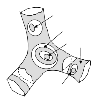
Figure 5. Different types of $\mathcal{E}^{\star}$-pieces: Here, $S^{\star}$ is an $\mathcal{S}^{\star}$-piece with boundary $\partial S^{\star}=\gamma_{1}\cup\gamma_{2}\cup\gamma_{3}$. $E^{\star}_{0}$ is an $\mathcal{E}^{\star}_{ess}$-piece. $E^{\star}_{5}$ and $E^{\star}_{6}$ are $\mathcal{E}^{\star}_{A}$-pieces. $E^{\star}_{1},E^{\star}_{2}$, $E^{\star}_{3}$ and $E^{\star}_{4}$ are $\mathcal{E}^{\star}_{D}$-pieces.

In the following, for every $\mathcal{E}^{\star}_{A}$-piece $E^{\star}$, we will construct a holomorphic model for $f|_{E^{\star}}$. Given an $\mathcal{E}^{\star}_{A}$-piece $E^{\star}$, first notice that $E^{\star}$ has no intersection with the marked set $P$. As we did before, we also associate a Riemann sphere $\mathbb{\overline{C}}(E^{\star})$ for $E^{\star}$. We mark a point in each component of $\mathbb{\overline{C}}(E^{\star})-E^{\star}$, and let $P(E^{\star})$ be the collection of all these marked points. We can get a marked disk extension of $f|_{E^{\star}}$, say $H_{E^{\star}}:\mathbb{\overline{C}}(E^{\star})\rightarrow\mathbb{\overline{C}}(f(E^{\star}))$, such that $H_{E^{\star}}|_{E^{\star}}=f|_{E^{\star}}$, $H_{E^{\star}}(P(E^{\star}))\subset P(f(E^{\star}))$ and all critical values (if any) of $H_{E^{\star}}$ are contained in $P(f(E^{\star}))$. Let $\Phi^{t}_{E^{\star}}:\mathbb{\overline{C}}(E^{\star})\rightarrow\mathbb{\overline{C}}$ be a quasi-conformal map such that $R_{E^{\star}}:=\Phi^{t}_{f(E^{\star})}\circ H_{E^{\star}}\circ(\Phi^{t}_{E^{\star}})^{-1}$ is holomorphic. We give a remark that if we change $\Phi^{t}_{f(E^{\star})}$ to another quasi-conformal map $\Phi^{t_{1}}_{f(E^{\star})}$ isotopic to $\Phi^{t}_{f(E^{\star})}$ rel $P(f(E^{\star}))$, then we can modify $\Phi^{t}_{E^{\star}}$ to a new map $\Phi^{t_{1}}_{E^{\star}}$, isotopic to $\Phi^{t}_{E^{\star}}$ rel $P(E^{\star})$, such that $R_{E^{\star}}=\Phi^{t_{1}}_{f(E^{\star})}\circ H_{E^{\star}}\circ(\Phi^{t_{1}}_{E^{\star}})^{-1}$. This means that once we get the holomorphic map $R_{E^{\star}}$, we can always assume that it is independent of the parameter $t$. We set $\Psi^{t}_{E^{\star}}=\Phi^{t}_{E^{\star}}$.

The $\mathcal{E}^{\star}_{A}$-piece $E^{\star}$ has exactly two boundary curves $\alpha$ and $\beta$ which are non-peripheral and homotopic to each other in $\mathbb{\overline{C}}-P$. By the choice of $\Phi^{t}_{S^{\star}}$ for $S^{\star}\in\mathcal{S}^{\star}$, both $\Phi^{t}_{f(E^{\star})}(f(\alpha))$ and $\Phi^{t}_{f(E^{\star})}(f(\beta))$ are equipotentials in the marked disks of some $f_{j}$ (defined in Lemma 6.4) or some $R_{f_{*}^{k-1}(S^{\star})}\circ\cdots\circ R_{S^{\star}}$. We denote the marked disk that contains $\Phi^{t}_{f(E^{\star})}(f(\alpha))$ (resp. $\Phi^{t}_{f(E^{\star})}(f(\beta))$) by $(\Delta_{a},a)$ (resp. $(\Delta_{b},b)$). It can happen that $(\Delta_{a},a)=(\Delta_{b},b)$. Let $\Delta_{\alpha}$ (resp. $\Delta_{\beta}$) be the component of $R_{E^{\star}}^{-1}(\Delta_{a})$ (resp. $R_{E^{\star}}^{-1}(\Delta_{b})$) that contains $\Phi^{t}_{E^{\star}}(\alpha)$ (resp. $\Phi^{t}_{E^{\star}}(\beta)$). Then $\Delta_{\alpha}$ (resp. $\Delta_{\beta}$) contains a marked point in $P(E^{\star})$, say $z_{\alpha}$ (resp. $z_{\beta}$). The marked disks $(\Delta_{\alpha},z_{\alpha})$ and $(\Delta_{\beta},z_{\beta})$ are called the marked disks of $R_{E^{\star}}$. They are independent of the choice of $t$. Clearly, $\Phi^{t}_{E^{\star}}(\alpha)$ is an equipotential in the marked disk $(\Delta_{\alpha},z_{\alpha})$ and $\Phi^{t}_{E^{\star}}(\beta)$ is an equipotential in the marked disk $(\Delta_{\beta},z_{\beta})$, with potentials

$$\varpi(\Phi^{t}_{E^{\star}}(\alpha)) = \frac{\varpi(\Phi^{t}_{f(E^{\star})}(f(\alpha)))}{\deg{(f|_{\alpha}})}=\frac{\sigma_{t}(f(\alpha))}{\deg(f|_{\alpha})},$$

$$\varpi(\Phi^{t}_{E^{\star}}(\beta)) = \frac{\varpi(\Phi^{t}_{f(E^{\star})}(f(\beta)))}{\deg{(f|_{\beta}})}=\frac{\sigma_{t}(f(\beta))}{\deg(f|_{\beta})}.$$

We denote by $A(E^{\star})\subset\mathbb{\overline{C}}(E^{\star})$ the annulus bounded by $\alpha$ and $\beta$. By the ‘reversed Grötzsch inequality’ (see Theorem 2.2.3 in [W], or Lemma B.1 in [CT1]), there is a constant $C(E^{\star})$, independent of the parameter $t$, such that

$${\rm mod}(\Phi^{t}_{E^{\star}}(A(E^{\star})))\leq\frac{\sigma_{t}(f(\alpha))}{\deg(f|_{\alpha})}+\frac{\sigma_{t}(f(\beta))}{\deg(f|_{\beta})}+C(E^{\star}).$$

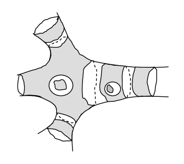
Figure 6. A $\mathcal{S}^{\star}$-piece $S^{\star}$ with boundary $\partial S^{\star}=\gamma\cup\gamma_{1}\cup\gamma_{2}\cup\gamma_{3}$. Here, $E^{\star}_{0}$ is the $\mathcal{E}^{\star}_{ess}$-piece parallel to $S^{\star}$, $E^{\star}_{1}$ and $E^{\star}_{2}$ are two $\mathcal{E}^{\star}_{A}$-pieces between $\gamma$ and $\beta_{\gamma}$.

6.5. $\lambda(\Gamma,f)<1$ implies Grötzsch inequality

For any $\mathcal{S}^{\star}$-piece $S^{\star}$ and any $\gamma\in\partial_{1}(S^{\star})$, let $A_{S^{\star}}^{\gamma}$ be the annulus bounded by $\gamma$ and $\beta_{\gamma}$. By the construction of $\Phi^{t}_{S^{\star}},\Psi^{t}_{S^{\star}}:\mathbb{\overline{C}}(S^{\star})\rightarrow\mathbb{\overline{C}}$, both $\Phi^{t}_{S^{\star}}(\gamma)$ and $\Psi^{t}_{S^{\star}}(\beta_{\gamma})$ are equipotentials. We denote the annulus between $\Phi^{t}_{S^{\star}}(\gamma)$ and $\Psi^{t}_{S^{\star}}(\beta_{\gamma})$ by $A^{t}(S^{\star},\gamma)$. It’s obvious that

$${\rm mod}(A^{t}(S^{\star},\gamma))=\varpi(\Phi^{t}_{S^{\star}}(\gamma))-\varpi(\Psi^{t}_{S^{\star}}(\beta_{\gamma}))=\sigma_{t}(\gamma)-\frac{\sigma_{t}(f(\beta_{\gamma}))}{\deg(f|_{\beta_{\gamma}})}.$$

Then we have the following

Lemma 6.6 (Large parameter implies Grötzsch inequality).

When $t$ is large enough, for any $\mathcal{S}^{\star}$-piece $S^{\star}$ and any $\gamma\in\partial_{1}(S^{\star})$, we have

$$\sum_{\mathcal{E}^{\star}_{A}\ni E^{\star}\subset\overline{A_{S^{\star}}^{\gamma}}}{\rm mod}(\Psi_{E^{\star}}^{t}(A(E^{\star})))<{\rm mod}(A^{t}(S^{\star},\gamma)),$$

where the sum is taken over all the $\mathcal{E}^{\star}_{A}$-pieces contained in $\overline{A_{S^{\star}}^{\gamma}}$.

Proof.

It suffices to show that when $t$ is large enough,

$$\sum_{\mathcal{E}^{\star}_{A}\ni E^{\star}\subset\overline{A_{S^{\star}}^{\gamma}}}\Bigg{(}\frac{\sigma_{t}(f(\alpha_{E^{\star}}))}{\deg(f|_{\alpha_{E^{\star}}})}+\frac{\sigma_{t}(f(\beta_{E^{\star}}))}{\deg(f|_{\beta_{E^{\star}}})}+C(E^{\star})\Bigg{)}+\frac{\sigma_{t}(f(\beta_{\gamma}))}{\deg(f|_{\beta_{\gamma}})}<t\cdot\rho(S_{\gamma},\pi(\gamma))\cdot v(\pi(\gamma)),$$

where $\alpha_{E^{\star}}$ and $\beta_{E^{\star}}$ are the boundary curves of $E^{\star}$, homotopic to $\gamma$ in $\mathbb{\overline{C}}-P$.

One can verify that

$$\sum_{\mathcal{E}^{\star}_{A}\ni E^{\star}\subset\overline{A_{S^{\star}}^{\gamma}}}\Bigg{(}\frac{\sigma_{t}(f(\alpha_{E^{\star}}))}{\deg(f|_{\alpha_{E^{\star}}})}+\frac{\sigma_{t}(f(\beta_{E^{\star}}))}{\deg(f|_{\beta_{E^{\star}}})}\Bigg{)}+\frac{\sigma_{t}(f(\beta_{\gamma}))}{\deg(f|_{\beta_{\gamma}})}=\sum_{\beta\in\Sigma^{\star}}\sum_{\alpha\sim\gamma,\alpha\subset S^{\star}_{\gamma}}\frac{\sigma_{t}(\beta)}{{\rm deg}(f:\alpha\rightarrow\beta)}.$$

Since $\Sigma^{\star}=\Gamma_{0}^{\star}\cup\Gamma^{\star}$, we can decompose the sum into two parts:

$$I=\sum_{\beta\in\Gamma^{\star}}\sum_{\alpha\sim\gamma,\alpha\subset S^{\star}_{\gamma}}\frac{\sigma_{t}(\beta)}{{\rm deg}(f:\alpha\rightarrow\beta)},\ II=\sum_{\beta\in\Gamma_{0}^{\star}}\sum_{\alpha\sim\gamma,\alpha\subset S^{\star}_{\gamma}}\frac{\sigma_{t}(\beta)}{{\rm deg}(f:\alpha\rightarrow\beta)}.$$

It follows from the proof of Lemma 6.2 that $I\leq t\omega(\gamma)$, where

$$\omega(\gamma):=\frac{\rho(S_{f(\gamma)},\pi({f(\gamma)}))v(\pi({f(\gamma)}))}{{\rm deg}(f|_{\gamma})}+\sum_{\delta\in\Gamma}\sum_{\pi(\gamma)\sim\alpha\subset{S}_{\gamma}\setminus{\pi(\gamma)}}\frac{v(\delta)}{{\rm deg}(f:\alpha\rightarrow\delta)},$$

if $f(\gamma)\in\Gamma^{\star}$ (or equivalently $\gamma\in\Gamma_{2}^{\star}\cup\Gamma_{3}^{\star}\cup\cdots$); and

$$\omega(\gamma):=\sum_{\delta\in\Gamma}\sum_{\pi(\gamma)\sim\alpha\subset{S}_{\gamma}\setminus{\pi(\gamma)}}\frac{v(\delta)}{{\rm deg}(f:\alpha\rightarrow\delta)},$$

if $f(\gamma)\in\Gamma_{0}^{\star}$ (or equivalently $\gamma\in\Gamma_{1}^{\star}$).

For the second term, we have

$$II\leq\sum_{A\in\mathcal{A}}\sum_{\alpha\in f^{-1}(\Gamma_{0})\setminus\Gamma_{0}}\frac{{\rm mod}(A)}{\deg(f|_{\alpha})},$$

where $\mathcal{A}$ is the collection of all rotation annuli of $(f,P)$.

So if we choose $t$ large enough such that for any $\gamma\in\cup_{S^{\star}\in\mathcal{S}^{\star}}\partial_{1}(S^{\star})$,

$$\sum_{E^{\star}\in\mathcal{E}^{\star}_{A}}C(E^{\star})+\sum_{A\in\mathcal{A}}\sum_{\alpha\in f^{-1}(\Gamma_{0})\setminus\Gamma_{0}}\frac{{\rm mod}(A)}{\deg(f|_{\alpha})}<t\Big{(}\rho(S_{\gamma},\pi(\gamma))\cdot v(\pi(\gamma))-\omega(\gamma)\Big{)},$$

then the conclusion follows (notice that by the choice of the number $\rho$, we have $\rho(S_{\gamma},\pi(\gamma))\cdot v(\pi(\gamma))-\omega(\gamma)>0$ for all $\gamma\in\Gamma^{\star}$). ∎

6.6. Proof of the sufficiency of Theorem 5.1 ($\Gamma\neq\emptyset$)

Now, we are ready to complete the proof of Theorem 5.1. Here is a fact used in the proof, which is equivalent to the Grötzsch inequality. Let $A,B\subset\mathbb{\overline{C}}$ be two annuli. We say that $B$ can be embedded into $A$ essentially and holomorphically if there is a holomorphic injection $\phi:B\rightarrow A$ such that $\phi(B)$ separates the two boundary components of $A$.

Fact Let $A,A_{1},\cdots,A_{n}\subset\mathbb{\overline{C}}$ be annuli, then $A_{1},\cdots,A_{n}$ can be embedded into $A$ essentially and holomorphically such that the closures of the images of $A_{i}$’s are mutually disjoint if and only if

$$\sum_{i=1}^{n}{\rm mod}(A_{i})<{\rm mod}(A).$$

Proof of the sufficiency of Theorem 5.1, assuming $\Gamma\neq\emptyset$. The idea of the proof is to glue the holomorphic models in a suitable fashion along the stable multicurve $\Gamma$.

Recall that for each $\mathcal{S}^{\star}$-piece $S^{\star}$, we use $S$ to denote the $\mathcal{S}$-piece that contains $S^{\star}$. For each curve $\gamma\in\Sigma$, $A^{\gamma}$ is the annular neighborhood of $\gamma$ chosen at the beginning of Section 6.3. The collection of all rotation annuli of $(f,P)$ is still denoted by $\mathcal{A}$.

For each $\mathcal{S}^{\star}$-piece $S^{\star}$, we extend $\Phi_{S^{\star}}^{t}:S^{\star}\rightarrow\Phi_{S^{\star}}^{t}(S^{\star})$ to a quasi-conformal homeomorphism $\Phi_{S}:{S}\rightarrow\Phi_{S}(S)$ such that $\Phi_{S}$ is holomorphic in $(S-S^{\star})\cap(\cup\mathcal{A})$.

We first choose $t$ large enough such that Lemma 6.6 holds. This means, one can embedded $\Psi_{E^{\star}}^{t}(E^{\star})$ holomorphically into the interior of $\Phi_{S}(S)$ for each $\mathcal{E}^{\star}_{A}$-piece $E^{\star}$ contained in $S$ according to the original order of their non-peripheral boundary curves so that the embedded images are mutually disjoint. In other words, there is a quasi-conformal homeomorphism $\psi_{S}:S\rightarrow\Phi_{S}(S)$ such that

$\bullet$ $\psi_{S}|_{\partial S}=\Phi_{S}|_{\partial S}$ and $\psi_{S}$ is isotopic to $\Phi_{S}$ rel $\partial S\cup(S\cap P)$. Moreover, $\psi_{S}|_{S\cap(\cup\mathcal{A})}=\Phi_{S}|_{S\cap(\cup\mathcal{A})}$.

$\bullet$ $\psi_{S}|_{E_{S^{\star}}}=\Psi_{S^{\star}}^{t}|_{E_{S^{\star}}}$, where $E_{S^{\star}}$ is the unique $\mathcal{E}^{\star}$-piece parallel to $S^{\star}$.

$\bullet$ For each curve $\gamma\in\partial_{1}(S)$, $\Phi_{S}(S\cap A^{\gamma})=\psi_{S}(S\cap A^{\gamma})$.

$\bullet$ For every $\mathcal{E}^{\star}_{A}$-piece $E^{\star}$ with $E^{\star}\subset S$, the map $\Psi_{E^{\star}}^{t}\circ\psi_{S}^{-1}$ is holomorphic in $\psi_{S}(E^{\star})$.

We define a subset $\mathcal{E}_{A}$ of $\mathcal{E}$ by $\mathcal{E}_{A}=\{E;E^{\star}\in\mathcal{E}^{\star}_{A}\}$. Let $\mathcal{D}(S)$ be the collection of all disk components of $S-E_{S}\cup(\cup_{\mathcal{E}_{A}\ni E\subset S}E)$, here $E_{S}$ is the unique $\mathcal{E}$-piece parallel to $S$. For each $D\in\mathcal{D}(S)$, we construct a quasi-conformal homeomorphism $\zeta_{D}:D\rightarrow\psi_{S}(D)$, whose Beltrami coefficient satisfies

$$\mu_{\zeta_{D}}(z)=\sum_{\mathcal{E}\ni E\subset D}\chi_{E}(z)\mu_{\Phi_{f(E)}\circ f}(z),$$

here the sum is taken over all $\mathcal{E}$-pieces contained in $D$. We further require $\zeta_{D}(p)=\psi_{S}(p)$ if $D$ contains a marked point $p\in P$.

Let $\Gamma_{S}$ be the collection of all boundary curves of $\cup_{D\in\mathcal{D}(S)}D$. For each $\gamma\in\Gamma_{S}$, notice that $f(\gamma)\in\Sigma$. Let $A^{\gamma}$ be the component of $f^{-1}(A^{f(\gamma)})$ containing $\gamma$. It’s obvious that $A^{\gamma}$ is an annular neighborhood of $\gamma$. We define a quasi-conformal homeomorphism $\Psi_{S}:S\rightarrow\Phi_{S}(S)$ by

$$\Psi_{S}(z)=\begin{cases}\zeta_{D}(z),\ \ &z\in D,D\in\mathcal{D}(S),\\ \psi_{S}(z),\ \ &z\in S-(\cup_{D\in\mathcal{D}(S)}D)\cup(\cup_{\gamma\in\Gamma_{S}}A^{\gamma}),\\ q.c\ interpolation,\ \ &z\in\cup_{\gamma\in\Gamma_{S}}A^{\gamma}-\cup_{D\in\mathcal{D}(S)}D.\end{cases}$$

The map $\Psi_{S}$ satisfies:

$\bullet$ $\Psi_{S}|_{\partial S}=\Phi_{S}|_{\partial S}$ and $\Psi_{S}$ is isotopic to $\Phi_{S}$ rel $\partial S\cup(S\cap P)$. Moreover, $\Psi_{S}|_{S\cap(\cup\mathcal{A})}=\Phi_{S}|_{S\cap(\cup\mathcal{A})}$.

$\bullet$ For every $\mathcal{E}^{\star}_{ess}\cup\mathcal{E}^{\star}_{A}$-piece $E^{\star}\subset S$, the map $\Phi_{f(E)}\circ f\circ\Psi_{S}^{-1}$ is holomorphic in $\Psi_{S}(E^{\star})$.

$\bullet$ For every $\mathcal{E}$-piece ${E}\subset\cup_{D\in\mathcal{D}(S)}D$, the map $\Phi_{f(E)}\circ f\circ\Psi_{S}^{-1}$ is holomorphic in $\Psi_{S}(E)$.

Now, we define a quasi-conformal map $\Theta:\mathbb{\overline{C}}\rightarrow\mathbb{\overline{C}}$ by $\Theta|_{S}=\Psi_{S}^{-1}\circ\Phi_{S}$ for all $S\in\mathcal{S}$. It’s obvious that $\Theta$ is isotopic to the identity map rel $P$. Moreover, for each curve $\gamma\in\Gamma$, we have $\Theta(\gamma)=\gamma$ and $A^{\gamma}\subset\Theta^{-1}(A^{\gamma})$. Let $\Phi:\mathbb{\overline{C}}\rightarrow\mathbb{\overline{C}}$ be the quasi-conformal map whose Beltrami coefficient satisfies

$$\mu_{\Phi}(z)=\sum_{S\in\mathcal{S}}\chi_{S}(z)\mu_{\Phi_{S}}(z),\ z\in\mathbb{\overline{C}}.$$

Set $\Psi=\Phi\circ\Theta^{-1}$. Then $(f,P)$ is q.c-equivalent to the Herman map $(g,Q):=(\Phi\circ f\circ\Psi^{-1},\Phi(P))$ via $(\Phi,\Psi)$.

One can verify that $g$ is holomorphic outside $X:=\Psi(\cup_{\gamma\in\Gamma\cup(\cup_{S\in\mathcal{S}}\Gamma_{S})}A^{\gamma})$. To see this, notice that if $E^{\star}\in\mathcal{E}^{\star}_{ess}\cup\mathcal{E}^{\star}_{A}$ and $E^{\star}$ is contained in some $\mathcal{S}$-piece $S$, then the decomposition

$$g|_{\Psi(E^{\star})}=(\Phi\circ\Phi_{f(E)}^{-1})\circ(\Phi_{f(E)}\circ f\circ\Psi_{S}^{-1})\circ(\Phi_{S}\circ\Phi^{-1})|_{\Psi(E^{\star})}$$

implies that $g$ is holomorphic in $\Psi(E^{\star})$ since each factor is holomorphic. If $E\in\mathcal{E}$ and $E\subset D\in\mathcal{D}(S)$, then

$$g|_{\Psi(E)}=(\Phi\circ\Phi_{f(E)}^{-1})\circ(\Phi_{f(E)}\circ f\circ\zeta_{D}^{-1})\circ(\Phi_{S}\circ\Phi^{-1})|_{\Psi(E)},$$

so $g$ is holomorphic in $\Psi(E)$.

The last step is to apply the quasi-conformal surgery. For each curve $\gamma\in\Gamma$, let $\iota(\gamma)$ be the first integer $p\geq 1$ such that $f^{p}(\gamma)\in\Gamma_{0}$ and $L=\max_{\gamma\in\Gamma}\iota(\gamma)$. One may verify by induction that for any $j\geq 1$,

$$g^{-j}(\Psi(\cup\mathcal{A}))=\Psi((\Theta\circ f)^{-j}(\cup\mathcal{A}))\supset\Psi(\cup_{\gamma\in\Gamma,\iota(\gamma)\leq j}A^{\gamma}).$$

In particular, $g^{-L-1}(\Psi(\cup\mathcal{A}))\supset X$. Let $\sigma_{0}$ be the standard complex structure in $\mathbb{\overline{C}}$. Define a $(g,Q)$-invariant complex structure $\sigma$ by

$$\sigma=\begin{cases}(g^{k})^{*}(\sigma_{0}),\ \ &\text{ in }g^{-k}(\Psi(\cup\mathcal{A}))\setminus g^{-k+1}(\Psi(\cup\mathcal{A})),\ k\geq 1,\\ \sigma_{0},\ \ &\text{ in }\mathbb{\overline{C}}-\cup_{k\geq 1}(g^{-k}(\Psi(\cup\mathcal{A}))\setminus g^{-k+1}(\Psi(\cup\mathcal{A}))).\end{cases}$$

Since $(g,Q)$ is holomorphic outside $X$, the Beltrami coefficient $\mu$ of $\sigma$ satisfies $\|\mu\|_{\infty}<1$. By Measurable Riemann Mapping Theorem, there is a quasi-conformal map $\zeta:\mathbb{\overline{C}}\rightarrow\mathbb{\overline{C}}$ such that $\zeta^{*}(\sigma_{0})=\sigma$. Let $R=\zeta\circ g\circ\zeta^{-1}$, then $R$ is a rational map and $(f,P)$ is q.c-equivalent to $(R,\zeta\circ\Phi(P))$ via $(\zeta\circ\Phi,\zeta\circ\Psi)$. $\Box$

7. Analytic part: renormalizations

In this section, we discuss rational-like maps, renormalizations of rational maps and prove Theorem 2.9.

7.1. Rational-like maps

A rational-like map $g:U\rightarrow V$ is a proper and holomorphic map between two multi-connected domains such that $\overline{U}\subset V\subset\mathbb{\overline{C}}$ and the complementary set $\mathbb{\overline{C}}-{X}$ of $X\in\{U,V\}$ consists of finitely many topological disks. In our discussion, we always assume $V\neq\mathbb{\overline{C}}$ and the degree of $g$ is at least two. The filled Julia set is defined by $K(g)=\bigcap_{n\geq 1}g^{-n}(V)$, the Julia set is defined by $J(g)=\partial K(g)$. The Julia set $J(g)$ is not necessarily connected even if $K(g)$ is connected (but in the polynomial-like case, the connectivity of $K(g)$ always implies the connectivity of $J(g)$ by the Maximum Modulus Principle).

Two rational-like maps $g_{1}$ and $g_{2}$ are hybrid equivalent if there is a quasi-conformal conjugacy $\phi$ between $g_{1}$ and $g_{2}$, defined in a neighborhood of $K(g_{1})$, such that $\overline{\partial}\phi=0$ on $K(g_{1})$. We call $\phi$ a hybrid conjugacy between $g_{1}$ and $g_{2}$. These definitions are simply the generalizations of Douady-Hubbard’s definitions for polynomial-like maps [DH3].

The following is an analogue of Douady-Hubbard’s straightening theorem:

Theorem 7.1 (Straightening theorem).

Let $g:U\rightarrow V$ be a rational-like map of degree $d\geq 2$, then

1. The map $g$ is hybrid equivalent to a rational map $R$ of degree $d$.

2. If $K(g)$ is connected, then $g$ is hybrid equivalent to a rational map $R$ of degree $d$, which is postcritically finite outside $\phi(K(g))$. Here $\phi$ is the hybrid conjugacy. Such $R$ is unique up to Möbius conjugation.

Remark 7.2.

1. A rational-like map $g:U\rightarrow V$ can be hybrid equivalent to a rational map of degree greater than $d$.

2. In the second statement of Theorem 7.1, if we do not require the degree of $R$, then $R$ may be not unique up to Möbius conjugation even if $R$ is postcritically finite outside $\phi(K(g))$. For example, we can consider the McMullen map: $f_{\lambda}(z)=z^{n}+\lambda/z^{n}$ with $n\geq 3$. Here $\lambda$ is a complex parameter such that $f_{\lambda}$ is postcritically finite and the Julia set is a Sierpinski curve. We denote by $B_{\lambda}$ the immediate attracting basin of $\infty$. In this case, $f_{\lambda}$ is strictly expanding on $\partial B_{\lambda}$. There is an annular neighborhood $A$ of $\partial B_{\lambda}$ such that $f_{\lambda}|_{A}:A\rightarrow f_{\lambda}(A)$ is a rational-like map. It is hybrid equivalent to the power map $z\mapsto z^{n}$, with degree lower than that of $f_{\lambda}$. More details can be found in [QWY].

3. If $K(g)$ is connected and $\mathbb{\overline{C}}-K(g)$ consists of two components, then there are two annuli $U^{\prime},V^{\prime}$ such that $K(g)\Subset U^{\prime}\Subset V^{\prime}\Subset V$ and the restriction $g|_{U^{\prime}}:U^{\prime}\rightarrow V^{\prime}$ is a rational-like map. In this case, $K(g)$ is a quasi-circle.

Proof.

1. The proof is a standard surgery procedure. By shrinking $V$ a little bit, we may assume that each boundary curve of $U$ and $V$ is a quasi-circle. We then extend $g:U\rightarrow V$ to a quasi-regular branched covering $G:\mathbb{\overline{C}}\rightarrow\mathbb{\overline{C}}$ such that $G$ is holomorphic in $\mathbb{\overline{C}}-\overline{V}$ and $G$ maps each component $U_{k}$ of $\mathbb{\overline{C}}-{U}$ onto a connected component $V_{j}$ of $\mathbb{\overline{C}}-{V}$, with degree equal to $\deg{(g|_{\partial U_{k}})}$. Such extension keeps the degree. By pulling back the standard complex structure $\sigma_{0}$ on $\mathbb{\overline{C}}-{V}$ via $G$, we get a $G$-invariant complex structure

$$\sigma=\begin{cases}(G^{k})^{*}(\sigma_{0}),\ \ &\text{ in }G^{-k}(\mathbb{\overline{C}}-{V}),\ k\geq 1,\\ \sigma_{0},\ \ &\text{ in }K(g).\end{cases}$$

The Beltrami coefficient $\mu$ of $\sigma$ satisfies $\mu|_{K(g)}=0$ and $\|\mu\|_{\infty}<1$. Let $\phi$ solve the Beltrami equation $\overline{\partial}\phi=\mu\partial\phi$. Then $R=\phi\circ G\circ\phi^{-1}$ is a rational map and $\phi$ is a hybrid conjugacy between $g$ and $R$.

2. By a hole-filling process (see Theorem 5.1 in [CT1], or Proposition 6.5.1 in [W]), we can find a suitable restriction $g|_{U^{\prime}}:U^{\prime}\rightarrow V^{\prime}$ of $g$ with $K(g)\Subset U^{\prime}\Subset V^{\prime}\Subset V$ such that

a). All postcritical points of $g|_{U^{\prime}}$ in $V^{\prime}$ are contained in $K(g)$.

b). Each connected component of $V^{\prime}-\overline{U^{\prime}}$ is either an annulus or a disk.

Note that such $V^{\prime}$ can be chosen arbitrarily close to the filled Julia set $K(g)$. (To see this, one may replace $V^{\prime}$ by $g^{-k}(V^{\prime})$ for some large $k$, and a), b) still holds.)

In this way, each component $U_{i}$ of $\mathbb{\overline{C}}-\overline{U^{\prime}}$ either is contained in $V^{\prime}$ or contains a unique component $V_{j}$ of $\mathbb{\overline{C}}-\overline{V^{\prime}}$. In the former case, we mark a point $p\in U_{i}$ and get a marked disk $(U_{i},p)$; in the latter case, we mark a point $p\in V_{j}$, and get two marked disks $(V_{j},p)$ and $(U_{i},p)$. We extend $g|_{U^{\prime}}$ to a quasi-regular branched covering $G:\mathbb{\overline{C}}\rightarrow\mathbb{\overline{C}}$ such that

1). For each component $U_{i}$ of $\mathbb{\overline{C}}-\overline{U^{\prime}}$, $G$ maps the marked disk $(U_{i},p)$ to the marked disk $(V_{k},q)$, where $V_{k}$ is the component of $\mathbb{\overline{C}}-\overline{V^{\prime}}$ whose boundary is $g(\partial U_{i})$. We require that $G(p)=q$ and the local degree of $G$ at $p$ is equal to $\deg{(g|_{\partial U_{i}})}$.

2). We further require that $G$ is holomorphic in $\mathbb{\overline{C}}-\overline{V^{\prime}}$.

By pulling back the standard complex structure on $\mathbb{\overline{C}}-{V^{\prime}}$, we can get a $G$-invariant complex structure whose Beltrami coefficient $\mu$ satisfies $\mu|_{K(g)}=0$ and $\|\mu\|_{\infty}<1$. Let $\phi$ solve the Beltrami equation $\overline{\partial}\phi=\mu\partial\phi$. Then $R=\phi\circ G\circ\phi^{-1}$ is a rational map, postcritically finite outside $\phi(K(g))$, as required.

To prove the uniqueness, we need investigate some mapping properties of $R$, a rational map of degree $d$, to which $g|_{U^{\prime}}$ is hybrid equivalent via $\phi$, and postcritically finite outside $\phi(K(g))$. We assume $V^{\prime}$ is sufficiently close to $K(g)$ so that $\phi$ is defined on $V^{\prime}$. Then $g|_{U^{\prime}}$ induces a suitable restriction $R|_{\phi(U^{\prime})}$. Let $\mathcal{X}_{1}$ be the collection of all components of $\mathbb{\overline{C}}-\phi(K(g))$ which intersect with the boundary curves of $\phi(V^{\prime})$ and $\mathcal{X}_{2}$ be the collection of all components of $\mathbb{\overline{C}}-\phi(K(g))$ which intersect with the boundary curves of $\phi(U^{\prime})$. It’s obvious that $\mathcal{X}_{1}\subset\mathcal{X}_{2}$. Since the degree of $R$ is equal to $d$ (this is very important), we have that

$$\{U{\text{\ }is\ a\ component\ of\ }R^{-1}(X);X\in\mathcal{X}_{1}\}=\mathcal{X}_{2}.$$

Thus for each $X\in\mathcal{X}_{2}$, $R(X)\in\mathcal{X}_{2}$. This implies that each $X\in\mathcal{X}_{2}$ is eventually periodic under the map $R$. Suppose $X\in\mathcal{X}_{2}$ is $R$-periodic, with period $p$. Since $R$ is poscritically finite outside $\phi(K(g))$, $R^{p}|_{X}:X\rightarrow X$ is proper and each critical point in $X$ has finite orbit. Thus $R^{p}|_{X}$ is conformally conjugate to $z\mapsto z^{d}$, where $d={\deg}(R^{p}|_{X})\geq 2$ (see [DH1] Lemma 4.1 for a proof of this fact). It follows that for all $X\in\mathcal{X}_{2}$, the proper map $R|_{X}:X\rightarrow R(X)$ has only one possible critical point, which is eventually mapped to a superattracting cycle. Base on these observations, we are now ready to prove the uniqueness part of the theorem.

Suppose that $R_{1}$ and $R_{2}$ are two rational maps of degree $d$, both are hybrid equivalent to $g|_{U^{\prime}}$ and poscritically finite outside $\phi_{1}(K(g))$ and $\phi_{2}(K(g))$, respectively. Here, $\phi_{i}$ is a hybrid conjugacy between $g|_{U^{\prime}}$ and $R_{i}$, $i=1,2$. We assume that $V^{\prime}$ is sufficiently close to $K(g)$ such that $\phi_{i}$ is defined on $U^{\prime}$. Then $g|_{U^{\prime}}$ induces two restrictions $R_{i}|_{\phi_{i}(U^{\prime})},i=1,2$ and a hybrid conjugacy $\phi=\phi_{2}\circ\phi_{1}^{-1}$ between them. One can construct a pair of quasi-conformal maps $\varphi_{0},\varphi_{1}:\mathbb{\overline{C}}\rightarrow\mathbb{\overline{C}}$ such that

a). $\varphi_{0}\circ R_{1}=R_{2}\circ\varphi_{1}$ on $\mathbb{\overline{C}}$.

b). $\varphi_{0},\varphi_{1}$ are isotopic rel $\phi_{1}(K(g))\cup P_{R_{1}}$ and $\varphi_{0}|_{\phi_{1}(U^{\prime})}=\varphi_{1}|_{\phi_{1}(U^{\prime})}=\phi|_{\phi_{1}(U^{\prime})}$.

c). $\varphi_{0},\varphi_{1}$ are holomorphic and identical in a neighborhood $N$ of all superattracting cycles of $R_{1}$ in $\mathbb{\overline{C}}-\phi_{1}(K(g))$.

Then there is a sequence of quasi-conformal maps $\{\varphi_{n},n\geq 0\}$ such that $\varphi_{n}\circ R_{1}=R_{2}\circ\varphi_{n+1}$ and $\varphi_{n}$ is isotopic to $\varphi_{n+1}$ rel $R_{1}^{-n}(\phi_{1}(U^{\prime})\cup P_{R_{1}}\cup N)$. The quasi-conformal map $\varphi_{n}$ satisfies $\overline{\partial}\varphi_{n}=0$ on $\phi_{1}(K(g))\cup R_{1}^{-n}(N)$. The sequence $\{\varphi_{n}\}$ has a limit quasi-conformal map $\varphi=\lim\varphi_{n}$. Since the Lebesgue measure of $\mathbb{\overline{C}}-\phi_{1}(K(g))\cup R_{1}^{-n}(N)$ tends to zero as $n\rightarrow\infty$, the map $\varphi$ satisfies $\overline{\partial}\varphi=0$ outside a zero measure set. It is in fact a holomorphic conjugacy between $R_{1}$ and $R_{2}$. ∎

7.2. Herman-Siegel renormalization

In this section, we will discuss the renormalizations of Herman rational maps.

Let $(f,P)$ be a Herman rational map. The decomposition procedure in Section 3 yields finitely many $f_{*}$-cycles of $\mathcal{S}$-pieces:

$$S_{\nu}\mapsto f_{*}(S_{\nu})\mapsto\cdots\mapsto f_{*}^{p_{\nu}-1}(S_{\nu})\mapsto f_{*}^{p_{\nu}}(S_{\nu})=S_{\nu},\ \ 1\leq\nu\leq n,$$

where $S_{\nu}$ is a representative of the $\nu$-th cycle and $p_{\nu}$ is the period of $S_{\nu}$.

For $i\in[1,n]$, let $V_{i}=S_{i}$ and $U_{i}$ be the unique component of $f^{-p_{i}}(S_{i})$ parallel to $S_{i}$. The triple $(f^{p_{i}},U_{i},V_{i})$ can be considered as a renormalization of $(f,P)$. In general, $U_{i}$ is not contained in the interior of $V_{i}$ (for example, if some boundary curve $\gamma$ of $V_{i}$ is also a curve in $\Gamma_{0}$, then $\gamma$ is necessarily a boundary curve of $U_{i}$). For this reason, we call $(f^{p_{i}},U_{i},V_{i})$ a Herman-Siegel (‘HS’ for short) renormalization of $(f,P)$.

We should show that $\deg(f^{p_{i}}|_{U_{i}})\geq 2$ for all $i\in[1,n]$. In fact, if $\Gamma=\emptyset$, then all boundary curves of $U_{i}$ are contained in $\Gamma_{0}$ and $U_{i}$ contains at least one critical point of $f^{p_{i}}|_{U_{i}}$. In this case, $\deg(f^{p_{i}}|_{U_{i}})\geq 2$. If $\Gamma\neq\emptyset$, then it follows from Theorem 5.2 that $\lambda(\Gamma,f)<1$. We conclude from Lemma 3.7 that $\deg(f^{p_{i}}|_{U_{i}})\geq 2$.

The filled Julia set $K_{i}$ and Julia set $J_{i}$ of the HS renormalization $(f^{p_{i}},U_{i},V_{i})$ are defined as follows:

$$K_{i}=\cap_{k\geq 0}(f^{p_{i}}|_{U_{i}})^{-k}(U_{i}),\ J_{i}=K_{i}\cap J(f).$$

Note that $\partial K_{i}$ is not a reasonable definition of the Julia set because $\partial K_{i}$ may contain a curve in $\Gamma_{0}$. One may check that $K_{i}$ is connected. Moreover, $J_{i}=\partial K_{i}$ if and only if $\partial(V_{i})\cap\Gamma_{0}=\emptyset$ (in this case, $K_{i}$ is contained in the interior of $V_{i}$). We say that $(f^{p_{i}},U_{i},V_{i})$ is hybrid equivalent to a rational map $R$, if there is a quasi-conformal map $\phi$ defined in an open set $N_{i}$ such that

a). $K_{i}\setminus\partial U_{i}\subset N_{i}\subset U_{i}$;

b). $\overline{\partial}\phi=0$ on $K_{i}\setminus\partial U_{i}$;

c). $\phi\circ f^{p_{i}}=R\circ\phi$ in $(f^{p_{i}}|_{U_{i}})^{-1}(N_{i})\cap N_{i}$.

Theorem 7.3 (Herman-Siegel renormalization).

Let $(f,P)$ be a Herman rational map and $(f^{p_{i}},U_{i},V_{i}),i\in[1,n]$ be all the HS renormalizations defined above. Then

1. For each $i\in[1,n]$, the HS renormalization $(f^{p_{i}},U_{i},V_{i})$ is hybrid equivalent to a rational map $R_{i}$ of degree $\deg(f^{p_{i}}|_{U_{i}})$ which is postcritically finite outside $\phi(K_{i})$. Here $\phi$ is the hybrid conjugacy. Such $R_{i}$ is unique up to Möbius conjugation.

2. The Julia set $J(f)$ has zero Lebesgue measure (resp. carries no invariant line fields) if and only if for each $i\in[1,n]$, the Julia set $J_{i}$ has zero Lebesgue measure(resp. carries no invariant line fields).

Here, we say a rational map $f$ carries an invariant line field if there is a measurable Beltrami differential $\mu=\mu(z){d\bar{z}}/{dz}$ supported on a measurable subset $E\subset J(f)$ such that $E$ has positive measure and $f^{*}\mu=\mu$ a.e. (here, $f^{*}\mu:=\mu(f(w))\frac{\overline{f^{\prime}(w)}d\bar{w}}{f(w)dw}$). The definition can be generalized to $f^{p_{i}}|_{U_{i}}$ similarly.

The proof of the first statement is essentially the same as that of Theorem 7.1, and the straightening map $R_{i}$ is either a Siegel rational map or a Thurston rational map. We omit the details here. The proof of the second statement is based on the following ([Mc2], Theorem 3.9):

Theorem 7.4 (Ergodic or attracting).

Let $f$ be a rational map of degree at least two, then either

$\bullet$ $J(f)=\mathbb{\overline{C}}$ and the action of $f$ on $\mathbb{\overline{C}}$ is ergodic, or

$\bullet$ the spherical distance $d(f^{n}(z),P_{f})\rightarrow 0$ for almost every $z\in J(f)$ as $n\rightarrow\infty$.

Proof of 2 of Theorem 7.3. Let $\mathcal{E}_{ess}\subset\mathcal{E}$ be the collection of all $\mathcal{E}$-pieces (defined in Section 3) that are parallel to the $\mathcal{S}$-pieces. Each element $E\in\mathcal{E}\setminus\mathcal{E}_{ess}$ contains at most one point in the postcritical set $P_{f}$. Moreover, the boundary of $E$ is contained in the Fatou set $F(f)$.

We can define an itinerary map by:

$$iter:\begin{cases}J(f)\rightarrow\mathcal{E}^{\mathbb{N}},\\ z\mapsto(E_{0}(z),E_{1}(z),E_{2}(z),\cdots).\end{cases}$$

where $E_{k}(z)$ is the unique $\mathcal{E}$-piece containing $f^{k}(z)$.

Given a point $z\in J(f)$ with itinerary $iter(z)=(E_{0}(z),E_{1}(z),E_{2}(z),\cdots)$, one can verify that $z\in\cup_{k\geq 0}f^{-k}(J_{1}\cup\cdots\cup J_{n})$ if and only if there is an integer $N$ (depending on $z$) such that for all $k\geq N$, $E_{k}(z)\in\mathcal{E}_{ess}$. Moreover, the set $\cup_{k\geq 0}f^{-k}(J_{1}\cup\cdots\cup J_{n})$ contains all the boundaries of rotation domains, together with their preimages.

This implies that if $z\in J(f)-\cup_{k\geq 0}f^{-k}(J_{1}\cup\cdots\cup J_{n})$, then there exists a sequence of integers $\{n_{j};j\geq 1\}$ such that $E_{n_{j}}(z)\in\mathcal{E}\setminus\mathcal{E}_{ess}$ for all $j\geq 1$. By passing to a subsequence, we assume $\{E_{n_{j}}(z);j\geq 1\}$ satisfies either of the following three properties:

1. $E_{n_{j}}(z)\cap P_{f}=\emptyset$ for all $j\geq 1$.

2. For all $j\geq 1$, $E_{n_{j}}(z)\cap P_{f}\neq\emptyset$ and $E_{n_{j}}(z)$ contains a point in $P_{f}$. This point is contained either in the Fatou set or in the grand orbit of a repelling cycle.

3. For all $j\geq 1$, $E_{n_{j}}(z)\cap P_{f}\neq\emptyset$ and $E_{n_{j}}(z)$ contains a point in $P_{f}$ and the forward orbit of this point accumulates on $P^{\prime}_{f}\cap J(f)$, where $P^{\prime}_{f}$ is the accumulation set of the postcritical set $P_{f}$.

In the first two cases, one may easily check that $\limsup d(f^{n}(z),P_{f})>0$.

In the last case, the set $\{E_{n_{j}}(z);j\geq 1\}$ can be rewritten as $\{E_{1},\cdots,E_{m}\}$, which is a finite subset of $\mathcal{E}\setminus\mathcal{E}_{ess}$. Note that each $E_{k}$ is contained in a disk component or an annular component of $\cup\mathcal{S}-\cup\mathcal{E}_{ess}$, there is an integer $M>0$ such that $f^{-M}(E_{1}\cup\cdots\cup E_{m})\cap P_{f}=\emptyset$. If $\limsup d(f^{n}(z),P_{f})=0$, then there exists a sequence of integers $\{\ell_{j}\}$ such that $d(f^{\ell_{j}}(z),(E_{1}\cup\cdots\cup E_{m})\cap P_{f})\rightarrow 0$ as $j\rightarrow\infty$. It follows that $f^{\ell_{j}-M}(z)\in f^{-M}(E_{1}\cup\cdots\cup E_{m})$ for all large $j$. Since the boundary of each component of $f^{-M}(E_{1}\cup\cdots\cup E_{m})$ is contained in the grand orbits of the Herman rings of $f$, there is a number $\epsilon(z)>0$ such that $d(f^{\ell_{j}-M}(z),P_{f})\geq\epsilon(z)$ for all large $j$. But this contradicts the assumption that $\limsup d(f^{n}(z),P_{f})=0$. So in this case, we also have $\limsup d(f^{n}(z),P_{f})>0$.

Thus, for any $z\in J(f)-\cup_{k\geq 0}f^{-k}(J_{1}\cup\cdots\cup J_{n})$, we have

$$\limsup d(f^{n}(z),P_{f})>0.$$

It follows from Theorem 7.4 that the Lebesgue measure of $J(f)-\cup_{k\geq 0}f^{-k}(J_{1}\cup\cdots\cup J_{n})$ is zero. This means $Leb(J(f))=0$ if and only if for each $k\in[1,n]$, $Leb(J_{k})=0$ (here, we use $Leb$ to denote the Lebesgue measure).

Suppose that $J(f)$ carries an invariant line field. That is, there is a measurable Beltrami differential $\mu$ supported on a positive measure subset $E$ of $J(f)$ such that $f^{*}\mu=\mu$ a.e, and $|\mu|=1$ on $E$. Let $\mu_{k}=\mu|_{J_{k}}$ for $k\in[1,n]$. It follows from the above argument that there exists $\ell\in[1,n]$ with $Leb(J_{\ell}\cap E)>0$. Then the relation $(f^{p_{\ell}}|_{U_{\ell}})^{*}\mu_{\ell}=\mu_{\ell}$ implies that $\mu_{\ell}$ is an invariant line field of $f^{p_{\ell}}|_{U_{\ell}}$. Conversely, suppose that $\mu_{\ell}$ is an invariant line field of $f^{p_{\ell}}|_{U_{\ell}}$, then the Beltrami differential defined by

$$\mu=\mu_{\ell}+\sum_{k\geq 0}((f^{k+1})^{*}\mu_{\ell}-(f^{k})^{*}\mu_{\ell})$$

is an invariant line field of $f$. $\Box$

7.3. Proof of Theorem 2.9

First, we need some lemmas.

Lemma 7.5 (Q.c-equivalence implies q.c-conjugacy).

Let $(f,P)$ and $(g,Q)$ be two HST rational maps. If $(f,P)$ and $(g,Q)$ are q.c-equivalent via a pair of quasi-conformal maps $(\phi_{0},\phi_{1})$, then there is a quasi-conformal map $\phi$, holomorphic in the Fatou set $F(f)$ (probably empty), such that $\phi f=g\phi$.

Proof.

We first deal with the case $J(f)=\mathbb{\overline{C}}$. In that case, $(f,P)$ is postcritically finite. If $(f,P)$ is not a Lattès map, then $(f,P)$ and $(g,Q)$ are Möbius conjugate by Thurston’s theorem. If $(f,P)$ is a Lattès map, then there is a sequence of quasiconformal maps $\phi_{k}$ such that $\phi_{k}f=g\phi_{k+1}$ and $\phi_{k}$ is isotopic to $\phi_{k+1}$ rel $f^{-k}(P)$. Since all $\phi_{k}$ have bounded dilatations and $\overline{\cup_{k\geq 0}f^{-k}(P)}=J(f)=\mathbb{\overline{C}}$, the sequence $\phi_{k}$ converges to a quasi-conformal map which is in fact a conjugacy between $(f,P)$ and $(g,Q)$.

In the following, we assume $J(f)\neq\mathbb{\overline{C}}$. By the definition of q.c-equivalence, $\phi_{0}$ and $\phi_{1}$ are holomorphic and identical in the union of all rotation domains $R_{f}$ of $f$ (if any). If $f$ has a superattracting cycle $z_{0}\mapsto z_{1}\mapsto\cdots\mapsto z_{p-1}\mapsto z_{p}=z_{0}$, then we can modify $\phi_{0}$ and $\phi_{1}$ such that they are holomorphic and identical near the cycle. The modification is as follows:

First, note that for any $0\leq i<p$, $\phi_{0}(z_{i})(=\phi_{1}(z_{i}))$ is a superattracting point of $g$. We can choose a neighborhood $U_{i}$ of $z_{i}$ (resp. $V_{i}$ of $\phi_{0}(z_{i})$), a Böttcher coordinate $B_{i}^{f}:U_{i}\rightarrow\mathbb{D}$ (resp. $B_{i}^{g}:V_{i}\rightarrow\mathbb{D}$), such that the following diagram commutes:

where $d_{i}$ is the local degree of $f$ at $z_{i}$. By suitable choices of the neighborhoods $U_{i}$ and the Böttcher coordinates, we may assume that $\phi_{0}$ and $\phi_{1}$ satisfy $\phi_{0}|_{U_{i}}=\phi_{1}|_{U_{i}}=(B_{i}^{g})^{-1}\circ B_{i}^{f}$. A suitable modification elsewhere guarantees $\phi_{0}f=g\phi_{1}$.

In this way, $\phi_{0}$ and $\phi_{1}$ can be made holomorphic in a neighborhood $N_{SA}$ of all superattracting cycles of $f$ (if any). Then we construct a sequence of q.c maps $\{\phi_{k};k\geq 0\}$ by $\phi_{k}f=g\phi_{k+1}$ so that $\phi_{k}$ is isotopic to $\phi_{k+1}$ rel $f^{-k}(P\cup N_{SA})$. Since $\overline{\cup_{k\geq 0}f^{-k}(P\cup N_{SA})}=\overline{\mathbb{C}}$, the sequence $\phi_{k}$ has a unique limit $\phi$, holomorphic in $\cup_{k\geq 0}f^{-k}(R_{f}\cup N_{SA})=F(f)$, as required. ∎

Now let $M_{1}(J(f),f)$ be the space of invariant line fields carried by $(f,P)$ (we define $M_{1}(J(f),f)$ to be $\{0d\overline{z}/dz\}$ if $(f,P)$ carries no invariant line field). It’s known from McMullen and Sullivan [McS] that $M_{1}(J(f),f)$ is either a single point or a finite-dimensional polydisk. From Lemma 7.5, we have immediately:

Lemma 7.6.

$M_{qc}(f,P)\cong M_{1}(J(f),f)$.

Proof.

By Lemma 7.5, $M_{qc}(f,P)$ is the space of all rational maps (up to Möbius conjugation) q.c-conjugate to $(f,P)$. Moreover, each element of $M_{qc}(f,P)$ corresponds to a unique quasiconformal map $\phi$ up to post-composition a Möbius map so that $\phi$ is holomorphic in the Fatou set $F(f)$. This induces a unique Beltrami differential $\mu_{\phi}\in M_{1}(J(f),f)$. The converse is immediate. ∎

Proof of Theorem 2.9. Let $(f,P)$ be a Herman rational map and $(f^{p_{i}},U_{i},V_{i}),i\in[1,n]$ be all its HS renormalizations defined in Theorem 7.3, whose straightening maps are denoted by $(h_{i},P_{i})$ respectively. We may renumber them so that $(h_{i},P_{i})_{1\leq i\leq m}$ are Siegel rational maps and the rest are Thurston rational maps. Let $M_{1}(J_{i},f^{p_{i}}|_{U_{i}})$ be the space of invariant line fields carried by $(f^{p_{i}},U_{i},V_{i})$. By Theorem 7.3, we have $M_{1}(J_{i},f^{p_{i}}|_{U_{i}})\cong M_{1}(J(h_{i}),h_{i})$. By Lemma 3.7, none of $(h_{i},P_{i})_{m<i\leq n}$ is a Lattès map, thus $M_{1}(J(h_{i}),h_{i})$ is a singleton. To prove Theorem 2.9, it suffices to show

$$M_{1}(J(f),f)\cong M_{1}(J_{1},f^{p_{1}}|_{U_{1}})\times\cdots\times M_{1}(J_{m},f^{p_{m}}|_{U_{m}}).$$

We define $\Phi:M_{1}(J(f),f)\rightarrow M_{1}(J_{1},f^{p_{1}}|_{U_{1}})\times\cdots\times M_{1}(J_{m},f^{p_{m}}|_{U_{m}})$ by $\Phi(\mu)=(\mu|_{J_{1}},\cdots,\mu|_{J_{m}})$. Its inverse is given by

$$\Phi^{-1}(\mu_{1},\cdots,\mu_{m})=\sum_{1\leq\ell\leq m}\Big{(}\mu_{\ell}+\sum_{k\geq 0}((f^{k+1})^{*}\mu_{\ell}-(f^{k})^{*}\mu_{\ell})\Big{)}.$$

Thus $\Phi$ is a isomorphism. $\Box$

8. Corollaries

In this section, we shall prove Theorems 2.10 and 2.11.

Proof of Theorem 2.10. Let $(f,P)$ be an unobstructed Herman map. By Theorem 2.7, there are finitely many unobstructed Siegel maps and Thurston maps, say $(h_{k},P_{k})_{1\leq k\leq n}$, such that the rational realization of $(f,P)$ depends on that of $(h_{k},P_{k})_{1\leq k\leq n}$. We may renumber them so that the first $m$ maps are Siegel maps and the rest are Thurston maps. The decomposition procedure implies that $m\leq n_{RD}(f)+2n_{RA}(f)$. By Lemma 3.7, none of $(h_{k},P_{k})_{m<k\leq n}$ has an orbifold with signature $(2,2,2,2)$. Thus by Thurston’s theorem, all $(h_{k},P_{k})_{m<k\leq n}$ have rational realizations. The rational realization of $(f,P)$ actually depends on that of $(h_{k},P_{k})_{1\leq k\leq m}$. $\Box$

To prove Theorem 2.11, we need the following

Theorem 8.1 (Characterization of Siegel disk, [Z2]).

Let $(S,Z)$ be a Siegel map. Suppose that $(S,Z)$ has only one fixed rotation disk $D$ of bounded type rotation number and $Z\setminus\overline{D}$ is a finite set. Then $(S,Z)$ is c-equivalent to a rational function $(R,Q)$ if and only if $(S,Z)$ has no Thurston obstructions. The rational function $(R,Q)$ is unique up to Möbius conjugation.

Proof of Theorem 2.11. We may assume that $(f,P)$ is unobstructed. By Theorem 2.10, there are two Siegel maps $(h_{1},P_{1}),(h_{2},P_{2})$ such that the rational realization of $(f,P)$ depends on that of $(h_{1},P_{1}),(h_{2},P_{2})$. Each of $(h_{k},P_{k})$ has only one fixed rotation disk $D_{k}$ of bounded type rotation number and $P_{k}\setminus\overline{D_{k}}$ is a finite set. By Theorem 8.1 and Theorem 2.10, $(f,P)$ has an rational realization. The converse follows from Theorem 5.2.

The rigidity part: Note that any two rational realizations of $(f,P)$ are c-equivalent. It’s known in [Z1] that for any rational map, the boundary of a Siegel disk with bounded type rotation number is a quasi-circle. This implies any two rational realizations of $(f,P)$ can be made q.c-equivalent. So $M_{top}(f,P)\cong M_{qc}(f,P)$. It follows from Theorems 2.9 and 8.1 that $M_{qc}(f,P)$ is a singleton. So dose $M_{top}(f,P)$. $\Box$

References

- [Ah] L. V. Ahlfors. Lectures on quasi-conformal mappings , volume 38 of University Lecture Series, Amer. Math. Soc., 2006.
- [ABC] A. Avila, X. Buff and A. Chéritat. Siegel disks with smooth boundaries, Acta Math. 193, no. 1, 1-30, 2004.
- [BFH] B. Bielefield, Y. Fisher, J. H. Hubbard, The classification of critically preperiodic polynomials as dynamical systems. Jour. AMS., 5, 721-762 (1992)
- [Br] D. Brown, Thurston equivalence without postcritical finiteness for a family of polynomial and exponential mappings. Manuscript
- [BCT] X. Buff, G. Cui, L. Tan. Teichmüller spaces and holomorphic dynamics. Handbook of Teichmüller theory, Vol. III, ed. Athanase Papadopoulos, EMS, 2011.
- [C] G. Cui. Dynamics of rational maps, topology, deformation and bifurcation. Preprint. 2002.
- [CT1] G. Cui, L. Tan. A characterization of hyperbolic rational maps, Invent math. DOI 10.1007/s00222-010-0281-8
- [CT2] G. Cui, L. Tan. Hyperbolic-parabolic deformations of rational maps. Manuscript in preparation
- [CJ] G. Cui and Y. Jiang. Geometrically finite and semi-rational branched coverings of the two-sphere, Trans. Amer. Math. Soc. 363 (2011), 2701-2714.
- [DH1] A. Douady and J. H. Hubbard,Etude dynamique des polynômes complexes, Publications mathématiques d’Orsay, 1984.
- [DH2] A. Douady and J. H. Hubbard, A proof of Thurston’s topological characterization of rational functions. Acta Math. 171, 263-297 (1993)
- [DH3] A. Douady and J. H. Hubbard, On the dynamics of polynomial-like mappings, Ann. Sci. École Norm. Sup. 18(1985), 287-343.
- [E] A. L. Epstein,Transersality in holomorphic dynamics (Preliminary Version).
- [Ge] L. Geyer, Sharp bounds for the valence of certain harmonic polynomials. Proc. Amer. Math. Soc. 136 (2008), no. 2, 549-555.
- [Go] S. Godillon, Construction de fractions rationnelles à dynamique prescrite, Thesis, Université de Cergy-Pontoise, 2010.
- [GS] J. Graczyk, G. Swiatek, Siegel disks with critical points in their boundaries, Duke Math. J. Vol 119, no. 1, 2003, 189-196.
- [H1] M.R. Herman, Examples de fractions rationelles ayant une orbite dense sur la sphère de Riemann. Bull. Soc. Math. France 112, 93-142(1984).
- [H2] M.R. Herman, Conjugasion quasi-symétrique des difféomorphismes du cercle et applications aux disques singuliers de Siegel. unpublished Manuscript (1986).
- [HSS] J.H. Hubbard, D. Schleicher, M. Shishikura, Exponential Thurston maps and limits of quadratic differentials. Jour. Amer. Math. Soc. 22, 77-117 (2009)
- [Ma] M. Maskit, On the boundaries of Teichmuller spaces and on Kleinian groups II. Annals of Math. 91(1970), 607-639.
- [Mc1] C. McMullen, The Classification of Conformal Dynamical Systems, Conference ‘Current developments in mathematics’, Cambridge (1995).
- [Mc2] C. McMullen, Complex Dynamics and Renormalization, Ann. of Math. Studies 135, Princeton Univ. Press, Princeton, NJ, 1994.
- [McS] C. McMullen, D. Sullivan Quasiconformal homeomorphisms and dynamics III: The Teichmuller space of a holomorphic dynamical system., Adv. Math. 135(1998), 351-395.
- [M] J. Milnor, Dynamics in One Complex Variable, Vieweg, 1999, 2nd edition, 2000.
- [MT] J. Milnor and W. Thurston, On iterated maps of the interval, in Dynamical systems (College Park, MD, 1986-87), 465-563, Lecture Notes in Math., 1342, Springer, Berlin, 1988.
- [P1] K. Pilgrim, Combinations of Complex Dynamical Systems. Lecture Notes in Mathematics, vol. 1827. Springer, Berlin (2003).
- [P2] K. Pilgrim, Canonical Thurston obstructions. Adv. Math. 158(2001), 154-168.
- [QWY] W. Qiu, X. Wang, Y. Yin. Dynamics of McMullen maps. Adv. Math. 229(2012), 2525-2577.
- [R1] M. Rees, Realization of matings of polynomials as rational maps of degree two. Manuscript (1986)
- [R2] M. Rees, Views of parameter space: topographer and resident, Astérisque 288 (2003)
- [R3] M. Rees, Components of degree two hyperbolic rational maps. Invent. Math., 100 (1990), 357-382.
- [Se] N. Selinger, Thurston’s pullback map on the augmented Teichm ller space and applications. Invent. Math. DOI 10.1007/S00222-011-0362-3
- [S1] M. Shishikura, On the quasi-conformal surgery of rational functions, Ann. Sci. École Norm. Sup. 20(1987) 1-29.
- [S2] M. Shishikura, Trees associated with the configuration of Herman rings, Ergod. Th. Dynam. Sys. 9(1989), p.543-560.
- [ST] M. Shishikura, L. Tan, A family of cubic rationalmaps and matings of cubic polynomials. Exp. Math. 9, 29-53 (2000)
- [Su] D. Sullivan, Quasiconformal homeomorphisms and dynamics I: Solution of the Fatou-Julia problem on wandering domains. Ann. Math. 122(1985), 401-418.
- [T1] L. Tan, Matings of quadratic polynomials. Erg. Th and Dyn. Syst. 12, 589-620 (1992)
- [T2] L. Tan, Branched coverings and cubic Newton maps. Fund. Math. 154(3), 207-260
- [Th1] W.P. Thurston, Geometry and topology of three manifold. Lecture Notes. Princeton University. 1979.
- [Th2] W.P. Thurston, On the combinatorics and dynamics of iterated rational maps. Preprint. 154(3), 207-260
- [W] X. Wang. Dynamics of McMullen maps and Thurston-type theorems for rational maps with rotation domains. Thesis. 2011. available at IMS thesis sever.
- [YZ] M. Yampolsky and S. Zakeri, Mating Siegel quadratic polynomials. Jour. Amer. Math. Soc. 14(1), 25-78, 2000.
- [Z1] G. Zhang, All bounded type Siegel disks of rational maps are quasi-disks, Inventiones Mathematicae, 1-46, 2011.
- [Z2] G. Zhang, Dynamics of Siegel rational maps with prescribed combinatorics. arxiv:0811.3043v1.
- [ZJ] G. Zhang and Y. Jiang, Combinatorial characterization of sub-hyperbolic rational maps. Adv. Math. 221, 1990-2018 (2009)