DESY 12-026
Edinburgh 2011/41
HU-EP-12/05
LPT-Orsay/12-28
MKPH-T-12-08
MS-TP-12-01
SFB/CPP-12-10

Parameters of Heavy Quark Effective Theory
from $N_{\rm f}=2$ lattice QCD

Benoît Blossier^a, Michele Della Morte^b, Patrick Fritzsch^c, Nicolas Garron^d, Jochen Heitger^e, Hubert Simma^f, Rainer Sommer^f, Nazario Tantalo^g,h
a LPT, CNRS et Université Paris-Sud XI, Bâtiment 210, 91405 Orsay Cedex, France
^b Universität Mainz, Institut für Kernphysik, Becherweg 45, 55099 Mainz, Germany
^c Institut für Physik, Humboldt Universität, Newtonstr. 15, 12489 Berlin, Germany
^d Tait institute, School of Physics and Astronomy, University of Edinburgh, Edinburgh, EH9 3JZ, UK
^e Universität Münster, Institut für Theoretische Physik, Wilhelm-Klemm-Str. 9, 48149 Münster, Germany
^f NIC, DESY, Platanenallee 6, 15738 Zeuthen, Germany
^g Dip. di Fisica, Università di Roma ’Tor Vergata’, Via della Ricerca Scientifica 1, I-00133 Rome, Italy
^h INFN, Sez. di Roma ’Tor Vergata’, Via della Ricerca Scientifica 1, I-00133 Rome, Italy
Abstract

We report on a non-perturbative determination of the parameters of the lattice Heavy Quark Effective Theory (HQET) Lagrangian and of the time component of the heavy-light axial-vector current with $N_{\rm f}=2$ flavors of massless dynamical quarks. The effective theory is considered at the $1/m_{\mathrm{h}}$ order, and the heavy mass $m_{\mathrm{h}}$ covers a range from slightly above the charm to beyond the beauty region. These HQET parameters are needed to compute, for example, the b-quark mass, the heavy-light spectrum and decay constants in the static approximation and to order $1/m_{\mathrm{h}}$ in HQET. The determination of the parameters is done non-perturbatively. The computation reported in this paper uses the plaquette gauge action and two different static actions for the heavy quark described by HQET. For the light-quark action we choose non-perturbatively ${\rm O}(a)$-improved Wilson fermions.

Key words: Lattice QCD; Heavy Quark Effective Theory

PACS: 12.38.Gc; 12.39.Hg; 14.40.Nd

1 Introduction

Particle physics enters very exciting times with the start of collecting data at the Large Hadron Collider. Two ways are explored to probe New Physics (NP): either performing a direct search of new particles (e.g. at ATLAS and CMS) from the electroweak scale up to the  TeV scale, or studying rare decays (e.g. at LHCb). The latter give rise to a very rich set of constraints on NP scenarios because they are either mediated by quantum loops, in which high energy particles circulate (that is the case, for instance, in flavor changing neutral currents), or by new current structures (in decays occuring at tree level). B-mesons offer a highly interesting and rich set of (rare) decay channels, such as $b\to s\gamma$, which arises in the standard model only from penguin diagrams, and hence puts strong bounds on NP scenarios. The analysis of inclusive decays such as $B\to X_{s}\gamma$, in particular in the framework of a heavy quark expansion, strongly depends on the knowledge of the b-quark mass, $m_{\rm b}$. In tests of the CKM mechanism, some tensions exist at the moment between $\sin 2\beta$, obtained from the golden mode $B\to J/\Psi K_{s}$, and the CKM matrix element $V_{ub}$ extracted from the $B\to\tau\nu$ leptonic decay [?]. The theoretical input of the latter is the B-meson decay constant $f_{\rm B}$, whose uncertainty is $\sim$ 10%. Currently, there is also a 3-$\sigma$ discrepancy between $V^{B\to\tau\nu}_{ub}$ and $V^{B\to\pi l\nu}_{ub}$. Although it would be surprising if this difference were due to a significant underestimate of $f_{B}$, reducing its error is an important task of lattice QCD.

Lattice QCD will enable us to compute $m_{\rm b}$ and $f_{\rm B}$ with a precision comparable to the one of forthcoming experimental measurements from high luminosity collisions. Nevertheless, a delicate issue for those extractions is how to get a satisfying control on the cut-off effects. Indeed, the Compton length of the b-quark is smaller than the typical finest lattice spacing of simulations in large volumes (used to compute hadronic quantities). Several strategies have been explored in the literature to circumvent this two-scale difficulty [?,?,?,?,?,?,?], see [?] for a recent review. The ALPHA collaboration has proposed to use the framework of Heavy Quark Effective Theory (HQET) [?,?] with a non-perturbative determination of the couplings [?]. Its implementation at the first order in $1/m_{\mathrm{h}}$ has successfully been applied in the quenched approximation [?,?,?,?]. In this paper we will report on our effort to realize our HQET program for $N_{\rm f}=2$ flavors of dynamical quarks, leaving the phenomenological results for forthcoming papers. Here, in particular, we present our determination of the couplings of the effective theory regularized on the lattice.

We use the same notations as in [?]. The HQET Lagrangian density at the leading (static) order is given by

$${\mathscr{L}}_{\rm{stat}}(x)=\overline{\psi}_{\rm h}(x)\,D_{0}\,\psi_{\rm h}(x)\;.$$ (1.1)

A bare quark mass $m_{\rm bare}^{\rm stat}$ has to be added to the energy levels $E^{\rm stat}$ computed with this Lagrangian to obtain the physical ones. For example, the mass of the B-meson in the static approximation is given by

$$m_{\mathrm{B}}=E^{\rm stat}+m_{\rm bare}^{\rm stat}\;.$$ (1.2)

At the classical level $m_{\rm bare}^{\rm stat}$ is simply the (static approximation of the) b-quark mass, $m_{{\rm b}}$, but in the quantized lattice formulation it has to further compensate a divergence, an inverse power of the lattice spacing. Including the $1/m_{\mathrm{h}}$ terms, the HQET Lagrangian reads

$${\mathscr{L}}_{\rm{HQET}}(x) = {\mathscr{L}}_{\rm{stat}}(x)-\omega_{\mathrm{kin}}{\cal O}_{\mathrm{kin}}(x)-\omega_{\mathrm{spin}}{\cal O}_{\mathrm{spin}}(x)\,,$$ (1.3)

$${\cal O}_{\mathrm{kin}}(x) = \overline{\psi}_{\rm h}(x){\bf D}^{2}\psi_{\rm h}(x)\,,\quad{\cal O}_{\mathrm{spin}}(x)=\overline{\psi}_{\rm h}(x){\boldsymbol{\sigma}}\!\cdot\!{\bf B}\psi_{\rm h}(x)\,.$$ (1.4)

At this order, two other unknown parameters appear in the Lagrangian, $\omega_{\mathrm{kin}}$ and $\omega_{\mathrm{spin}}$. Our normalization is such that the classical values of the coefficients are $\omega_{\mathrm{kin}}=\omega_{\mathrm{spin}}=1/(2m_{\mathrm{h}})$. In order to compute the decay constant of a heavy-light meson, one needs the time component of the axial-vector heavy-light current $A_{0}$. At the lowest order of the effective theory, the current is form-identical to the relativistic one. At the $1/m_{\mathrm{h}}$ order, it is enough to add only one term to the static current (because we are only interested in zero-momentum correlation functions, see [?])

$$A^{\rm HQET}_{0}(x) = Z_{\rm A}^{\rm HQET}\,[A^{\rm stat}_{0}(x)+c_{\rm A}^{(1)}A^{(1)}_{0}(x)]\,.$$ (1.5)

In this work we present our non-perturbative determination of the parameters $m_{\rm bare}$ (the generalization of $m_{\rm bare}^{\rm stat}$ to the $1/m_{\mathrm{h}}$ order), $\ln(Z_{\rm A}^{\rm HQET})$, $c_{\rm A}^{(1)}$, $\omega_{\mathrm{kin}}$, and $\omega_{\mathrm{spin}}$ at values of the lattice spacing relevant for the computation of hadronic observables. These parameters allow us to compute, for example, the spectrum of heavy-light mesons and heavy-light decay constants. As we explain in detail in the remainder of this paper, the basic idea is to match, in a small volume, a few observables expanded in the effective theory at finite lattice spacing to their non-perturbative continuum values determined in QCD at a given renormalization group invariant (RGI) heavy quark mass $M$. Collecting the observables in a vector $\Phi$, the matching equation reads

$$\Phi^{\rm HQET}(L,M,a)=\Phi^{\rm QCD}(L,M,0)\;,$$ (1.6)

where $L$ is the space extent of the lattice and $a\to 0$ taken in QCD. Expanding the left hand side of eq. (1.6) at a given order of the inverse heavy quark mass defines a set of HQET parameters. We remind the reader that such an order-by-order treatment [?] is part of the very definition of HQET.

The remainder of the text is organized as follows: in Sect. 2 we summarize the strategy of the computation, in Sect. 3 we give the details of its implementation, the final results can be found in Sect. 4 and Sect. 5 contains our conclusions. Some definitions are relegated to Appendix A, in Appendix B we explain how we tuned the parameters of the simulations and how we performed the renormalization of the QCD quantities, whereas Appendix C contains more technical information about the dynamical fermion runs.

2 Strategy

The computation reported here is done along the lines of [?]. For completeness, we repeat here the basic ingredients but refer the reader to this work for more detailed explanations. We start by the simulations of QCD in a small volume with space extent $L_{1}\approx 0.4{\;\rm fm}$ at four different values of the lattice spacing. We consider $N_{\rm f}=2$ dynamical light quarks that we tune to be massless and a quenched heavy (valence) quark that we simulate at nine different mass values, such that the lightest mass is around the charm mass and the heaviest mass is above the b-quark mass. We compute five renormalized observables that we extrapolate to the continuum

$$\Phi_{i}^{\rm QCD}(L_{1},M,0)=\lim_{a\to 0}\Phi_{i}^{\rm QCD}(L_{1},M,a)\;,\qquad i=1,\ldots,5.$$ (2.7)

The definitions of these observables can be found in [?] and in Appendix A. Here we just mention that $\Phi_{1}$ and $\Phi_{2}$ are finite volume versions of the heavy-light meson mass and the logarithm of the decay constant, respectively (up to kinematic factors). $\Phi_{3}$ is sensitive to the correction of the heavy-light current. Finally, $\Phi_{4}$ and $\Phi_{5}$ are proportional to the kinetic and magnetic corrections, respectively. At the next-to-leading order of the effective theory (i.e. keeping the static and the $1/m_{\mathrm{h}}$ terms) these observables can be expressed in terms of the five parameters discussed in Sect. 1, which we cast into a vector

$$\omega=\left(m_{\rm bare},\,\ln(Z_{\rm A}^{\rm HQET}),\,c_{\rm A}^{(1)},\,\omega_{\mathrm{kin}},\,\omega_{\mathrm{spin}}\right)^{\rm t}\;.$$ (2.8)

More precisely, we write the $1/m_{\mathrm{h}}$ expansion of the observables in the following way:

$$\Phi^{\rm HQET}=\eta+\varphi\,\omega\,\;.$$ (2.9)

The entries of the five-component vector $\eta$ and the five-by-five block-diagonal matrix $\varphi$ are computed by performing a series of numerical simulations of HQET at fixed $L=L_{1}$ and for various lattice spacings $a$. A more explicit form of eq. (2.9) can be found in Appendix A. As anticipated in the introduction, the matching condition that we impose is eq. (1.6) with $L=L_{1}$:

$$\Phi^{\rm HQET}(L_{1},M,a)=\Phi^{\rm QCD}(L_{1},M,0)\;.$$ (2.10)

Solving this equation defines the HQET parameters that we call $\tilde{\omega}(M,a)$

$$\tilde{\omega}(M,a)=\varphi^{-1}(L_{1},a)\Big{(}\Phi^{\rm QCD}(L_{1},M,0)-\eta(L_{1},a)\Big{)}\,.$$ (2.11)

They are the bare couplings of the theory and, as such, can be determined by finite volume matching conditions. By imposing eq. (2.10), the parameters $\tilde{\omega}_{i}$ become functions of $M$, but this heavy quark mass dependence comes entirely from $\Phi^{\rm QCD}$. We then perform another set of simulations of the effective theory in a larger volume of space extent $L_{2}=2L_{1}$. The observables in this volume are then simply obtained by taking the continuum limit of eq. (2.9) in which we insert the parameters $\tilde{\omega}(M,a)$ computed in the previous step:

$$\Phi^{\rm HQET}(L_{2},M,0) = \lim_{a\to 0}\Big{[}\eta(L_{2},a)+\varphi(L_{2},a)\,\tilde{\omega}(M,a)\Big{]}\,.$$ (2.12)

Our formulation of the theory and the non-perturbative determination of $\tilde{\omega}$ guarantees that all divergences, including those of order $1/a\,,\;1/a^{2}$ are cancelled, and that the limit $a\to 0$ exists. Next, the parameters at larger lattice spacings (to be used in large volume) are obtained by inverting eq. (2.9) with $L=L_{2}$,

$$\omega(M,a)=\varphi^{-1}(L_{2},a)\Big{(}\Phi^{\rm HQET}(L_{2},M,0)-\eta(L_{2},a)\Big{)}\;.$$ (2.13)

Finally, in the last step we perform an interpolation (or, in one case, a slight extrapolation) in the inverse bare coupling $\beta=6/g_{0}^{2}$ and obtain $\omega(M,a)$ at exactly those values of the lattice spacing used in our large volume simulations[?].

3 Numerical application

3.1 Continuum extrapolation of the QCD observables

For the QCD simulation, we use the plaquette gauge action and non-perturbatively ${\rm O}(a)$-improved clover fermions [?] for $N_{\rm f}=2$ flavors of dynamical quarks with Schrödinger functional (SF) boundary conditions. We have four different values of the lattice spacing ($\lesssim 0.02{\;\rm fm}$), $\beta$ varying in the range $6.16-6.64$, and the number of lattice points per space direction being $L_{1}/a=20,24,32,40$. The physical volume is kept fixed by imposing for the Schrödinger functional coupling the value $\bar{g}^{2}(L_{1}/2)=2.989$, which corresponds to $L_{1}\approx 0.4{\;\rm fm}$. For each resolution $L_{1}/a$ we tune the dimensionless RGI heavy quark mass such that

$$z=L_{1}M\in\{4\,,6\,,7\,,9\,,11\,,13\,,15\,,18\,,21\}\;.$$ (3.14)

With this choice, $M$ varies approximately from $2{\;\rm GeV}$ to $10{\;\rm GeV}$. More details about their renormalization and about the tuning of the bare coupling and quark masses can be found in Appendix B. For the run parameters we refer the reader to Appendix C. Finally, we also implement tree-level improvement, following exactly the procedure described in Appendix D of [?].

Our strategy for the continuum extrapolation differs somewhat from our previous work. The discretization effects can be important for our heaviest masses. In particular, for the simulations where $L_{1}/a\leq 24$, we might have noticeable contributions of order $(a/L)^{n}$ with $n>2$. We take advantage of the fact that we have various (and quite different) heavy quark masses: since the cut-off effects are smooth functions of $a/L_{1}$ and $z$, we perform a global fit of the form

$$\Phi^{\rm QCD}(L,M,a)=\Phi^{\rm QCD}(L,M,0)\Big{[}1+(a/L_{1})^{2}\;(A+B\,z+C\,z^{2})\Big{]}\;,$$ (3.15)

using only the data points such that $aM<0.7$, as motivated in [?,?]. Note that the two last terms in eq. (3.15) are proportional to $(a/L_{1})\times(aM)$ and ${(aM)^{2}}$. For each observable, $\Phi^{\rm QCD}_{i}$, the parameters of the fit are the nine different values $\Phi_{i}^{\rm QCD}(L,M,0)$ and $A_{i},\,B_{i},\,C_{i}$. As an illustration we show the results of the fit of $\Phi_{1}$ and $\Phi_{2}$ in Fig. 1.

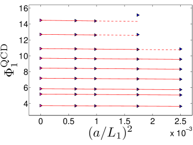
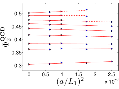
Figure 1: On the top panels we show the continuum extrapolation of two QCD observables where we used a global fit to parametrize the mass dependence of the slopes in $(a/L)^{2}$. The observable shown on the left is proportional to a finite-volume heavy-light meson mass and the one on the right to the logarithm of a finite-volume decay constant. On the lower panels we show the heavy quark mass dependence of these observables ($z=L_{1}M$).

We have checked that different fit ansätze (e.g. adding cubic lattice artefacts) give consistent results for both the central values and the errors, and that results are also compatible with the standard approach where the slope in $(a/L)^{2}$ is not constrained.

3.2 Subtraction of the static part

The effective theory is first simulated in the small volume of space extent $L_{1}$, which is tuned to be the same as in QCD. We use five different lattice spacings, such that $L_{1}/a=6,8,10,12,16$ (but for the continuum extrapolation we discard the coarsest point). The corresponding $\beta$-values lie in the range $5.26-5.96$. For the static quark we use two different lattice actions, HYP1 and HYP2, which are known to lead to small statistical errors [?]. Once again the light quarks are tuned to be massless, both in the valence and in the sea sectors. More details on the simulations can be found in the appendices. This set of simulations serves to compute the quantities $\eta(L_{1},a)$ and $\varphi(L_{1},a)$ in eq. (2.11).

For $i=3,4,5$, the static contributions of $\Phi_{i}$ are $\eta_{i}$. They have a well defined continuum limit and $\eta_{5}=0$. Thus we compute

$$\eta_{i}(L_{1},0)=\lim_{a\to 0}\eta_{i}(L_{1},a)\,,\qquad i=3,4\;,$$ (3.16)

and show the continuum extrapolations in Fig. 2. They are done linearly in $(a/L_{1})^{2}$, which is justified by two reasons: (i) The quantity $\eta_{3}$ contains the time-component of the static axial current; we improve this current using the 1-loop value of $ac_{\rm A}^{\rm stat}$ computed in [?]. This is sufficient since the improvement term has almost no numerical influence: even setting $c_{\rm A}^{\rm stat}=0$ gives compatible results. (ii) The quantity $\eta_{4}$ is constructed from SF boundary-to-boundary correlators, which are already ${\rm O}(a)$-improved in our setup, cf. Appendix C.

Then it is interesting to define the $1/m_{\mathrm{h}}$ contribution to $\Phi_{3,4,5}$,

$$\Phi_{i}^{{(1/m)}}(L_{1},M,0)=\Phi_{i}^{\rm QCD}(L_{1},M,0)-\eta_{i}(L_{1},0)\;,\qquad i=3,4,5,$$ (3.17)

and to study the mass behavior of these quantities, where $\Phi_{4}^{{(1/m)}}(L_{1},M,0)$ and $\Phi_{5}^{{(1/m)}}(L_{1},M,0)$ are a pure kinetic and magnetic correction, respectively. The physical interpretation of $\Phi_{3}^{{(1/m)}}(L_{1},M,0)$ is more subtle and involves the $1/m_{\mathrm{h}}$-correction to the time component of the axial current. Since they are expected to vanish like $1/m_{\mathrm{h}}$ at large $m_{\mathrm{h}}$, any strong deviation from a linear behavior could be interpreted as a contribution from higher-order corrections of the effective theory. One can see from Fig. 3 and Fig. 4 that our results for the heaviest masses are compatible with the expected (linear) leading order behavior in $1/z$.

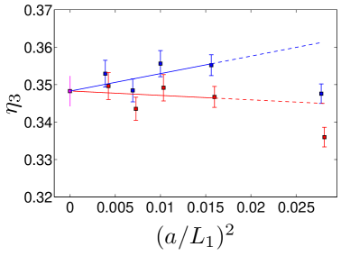
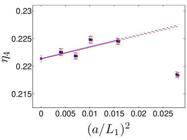
Figure 2: Continuum extrapolation of $\eta_{3}(L_{1},a)$ and $\eta_{4}(L_{1},a)$, which are the static part of $\Phi_{3}(L_{1},M,a)$ and $\Phi_{4}(L_{1},M,a)$ respectively. The two different colors represent the static action: blue for HYP2 and red for HYP1 (slightly shifted to the right).

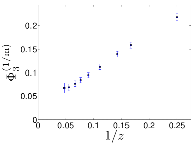
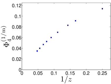
Figure 3: Mass behavior of $\Phi_{3,4}^{{(1/m)}}(L_{1},M,0)$. As explained in the text, these quantities are expected to vanish in the static limit $1/z=0$.

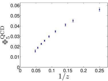
Figure 4: Same as Fig. 3 for the magnetic contribution $\Phi_{5}^{{(1/m)}}(L_{1},M,0)=\Phi_{5}^{\rm QCD}(L_{1},M,0)$.

3.3 Matching in $L_{1}$

With the set of simulations described in the previous section, we have computed $\eta(L_{1},a)$ and $\varphi(L_{1},a)$. Thus the HQET parameters $\tilde{\omega}(M,a)$ can be obtained from eq. (2.11), viz.

$$\tilde{\omega}(M,a)=\varphi^{-1}(L_{1},a)\Big{(}\Phi^{\rm QCD}(L_{1},M,0)-\eta(L_{1},a)\Big{)}\;.$$

However, in practice we split this equation in the following way

$$\tilde{\omega}_{i}(M,a) = \sum_{j=1}^{2}\varphi^{-1}_{ij}(L_{1},a)\Big{(}\Phi_{j}^{\rm QCD}(L_{1},M,0)-\eta_{j}(L_{1},a)\Big{)}$$ (3.18)

$$+ \sum_{j=3}^{5}\varphi^{-1}_{ij}(L_{1},a)\Big{(}\Phi_{j}^{{(1/m)}}(L_{1},M,0)\Big{)}\;,$$

where we have used eq. (3.17). Whether one uses eq. (2.11) or eq. (3.18) to define $\tilde{\omega}(M,a)$ only affects the way we treat the lattice artefacts, but one expects a better precision in the second case. The reason is that the quantities $\eta_{3}$ and $\eta_{4}$ are by far the dominant part of $\Phi_{3}$ and $\Phi_{4}$ (and $\Phi_{5}$ vanishes in the static approximation). As explained in the previous subsection, they are static quantities which extrapolate to the continuum with ${\rm O}(a^{2})$ corrections. On the contrary, $\eta_{1}$ and $\eta_{2}$ are divergent and have to be kept in the combination as in eq. (3.18). They are extrapolated linearly in $a/L_{1}$.

At this point we would like to comment about the separation of the different orders in the effective theory. The situation for the first two observables is different from the others, since $\eta_{1}$ and $\eta_{2}$ do not have a continuum limit. However, the whole matching procedure can be carried out at static order as well. In that case, $\tilde{\omega}_{3}=c_{\rm A}^{(1)}$ is just the improvement coefficient $ac_{\rm A}^{\rm stat}$ which is approximated by perturbation theory. Moreover, the parameters $\tilde{\omega}_{4}$ and $\tilde{\omega}_{5}$ are of order $1/m_{\mathrm{h}}$, and therefore are set to zero. This setup defines the static approximation of the first two observables, $\Phi_{1}^{\rm stat}$ and $\Phi_{2}^{\rm stat}$, with $\varphi={\rm diag}(L_{1},1)$. Performing the matching only for these observables (instead of $\Phi_{i}^{\rm HQET}$ with $i=1,\ldots,5$) allows us to determine the two parameters $m_{\rm bare}^{\rm stat}$ and $\ln(Z_{\rm A}^{\rm stat})$ at static order.

3.4 Evolution to a larger volume $L=L_{2}$

We then consider a set of simulations of HQET in which we use the same parameters as in the previous step (HQET in volume $L_{1}$), but where we double the number of points in each space-time direction. There we compute the quantities $\varphi(L_{2},a)$ and $\eta(L_{2},a)$ with $L_{2}=2L_{1}$. We now have all the ingredients to compute $\Phi(L_{2},M,0)$ using eq. (2.12), but for the reason given above, we use a slightly different version:

$$\Phi_{i}^{\rm HQET}(L_{2},M,0)=\left\{\begin{array}[]{l r}\displaystyle\lim_{a\to 0}\Big{[}\eta_{i}(L_{2},a)+\sum_{j=1}^{5}\varphi_{ij}(L_{2},a)\,\tilde{\omega}_{j}(M,a)\Big{]}\,,&i=1,2\;,\\[8.61108pt] \displaystyle\eta_{i}(L_{2},0)+\lim_{a\to 0}\Big{[}\sum_{j=1}^{5}\varphi_{ij}(L_{2},a)\,\tilde{\omega}_{j}(M,a)\Big{]}\,,&i\geq 3\;,\end{array}\right.$$ (3.21)

Again, the continuum extrapolations of $\eta_{3}$ and $\eta_{4}$ are done linearly in $(a/L_{2})^{2}$, while $\eta_{5}=0$. All other extrapolations are done linearly in $a/L_{2}$ (see the discussions in Sect. 3.2 and Sect. 3.3).

At the static order, the matching procedure at $L_{1}$ and the evolution to $L_{2}$ can be done in the same way as with the five-component vector $\Phi$. The result defines the quantities $\Phi_{i}^{\rm stat}(L_{2},M,0)$ for $i=1,2$, and their continuum extrapolation is shown in Fig. 5. When the matching is performed at the next-to-leading order, we have $\Phi_{i}^{\rm stat}(L_{2},M,0)=\eta_{i}(L_{2},0)$ for $i=3,4,5$ and define the $1/m_{\mathrm{h}}$-contributions as

$$\Phi_{i}^{{(1/m)}}(L_{2},M,0) = \Phi_{i}^{\rm HQET}(L_{2},M,0)-\Phi_{i}^{\rm stat}(L_{2},M,0)\;.$$ (3.22)

Their continuum extrapolations are shown in Fig. 6 and Fig. 7.

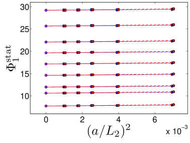
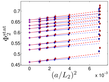
Figure 5: Continuum extrapolation of $\Phi_{1}(L_{2},M,a)$ and $\Phi_{2}(L_{2},M,a)$ in the case where the matching is done in the static approximation. We show the results for the nine different heavy quark masses and the two discretizations HYP1,2. The conventions are the same as in Fig. 1.

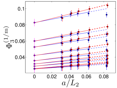
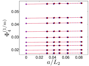
Figure 6: Same as Fig. 5 for the $1/m_{\mathrm{h}}$ contributions $\Phi^{{(1/m)}}_{3}(L_{2},M,a)$ and $\Phi^{{(1/m)}}_{4}(L_{2},M,a)$.

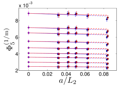
Figure 7: Same as Fig. 5 for $\Phi^{{(1/m)}}_{5}(L_{2},M,a)$.

The parameters $\omega(M,a)$ are computed by the relation analogous to eq. (3.18) in the volume $L_{2}$

$$\omega_{i}(M,a) = \sum_{j=1}^{2}\varphi^{-1}_{ij}(L_{2},a)\Big{(}\Phi_{j}^{\rm HQET}(L_{2},M,0)-\eta_{j}(L_{2},a)\Big{)}$$ (3.23)

$$+ \sum_{j=3}^{5}\varphi^{-1}_{ij}(L_{2},a)\Big{(}\Phi_{j}^{{(1/m)}}(L_{2},M,0)\Big{)}\;.$$

In eq. (3.21) we have chosen to write the evolution of the observables to the volume $L_{2}$ in terms of the HQET couplings $\tilde{\omega}_{i}$. Equivalently we can introduce a matrix of step scaling functions. In order to do that, one substitutes in eq. (3.21) the $\tilde{\omega}_{i}$ by the matching eq. (2.11). One obtains an equation of the following form:

$$\Phi_{i}(L_{2},M,0) = D_{i}\,\Phi_{i}(L_{1},M,0)+\lim_{a/L_{1}\to 0}\,\widehat{\Sigma}_{i}(L_{1},a)$$ (3.24)

$$+ \lim_{a/L_{1}\to 0}\sum_{j=3}^{5}\,\Sigma_{ij}(L_{1},a)\Phi_{j}^{{(1/m)}}(L_{1},M,0)\;,\quad i=1,2\,,$$

$$\Phi_{i}^{{(1/m)}}(L_{2},M,0) = \lim_{a/L_{1}\to 0}\sum_{j=3}^{5}\Sigma_{ij}(L_{1},M,a)\Phi_{j}^{{(1/m)}}(L_{1},M,0)\;,\quad i=3,4,5\,.$$ (3.25)

The explicit definitions of $D,\Sigma$ and $\widehat{\Sigma}$ can be found in [?]. We have implemented the tree-level improvement of these step-scaling functions in order to obtain a smoother approach to the continuum limit. Our results are obtained in this way, but tree-level improvement actually only has a small influence on our results after extrapolation.

4 HQET parameters to be used in large volume simulations

As we have already mentioned in the text and explained in detail in the appendices, the HQET parameters are obtained at five values of the bare coupling $g_{0}^{2}$, which are such that the renormalized coupling $\bar{g}^{2}(L_{2}/4)$ is kept constant for the different ensembles. This is done by setting $\beta$ to some precise values: $\beta=5.2638,5.4689,5.619,5.758,5.9631$. In order to be able to use the HQET parameters in large volume simulations – and make phenomenological predictions – we interpolate (or, in one case, we extrapolate) them to $\beta=5.2,5.3,5.5,5.7$, using a quadratic polynomial in $\beta$. We show this interpolation/extrapolation in Fig. 8. The results are reported in Table 1 for the action HYP2. All errors quoted in this table are statistical (obtained with a standard jackknife procedure), including errors coming from the QCD renormalization constants at finite lattice spacing. There is still an overall relative error contribution of about 0.9% from the quark mass renormalization in QCD, i.e., the factor $h$ in eq. (B.5) of Appendix B, which relates the RGI mass to the SF running mass in the continuum limit. Since in practice this error will only become relevant when the $z$ dependence of the HQET parameters is actually applied to interpolate to the B-meson scale and to extract physical quantities, it is enough to include it then. The complete set of results can be found on our website http://www-zeuthen.desy.de/alpha/, together with the relevant error-correlation matrices. From preliminary studies [?,?], we know that the physical b-quark mass corresponds approximately to $z=13$. For this value of $z$ we display our results for $am_{\rm bare}$ rescaled by $L_{1}/a$ for each value of the lattice spacing in Fig. 9. The parameter $m_{\rm bare}$ absorbs the power divergences present in the binding energy of an heavy-light meson in HQET: a $1/a$ divergence at the static order, and a $1/a^{2}$ divergence at the $1/m_{\mathrm{h}}$ order. As one can see from the figure, $m_{\rm bare}$ is dominated by these power divergences. Clearly, in order to guarantee the existence of the continuum limit, these divergences have to be removed non-perturbatively, which is one of the benefits of our approach.

	$\beta$	5.7	5.5	5.3	5.2
	$z=11$	$0.601(8)$	$0.833(10)$	$1.129(13)$	$1.302(15)$
$am_{\rm bare}^{\mathrm{stat}}$	$z=13$	$0.713(9)$	$0.982(11)$	$1.327(15)$	$1.527(17)$
	$z=15$	$0.821(10)$	$1.127(13)$	$1.518(17)$	$1.746(19)$
	$z=11$	$-0.209(4)$	$-0.201(5)$	$-0.197(5)$	$-0.197(5)$
$\ln(Z_{\rm A}^{\rm stat})$	$z=13$	$-0.191(4)$	$-0.183(5)$	$-0.179(5)$	$-0.178(5)$
	$z=15$	$-0.176(4)$	$-0.169(5)$	$-0.165(5)$	$-0.164(5)$
	$z=11$	$0.058(12)$	$0.377(13)$	$0.740(21)$	$0.937(17)$
$am_{\rm bare}$	$z=13$	$0.236(12)$	$0.582(14)$	$0.985(17)$	$1.207(18)$
	$z=15$	$0.395(13)$	$0.769(15)$	$1.212(18)$	$1.459(20)$
	$z=11$	$-0.212(42)$	$-0.194(37)$	$-0.173(34)$	$-0.162(33)$
$\ln(Z_{\rm A}^{\rm HQET})$	$z=13$	$-0.181(40)$	$-0.166(36)$	$-0.148(32)$	$-0.139(31)$
	$z=15$	$-0.155(41)$	$-0.142(36)$	$-0.127(32)$	$-0.119(31)$
	$z=11$	$-1.00(14)$	$-0.75(12)$	$-0.63(10)$	$-0.60(9)$
$c_{\rm A}^{(1)}/a$	$z=13$	$-0.89(14)$	$-0.68(12)$	$-0.56(10)$	$-0.54(9)$
	$z=15$	$-0.83(15)$	$-0.63(12)$	$-0.52(10)$	$-0.50(9)$
	$z=11$	$0.778(13)$	$0.608(11)$	$0.485(8)$	$0.441(7)$
$\omega_{\mathrm{kin}}/a$	$z=13$	$0.682(13)$	$0.533(10)$	$0.425(8)$	$0.386(7)$
	$z=15$	$0.609(13)$	$0.476(11)$	$0.380(8)$	$0.345(7)$
	$z=11$	$1.626(59)$	$1.284(49)$	$1.041(39)$	$0.956(35)$
$\omega_{\mathrm{spin}}/a$	$z=13$	$1.404(51)$	$1.109(42)$	$0.899(34)$	$0.825(30)$
	$z=15$	$1.236(47)$	$0.976(39)$	$0.791(31)$	$0.727(28)$

Table 1: HQET parameters as a function of the bare coupling for the action HYP2 at $z=11,13,15$. The central value $z=13$ is close to the physical b-quark mass. The first two parameters, $m_{\rm bare}^{\mathrm{stat}}$ and $\ln(Z_{\rm A}^{\rm stat})$, result from the matching at static order, while the remaining entries are the parameter set resulting from the matching of HQET at next-to-leading order.

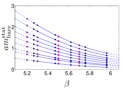
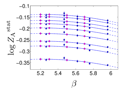
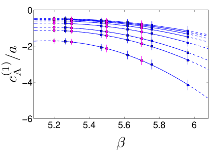
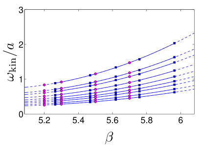
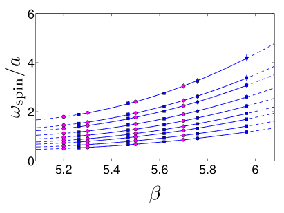
Figure 8: Quadratic fits of HQET parameters in $L_{2}$ as a function of $\beta$. The blue points are the results of the numerical simulations and the magenta points are the interpolated (extrapolated) ones. In this plot we show the results for the HYP2 discretization and for the nine different values of the heavy quark mass.

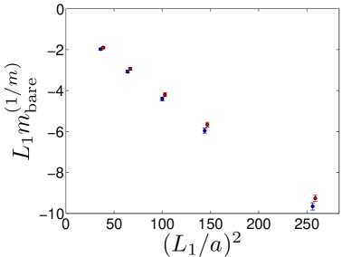
Figure 9: The bare quark mass at the static order and its $1/m_{\mathrm{h}}$ correction, in units of $L_{1}$, for $z=13$ and the two discretizations HYP1,2. These quantities are expected to absorb the power divergences $(1/a)^{n}$, with $n=1$ for the static order and $n=2$ for the $1/m_{\mathrm{h}}$ correction.

Finally, we would like to comment on the size of $1/m_{\mathrm{h}}^{2}$ terms. In our setup, the fermion fields are periodic (in space) up to a phase. As a consequence, the static quantities depend on the choice of one angle, that we call $\theta_{0}$, and the quantities computed at the next-to-leading order of HQET depend on three angles: $\theta_{0},\theta_{1},\theta_{2}$. So far in this work we have considered only what we call the standard choice of $\theta$ angles [?,?], namely $(\theta_{0},\theta_{1},\theta_{2})=(0.5,0.5,1)$. When we change the values of $\theta_{i}$ we change the set of observables, and thereby the matching conditions. The static quantities computed for different values of $\theta$ are thus expected to differ by terms of order $1/m_{\mathrm{h}}$. Once the $1/m_{\mathrm{h}}$ corrections are added, the difference should be of order $1/m_{\mathrm{h}}^{2}$. In general we find no significant $\theta$ dependence for all the HQET parameters $\omega_{i}$ at the next-to-leading order of the effective theory, meaning that the $1/m_{\mathrm{h}}^{2}$ terms are not visible within our statistical precision. As an illustration, we show the spread of our results for $\ln(Z_{\rm A}^{\rm stat})$ and $\ln(Z_{\rm A}^{\rm HQET})$ in Table 2 for the discretization HYP2, $\beta=5.3$, and for $z=13$. Due to statistical correlations, some of the errors on these $1/m_{\mathrm{h}}^{2}$ terms are significantly smaller than our errors for $\ln(Z_{\rm A}^{\rm stat})$ and $\ln(Z_{\rm A}^{\rm HQET})$ themselves, but still no significant $1/m_{\mathrm{h}}^{2}$ term is found.

	$\Delta\ln(Z_{\rm A}^{\rm stat})$	$\Delta\ln(Z_{\rm A}^{\rm HQET})$
$(\theta_{1},\theta_{2})$:		$(0,0.5)$	$(0.5,1)$	$(0,1)$
$\theta_{0}=0.0$	$0.014(2)$	$-0.046(47)$	$-0.001(6)$	$-0.012(14)$
$\theta_{0}=0.5$	$0$	$-0.048(49)$	$0$	$-0.012(12)$
$\theta_{0}=1.0$	$-0.046(2)$	$-0.055(60)$	$0.007(7)$	$-0.008(18)$

Table 2: For each combination of $\theta$-angles we compute the differences $\Delta\ln(Z_{\rm A}^{\rm stat})=\ln(Z_{\rm A}^{\rm stat})-\ln(Z_{\rm A}^{\rm stat})|_{(\theta_{0},\theta_{1},\theta_{2})=(0.5,0.5,1)}$ and $\Delta\ln(Z_{\rm A}^{\rm HQET})=\ln(Z_{\rm A}^{\rm HQET})-\ln(Z_{\rm A}^{\rm HQET})|_{(\theta_{0},\theta_{1},\theta_{2})=(0.5,0.5,1)}$ with the HYP2-discretization at $\beta=5.3$ and $z=13$. As explained in the text, different values of $\theta$ correspond to different matching conditions. The small $\theta$-dependence observed at the static order is completely absorbed by the $1/m_{\mathrm{h}}$ corrections, meaning that the $1/m_{\mathrm{h}}^{2}$ corrections are not visible within our statistical errors for that quantity.

5 Conclusions

We have reported on the first unquenched determination of a set of HQET parameters. While other approaches treat the dependence of the effective parameters on the renormalized coupling constant in a perturbative fashion, our approach is entirely non-perturbative in the QCD coupling constant and avoids the difficult-to-estimate uncertainties of perturbation theory for this case [?,?]. Furthermore, our matching procedure takes into account non-perturbatively the power-law divergences of the effective theory which can be numerically dangerous if simply addressed by relying on perturbation theory. We have shown that these divergences get absorbed into the effective parameters of the theory. The results presented here can be combined with hadronic matrix elements and energies computed in large volume simulations (some preliminary results have been reported in [?,?,?]). We look forward to presenting our determination of the b-quark mass, of the B-meson spectrum and of heavy-light decay constants at the $1/m_{\mathrm{h}}$ order of HQET in the two flavor theory, which will use the parameters computed in this work.

Concerning the decay constant, the precision of the current matching is about 0.5% in the static approximation and 3% to first order in $1/m_{\mathrm{h}}$. The latter puts a mild restriction on the available precision for the decay constant. It is reassuring to see that in the cases where we can check for contributions of $1/m_{\mathrm{h}}^{2}$ terms explicitly, these are considerably below our precision. This is in line with the strong hierarchy that we observe between different orders in the HQET expansion. Around the b-quark mass, the numerical values of $\Phi_{i}(L_{2},M,0)$ change from $\Phi_{1}\approx 20={\rm O}(L_{2}m_{{\rm b}})$ over $\Phi_{2}\approx 0.6={\rm O}(1)$ to $\Phi_{i>2}^{{(1/m)}}\approx 0.006-0.06={\rm O}(1/m_{{\rm b}})$, as one can see in Fig. 5 – Fig. 7.

We finally note that our numerical computations have been carried out on apeNEXT computers, decommissioned by now. A future application of our matching strategy with three or more flavors can be expected to reach a further improved numerical precision on present or future hardware.

Acknowledgements
We thank our colleagues from the ALPHA Collaboration for many discussions and in particular Antoine Gérardin for performing a thorough check of the analysis. This work is supported by the Deutsche Forschungsgemeinschaft (DFG) in the SFB/TR 09 and by the European community through EU Contract No. MRTN-CT-2006-035482 (FLAVIAnet). N. G. is supported by the STFC grant ST/G000522/1 and acknowledges the EU grant 238353 (STRONGnet). P. F. and J. H. acknowledge partial support by the DFG under grant HE 4517/2-1. N. T. acknowledges the MIUR (Italy) for partial support under the contract PRIN09. We thank NIC/DESY and INFN for allocating computer time on the apeNEXT computers to this project as well as the staff of the computer centers at Zeuthen and Rome for their valuable support.

Appendix A Observables

For completeness, we remind the reader of the definitions of the observables $\Phi$ introduced in [?],

$$\Phi^{\rm QCD}=\left(L\Gamma^{\rm P}\,,\;\ln\big{[}{-f_{\rm A}}\big{/}{\sqrt{f_{1}}}\big{]}\,,\;R_{\mathrm{A}}\,,\;R_{1}\,,\;{3\over 4}\ln\big{[}{f_{1}}\big{/}{k_{1}}\big{]}\right)^{\mathrm{t}}\,,$$ (A.1)

where the quantities

$$\Gamma^{\rm P} = -\tilde{\partial}_{0}\ln\big{[}-f_{\rm A}(x_{0},\theta_{0})\big{]}_{(x_{0}=T/2,\,T=L)}\;,$$ (A.2)

$$R_{\mathrm{A}} = \ln\big{[}f_{\rm A}(x_{0},\theta_{1})\big{/}f_{\rm A}(x_{0},\theta_{2})\big{]}_{(x_{0}=T/2,\,T=L)}\;,$$ (A.3)

$$R_{1} = {1\over 4}\ln\left[{f_{1}(\theta_{1})\over f_{1}(\theta_{2})}{k_{1}(\theta_{1})^{3}\over k_{1}(\theta_{2})^{3}}\right]_{(T=L/2)}\,,$$ (A.4)

are built from the (renormalized) SF boundary-to-bulk correlation function $f_{\rm A}$ of the pseudoscalar channel and the boundary-to-boundary correlator $f_{1}$ and $k_{1}$ of the pseudoscalar and vector channel, respectively. The definitions are such that, at the $1/m_{\mathrm{h}}$ order of the heavy quark expansion, the observables assume the following form

$$\Phi_{1}^{\rm HQET} = L\big{(}m_{\rm bare}+\Gamma^{\rm stat}+c_{\rm A}^{(1)}\Gamma_{\delta A}+\omega_{\mathrm{kin}}\Gamma^{\rm kin}+\omega_{\mathrm{spin}}\Gamma^{\rm spin}\big{)}\,,$$ (A.5)

$$\Phi_{2}^{\rm HQET} = \ln(Z_{\rm A}^{\rm HQET})+\zeta_{\mathrm{A}}+c_{\rm A}^{(1)}\rho_{\delta A}+\omega_{\mathrm{kin}}\Psi^{\mathrm{kin}}+\omega_{\mathrm{spin}}\Psi^{\mathrm{spin}}\,,$$ (A.6)

$$\Phi_{3}^{\rm HQET} = R_{\mathrm{A}}^{\mathrm{stat}}+c_{\rm A}^{(1)}R_{\delta A}+\omega_{\mathrm{kin}}R_{\mathrm{A}}^{\mathrm{kin}}+\omega_{\mathrm{spin}}R_{\mathrm{A}}^{\mathrm{spin}}\,,$$ (A.7)

$$\Phi_{4}^{\rm HQET} = R_{1}^{\mathrm{stat}}+\omega_{\mathrm{kin}}R_{1}^{\mathrm{kin}}\,,$$ (A.8)

$$\Phi_{5}^{\rm HQET} = \omega_{\mathrm{spin}}\rho_{1}^{\mathrm{spin}}\,,$$ (A.9)

which is just an explicit version of eq. (2.9). The precise definitions of the HQET quantities can be found in [?].

Appendix B Tuning of $L_{1}$ and renormalization in finite-volume QCD

As explained in the main text, the basic element of our non-perturbative strategy to compute the HQET parameters consists in imposing matching conditions between a set of renormalized finite-volume observables in QCD, extrapolated to the continuum limit, and their counterparts in HQET, expanded up to order $1/m_{\mathrm{h}}$. Since in this way the HQET parameters get determined by feeding results from non-perturbatively renormalized QCD into the effective theory, we summarize here how the renormalization in QCD (i.e., of the gauge coupling, the quark masses and the relevant composite fields) is performed.

We work in a small volume of linear extent $L_{1}\approx 0.4\,{\rm fm}$, where the SF setup [?,?], with $T=L$ and $\theta=0.5$ as the periodicity angle of the sea quark fields, serves as our finite-volume renormalization scheme. The physical volume stands in one-to-one correspondence to the SF gauge coupling $\bar{g}^{2}(L)$ running with the scale $L$ [?,?]. We thus define $L_{1}$ by the condition

$$\bar{g}^{2}(L_{1}/2)=2.989\;.$$ (B.1)

The known step scaling function of the SF coupling in two-flavour QCD [?] implies

$$\bar{g}^{2}(L_{1})=\sigma(2.989)=4.484(48)\;,$$ (B.2)

and the associated exact value of $L_{1}$ in physical units could then be inferred from the results of [?], but it is not relevant for the following.

Our finite-volume QCD observables $\Phi_{i}^{\rm QCD}$, $i=1,\ldots,5$, are defined as suitable renormalized combinations of SF correlation functions (see Appendix A) composed of a non-degenerate heavy-light valence quark doublet, where the light valence quark mass is chosen to be equal to the mass $m_{\rm l}$ of the mass degenerate dynamical sea quark doublet. The hopping parameter of the corresponding light valence ($=$ sea) quark is denoted as $\kappa_{\rm l}$ and that of the heavy valence quark by $\kappa_{\rm h}$. The $\Phi_{i}^{\rm QCD}$ are universal and, in particular, their continuum limits exist, once they have been evaluated in numerical simulations along a line of constant physics specified by a series of bare parameters $(L/a,\beta,\kappa_{\rm l},\kappa_{\rm h})$ such that the renormalized SF coupling and the light and heavy quark masses are kept fixed.

According to eq. (B.1), $\beta$ is determined by requiring $\bar{g}^{2}(L_{1}/2)=2.989$ for given resolutions $2a/L_{1}$. This peculiar value of the SF coupling was indicated by an initial simulation with $L_{1}/(2a)=20$, while for $10\leq L_{1}/(2a)\leq 16$ additional simulations and interpolations in $\beta$, based on the known dependence of the SF coupling and the sea quark mass on the bare parameters available from the data of [?], were employed for fine-tuning to that target. Employing the non-perturbative $\beta$-function of the SF coupling and estimates from our quenched calculation on the effect of propagating uncertainties in $\bar{g}^{2}$ (cf. Appendix D of [?]), we can assess an uncertainty of about $0.05$ in $\bar{g}^{2}$ to translate via $L_{1}$ into an uncertainty in the b-quark mass of at most $0.5\%$, which is negligible compared to the present direct uncertainty in the quark mass renormalization discussed below.

In the quark sector, the sea and light valence quark masses are taken to be the same; in the numerical computation they are actually tuned to zero. The condition $m_{\rm l}(L_{1}/2)=0$ is met by setting $\kappa_{\rm l}$ to the critical hopping parameter, $\kappa_{\rm c}$, which is determined by the vanishing of the PCAC mass of the sea quark doublet, defined as in eq. (2.17) of [?] through the ${\rm O}(a)$-improved axial current in the SF setup with boundary field ”A” [?]. Again, $\kappa_{\rm c}$ was estimated and partly fine-tuned on basis of the data published in [?], whereby for the improvement coefficient of the axial current, $c_{\rm A}$, 1-loop perturbation theory [?] and the non-perturbative estimates of [?] (after they had become available) were used. A slight mismatch of $|\hbox{$L_{1}\over 2$}\,m_{\rm l}(L_{1}/2)|<0.05$ of this condition is tolerable in practice. The resulting triples $(L_{1}/a,\beta,\kappa_{\rm l})$ are collected in the three leftmost columns of Table B.1. Note that the mentioned 1-loop value for $c_{\rm A}$ was only used in the preliminary determination of $\kappa_{\rm l}$. All PCAC masses listed here are computed with the non-perturbative $c_{\rm A}$ of [?].

$L/a$	$\beta$	$\kappa_{\rm l}$	$\bar{g}^{2}\big{(}\hbox{$L\over 2$}\big{)}$	$Z_{\rm P}\big{(}g_{0},\hbox{$L\over 2a$}\big{)}$	$b_{\rm m}$	$Z$	$z$	$\kappa_{\rm h}$
$20$	$6.1569$	$0.1360536$	$2.989(36)$	$0.6065(9)$	$-0.6633(12)$	$1.10443(17)$	$4$	$0.1327094$
							$6$	$0.1309180$
							$7$	$0.1299824$
							$9$	$0.1280093$
							$11$	$0.1258524$
							$13$	$0.1234098$
							$15$	$0.1204339$
							$18$	—
							$21$	—
$24$	$6.2483$	$0.1359104$	$2.989(30)$	$0.5995(8)$	$-0.6661(9)$	$1.10475(12)$	$4$	$0.1331966$
							$6$	$0.1317649$
							$7$	$0.1310257$
							$9$	$0.1294907$
							$11$	$0.1278628$
							$13$	$0.1261106$
							$15$	$0.1241815$
							$18$	$0.1206988$
							$21$	$0.1140810$
$32$	$6.4574$	$0.1355210$	$2.989(35)$	$0.5941(10)$	$-0.6674(23)$	$1.10455(17)$	$4$	$0.1335537$
							$6$	$0.1325329$
							$7$	$0.1320117$
							$9$	$0.1309446$
							$11$	$0.1298401$
							$13$	$0.1286909$
							$15$	$0.1274876$
							$18$	$0.1255509$
							$21$	$0.1233865$
$40$	$6.6380$	$0.1351923$	$2.989(43)$	$0.5949(12)$	$-0.6692(27)$	$1.10379(17)$	$4$	$0.1336432$
							$6$	$0.1328462$
							$7$	$0.1324413$
							$9$	$0.1316178$
							$11$	$0.1307738$
							$13$	$0.1299065$
							$15$	$0.1290126$
							$18$	$0.1276125$
							$21$	$0.1261232$

Table B.1: Bare parameters $(L/a,\beta,\kappa_{\rm l},\kappa_{\rm h})$ used in the computation of the heavy-light QCD observables for $L=L_{1}$. As explained in the text, they are fixed by the renormalization conditions $\bar{g}^{2}(L/2)=2.989$, $\hbox{$L\over 2$}\,m_{\rm l}(L/2)\approx 0$ and $LM=z$ for the SF coupling and the light PCAC and heavy RGI quark masses, respectively. The entering renormalization constants $Z_{\rm P}$ and $Z$ and the improvement coefficient $b_{\rm m}$ were calculated in [?].

It remains to fix the renormalized mass of the heavy valence quark to a sequence of values, fairly spanning a range from around the charm to beyond the bottom quark mass. To this end we choose the dimensionless variable $z\equiv LM$, with $M$ being the RGI mass of the heavy valence quark, because the latter is related via

$$M=h(L)\,Z_{\rm m}(g_{0},L/a)\,\left(1+b_{\rm m}(g_{0})\,am_{{\rm q},{\rm h}}\right)\,m_{{\rm q},{\rm h}}\,+\,{\rm O}(a^{2})$$ (B.3)

to the subtracted bare heavy quark mass, $m_{{\rm q},{\rm h}}$, and its hopping parameter, $\kappa_{\rm h}$, in the ${\rm O}(a)$-improved theory. Here,

$$Z_{\rm m}(g_{0},L/a)=\hbox{$Z(g_{0})\,Z_{\rm A}(g_{0})\over Z_{\rm P}(g_{0},L/a)$}\;,\quad am_{{\rm q},{\rm h}}=\hbox{$1\over 2$}\left(\hbox{$1\over\kappa_{\rm h}$}-\hbox{$1\over\kappa_{\rm c}$}\right)\;,\quad L=L_{1}/2\;.$$ (B.4)

All ingredients of eqs. (B.3) and (B.4) are non-perturbatively known in two-flavor QCD: the axial current renormalization constant $Z_{\rm A}$ from  [?], and the renormalization factor $Z$ and the improvement coefficient $b_{\rm m}$ from [?]. The scale dependent renormalization constant $Z_{\rm P}$ for the specific $\beta$-values in question was extracted in [?], following exactly the definition of [?]. $Z_{\rm P}$, $b_{\rm m}$ and $Z$ are also listed in Table B.1. In eq. (B.3), there also appears the factor

$$h(L)\equiv\hbox{$M\over\kern 1.0pt\overline{\kern-1.0ptm\kern-1.0pt}\kern 1.0pt(\mu)$}=1.521(14)\;,\quad\mu=1/L=2/L_{1}\;,$$ (B.5)

which represents the universal, regularization independent ratio of the RGI heavy quark mass to the running quark mass, $\kern 1.0pt\overline{\kern-1.0ptm\kern-1.0pt}\kern 1.0pt$, in the SF scheme at the renormalization scale $\mu$. $h(L_{1}/2)$ was evaluated by a reanalysis of available data on the non-perturbative quark mass renormalization in two-flavour QCD as published in [?].

Given the values

$$L_{1}M=z\in\{4,6,7,9,11,13,15,18,21\}$$ (B.6)

of the dimensionless RGI heavy quark mass in $L_{1}$ and resolutions $L_{1}/a=20,24,32,40$, eqs. (B.3) – (B.5) can now straightforwardly be solved for the corresponding nine heavy valence quark hopping parameters $\kappa_{\rm h}=\kappa_{\rm h}(z,g_{0})$ that fix $z$ to the numbers in eq. (B.6). These hopping parameters and the associated $z$-values are collected in the two rightmost columns of Table B.1.

Table B.1 lists the bare parameters $L/a$, $\beta$, $\kappa_{\rm l}$, $\kappa_{\rm h}^{(i)}$ ($i=1,\ldots,9$) of the numerical simulations in $L=L_{1}$, from which the heavy-light QCD observables $\Phi_{i}$, $i=1,\ldots,5$, are computed. These bare parameters are functions of the dimensionless variables $\bar{g}^{2}(L)$, $z=LM$ and the resolution $a/L$, with well-defined continuum limits at fixed $z$, but we can also consider them as functions of the box size $L$, the RGI mass $M$ of the heavy quark and the lattice spacing $a$.

Let us still comment on the error budget arising from the above procedure of fixing $z$ [?], which has to be accounted for in any secondary quantity analyzed as a function of $z$. From the uncertainties on $Z_{\rm A}$, $Z_{\rm P}$, $Z$, and $b_{\rm m}$ quoted in the respective references [?,?] (see also Table B.1), one obtains by the standard rules of Gaussian error propagation an accumulated relative error on $z$ in the range $0.38\%\leq(\Delta z/z)\leq 0.41\%$ for all $z$-values and lattice resolutions in use here. The contribution from the universal continuum factor $h(L_{1}/2)$, eq. (B.5), represents with $\Delta h/h=0.92\%$ the dominating source of uncertainty in the total error budget of $\Delta z/z=1.01\%$. Note, however, that the error on this universal factor $h$ has to be propagated into the QCD observables $\Phi_{i}$ only after their extrapolations to the continuum limit. It is not included in the errors in Table B.1.

A similar tuning procedure has to be performed for the HQET simulations necessary for the matching. Since the matching proceeds through renormalized quantities and therefore in the continuum limit, there is no need to use the same lattice resolutions on both the HQET and QCD sides. Larger lattice spacings can obviously be chosen in HQET compared to the relativistic case, as long as the choices are such that the condition in eq. (B.1) is fulfilled. The resulting bare parameters and values of $\bar{g}^{2}(L)$ and the bare PCAC sea quark mass, defined as before, are collected in Table B.2.

$L/a$	$\beta$	$\kappa_{\rm l}$	$\bar{g}^{2}(L)$	$am_{\rm l}$
$6$	$5.2638$	$0.135985$	$4.423(75)$	$-0.01154(83)$
$8$	$5.4689$	$0.136700$	$4.473(83)$	$-0.00424(24)$
$10$	$5.6190$	$0.136785$	$4.49(10)$0	$-0.00257(11)$
$12$	$5.7580$	$0.136623$	$4.501(91)$	$+0.00067(7)$0
$16$	$5.9631$	$0.136422$	$4.40(10)$0	$-0.00096(4)$0
$8^{\ast}$	$5.4689$	$0.13564$	$4.873(99)$	$+0.03189(18)$
$12^{\ast}$	$5.8120$	$0.136617$	$4.218(49)$	$-0.00099(7)$0

Table B.2: Bare parameters and results of the tuning to $\bar{g}^{2}(L)=4.484$ for the HQET simulations entering the matching step. The additional lattices $L/a=8^{\ast},12^{\ast}$ are used to estimate and propagate a potential error, resulting from not meeting the line of constant physics condition exactly.

From the two runs at $L/a=8$ we estimate $s=\left.{{\partial\bar{g}^{2}}\over{\partial z}}\right|{\!}_{\bar{g}^{2}=4.484}=1.4(4)$, which we use to set a bound on the quark mass $m_{\rm l}$ (which should be vanishing), such that its effect on the coupling is below the statistical error. The $L/a=12^{\ast}$ label refers to an additional run used to propagate the error on $\bar{g}^{2}$ into the HQET observables. This is done by computing all HQET observables (at $T=L$ and $T=L/2$) also at the bare parameters of $12^{\ast}$ in order to estimate the variation of our primary HQET observables with respect to a variation of the renormalized coupling. This procedure neglects the lattice spacing dependence of the variation, which is justified for an error computation. In practice, the uncertainty on $\bar{g}^{2}(L)$ is the dominating piece of the errors of $\eta_{3},\,\eta_{4}$ shown in Fig. 2, while it can safely be neglected for all other observables within our present error budget.

Appendix C Simulation details

Our computations are in a natural way split into two parts, the generation of $N_{\rm f}=2$ gauge field ensembles at the tuned parameters $(L/a,\beta,\kappa_{\rm sea}\equiv\kappa_{\rm l})$, and the subsequent computation of all relevant correlation functions. The Sheikoleslami-Wohlert improvement coefficient $c_{\rm sw}(g_{0})$ is set to its non-perturbative estimate [?] for $N_{\rm f}=2$. In order to have an improved action in the SF we include boundary counterterms to cancel boundary-induced lattice artefacts. The corresponding improvement coefficients, $c_{\rm t}(g_{0})$ and $\widetilde{c}_{\rm t}(g_{0})$, are always set to their known 2-loop [?] and 1-loop [?] values, respectively. This guarantees that any boundary-to-boundary correlation function, such as $f_{1}$, is ${\rm O}(a)$-improved. Ensemble generation: For simulating a doublet of mass degenerate, non-perturbatively improved dynamical Wilson fermions in the SF $(\theta_{\rm sea}=0.5)$, we use the algorithmic implementation described in detail in [?] to produce the ensembles needed for the matching in the volume $L_{1}$. Applying the step scaling technique in HQET to volume $L_{2}=2L_{1}$ also requires simulations at resolutions $a/(2L_{1})$ while keeping all other parameters fixed. Furthermore, our strategy involves simulations at fixed time extent $T=L$ as well as $T=L/2$.

Since most of the simulations used for the HQET observables are fast and can usually be performed using several replica, we aimed for a total statistic of at least 8000 configurations in these ensembles. Only for our most expensive HQET ensembles with $L_{2}/a=32$ we did not reach this goal due to limited computing resources and thus restricted ourselves to have ${\rm O}(3000)$ configurations here. The QCD simulations have larger values of $L/a$ (and thus smaller lattice spacings) compared to the HQET simulations. It is therefore more difficult to achieve high statistics for the QCD ensembles. Even more so since the gap in the spectrum of the Dirac operator, which allows to simulate at vanishing quark mass in the SF, decreases proportionally to the inverse time extent. Hence, for the production of ensembles used to measure QCD observables, our goal was just to reach a reasonable statistics, and thereby to obtain small and comparable errors in our final observables at the different resolutions. Thus, the ensemble size roughly increases from ${\rm O}(500)$ at $L/a=20$ to ${\rm O}(1500)$ at $L/a=40$.

Using the notation introduced in [?], we list the relevant algorithmic parameters and additional details in Table C.1. For QCD the bare parameters $(L/a,\beta,\kappa_{\rm l})$ are those of Table B.1, while for HQET we use those in Table B.2 which are not marked by a star. The molecular dynamics (MD) is characterized by specifying the trajectory length, the integrator, and the step size(s). For the trajectory length we choose $\tau=2$ in MD units since we expect autocorrelation to be reduced [?] in that case. As integration scheme we always use multiple time scales with leap-frog integrator, also known as Sexton-Weingarten scheme [?]. The tunable algorithmic parameter $\rho_{0}$ is introduced as a mass-preconditioning of the Dirac-operator à la Hasenbusch [?]. The step sizes for the corresponding two pseudofermions are $\delta\tau_{0}$ and $\delta\tau_{1}$, while for the gauge force we use $\delta\tau_{0}/\delta\tau_{g}=4$ throughout. $\langle N_{\rm CG}^{(i)}\rangle$ is the average number of conjugate-gradient iterations used to solve the symmetrically even-odd preconditioned Dirac equation during the trajectory, and $P_{\rm acc}$ is the acceptance rate of the simulation. $\tau_{\rm meas}$ gives the MD time between configurations which have been stored on disk and used for measurements. In case we list more than one value of $\tau_{\rm meas}$, we have performed independent simulations with different measurement frequencies which have been chosen to be of the typical size of observed integrated autocorrelation times $\tau_{\rm int}$. Explicitly, we show the average plaquette and PCAC mass of the production runs together with their estimated autocorrelation time in Table C.2. We also list the results for the pseudoscalar boundary-to-boundary correlation function $f_{1}$, which typically is the quantity with the largest integrated autocorrelation time among the different SF correlation functions.

sector	$L/a$	$T/a$	[$\tfrac{\tau}{\delta\tau_{0}},\tfrac{\delta\tau_{0}}{\delta\tau_{1}}$]	$\rho_{0}$	$\langle N_{\rm CG}^{(0)}\rangle$	$\langle N_{\rm CG}^{(1)}\rangle$	$P_{\rm acc}$	$\langle{\rm e}^{-\Delta H}\rangle$	$\tau_{\rm meas}$
QCD[$L_{1}$]	$20$	$20$	[ $40,\,4$ ]	$0.0828$	$51$	$292$	$87\%$	$0.9896(84)$	$8$
$\downarrow$	$24$	$24$	[ $50,\,5$ ]	$0.0755$	$56$	$346$	$90\%$	$1.0006(45)$	$10$
	$32$	$32$	[ $56,\,4$ ]	$0.0651$	$63$	$442$	$88\%$	$1.0009(48)$	$10$
	$40$	$40$	[ $64,\,5$ ]	$0.0450$	$81$	$533$	$90\%$	$0.9986(42)$	$4$
	$20$	$10$	[ $40,\,4$ ]	$0.0828$	$50$	$145$	$93\%$	$1.0012(29)$	$8$
	$24$	$12$	[ $46,\,5$ ]	$0.1140$	$39$	$166$	$89\%$	$0.9991(56)$	$10$
	$32$	$16$	[ $48,\,4$ ]	$0.0977$	$45$	$211$	$84\%$	$0.9990(83)$	$8$
	$40$	$20$	[ $54,\,4$ ]	$0.0870$	$49$	$257$	$84\%$	$0.9983(80)$	$6$
HQET[$L_{1}$]	$6$	$6$	[ $30,\,4$ ]	$0.150$	$27$	$106$	$92\%$	$0.9989(8)$	$10$
$\downarrow$	$8$	$8$	[ $30,\,4$ ]	$0.130$	$35$	$137$	$90\%$	$0.9983(13)$	$10$
	$10$	$10$	[ $30,\,5$ ]	$0.110$	$32$	$137$	$89\%$	$1.0006(14)$	$10$
	$12$	$12$	[ $32,\,4$ ]	$0.100$	$44$	$191$	$89\%$	$0.9990(14)$	$10$
	$16$	$16$	[ $40,\,4$ ]	$0.085$	$50$	$247$	$91\%$	$1.0021(12)$	$10$
	$6$	$3$	[ $24,\,4$ ]	$0.243$	$21$	$47$	$91\%$	$1.0004(12)$	$8$
	$8$	$4$	[ $28,\,4$ ]	$0.206$	$24$	$63$	$90\%$	$1.0002(12)$	$10$
	$10$	$5$	[ $30,\,5$ ]	$0.182$	$26$	$77$	$89\%$	$1.0016(15)$	$8$
	$12$	$6$	[ $32,\,4$ ]	$0.166$	$28$	$90$	$89\%$	$1.0003(15)$	$10$
	$16$	$8$	[ $40,\,4$ ]	$0.141$	$33$	$118$	$90\%$	$1.0003(13)$	$10$
HQET[$L_{2}$]	$12$	$12$	[ $52,\,5$ ]	$0.100$	$46$	$256$	$92\%$	$1.0018(32)$	$6;10$
$\downarrow$	$16$	$16$	[ $50,\,4$ ]	$0.085$	$52$	$327$	$90\%$	$0.9999(15)$	$6;10$
	$20$	$20$	[ $54,\,4$ ]	$0.081$	$54$	$394$	$88\%$	$1.0017(27)$	$6$
	$24$	$24$	[ $50,\,4$ ]	$0.070$	$61$	$441$	$86\%$	$1.0003(23)$	$6;10$
	$32$	$32$	[ $64,\,4$ ]	$0.063$	$71$	$747$	$88\%$	$1.0059(78)$	$8;10$
	$12$	$6$	[ $40,\,4$ ]	$0.166$	$30$	$114$	$89\%$	$1.0010(14)$	$6;10$
	$16$	$8$	[ $40,\,4$ ]	$0.141$	$34$	$144$	$92\%$	$0.9996(25)$	$6;10$
	$20$	$10$	[ $50,\,4$ ]	$0.100$	$44$	$177$	$87\%$	$1.0006(13)$	$6$
	$24$	$12$	[ $50,\,4$ ]	$0.114$	$40$	$198$	$85\%$	$0.9986(20)$	$6;10$
	$32$	$16$	[ $52,\,4$ ]	$0.091$	$48$	$256$	$86\%$	$0.9921(45)$	$8;10$

Table C.1: Algorithmic parameters of our production runs as explained in the text.

Measurements: since there is no explicit heavy quark mass contribution to correlation functions in HQET, we just need to specify $\kappa_{\rm l}\equiv\kappa_{\rm sea}$ and the static quark action(s) in use to compute static-light correlation functions. The latter have been computed using the two static actions HYP1,2 described in [?]. For measurements in QCD we compute heavy-light observables in a partially quenched setup with $\kappa_{\rm l}\equiv\kappa_{\rm sea}$ and heavy valence quark hopping parameters $\kappa_{\rm val,h}\equiv\kappa_{\rm h}^{(i)}$, $i=1,\ldots,9$. The latter slightly deviate from those in Table B.2 because at the time we fixed the values of $z$ the updated $g_{0}^{2}$-dependence of $Z_{\rm A}$ [?] entering eq. (B.3) was not yet at hand. This translates into a small mismatch $(\lesssim 0.4\%)$ of the $z$-values where we did the computation with respect to our target $z$-values. The QCD observables were interpolated to the target $z$-values to account for this.

sector	$L/a$	$T/a$	$\langle$plaquette$\rangle$	$\tau_{\rm int}[\text{plaq}]$	$\langle am\rangle$	$\tau_{\rm int}[am]$	$\langle f_{1}\rangle$	$\tau_{\rm int}[f_{1}]$
QCD[$L_{1}$]	$20$	$20$	$0.630066(13)$	$3.6(6)$	$+0.00055(13)$	$8(2)$	$0.4582(69)$	$24(8)$
$\downarrow$	$24$	$24$	$0.636756(8)$	$4.7(7)$	$-0.000145(66)$	$7(1)$	$0.434(11)$	$80(30)$
	$32$	$32$	$0.651034(3)$	$4.1(5)$	$+0.000146(32)$	$5.4(7)$	$0.4155(72)$	$60(20)$
	$40$	$40$	$0.662409(2)$	$3.9(5)$	$+0.000034(17)$	$2.7(3)$	$0.3990(98)$	$100(40)$
	$20$	$10$	$0.629675(14)$	$4.8(6)$	$+0.000182(57)$	$4.4(5)$	$0.9474(16)$	$8(1)$
	$24$	$12$	$0.636422(11)$	$5.0(7)$	$-0.000400(56)$	$5.4(7)$	$0.9280(19)$	$9(2)$
	$32$	$16$	$0.650779(7)$	$5.0(9)$	$+0.000001(36)$	$4.1(5)$	$0.8892(43)$	$40(10)$
	$40$	$20$	$0.662203(4)$	$5.6(9)$	$-0.000056(22)$	$3.8(5)$	$0.8769(29)$	$21(6)$
HQET[$L_{1}$]	$6$	$6$	$0.546135(43)$	$5.5(2)$	$-0.00585(18)$	$5.9(2)$	$0.5041(11)$	$5.9(2)$
$\downarrow$	$8$	$8$	$0.569268(25)$	$5.1(3)$	$-0.00339(13)$	$5.9(3)$	$0.5128(12)$	$6.2(3)$
	$10$	$10$	$0.584467(14)$	$4.6(2)$	$-0.00260(9)$	$5.7(3)$	$0.5010(13)$	$8.7(5)$
	$12$	$12$	$0.597377(10)$	$5.1(2)$	$+0.00040(6)$	$5.4(2)$	$0.4599(13)$	$12.3(9)$
	$16$	$16$	$0.615017(5)$	$4.9(2)$	$-0.00107(4)$	$5.7(3)$	$0.4676(15)$	$18(2)$
	$6$	$3$	$0.547894(68)$	$4.6(2)$	$-0.01686(11)$	$4.7(2)$	$1.1141(11)$	$5.1(3)$
	$8$	$4$	$0.569319(34)$	$4.6(2)$	$-0.02096(10)$	$5.4(2)$	$1.0918(9)$	$5.6(2)$
	$10$	$5$	$0.584064(23)$	$4.7(3)$	$-0.01167(7)$	$4.5(2)$	$1.0585(8)$	$4.7(2)$
	$12$	$6$	$0.596924(14)$	$5.0(3)$	$-0.00338(5)$	$5.6(3)$	$1.0037(7)$	$6.1(3)$
	$16$	$8$	$0.614569(7)$	$4.5(2)$	$-0.00226(3)$	$5.7(3)$	$0.9911(6)$	$6.5(4)$
HQET[$L_{2}$]	$12$	$12$	$0.546446(16)$	$6.8(4)$	$+0.00798(14)$	$7.7(5)$	$0.2527(17)$	$19(2)$
$\downarrow$	$16$	$16$	$0.569646(8)$	$5.2(3)$	$+0.000457(65)$	$4.8(3)$	$0.3044(26)$	$33(4)$
	$20$	$20$	$0.584826(6)$	$4.9(4)$	$-0.000900(55)$	$4.3(3)$	$0.3057(44)$	$41(8)$
	$24$	$24$	$0.597708(3)$	$4.7(3)$	$+0.001342(32)$	$6.2(4)$	$0.2650(28)$	$65(15)$
	$32$	$32$	$0.615288(5)$	$3.6(6)$	$-0.000841(61)$	$4.6(8)$	$0.280(18)$	$130(60)$
	$12$	$6$	$0.547364(19)$	$5.9(3)$	$-0.003649(87)$	$6.7(4)$	$0.8076(9)$	$7.4(4)$
	$16$	$8$	$0.569606(12)$	$5.4(4)$	$-0.002321(63)$	$5.5(3)$	$0.8047(10)$	$6.6(5)$
	$20$	$10$	$0.584593(6)$	$4.6(3)$	$-0.001945(33)$	$4.1(2)$	$0.7840(10)$	$10.0(9)$
	$24$	$12$	$0.597446(4)$	$4.9(3)$	$+0.000785(23)$	$4.9(2)$	$0.7120(9)$	$14(1)$
	$32$	$16$	$0.615045(5)$	$5.3(6)$	$-0.000923(29)$	$5.0(5)$	$0.7322(25)$	$29(6)$

Table C.2: Results for standard quantities measured during the production runs.

References

- [1] V. Niess, Global fit to CKM data, PoS EPS-HEP2011 (2011) 184.
- [2] B. Thacker and G. Lepage, Heavy quark bound states in lattice QCD, Phys. Rev. D43 (1991) 196–208.
- [3] G. Lepage, L. Magnea, C. Nakhleh, U. Magnea, and K. Hornbostel, Improved Nonrelativistic QCD for Heavy Quark Physics, Phys. Rev. D46 (1992) 4052–4067, [hep-lat/9205007].
- [4] A. X. El-Khadra, A. S. Kronfeld, and P. B. Mackenzie, Massive fermions in lattice gauge theory, Phys. Rev. D55 (1997) 3933–3957, [hep-lat/9604004].
- [5] M. Guagnelli, F. Palombi, R. Petronzio, and N. Tantalo, and two scales problems in lattice QCD, Phys. Lett. B546 (2002) 237–246, [hep-lat/0206023].
- [6] S. Aoki, Y. Kuramashi, and S. Tominaga, Relativistic heavy quarks on the lattice, Prog. Theor. Phys. 109 (2003) 383–413, [hep-lat/0107009].
- [7] N. H. Christ, M. Li, and H.-W. Lin, Relativistic Heavy Quark Effective Action, Phys. Rev. D76 (2007) 074505, [hep-lat/0608006].
- [8] ETM Collaboration, B. Blossier et. al., A Proposal for B-physics on current lattices, JHEP 1004 (2010) 049, [0909.3187].
- [9] C. Davies, Standard Model Heavy Flavor physics on the Lattice, PoS LAT2011 (2012) 019, [1203.3862].
- [10] E. Eichten, Heavy Quarks on the Lattice, Nucl. Phys. Proc. Suppl. 4 (1988) 170.
- [11] E. Eichten and B. R. Hill, An Effective Field Theory for the Calculation of Matrix Elements Involving Heavy Quarks, Phys. Lett. B234 (1990) 511.
- [12] ALPHA Collaboration, J. Heitger and R. Sommer, Non-perturbative Heavy Quark Effective Theory, JHEP 02 (2004) 022, [hep-lat/0310035].
- [13] ALPHA Collaboration, M. Della Morte, N. Garron, M. Papinutto, and R. Sommer, Heavy quark effective theory computation of the mass of the bottom quark, JHEP 0701 (2007) 007, [hep-ph/0609294].
- [14] ALPHA Collaboration, B. Blossier, M. Della Morte, N. Garron, and R. Sommer, HQET at order : I. Non-perturbative parameters in the quenched approximation, JHEP 1006 (2010) 002, [1001.4783].
- [15] ALPHA Collaboration, B. Blossier, M. Della Morte, N. Garron, G. von Hippel, T. Mendes, H. Simma, and R. Sommer, HQET at order : II. Spectroscopy in the quenched approximation, JHEP 05 (2010) 074, [1004.2661].
- [16] ALPHA Collaboration, B. Blossier, M. Della Morte, N. Garron, G. von Hippel, T. Mendes, H. Simma, and R. Sommer, HQET at order : III. Decay constants in the quenched approximation, JHEP 1012 (2010) 039, [1006.5816].
- [17] R. Sommer, Introduction to Non-perturbative Heavy Quark Effective Theory, 1008.0710. Lectures at the Summer School on “Modern perspectives in lattice QCD”, Les Houches, August 3-28, 2009.
- [18] ALPHA Collaboration, B. Blossier et. al., and from non-perturbatively renormalized HQET with light quarks, PoS LAT2011 (2012) 280, [1112.6175].
- [19] ALPHA Collaboration, K. Jansen and R. Sommer, O(a) improvement of lattice QCD with two flavors of Wilson quarks, Nucl. Phys. B530 (1998) 185–203, [hep-lat/9803017].
- [20] ALPHA Collaboration, J. Heitger and J. Wennekers, Effective heavy-light meson energies in small-volume quenched QCD, JHEP 02 (2004) 064, [hep-lat/0312016].
- [21] ALPHA Collaboration, M. Kurth and R. Sommer, Heavy Quark Effective Theory at one-loop order: An explicit example, Nucl. Phys. B623 (2002) 271–286, [hep-lat/0108018].
- [22] ALPHA Collaboration, M. Della Morte, A. Shindler, and R. Sommer, On lattice actions for static quarks, JHEP 08 (2005) 051, [hep-lat/0506008].
- [23] ALPHA Collaboration, A. Grimbach, D. Guazzini, F. Knechtli, and F. Palombi, O(a) improvement of the HYP static axial and vector currents at one-loop order of perturbation theory, JHEP 03 (2008) 039, [0802.0862].
- [24] ALPHA Collaboration, B. Blossier et. al., B meson spectrum and decay constant from simulations, PoS LATTICE2010 (2010) 308, [1012.1357].
- [25] S. Bekavac, A. Grozin, P. Marquard, J. Piclum, D. Seidel, et. al., Matching QCD and HQET heavy-light currents at three loops, Nucl. Phys. B833 (2010) 46–63, [0911.3356].
- [26] ALPHA Collaboration, N. Garron, B-meson physics from non-perturbative lattice heavy quark effective theory, PoS ICHEP2010 (2010) 201, [1102.0090].
- [27] M. Lüscher, R. Narayanan, P. Weisz, and U. Wolff, The Schrödinger functional: A Renormalizable Probe for Non-Abelian Gauge Theories, Nucl. Phys. B384 (1992) 168–228, [hep-lat/9207009].
- [28] S. Sint, On the Schrödinger functional in QCD, Nucl. Phys. B421 (1994) 135–158, [hep-lat/9312079].
- [29] M. Lüscher, R. Sommer, P. Weisz, and U. Wolff, A Precise determination of the running coupling in the SU(3) Yang-Mills theory, Nucl. Phys. B413 (1994) 481–502, [hep-lat/9309005].
- [30] ALPHA Collaboration, M. Della Morte et. al., Computation of the strong coupling in QCD with two dynamical flavours, Nucl. Phys. B713 (2005) 378–406, [hep-lat/0411025].
- [31] ALPHA Collaboration, M. Marinkovic, S. Schaefer, R. Sommer, and F. Virotta, Strange quark mass and Lambda parameter by the ALPHA collaboration, 1112.4163.
- [32] M. Lüscher and P. Weisz, O(a) improvement of the axial current in lattice QCD to one-loop order of perturbation theory, Nucl. Phys. B479 (1996) 429–458, [hep-lat/9606016].
- [33] ALPHA Collaboration, M. Della Morte, R. Hoffmann, and R. Sommer, Non-perturbative improvement of the axial current for dynamical Wilson fermions, JHEP 0503 (2005) 029, [hep-lat/0503003].
- [34] ALPHA Collaboration, P. Fritzsch, J. Heitger, and N. Tantalo, Non-perturbative improvement of quark mass renormalization in two-flavour lattice QCD, JHEP 1008 (2010) 074, [1004.3978].
- [35] ALPHA Collaboration, M. Della Morte, R. Sommer, and S. Takeda, On cutoff effects in lattice QCD from short to long distances, Phys. Lett. B672 (2009) 407–412, [0807.1120].
- [36] ALPHA Collaboration, M. Della Morte et. al., Non-perturbative quark mass renormalization in two-flavor QCD, Nucl. Phys. B729 (2005) 117–134, [hep-lat/0507035].
- [37] ALPHA Collaboration, A. Bode, P. Weisz, and U. Wolff, Two loop computation of the Schrödinger functional in lattice QCD, Nucl. Phys. B576 (2000) 517–539, [hep-lat/9911018].
- [38] ALPHA Collaboration, M. Della Morte et. al., Scaling test of two-flavor O(a)-improved lattice QCD, JHEP 0807 (2008) 037, [0804.3383].
- [39] ALPHA Collaboration, H. B. Meyer, H. Simma, R. Sommer, M. Della Morte, O. Witzel, et. al., Exploring the HMC trajectory-length dependence of autocorrelation times in lattice QCD, Comput. Phys. Commun. 176 (2007) 91–97, [hep-lat/0606004].
- [40] J. Sexton and D. Weingarten, Hamiltonian evolution for the hybrid Monte Carlo algorithm, Nucl. Phys. B380 (1992) 665–678.
- [41] M. Hasenbusch, Speeding up the Hybrid-Monte-Carlo algorithm for dynamical fermions, Phys. Lett. B519 (2001) 177–182, [hep-lat/0107019].