The Nature of Transition Circumstellar Disks II.
Southern Molecular Clouds^⋆

Abstract

Transition disk objects are pre-main-sequence stars with little or no near-IR excess and significant far-IR excess, implying inner opacity holes in their disks. Here we present a multifrequency study of transition disk candidates located in Lupus I, III, IV, V, VI, Corona Australis, and Scorpius. Complementing the information provided by Spitzer with Adaptive Optics (AO) imaging (NaCo, VLT), submillimeter photometry (APEX), and echelle spectroscopy (Magellan, Du Pont Telescopes), we estimate the multiplicity, disk mass, and accretion rate for each object in our sample in order to identify the mechanism potentially responsible for its inner hole. We find that our transition disks show a rich diversity in their SED morphology, have disk masses ranging from $\stackrel{{\scriptstyle<}}{{\scriptstyle\sim}}$ 1 to 10 M_JUP and accretion rates ranging from $\stackrel{{\scriptstyle<}}{{\scriptstyle\sim}}$ $10^{-11}$ to $10^{-7.7}$ M_⊙ yr^-1. Of the 17 bona fide transition disks in our sample, 3, 9, 3, and 2 objects are consistent with giant planet formation, grain growth, photoevaporation, and debris disks, respectively. Two disks could be circumbinary, which offers tidal truncation as an alternative origin of the inner hole. We find the same heterogeneity of the transition disk population in Lupus III, IV, and Corona Australis as in our previous analysis of transition disks in Ophiuchus while all transition disk candidates selected in Lupus V, VI turned out to be contaminating background AGB stars. All transition disks classified as photoevaporating disks have small disk masses, which indicates that photoevaporation must be less efficient than predicted by most recent models. The three systems that are excellent candidates for harboring giant planets potentially represent invaluable laboratories to study planet formation with the Atacama Large Millimeter/Submillimeter Array..

1 Introduction

Low-mass pre-main-sequence (PMS) stars are generally separated in two different classes, accreting classical T Tauri stars (CTTSs) with broad H$\alpha$ emission lines, blue continuum and near infrared excess and non-accreting weak-line T Tauri Stars (WTTSs) with narrow symmetric H$\alpha$ emission lines (e.g. Bertout, 1984). While CTTSs typically show large excess emission from the near-infrared to the millimeter, WTTSs often have no infrared (IR) excess at all. Only a relatively small fraction of T Tauri stars are observed in an intermediate transition state with little or no near-IR excess and significant far-IR excess. This clearly indicates that once the inner disk starts to dissipate, the entire disk disappears very rapidly (Wolk & Walter, 1996; Andrews & Williams, 2005; Cieza et al., 2007). The missing near-IR excess combined with the clear presence of an outer disk is the defining characteristic of transition disks. However, a precise and generally accepted definition of what constitutes a transition disk object does not yet exist. The most conservative definition of transition disks, often labeled classical transition disks, consists of objects with no detectable near-IR excess, steeply rising slopes in the mid-IR, and large far-IR excesses (e.g. Muzerolle et al., 2006; Sicilia-Aguilar et al., 2006; Muzerolle et al., 2010). Being less restrictive, objects with small, but still detectable, near-IR excesses (e.g. Brown et al., 2007; Merín et al., 2010) can be included, until considering objects with decrement relative to the Taurus median Spectral Energy Distribution (SED) at any or all wavelengths (e.g. Najita et al., 2007; Cieza et al., 2010). Throughout this paper we follow the latter and broader definition. However, one has to be aware that this broad definition still is mostly sensitive to inner opacity holes but may overlook pre-transitional disks with a gap separating an optically thick inner disk from an optically thick outer disk. Such systems have been identified from Spitzer IRS spectra (Espaillat et al., 2007), but can be missed by photometric selection alone.

The Spitzer Space Telescope generated a huge database containing IR observations of PMS stars in star-forming regions. Most importantly, Spitzer products such as the catalogs of the Cores to Disks (c2d) and Gould Belt Spitzer (GB) Legacy projects (Spezzi et al., 2011; Peterson et al., 2011) provide SEDs from 3.6 to 24 $\mu$m for large numbers of PMS stars. One of the most interesting results concerning transition disk studies with Spitzer has been the great diversity of SED morphologies (see Williams & Cieza, 2011, for a review). The widespread of IR SED morphologies found in transition disk objects cannot be adapted to the classical taxonomy to describe young stellar objects (YSOs) such as the Class  I, II, III definitions from Lada (1987). Cieza et al. (2007) quantified the richness of SED morphologies in terms of two parameters based on the SED shapes considering the longest wavelength at which the observed flux is dominated by the stellar photosphere, $\lambda_{\mathrm{turn−off}}$, and the slope of the infrared excess, $\alpha_{\mathrm{excess}}$, computed from $\lambda_{\mathrm{turn−off}}$ to 24 $\mu$m.

Studying the diverse population of transition disks is key for understanding circumstellar disk evolution as much of the diversity of their SED morphologies is likely to arise from different physical processes dominating the disk’s evolution. Evolutionary processes that may play an important role include viscous accretion (Hartmann et al., 1998), photoevaporation (Alexander et al., 2006), the magneto-rotational instability (MRI) (Chiang & Murray-Clay, 2007), grain growth and dust settling (Dominik & Dullemond, 2008), planet formation (Lissauer, 1993; Boss, 2000) and dynamical interactions between the disk and stellar or substellar companions (Artymowicz & Lubow, 1994).

As discussed by Najita et al. (2007); Cieza (2008); Alexander (2008), one can distinguish between some of these processes if certain observational constraints, in addition to the SEDs, are available. To this end, we are performing an extensive ground-based observing program to obtain estimates for the disk masses (from submillimeter photometry), accretion rates (from the velocity profiles of the H$\alpha$ line), and multiplicity information (from AO observations) of Spitzer-selected disks in several nearby star-forming regions. Our recently completed study of Ophiuchus objects (Cieza et al., 2010, hereafter Paper I) confirms that transition disks are indeed a very heterogeneous group of objects with a wide range of SED morphologies, disk masses ($<$ 0.5 to 40 M_JUP) and accretion rates ($<$ 10^-11 to 10^-7 M_⊙ yr^-1). Since the properties of the transition disks in our sample point towards different processes driving the evolution of each disk, we have been able to identify strong candidates for the following disk categories: (giant) planet-forming disks, circumbinary disks, grain-growth dominated disks, photoevaporating disks, and debris disks.

We here follow the same approach as in Paper I in performing multiwavelength observations to derive estimates on disk masses, accretion rates, and multiplicity. We present submillimeter wavelength photometry (from APEX), high-resolution optical spectroscopy (from the Clay, and Du Pont telescopes), and Adaptive Optics near-IR imaging (from the VLT) for Spitzer-selected transition circumstellar disks located in the following star forming regions: a) Lupus: I, III, IV, V, VI, b) Corona Australis (CrA), and c) Scorpius (Scp).

2 Transition disks in Southern star-forming regions

The Lupus clouds constitute one of the main southern nearby low-mass star-forming regions containing the following sub-clouds at slightly different distances: Lupus I, IV, V, VI at 150 $\pm$ 20 pc and Lupus III at 200 $\pm$ 20 pc (Comerón, 2008). The clouds are situated in the Lupus-Scorpius-Centaurus OB association spanning over 20 deg in the sky. Their population is dominated by mid M-type PMS stars, but some very late M stars or substellar objects have been found as well thanks to Spitzer capabilities (see Comerón, 2008, for a review). In general, the ages of the Lupus clouds are estimated to be $\approx\,1.5-4$ Myr, (Hughes et al., 1994; Comerón et al., 2003). However, a comprehensive analysis using Spitzer IRAC and MIPS observations in combination with near-IR (2MASS) data has been performed for Lupus I, III, and IV by the c2d Legacy Project (Merín et al., 2008) and Lupus  V, VI by the Gould Belt Legacy Project (Spezzi et al., 2011) and revealed a significant difference between the sub-clouds. While Lupus I, III, and IV are dominated by Class II YSOs, Lupus  V, VI mostly contain Class III objects. This has been interpreted as a consequence of Lupus  V, VI being a few Myrs older than Lupus I, III, and IV by Spezzi et al. (2011). In any case, the Lupus star-forming regions represent an excellent test-bed for theories of circumstellar disk evolution as their stellar members should span all evolutionary stages.

The Scorpius clouds (Nozawa et al., 1991; Vilas-Boas et al., 2000) lie on the edge of the Lupus-Scorpius-Centaurus OB association, just north of the well studied Ophiuchus molecular cloud, but it is highly fragmentary and presents much lower levels of star-formation. In fact, the Gould Belt project only finds 10 YSOs candidates in the 2.1 sq deg. mapped by IRAC and MIPS (Hatchell et al., in preparation). The age of Scp is estimated to be $\sim\,5$ Myr (Preibisch et al., 2002).

The CrA star-forming region, also mapped by the Gould Belt project (Peterson et al., 2011), contains an embedded association known as the Coronet, a relatively isolated cluster containing HAeBe stars and T Tauri stars (Chen et al., 1997). It is situated at a distance of 150 $\pm$ 20 pc out of the Galactic plane, at the edge of the Gould Belt (see Sicilia-Aguilar et al., 2008, and references therein). With an age of $\approx$ 1 Myr, the Coronet is younger than the Lupus clouds and has been claimed to host an intriguingly high fraction of classical transition disks of $\approx\leavevmode\nobreak\ 50\%$ (Sicilia-Aguilar et al., 2008). However, Ercolano et al. (2009) convincingly shows that the dust emission in T Tauri stars of spectral type M is very small short ward of $6\mu$m which might mimic an inner hole, the defining feature of typical transition disk systems. Based on this finding, Ercolano et al. (2009) estimate a much smaller fraction of transition disks in Coronet, of $\sim 15\%$.

2.1 Target selection

We have systematically searched the catalogs of the c2d and Gould Belt Legacy Projects applying the broad transition disk definition described in detail in Paper I to the Lupus I, III, IV, V, VI, Scp, and CrA clouds. In brief, we select systems that fulfill the following criteria.

1. Have Spitzer colors [3.6]-[4.5] $<$ 0.25, which excludes “fulls disks”, i.e., optically thick disks extending inward to the dust sublimation radius except in cases with significant dust settling in inner disks around M stars (Ercolano et al., 2009).

2. Have Spitzer colors [3.6]-[24] $>$ 1.5, to ensure that all targets have very significant excesses ($>$ 5-10 $\sigma$), unambiguously indicating the presence of circumstellar material.

3. Have S/N $\geq$ 7 in 2MASS, IRAC, MIPS (24 $\mu$m) bands to only include targets with reliable photometry.

4. Have K_s $<$ 11 mag, driven by the sensitivity of our near-IR Adaptive Optics observations and to avoid extragalactic contamination.

5. Are brighter than R = 18 mag according to the USNO-B1 (Monet et al., 2003), driven by the sensitivity of our optical spectroscopy observations. Compared to the c2d sample discussed in Merín et al. (2008) our sample might be slightly biased against very low mass stars and deeply embedded objects because of this brightness limit.

These selection criteria result in a primary target list of 60 objects that we did follow-up using different observational facilities to characterize our transition disk candidate sample.

3 Observations

We performed multiwavelength (optical, infrared, and submillimeter) observations of our targets with the aim to identify which physical process is primarily responsible for their transition disk nature. High resolution optical spectra can be used to estimate spectral types and accretion rates from the velocity dispersion of the H$\alpha$. Near-IR images allow to identify multiple star systems down to projected separations of 0.06-007^′′, corresponding to $8-14$ AU at distances of $130-200$ pc. From single dish submillimeter observations we inferred disk masses. In the following Section, we describe in detail the observations performed and the data reduction.

3.1 Optical Spectroscopy

We obtained high resolution (R $>$ 20,000) spectra for our entire sample using 2 different telescopes: Magellan/Clay and Du Pont located at Las Campanas Observatory in Chile.

3.1.1 Clay–Mike Observations

We observed 49 of our 60 targets with the Magellan Inamori Kyocera Echelle (MIKE) spectrograph on the 6.5-m Clay telescope. The observations were performed on 2009 April 27–28 and 2010 June 11–13. Since the CCD of MIKE’s red arm has a pixel scale of 0.13^′′/pixel, we binned the detector by a factor of 3 in the dispersion direction and a factor of 2 in the spatial direction, thus reducing the readout time and readout noise. We used an 1^′′ slit width. The resulting spectra covered 4900–5000Å  at a resolving power of 22,000. This corresponds to a resolution of $\sim$0.3 Å  at the location of the H$\alpha$ line, and to a velocity dispersion of $\sim$14 km s^-1.

For each object, we obtained a set of 3 or 4 spectra, with exposure times ranging from 3 to 10 minutes each, depending on the brightness of the targets. The data analysis was carried out with IRAF software. After bias subtraction and flat-field corrections with Milky Flats, the spectra were reduced using the standard IRAF package IMRED:ECHELLE.

3.1.2 Du Pont–Echelle Observations

The remaining 11 targets were observed with the Echelle Spectrograph on the 2.5-m Irénée du Pont telescope. The observations were performed in 2009 May 14–16, and we used an 1^′′ slit width. The CCD’s scale is 0.26^′′/pixel, and we consequently applied a 2$\times$2 binning. The wavelength coverage of the obtained spectra ranged between 4000 and 9000 Å  at a resolving power of 32,000 in the red arm. This corresponds to a resolution of $\sim$0.2Å  and a velocity dispersion of $\sim$9.4 km s^-1 in the vicinity of H$\alpha$.

For each object we obtained a set of 3 to 4 spectra with exposure times ranging from 10 to 15 minutes each, depending on the brightness of the target. The data analysis was carried out with IRAF. After bias subtraction and flat-field corrections with Milky Flats, the spectra were reduced using the standard package IMRED:ECHELLE.

3.2 Adaptive Optics Imaging

High spatial resolution near-IR observations of our 60 targets were obtained with NaCo (the Nasmyth Adaptive Optics Systems (NAOS) and the Near-IR Imager and Spectrograph (CONICA) camera at the 8.2-m telescope Yepun), which is part of the European Southern Observatory’s (ESO) Very Large Telescope (VLT) in Cerro Paranal, Chile. The data were acquired in service mode during the ESO’s observing period 083 (2009 April 1 – September 30).

To take advantage of the near-IR brightness of our targets, we used the infrared wavefront sensor and the N90C10 dichroic to direct 90$\%$ of the near-IR light to the adaptive optics systems and 10$\%$ of the light to the science camera. We used the S13 camera (13.3 mas/pixel and 14$\times$14^′′ field of view) and the Double RdRstRd readout mode. The observations were performed through the K_s and J-band filters at 5 dithered positions per filter. The total exposure times ranged from 1 to 50 s for the K_s-band observations and from 2 to 200 s for the J-band observations, depending on the brightness of the target. The data were reduced using the Jitter software, which is part of ESO’s data reduction package Eclipse.

3.3 Submillimeter Wavelength Photometry

As discussed in the following section, our spectroscopic observations showed that our initial sample of 60 transition disk candidates was highly contaminated by asymptotic giant branch (AGB) stars. The 17 bona fide PMS stars were observed with the Atacama Pathfinder Experiment (APEX) , the 12-m radio telescope located in Llano de Chajnantor in Chile. The observations were performed during period 083 (083.F-0162A-2009, 9.2 hrs) and period 085 (E-085.C-0571D-2010, 30.9 hrs). We used the APEX-LABOCA camera (Siringo et al., 2009) at 870 $\mu$m (345 GHz) in service mode aiming for detections of the dust continuum emission. The nominal LABOCA beam is full width at half-maximum $18.6\pm 1.0$” and the pointing uncertainty is $4$”. To obtain the lowest possible flux limit, the most sensitive part of the array was centered on each source. The observations were reduced using the Bolometer array data Analysis package BoA.

For both observing runs, Skydips were performed hourly and combined with radiometer readings to obtain accurate opacity estimates. The absolute flux calibration follows the method outlined by Siringo et al. (2009) and is expected to be accurate to within 10$\%$. The absolute flux scale pointing calibrators were determined through observations of either IRAS16342-38 or G34.3 while planets were used to focus the telescope. The telescope pointing was checked regularly with scans on nearby bright sources and was found to be stable within 3” (rms).

The period 083 observations were performed using compact mapping mode with raster spiral patterns. The weather conditions were excellent with precipitable water vapor levels below $0.5$ mm. Eight sources (objects # 1, 2, 5, 9, 12, 15, 16, 17) were observed. On-source integrations of 64 minutes were performed to achieve an rms $\sim$ 7 mJy/beam. The brightest object of the whole sample (# 2) was the only source detected at submillimeter wavelengths in period 083. During the longer period 085 observing run, the beam switching mode using the wobbling secondary and mapping mode were employed. During this period, the remaining nine sources were observed and object #12 was re-observed with higher sensitivity. The weather conditions were favorable with precipitable water vapour levels below 1.2 mm. The wobbler observations of each target consist of a set of two loops of 10 scans per target, reaching a total on-source observing time of 48 minutes. An average rms $\sim$ 4 mJy/beam was obtained. In the case of a signal detection on-source position, we took a few maps in order to check for emission contamination from the off-position. In all cases, the contamination was discarded and we confirmed the detection of six sources (# 3, 7, 8, 10, 11, and 12).

4 Results

4.1 AGB Contamination

AGB stars are surrounded by shells of dust and thus have small, but detectable, IR excesses. The Spitzer-selected YSO samples from c2d and Gould Belt catalogs are therefore contaminated by AGB stars. Using high resolution optical spectra, we discovered that 43 objects of our candidates are AGB stars, while the remaining 17 targets are spectroscopically confirmed T Tauri stars. We separated contaminating AGB stars from genuine transition disk T Tauri stars in the same way as in Paper I, i.e. based on the presence/absence of emission lines associated with chromospheric activity and/or accretion and the presence of the Li 6707 Å absorption line indicating stellar youth. The coordinates, Spitzer names, the USNO-B1 R-band magnitude, and the near to mid-IR fluxes of the AGB stars contaminating our sample of transition disks are compiled in Table 1.

As shown in Table 2 the fractional contamination due to AGB stars of our color selected transition disk candidates differs significantly between the different clouds. The number of transition disk candidates is far too small in the case of Lupus I and Scp to draw any conclusions. Our Lupus III, IV, and CrA samples are contaminated by a fraction of AGB stars that is more or less consistent with the contamination in Ophiuchus (see Paper I, section 4.1.2).

The small number of transition disks in CrA seems to be in contradiction with the larger sample identified by Sicilia-Aguilar et al. (2008). However, our selection criteria contain relatively strong brightness constraints (in particular $K<11$) due to the design of our follow-up program which excludes most of the systems listed by them. In addition, as mentioned in the introduction, a large fraction of the transition disk candidates of Sicilia-Aguilar et al. (2008) might be classical M-dwarf T Tauri stars with intrinsically little near IR excess due to the small color contrast between the disk and the stellar photosphere (Ercolano et al., 2009).

Apparently, Lupus V and VI are dramatically more contaminated than Lupus III, IV, i.e. all the color-selected transition disk candidates are in fact AGB stars. This high percentage of contamination is perhaps related to the position in the Galaxy (see Table 2). The Lupus complex occupies 334 $<$ l $<$ 352, +5 $<$ b $<$ + 25, i.e. observing Lupus V and VI we are looking towards the galactic center closer to the plane. In contrast, CrA and Ophiuchus (Paper I) are located at higher Galactic latitudes. In any case, the absence of any spectroscopically confirmed transition disk in Lupus V, VI puts doubts on the finding of Spezzi et al. (2011, see their section 5.1) that the high fraction of Class III Lada systems can not be explained by contamination. So far all Class III YSO candidates from these clouds that have been followed up spectroscopically are clearly contaminating background giants. Our sample of transition disks in Lupus  V, VI shares 30 Class III objects and one Class II object with the sample investigated by Spezzi et al. (2011). All these 31 objects turned out to be AGB stars which means that at least $\sim 50\%$ and potentially much more of the Class III objects from Spezzi et al. (2011) are not YSOs but giant stars. This result also questions the conclusion of Spezzi et al. (2011) that Lupus V, VI are significantly older than Lupus I, III.

4.2 Color selection of AGB star candidates

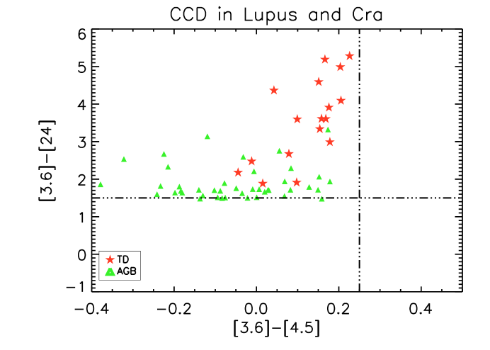
Figure 1: Spitzer color-color diagram for the southern sample. Contaminating AGB stars greatly dominate the sample with [3.6] – [24] $<$ 1.8.

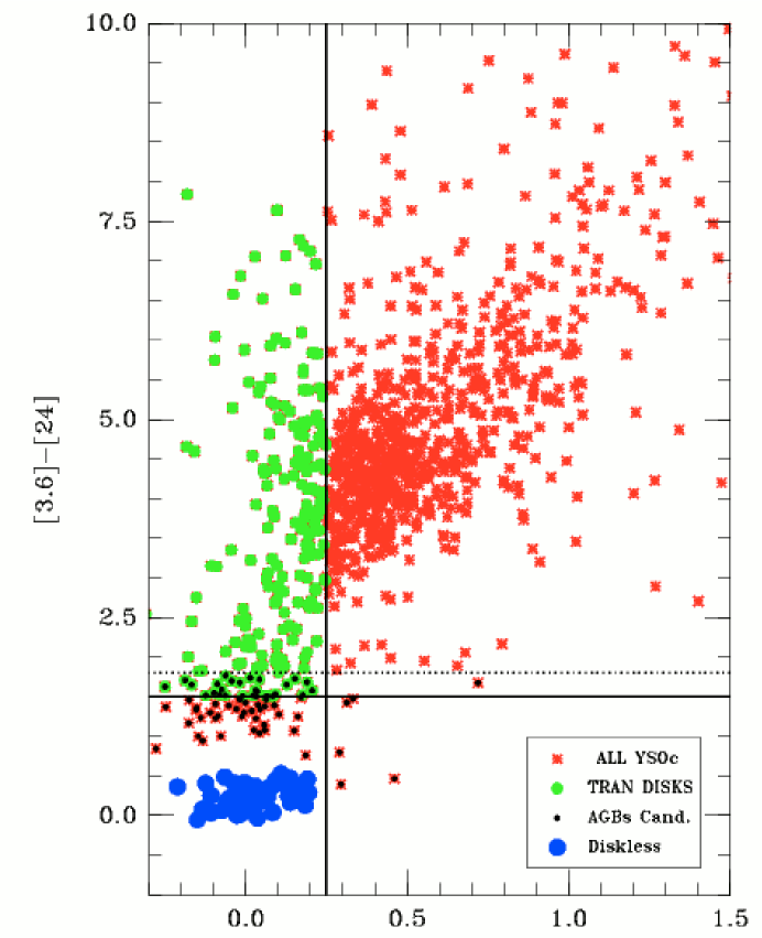
Figure 2: Spitzer c2d systems classified into YSO candidates, AGB candidates, and transition disk candidates according to simple color cuts based on the results of our spectroscopic follow-up program (see text for more details).

The generally large fraction of giant stars in our sample of transition disk candidates allows to investigate possible refinements of our color selection algorithm. Figure 1 shows the color-color diagram of the 60 selected southern transition disk targets of this paper. All transition disk candidates in our sample with $[3.6]-[24]<1.8$ turned out to be giant stars. This agrees quite well with the results obtained for the Ophiuchus sample where 4/6 transition disk candidates with [3.6]-[24] $<$ 1.8 had to be classified as giant stars (see Paper I, Fig. 1). Consequently, one may derive an estimate of the contamination of YSO catalogs due to background giant stars by applying this simple color cut. Figure 2 and 3 show the transition disk candidates and AGB candidates for both the c2d and GB catalogs including all star forming regions. Note, that we here apply color selection criteria only, i.e. the requirements of $R<18$ mag and $K<11$ mag that have been used to define the transition disk candidate sample for our multiwavelength follow-up program are not incorporated. Instead, here we are interested in estimating the fraction of YSO candidates in a given cloud that are likely to be AGB stars based on their very low $24\mu$m excess.

The resulting rough estimates of giant star contamination are given in Table 3 separated by catalog and cloud. According to these estimates, the AGB contamination is expected to vary significantly ranging from $\sim 1-85$ per cent. This shows that AGB contamination can have an important impact on studies that are based on the pure numbers of YSOs as provided by the c2d and GB catalogs. For example, star formation rates as determined e.g. in Heiderman et al. (2010) might become significantly smaller if AGB contamination is taken into account.

Apparently, applying the new more restrictive color selection could also significantly increase the success-rate of identifying YSOs directly from color selection criteria and future follow-up studies may take this into account.

4.3 Characterizing southern transition disks

The Spitzer and alternative names, 2MASS and Spitzer fluxes, and the USNO-B1 R-band magnitudes and the relevant information derived from our follow-up observations for the remaining 17 bona fide transition disk candidates are listed in Tables 4 and 5. In what follows, we use the data discussed in Section 3 to characterize our sample of transition disks.

4.3.1 Spectral types

In oreder to determine the spectral types of the transition disks in our sample we use the equations by Cruz & Reid (2002) that empirically relate the spectral type with the strength of the TiO5 molecular band. The uncertainty of this method is estimated to be $\sim$0.5 subclasses. For most of our transition disk objects, estimates of the spectral types have been provided previously (Hughes et al., 1993, 1994; Krautter et al., 1997; Walter et al., 1997; Sicilia-Aguilar et al., 2008). The spectral types obtained by us and those given in the literature are listed in Table 5 and we find good agreement. All but one system (# 2) have been classified as M-dwarfs. For target # 2, we adopt the spectral type K0 given by Hughes et al. (1993).

4.3.2 Multiplicity

Binarity can play an important role in the context of transition disks as the presence of a close stellar companion may cause the inner hole, i.e. some of the transition disks in our sample might actually be nothing else but circumbinary disks. Some systems in our sample have been previously identified as wide binaries. Merín et al. (2008) carried out an optical survey of the Lupus I, III, IV regions using bands Rc, Ic, ZwI of the Wide-Field Imager (WFI) attached to the ESO 2.2-m telescope at La Silla Observatory. Visual inspection of the images revealed that objects # 1, # 3, # 4, and # 9 are wide binary systems with companions at projected separations of 420, 1000, 600, and 560 AU considering the distance of the Lupus clouds.

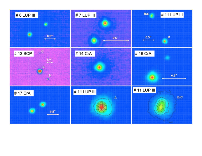
Figure 4: The K_s-band images of the six multiple systems that have been detected with our VLT-AO observations (objects # 6, 7, 11, 13, 16, and 17) and of object # 14, which has been identified as a close binary with a 0.13^′′ separation from speckle observations in 2001 (Köhler et al., 2008). The putative companion in object # 14 remains unresolved by our 2009 observations. Targets # 11 and 13 are triple systems. In the former case, the tighter components are not fully resolved, but their presence can be inferred from the highly elongated image (lower right panel).

We have newly identified six multiple systems by visual inspection of the NaCo images, objects # 6, # 7, # 11, # 13, # 16, and # 17 (see Figure 4). The projected separations are 0.7^′′, 0.4^′′, 1.15^′′, 1.8^′′, 0.5^′′, 0.5^′′ corresponding to 140, 80, 230, 234, 75, 75 AU at the corresponding distances. Object # 13 is a triple system, i.e. a binary with an additional faint companion at 3^′′ (390 AU).

For each binary system, we searched for additional tight companions by comparing each other’s point-spread functions (PSFs). The PSF pairs were virtually identical in all cases, except for target # 11. The south-west component of this target has a perfectly round PSF, while the south-east component, $\sim$1.5^′′ away, is clearly elongated (see Figure 4). Since variations in the PSF shape are not expected within such small angular distances and this behavior is seen in both the J- and K_s-band images, we conclude that target # 11 is likely to be a triple system.

We have also searched in the literature for additional companions in our sample that our VLT observations could have missed. In addition to multiple systems discussed above, we find that # 14 has been reported by Köhler et al. (2008) as a binary system with a projected separation of 0.13^′′ (corresponding to 20 AU) and flux ratio of 0.7 using speckle interferometry at the New Technology Telescope in 2001. We see no evidence for a bright companion in our NaCo images (see Figure 4). However, since our AO images were taken 8 years later than the speckle data, it is possible that the projected separation had changed enough in the intervening years for the binary to become unresolved.

Hence, our sample consists of eleven multiple systems, i.e. nine binaries (objects # 1, 3, 4, 6, 7, 9, 14, 16, 17), and two triples (objects # 11 and 13). Only in the cases of the close B/C pair in object # 11 and # 14 the binary separation is small enough to suspect that the companions might have tidally disrupted the circumbinary disk thereby causing the inner hole inferred from the SED. However, in neither case the circumbinary nature can be confirmed because it is unknown whether the IR excess in object # 11 originates in the wide A component or the close B/C pair and the multiplicity of object # 14 is not confirmed by our observations. We therefore only consider these two objects to be circumbinary disk candidates. Table 5 lists the projected angular separations of the systems.

4.3.3 Disk Masses

Andrews & Williams (2005, 2007) modeled the IR and submillimeter SEDs of circumstellar disks and found a linear relation between the submillimeter flux and the disk mass that has been calibrated by Cieza et al. (2008) who obtained

$$M_{\rm{DISK}}\sim 8.0\times 10^{-2}\leavevmode\nobreak\ [\frac{F_{\nu}(0.86\leavevmode\nobreak\ \rm{mm})}{\rm{mJy}}\times(\frac{d_{1}}{140\leavevmode\nobreak\ \rm{pc}})^{2}]\leavevmode\nobreak\ M_{\rm{JUP}},$$ (1)

where $d_{1}$ is the distance to the target. As described in Paper I, disk masses obtained with the above relation are within a factor of 2 of model derived values, which is certainly good enough for the purposes of our survey. However, one should keep in mind that larger systematic errors can not be ruled out (Andrews & Williams, 2007) as long as strong observational constraints on the grain size distributions and the gas-to-dust ratios are lacking.

Adopting distances of 150 pc to Lupus IV, 200 pc to Lupus III (Comerón, 2008), 130 pc to Scp (Hatchell et al. in preparation), and 150 pc to CrA (Sicilia-Aguilar et al., 2008) we use Equation (1) to estimate disk masses for the 17 systems in our sample (see Table 6). 50$\%$ (i.e. 7/17) of the targets have been detected at 8510 $\mu$m (Table 5). The corresponding disks masses range from $1-9$ M_JUP. Adopting a flux value of 3$\sigma$ for targets with non-detected emission, we derive upper limits for the remaining targets of $\sim\,1-4$ M_JUP. Most of our targets have disk masses $<\leavevmode\nobreak\ 1-2$ M_JUP, but 5 targets have disk masses typical for CTTSs ($\sim$3 – 10 M_JUP). The most massive disks are detected around objects # 2 and # 3, with 9 and 6 M_JUP, respectively.

4.3.4 Accretion rates

The accretion rate is the second crucial parameter necessary to distinguish between the different mechanisms that may form inner opacity holes in circumstellar transitions disks. Most PMS stars show H$\alpha$ emission, either generated from chromospheric activity or magnetospheric accretion (Natta et al., 2004). While non-accreting objects show rather narrow ($<200$ km s^-1) and symmetric line profiles of chromospheric origin, the large-velocity magnetospheric accretion columns produce broad ($>200$ km s^-1) and asymmetric line profiles. As in Paper I we estimate the accretion rates of our transition disk systems according to the empirical relation obtained by Natta et al. (2004), i.e.

$$log(M_{\mathrm{acc}}(M_{\odot}\leavevmode\nobreak\ \rm{yr}^{-1}))=-12.89(\pm 0.3)+9.7(\pm 0.7)\times 10^{-3}\Delta V(\rm{km\leavevmode\nobreak\ s^{-1}})$$ (2)

which is supposed to be relatively well calibrated for velocity widths covering $\Delta\,V=200-600$ km s^-1, which corresponds to accretion rates of $10^{-11}\leavevmode\nobreak\ \rm{M}_{\odot}\leavevmode\nobreak\ \mathrm{yr}^{-1}<\rm{M}_{\rm{acc}}<10^{-7}\leavevmode\nobreak\ \rm{M}_{\odot}\leavevmode\nobreak\ \mathrm{yr}^{-1}$. However, the empirical dividing line between accreting and non-accreting objects has been placed slightly shifted by different authors at $\Delta\,V$ between 200 km s^-1 (Jayawardhana et al., 2003) and 270 km s^-1 (White & Basri, 2003). For systems with $\Delta\,V\sim\,200-300$ km s^-1 we therefore separate accreting and non-accreting objects based on the (a)symmetry of the H$\alpha$ emission line profile and take into account the spectral type because accreting lower mass stars tend to have narrower H$\alpha$ emission lines.

To measure the H$\alpha$ velocity width $\Delta\,V$ we considered for each system the spectral range that corresponds to H$\alpha\pm 2500$ Km/s. The continuum plus emission profile were fitted with a Gaussian plus parabolic profile. The parabolic fit was then used to normalized the spectrum. A single Gaussian profile was sufficient here, being the emission single or double-peaked, as at this stage we were only interested in obtaining a good parabolic fit for the normalization. Once the continuum had been normalized we measured $\Delta\,V$ at 10 per cent of the peak intensity. The obtained velocity dispersion of the H$\alpha$ emission lines and the corresponding accretion rate estimates are given in Table 5 and Table 6, respectively. The obtained accretion rates should be considered order-of-magnitude estimates due to the large uncertainties associated with Equation (2) and the intrinsic variability of accretion in T Tauri stars.

Our sample shows a large diversity of H$\alpha$ signatures. Five targets are classified as non-accreting objects that clearly show symmetric and narrow H$\alpha$ emission line profiles ($<$ 200 km s^-1, see Figure 5) as expected from chromospheric activity. For all these non-accreting objects, we estimate an upper limit of the accretion rate, i.e. $\rm{M}_{\mathrm{acc}}<10^{-11}$ M_⊙ yr^-1.

We classify the remaining 12 transition disk objects as accreting. The majority of them (10) show clearly broad and asymmetric emission-line profiles (see Figure 6). However, targets # 8 and # 12 represent borderline cases with a rather small velocity dispersion for accreting systems ($\Delta\,V\sim 200$  km s^-1) and not clearly asymmetric line profiles. Such borderline systems require a more detailed discussion. Both stars are of late spectral type (M4-M5) and very low-mass stars tend to have narrower H$\alpha$ lines than higher mass objects because of their lower accretion rates (Natta et al., 2004) and their lower gravitational potentials (Muzerolle et al., 2003). Object # 12 additionally shows $8\,\mu$m excess emission indicating the presence of an inner disk. Given all the available data, we classify targets # 8 and # 12 as accreting objects, but warn the reader that their accreting nature is less certain than that of the rest of the objects classified as CTTSs. As accretion in T Tauri stars can well be episodic, mutli-epoch spectroscopy would be useful to unambiguously identify the accreting nature of these two systems.

The mass accretion rates estimated for the 12 disks classified as accreting systems range from 10^-11 M_⊙ yr^-1 to 10^-7.7 M_⊙ yr^-1

5 Discussion

5.1 The origin of the inner opacity hole

With the collected information presented in the previous sections we have at hand the following information of the Spitzer-selected transition disks in our sample:

• Detailed SEDs that we quantify with the two-parameter scheme introduced by Cieza et al. (2007), which is based on the longest wavelength at which the observed flux is dominated by the stellar photosphere, $\lambda_{\mathrm{turn−off}}$, and the slope of the IR excess, $\alpha_{\mathrm{excess}}$, computed as $d\log(F_{\lambda})/d\log(\lambda)$ between $\lambda_{\mathrm{turn−off}}$ and $24$ $\mu$m.

• Multiplicity information from the literature and AO IR imaging.

• Disk mass estimates based on measured submillimeter flux.

• Accretion rate estimates derived from H$\alpha$ line profiles.

This information allows to separate the sample according to the physical processes that are the most likely cause of the inner opacity hole: grain growth, planet formation, photoevaporation, or close binary interactions. In what follows we briefly review each process that might be responsible for the formation of the inner opacity holes, describe our criteria for classifying transition disks, and discuss the corresponding sub-samples of transition disks obtained.

5.2 Accreting transition disks

The presence of accretion in classical transition disk objects raises the question how the inner disk can be cleared of small grains while gas remains in the dust hole. The two mechanisms that can explain the coexistence of accretion and inner opacity holes are grain growth and dynamical interactions with (sub)stellar companions.

5.2.1 Grain growth

Due to both, the higher densities and the faster relative velocities of particles in the inner parts of the disk, this disk region offers much better conditions for dust agglomeration than the outer parts of the disk. Therefore, significant grain growth should start in the inner disk regions. As soon as the grains grow to sizes exceeding the considered wavelength ($r>>\lambda$), the opacity decreases until an inner opacity hole forms. Early models by Dullemond & Dominik (2005) taking into account only dust coagulation predict much too short timescales of the order of $10^{5}$ yrs to clear the entire disk of small grains, which is inconsistent with observed SEDs of most classical T Tauri stars. A more reliable picture combines coagulation and collisional fragmentation or erosion of large dust aggregates (Dominik & Dullemond, 2008).

As a gradual transition between the inner and outer disk is predicted by grain growth and dust settling models (dullemond+dominik08-1; Weidenschilling, 2008), grain growth dominated disks should have $\alpha_{\mathrm{excess}}\leq\,0$ (i.e., falling mid-IR SEDs) while $\lambda_{\mathrm{turnoff}}$, associated with the size of the hole, can differ over a rather wide range of values. Although grain growth does not directly affect the gas, it may increase accretion because the inner opacity hole can lead to efficient ionization and trigger the MRI instability (Chiang & Murray-Clay, 2007).

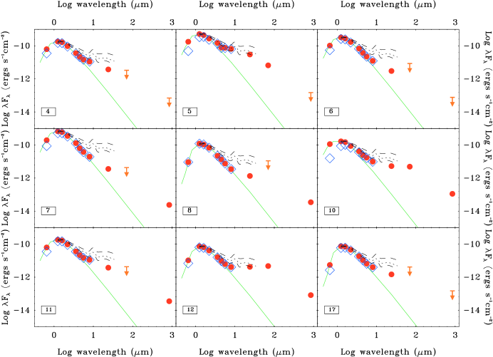
Figure 7: SEDs of the 9 grain growth candidates. Disk masses range from $<$ 1.1 to 5.1 M_JUP, and accretion rates from $10^{-11}$ to $10^{-9.3}$ M_⊙ yr^-1. The filled circles are detections, while the arrows represent 3$\sigma$ limits. The open squares correspond to the observed optical and near-IR fluxes before being corrected for extinction as in Paper I. For each object, the average of the two R-band magnitudes (from the USNO-B1 catalog) listed in Table 4 has been used. The classification of object # 5 and 10 as grain growth dominated is slightly uncertain as classical T Tauris stars of late M-types can have similar SEDs (Ercolano et al., 2009). The solid line represents the stellar photosphere normalized to the extinction-corrected J band. The dotted lines correspond to the median mid-IR SED of CTTSs calculated by Furlan et al. (2006). The dashed lines are the quartiles.

Among the 17 transition disks in our sample, nine objects are accreting and are associated with $\alpha_{\mathrm{excess}}$ $\leq\,0$. The corresponding SEDs are shown in Figure 7. The grain growth candidate systems in our sample could be confounded with accreting classical T Tauri M-stars as predicted by Ercolano et al. (2009). However, most of our grain growth dominated disks have SEDs close to the stellar photosphere up to $\sim 8-10\,\mu$m and we therefore do not expect significant contamination by non transition disks. The only exceptions being objects # 5 and 10 with a small value of $\lambda_{\mathrm{turn−off}}$$=2.2$ and to some extend # 4 and # 11 ($\lambda_{\mathrm{turn−off}}$$=4.5$). We recommend the reader to keep in mind the uncertain classification of these four systems.

Compared with the Oph sample (Paper I) the accretion rates obtained for grain growth dominated disks are slightly smaller (i. e. $10^{-9.3}-10^{-11}$M_⊙ yr^-1). This might be related to the slightly lower stellar masses or to advanced viscous evolution as discussed in D’Alessio et al. (2006).

The grain growth dominated disks are located in the Lupus  III, IV (8) and the CrA (1) star-forming regions.

5.2.2 Dynamical interactions with (sub)stellar companions

The truncation of the disk as the result of dynamical interactions with companions was first proposed by Lin & Papaloizou (1979). More recently, it has been shown that most PMS stars are in multiple systems with a lognormal semi-major axis distribution centered at $\sim\,30$ AU (e.g., Ratzka et al., 2005). A significant fraction of the binaries in the star-forming regions considered here should therefore be tight binaries with separations of $1-20$ AU. Disks in such close binary system will be tidally truncated at $\sim\,2\leavevmode\nobreak\ \times$ the binary separation and a circumbinary disk with an inner hole is formed (Artymowicz & Lubow, 1994). The corresponding SED is that of a transition disk. However, the circumbinary nature does not exclude additional evolutionary processes to be at work and we therefore provide an additional classification based on the disk properties only (see Table 6).

Identification of companions that may cause the formation of a circumbinary disk is possible either due to high-resolution imaging or by measuring radial velocity variations. As described in Sect. 3.2, we identified 2 circumbinary disk candidates among our 17 transition disk systems. One of them, object # 11 was discovered by inspecting the NaCo images obtained with the VLT, while the close binary nature of object # 14 has been discovered by Köhler et al. (2008) using speckle interferometry at the NTT.

Object # 11 shows signs of strong accretion and has a SED with $\alpha_{\mathrm{excess}}\sim-1$ in agreement with grain growth. It is currently not clear under which conditions gap-crossing streams can exist and allow accretion onto the central star to proceed, but signs of accretion in circumbinary systems (Carr et al., 2001; Espaillat et al., 2007) indicate that accretion is likely to continue. On the other hand, object # 14 is a non-accreting system such as the known binary CoKu Tau$/$4 (Ireland & Kraus, 2008). According to its L_DISK/L_∗ ratio we classify this system as a circumbinary/photoevaporation disk candidate.

As a final note of caution, we would like to stress that both objects discussed above (# 11 and # 14) are circumbinary disk candidates. As all but one of our targets are M-type stars, most companions potentially responsible for their transition disk SEDs are expected to lie at closer separations than those probed by the AO images. Therefore, our sample of circumbinary disk candidates is incomplete and heavily biased towards large separations. Methods more sensitive to closer companions such as aperture masking and/or radial velocity observations are required to draw firm conclusions on circumbinary disk fractions.

5.2.3 Giant Planet formation

The most exciting way to produce a transition disk SED is by giant planet formation. According to early models as well as recent numerical simulations, the formation of giant planets involves the formation of gaps and holes in the circumstellar disk (Lin & Papaloizou, 1979; Artymowicz & Lubow, 1994).

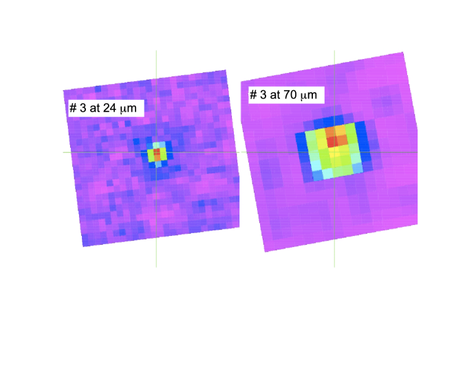
Figure 8: The 24 and 70 $\mu$m images of object # 3. We find no evidence for extended emission from the molecular cloud. In both mosaics, the detections are consistent with a point source at the location of the target (marked by the crosshairs). See the electronic edition of the Journal for a color version of this figure.

As in the case of (sub)stellar companions it is uncertain if and to what extent accretion proceeds in the presence of a forming giant planet. Therefore, the most important sign of ongoing planet formation remains a sharp inner hole, usually corresponding to $\alpha_{\mathrm{excess}}$$>0$ (i.e., a rising mid-IR SED). However, although very useful, the definition of $\alpha_{\mathrm{excess}}$ is incomplete, as the SED may also steeply rise at wavelengths longer than $24\,\mu$m. A spectacular example illustrating this is given by object # 3. While  $\alpha_{\mathrm{excess}}$$\sim\,-2.2$, the SED steeply rises between $24\,\mu$m and $70\,\mu$m. Furthermore, object # 3 shows clear signs of accretion ($M_{\mathrm{acc}}=\leavevmode\nobreak\ 10^{-10.1}$ M_⊙/yr) and of harboring a relatively massive disk (M_DISK$\leavevmode\nobreak\ \sim 6$ M_JUP). Since this is a very atypical object, we verified that the large 70 $\mu$m flux is not contaminated by extended emission from the molecular cloud. We examined the 24 and 70$\mu$m mosaics and verified that the detections are consistent with point sources at the source location (see Figure 8). A more typical transition disk system that might represent a currently planet forming disk is target # 15 with a clearly positive value of $\alpha_{\mathrm{excess}}$ and a high accretion rate. A borderline case between grain growth and planet forming disks is object # 2. A high accretion rate combined with $\alpha_{\mathrm{excess}}$$\sim 0$ could be consistent with both scenarios. Keeping in mind the ambiguity, we classify object # 2 as a planet forming disk candidate because it could potentially be an extremely interesting object. The SED of object # 2 might be explained by a discontinuity in the grain size distribution rather than an inner opacity hole. While the inner part of the disk still contains small grains, outer regions of the disk might be dominated by slightly larger dust particles. Such a scenario is in excellent agreement with the predictions of numerical simulations performed by Rice et al. (2006). They show that the planet–disk interaction at the outer edge of the gap cleared by a planet can act as a filter passed by small particles only which produces a discontinuity in the dust particle size. To firmly establish its nature object # 2 deserves further follow-up observations (e.g., high resolution imaging with ALMA).

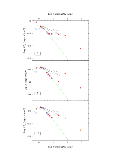
Figure 9: SEDs of the three planet forming candidates. While object # 15 can be considered a classical planet forming candidate system with $\alpha_{\mathrm{excess}}$ $>0$ and $\lambda_{\mathrm{turn−off}}$ = 8.0 $\mu$m, the other two systems are somewhat peculiar: target # 3 shows a very steep rise in flux observed at 70 $\mu$m, which indicates a very large inner hole and object # 2 being relatively close to a full disk but with signs for a small and sharp inner hole. Disk masses are 9.1, 5.6 and $<$ 2 M_JUP for objects # 2, # 3, and # 15; respectively. The solid line as well as the dashes and dotted lines are the same as in Fig. 7.

The SEDs of the three candidates for ongoing giant planet formation in our sample are shown in Figure 9. The hosting forming giant planets candidates are located in the Lupus III, IV (2) and the CrA (1) star-forming regions.

5.3 Non-accreting objects

The second main class of transition disks are those that do not show signs of accretion. In such disks the inner opacity hole, i.e. the lack of small dust particles in the inner disk regions, is likely to coincide with a gas hole, i.e. the inner disk is completely drained.

5.3.1 Photoevaporating disk

The most important process for clearing the inner disk in transitions disks that do not accrete is photoevaporation (e.g. Alexander et al., 2006). According to this model, extreme-ultraviolet (EUV) photons, originating in the stellar chromosphere, ionize and heat the circumstellar hydrogen which is then partly lost in a wind. This process is supposed to work in all circumstellar disks but becomes important only when the accretion rate drops to values similar to the photoevaporation rate. Then, the inner disk drains on the viscous timescale supported by the generation of the MRI (Chiang & Murray-Clay, 2007). Once an inner hole has formed, the inner disk rim is efficiently radiated and the entire disk should therefore quickly disappear. Photoevaporating disks should have negligible accretion (Williams & Cieza, 2011). To separate photoevaporating disks from debris disks, we require the disk luminosity to be higher than that seen in the brightest bona-fide debris disks, i.e. L_DISK/L_∗ $\geq\,10^{-3}$ (Bryden et al., 2006; Wyatt, 2008). We thus obtained $70\leavevmode\nobreak\ \mu$m upper limits from the noise of the $70\leavevmode\nobreak\ \mu$m Spitzer mosaics at the source location and calculated L_DISK/L_∗ for our sample by integrating the stellar fluxes and disk fluxes over frequency (see Section 5.1.3 in Paper I for details of the $70\leavevmode\nobreak\ \mu$m data analysis and the L_DISK/L_∗ calculation).

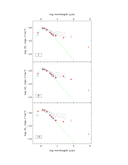
Figure 10: SEDs of the 3 transition disks classified as photoevaporating disk candidates. The symbols, solid line as well as the dashes and dotted lines are the same as in Figure 7. None of these systems have been detected at submillimeter wavelength and consequently only upper limits for the disk masses could be derived. We conclude that photoevaporation seems to be less efficient than has recently been suggested.

We classify three transition disks as photoevaporating disk candidates with negligible accretion (M_acc $<$ 10^-11 yr^-1) but L_DISK/L_∗ $\geq\,10^{-3}$ (Table 6). According to our submillimeter measurements, all these three systems have small disk masses ($<1-3.4$ M_JUP, Table 6). In fact, for all photoevaporation candidates we could only derive upper limits on the disk mass. The SEDs of the three systems classified as photoevaporating disk objects are shown in Figure 10. The photoevaporated disks are located in the Lupus III, IV (2) and CrA (1) star-forming regions.

5.3.2 Debris disk

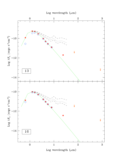
Figure 11: SEDs of the 2 debris disk candidates identified in our sample. We distinguish between debris disks and photoevaporation applying an ad-hoc limit on L_DISK/L_∗ $\stackrel{{\scriptstyle<}}{{\scriptstyle\sim}}$ 10^-3. The detection of the gas component in photoevaporating disks (e.g. with ALMA) may lead to a more physically motivated separation between the two sub-samples. The solid line as well as the dashes and dotted lines are the same as in Figure 7.

Photoevaporation can be considered as a transition stage between primordial and debris disks. Debris disks contain a small amount of dust and are gas-poor. We find two debris disk candidates, i.e. non-accreting systems with L_DISK/L_∗$<\,10^{-3}$, among our 17 transition disks (see Figure 11). The debris disks are located in the CrA (1) and Scp (1) star-forming regions.

5.4 Implications for disk evolution

5.4.1 Heterogeneity of transition disks

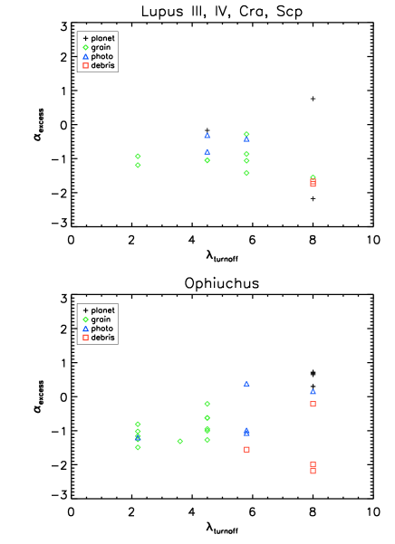
Figure 12: $\alpha_{\mathrm{excess}}$ vs $\lambda_{\mathrm{turn−off}}$ for transition disks identified in Paper I and the present work. The locations of the Ophiuchus transition disk sample from this work (top panel) and Paper I (bottom panel) cover very similar ranges in the $\alpha_{\mathrm{excess}}$  versus $\lambda_{\mathrm{turn−off}}$ plane. Different symbols indicate different formation processes of the inner opacity hole. In general, the Lupus, Cra, and Scp data confirm our previous findings: planet forming disks have large values of $\alpha_{\mathrm{excess}}$  and $\lambda_{\mathrm{turn−off}}$, grain growth dominated disks should have small $\alpha_{\mathrm{excess}}$ , but cover the entire range of $\lambda_{\mathrm{turn−off}}$; and debris disks have extremely low values of $\alpha_{\mathrm{excess}}$  and the IR excess starts at long $\lambda_{\mathrm{turn−off}}$. However, two systems clearly show that $\alpha_{\mathrm{excess}}$ and $\lambda_{\mathrm{turn−off}}$ alone cannot fully characterize transition disks. We identified one planet forming disk candidate with $\alpha_{\mathrm{excess}}$$<0$ but indications of a sharp hole at longer wavelength (object # 3) and one planet forming candidate with $\lambda_{\mathrm{turn−off}}$ = 4.5 $\mu$m (object # 2) have been found.

In the previous sections, we presented detailed follow-up observations of 60 Spitzer-selected transition disk candidates located in the southern star-forming regions Lupus I, III, IV, V, VI, CrA, and Scp. Optical spectroscopy revealed that only 17 systems of these candidates are genuine transition disk T Tauri stars. Deriving estimates for the accretion rates, disk masses, and multiplicity of these 17 systems we classified them as dominated by grain growth (9), giant planet formation (3), photoevaporation (3), or being in the final debris disk stage (2). Two of these transition objects, one grain growth (# 11) and one photoevaporating (# 14), are circumbinary disk candidates, which offers the possibility of tidal truncation as mechanism responsible for an inner hole in the common/shared disk. Combining these results with those presented in Paper I, we now have at hand well-defined and well characterized samples of transition disks from several different star-forming regions. Figure 12 summarizes the properties of these samples based on $\alpha_{\mathrm{excess}}$ and $\lambda_{\mathrm{turn−off}}$. The main aim of these series of papers is to progress with our understanding of circumstellar disk evolution and to compare transition disk samples of different clouds is key in this respect. Table 7 shows the fractions of different types of transition disks for Ophiuchus (age $\approx$ $0.3-2.1$ Myr, Wilking et al. 2005, and references therein), CrA (age $\approx$ 1 Myr, Sicilia-Aguilar et al. 2008), and Lupus I, III, IV (age $1.5-4$ Myr, Merín et al. 2008). All YSO candidates followed up spectroscopically located in Lupus V, VI turned out to be AGB stars. These clouds have been recently estimated to be a few Myrs older (Spezzi et al., 2011) based on the dominance of Class III systems. As we have shown in Section 4.1, at least $\sim 50$ % of the claimed class III systems located in Lupus V, VI are very likely to be AGB stars. This reduces the fraction of class III objects to values similar to those obtained for Lupus III. Based on this, Lupus V, VI, and III could well be of a very similar age.

The main result that can be obtained from Table 7 clearly is that young clouds ($\raisebox{-1.72218pt}{$\stackrel{{\scriptstyle<}}{{\scriptstyle\sim}}$}\ 1-4$ Myr) contain a mixture of grain growth, photoevaporating, debris, and tidally disrupted transition disks. It is clear that all states of disk evolution are already present at this age range, which implies that different disks evolve at different rates and/or through different evolutionary paths. An important difficulty in constraining disk evolution is that stellar ages obtained from isochrones are very uncertain for individual systems. An analysis of the stellar age distributions of each disk category is therefore postponed to paper III (Cieza et al. 2012, ApJ submitted), where we discuss a larger sample of well characterized transition disk objects including the systems presented here.

5.4.2 Evidence for low photoevaporation rates

The general picture of photoevaporation is the following. In very young disks, the accretion rate largely exceeds the evaporation rate and the disk evolves virtually unaffected by photoevaporation. As the accretion rate is decreasing with time, the disk necessarily reaches the time when the accretion rate equals the photoevaporation rate and the outer disk is no longer able to resupply the inner disk with material. At this point, the inner disk drains on the viscous timescale ($\stackrel{{\scriptstyle<}}{{\scriptstyle\sim}}$ $10^{5}$  yr) and an inner hole of a few AU in radius is formed in the disk. The inner disk edge is now directly exposed to the EUV radiation and the disk rapidly photoevaporates from the inside out.

Early models of EUV photoevaporation predict evaporation rates of $10^{-10}-10^{-9}$ M_⊙/yr (Hollenbach et al., 1994). More recent simulations taking into account X-ray (Owen et al., 2010) and/or far-ultraviolet (FUV) irradiation (Gorti & Hollenbach, 2009) in addition to the EUV photons, largely exceed these early predictions, reaching photoevaporation rates of the order of $10^{-8}$ M_⊙/yr (see also Armitage, 2011).

As in steady state accretion disks the mass transfer through the disk is roughly proportional to the mass accretion rate onto the star, a crucial prediction of the photoevaporation model is that high photoevaporation rates imply high disk masses at the time the inner disk is drained. In particular, models with efficient X-ray photoevaporation predict a significant population of relatively massive ($\sim$7 M_JUP) non-accreting transition disks (Owen et al., 2011).

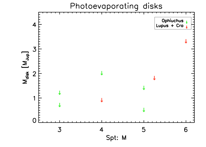
Figure 13: The masses of the photoevaporating disk candidates in our sample. Clearly, massive photoevaporating disks predicted by high evaporation rates are absent.

Figure 13 shows the upper limits (derived from submillimeter non detections) on the disk masses of the photoevaporating transition disks in all the clouds we considered so far. Even taking into account uncertainties in our classification of photoevaporation candidates, it is evident that large numbers of non-accreting but massive disks do not exist. This indicates that photoevaporation is less efficient than predicted by the models described above. However, one has to take into account that the sample of transition disks considered here contains low-mass stars only while model calculations have been performed exclusively for more massive stars $\sim 1$M_⊙. Therefore, either a more homogeneous sample of photoevaporating disk systems covering a larger range of host star masses (earlier spectral types) or simulations of photoevaporation for disks around low-mass stars are required to provide a final answer on this issue.

5.5 Current limitations and future perspectives

Of course, our classification of transition disk objects is based on rather rough empirical relations and requires to carefully consider possible caveats. An obvious uncertainty concerns our multiplicity survey. The method of direct detection of companions is obviously more sensitive to binaries with large separations and low inclinations. Our NaCo observations are sensitive to projected separations of $\sim 10-15$ AU given the distance to our targets and – depending on the intrinsic distribution of orbital separations – we may therefore miss a significant fraction of close binaries. To overcome this observational bias we are currently performing radial velocity measurements of our targets using VLT/UVES. The method of detecting radial velocity variations is more sensitive to small separations and high inclinations and therefore complements the imaging results presented here. We will present the results in a forthcoming paper. However, the fact that only 6 of the 43 transition disks studied herein and in Paper I are circumbinary disk candidates strongly suggests that binaries at the peak of their separation distribution ($\sim$ 30 AU) do not result in transition disk objects as such stellar binaries would be easily detectable by our AO observations. Instead, they are likely to destroy the disk rather quickly (Cieza et al., 2009).

Another uncertainty in our classification procedure is the rather ad-hoc separation between photoevaporating and debris disk systems by using a limit in L_DISK/L_∗. However, there is a physical and not only phenomenological difference between these two types of transition disks. Photoevaporating disks are dissipating primordial disks and should have gas rich outer disks while the debris disks should be gas poor. Molecular line observations with the Atacama Large Millimeter/Submillimeter Array (ALMA) of non-accreting disks will be able to distinguish between the two types of objects.

A huge problem related to the process of photoevaporation is that the mass loss rates predicted by different models differ by up-to two orders of magnitude (see e.g. Williams & Cieza, 2011). The disk mass at the time photoevaporation opens a hole in the disk is directly connected to the photoevaporation rates. Measuring the disk masses of photoevaporating disks could therefore significantly constrain theoretical models of photoevaporation. However, all of the photoevaporting disk candidates remain undetected and we can only put upper limits to their masses. Fortunately, ALMA will be much more sensitive than all presently available telescopes and will soon be able to measure the masses of many bona fide photoevaporating disks. ALMA should also be able to measure, through high resolution continuum observations at multiple wavelengths, the radial dependence in the grain size distribution expected in the grain-growth dominated disks.

Finally, the recent identification using the aperture masking technique of what seems to be forming planets within the inner cavities of the transition disks around T Cha (Huélamo et al., 2011) and LkCa 15 (Kraus & Ireland, 2012) strongly encourages to obtain similar observations for the three planet-forming disk candidates identified herein, objects # 2, # 3, and # 15. Any system with a planet still embedded in a primordial disk would represent an invaluable laboratory to study planet formation with current and future instrumentation.

6 Summary

We have carried out a multifrequency study of Spitzer-selected YSO transition disk candidates located in the Lupus complex (53), CrA (5), and Scp (2). We obtained submillimeter observations (APEX), optical high resolution echelle spectroscopy (Clay/Mike, Du Pont/echelle), and NIR images (from AO imaging VLT/NaCo). After deriving spectral types of each target, 43 AGB stars were removed (Lupus complex (41), CrA (1), and Scp (1)), leaving a sample of 17 genuine transition disk systems. We find that the vast majority of AGB stars have [3.6]-[24] $<$ 1.8, underscoring the need for a spectroscopic confirmation of YSO candidates with small 24$\mu$m excesses. The data obtained for the 17 transition systems allows to estimate multiplicity, stellar accretion rates, and disk masses thereby allowing to identify the physical mechanism that is most likely to be responsible for the formation of the inner opacity hole. The observational results of this study can be summarized as follows:

1. The derived spectral classification indicates that all but one (object # 2, K0) central star are M-type stars, in agreement with previous results (Comerón, 2008).

2. 12/17 targets are accreting objects (i.e. asymmetric H$\alpha$ profile having a velocity width $\stackrel{{\scriptstyle>}}{{\scriptstyle\sim}}$ 200 km s^-1 at 10$\%$ of peak intensity).

3. $\sim$ 50$\%$ of the sample are multiple systems and among them, two triple systems. Two binary systems have small projected separations and are therefore candidates to host a circumbinary disk.

4. 7/17 targets have flux detection in the submillimeter. For the remaining systems, we derive and upper limit of the disk mass (corresponding to a flux of 3 $\times$ rms). The estimated disk masses for the detected objects cover the range 2 M_JUP–10 M_JUP.

Combining the derived estimates of disk masses, accretion rates and multiplicity with the SED morphology and fractional disk luminosity (L_DISK/L_∗) allows to classify the disks as strong candidates for the following categories:

• 9/17 grain growth-dominated disks (accreting objects with negative SED slopes in the mid-IR, $\alpha_{\mathrm{excess}}$$<$ 0).

• 3/17 photoevaporating disks (non-accreting objects with disk mass $<$ 3 M_JUP, but L_DISK/L_∗$>$ 10^-3).

• 2/17 debris disks (non-accreting objects with disk mass $<$ 2.1 M_JUP and L_DISK/L_∗$<$ 10^-3).

• 2/17 circumbinary disks (a binary tight enough to accommodate both components within the inner hole).

• 3/17 giant planet forming disk (accreting systems with SEDs indicating sharp inner holes).

Inspecting in more detail the different sub-clouds analyzed in this study we find the same heterogeneity of the transition disk population in Lupus III, IV, CrA as in our previous analysis of transition disks in Ophiuchus (Cieza et al., 2010, Paper I). We therefore conclude that photoevaporation, giant planet formation, and grain growth produce inner holes on similar timescales. Not a single transition disks has been found in Lupus I, V, VI. All 33 candidates that have been spectroscopically followed up turned out to be AGB stars which questions the recent interpretation of Spezzi et al. (2011) that Lupus I, V, VI might be relatively old star forming regions dominated by Class III objects.

In addition, our detailed observational analysis of transition disks provides clear constraints on theoretical models of disk photoevaporation by the central star. According to the large evaporation rates predicted by recent models (i.e. see Armitage, 2011), large numbers of massive photoevaporating transition disks systems should exist. In contrast to this prediction, all photoevaporating disk candidates identified in this work and Paper I contain very little mass, indicating much smaller evaporation rates at least for the low-mass stars considered here. Similarly, the low incidence of circumbinary transition disk candidates ($\sim$ 10$\%$) supports the idea that most disks are destroyed rather quickly by companions at $\sim 10-40$ AU separations.

Finally, we emphasize that the 43 transition disk systems discussed in this work and in Paper I represent the currently largest and most homogeneous sample of well-characterized transition disks. Further investigating these systems with new observing capabilities such as ALMA therefore holds the potential to significantly improvement our understanding of the physical processes driving circumstellar disk evolution.

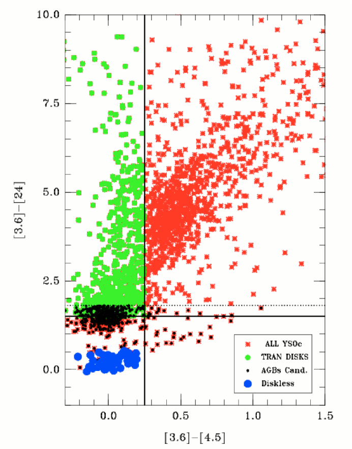
Figure 3: Same as Fig. 2 but for the GB catalog.

Figure 5: Normalized average H$\alpha$ profiles for non-accreting objects with clear H$\alpha$ emission. The horizontal dashed line indicates the 10% peak intensity, where $\Delta$V is measured. The velocity widths are $<$ 200 km s^-1 and the line profiles are symmetric.

Figure 6: Normalized H$\alpha$ profiles of the 12 accreting objects. These systems are considered accreting because either the velocity width is $>$ 200 km s^-1 or the line profile is asymmetric. Note that objects # 8 and 12 represent borderline systems as the $\Delta$V$\sim 200$km/s and the line is not clearly asymmetric (see text for more details).

Table 1: Spectroscopically identified AGB stars

#	Ra (J2000)	Dec (J2000)	Spitzer ID	R	J	H	KS	F3.6	F4.5	F5.8	F8.0	F24	Region	References
	(deg)	(deg)		(mag)	(mJy)	(mJy)	(mJy)	(mJy)	(mJy)	(mJy)	(mJy)	(mJy)
1	234.51292	-33.23269	SSTc2d_J153803.1-331358	13.35	3.91e+02	6.91e+02	6.83e+02	3.47e+02	2.20e+02	1.82e+02	1.26e+02	3.56e+01	Lup I	1
2	235.64750	-34.37292	SSTc2d_J154235.4-342223	14.17	5.16e+02	8.86e+02	8.43e+02	4.00e+02	2.66e+02	2.03e+02	1.40e+02	4.96e+01	Lup I
3	239.93868	-41.91590	SSTc2d_J155945.3-415457	13.18	3.64e+02	7.92e+02	8.86e+02	5.78e+02	3.35e+02	3.23e+02	3.80e+02	2.68e+02	Lup IV	1
4	240.37369	-42.13432	SSTc2d_J160129.7-420804	15.74	7.74e+01	1.57e+02	1.60e+02	9.11e+01	5.86e+01	4.89e+01	3.80e+01	1.79e+01	Lup IV	1
5	240.62463	-41.85307	SSTc2d_J160229.9-415111	17.91	3.95e+01	8.07e+01	8.73e+01	4.99e+01	3.01e+01	2.55e+01	1.82e+01	5.15e+00	Lup IV	1
6	242.19953	-38.83361	SSTc2d_J160847.9-385001	13.71	1.12e+03	1.93e+03	1.89e+03	9.86e+02	4.50e+02	4.37e+02	3.14e+02	1.41e+02	Lup III
7	242.39212	-39.22835	SSTc2d_J160934.1-391342	15.11	5.36e+02	1.20e+03	1.43e+03	5.33e+02	3.99e+02	4.66e+02	2.83e+02	5.35e+01	Lup III	1
8	242.50045	-38.90031	SSTc2d_J161000.1-385401	17.47	2.25e+02	4.13e+02	5.55e+02	3.66e+02	1.76e+02	2.68e+02	2.06e+02	9.72e+01	Lup III	1
9	242.85827	-39.18979	SSTc2d_J161126.0-391123	16.29	6.96e+02	1.43e+03	1.71e+03	1.01e+03	5.99e+02	5.56e+02	3.62e+02	1.05e+02	Lup III	1
10	243.21550	-38.70443	SSTc2d_J161251.7-384216	14.06	5.97e+02	1.04e+03	1.07e+03	6.37e+02	3.49e+02	3.06e+02	2.02e+02	7.43e+01	Lup III	1
11	244.92350	-37.78246	SSTGBS_J16194163-3746568	16.36	6.48e+01	1.27e+02	1.33e+02	8.56e+01	5.64e+01	4.77e+01	3.26e+01	1.02e+01	Lup V	2
12	245.00856	-41.62400	SSTGBS_J16200205-4137264	15.37	6.17e+02	1.24e+03	1.35e+03	7.27e+02	4.28e+02	3.60e+02	2.31e+02	9.00e+01	Lup VI	2
13	245.03960	-41.43343	SSTGBS_J16200950-4126003	15.78	7.69e+02	1.77e+03	2.05e+03	1.40e+03	8.77e+02	7.88e+02	5.20e+02	1.61e+02	Lup VI	2
14	245.13167	-37.51133	SSTGBS_J16203160-3730407	16.96	1.40e+03	2.78e+03	3.38e+03	2.07e+03	1.24e+03	1.27e+03	9.10e+02	2.11e+02	Lup V	2
15	245.22704	-36.91195	SSTGBS_J16205449-3654430	16.03	1.89e+02	3.86e+02	4.12e+02	2.24e+02	1.16e+02	9.97e+01	6.43e+01	2.51e+01	Lup V	2
16	245.35836	-37.51710	SSTGBS_J16212600-3731015	16.69	1.62e+02	4.21e+02	6.41e+02	7.57e+02	5.29e+02	5.18e+02	3.87e+02	1.61e+02	Lup V	2
17	245.37467	-37.03926	SSTGBS_J16212991-3702213	14.84	1.68e+02	3.15e+02	3.31e+02	1.89e+02	9.94e+01	8.37e+01	5.79e+01	5.69e+01	Lup V	2
18	245.41990	-41.37274	SSTGBS_J16214077-4122218	15.98	1.26e+02	2.51e+02	2.64e+02	1.58e+02	8.63e+01	7.36e+01	4.86e+01	1.92e+01	Lup VI	2
19	245.45722	-41.11716	SSTGBS_J16214973-4107017	15.35	1.20e+0	2.30e+02	2.65e+02	1.92e+02	1.34e+02	1.08e+02	7.48e+01	2.40e+01	Lup VI	2
20	245.48435	-37.22131	SSTGBS_J16215624-3713167	17.18	1.95e+0	3.89e+02	4.34e+02	2.43e+02	1.31e+02	1.15e+02	7.38e+01	2.84e+01	Lup V	2
21	245.50680	-37.27693	SSTGBS_J16220163-3716369	16.20	5.48e+0	1.06e+02	1.09e+02	6.50e+01	4.23e+01	3.53e+01	2.48e+01	8.24e+00	Lup V	2
22	245.57457	-36.97127	SSTGBS_J16221789-3658165	16.80	2.68e+02	5.24e+02	5.83e+02	3.42e+02	1.95e+02	1.68e+02	1.08e+02	3.44e+01	Lup V	2
23	245.63924	-41.05499	SSTGBS_J16223341-4103179	16.34	5.72e+02	1.32e+03	1.50e+03	8.22e+02	4.95e+02	4.26e+02	2.87e+02	1.21e+02	Lup VI	2
24	245.67774	-37.35645	SSTGBS_J16224265-3721232	16.08	1.97e+02	4.34e+02	4.97e+02	3.61e+02	2.74e+02	2.47e+02	2.61e+02	1.98e+02	Lup V	2
25	245.76534	-37.49477	SSTGBS_J16230368-3729411	16.02	6.05e+01	1.18e+02	1.20e+02	6.64e+01	4.17e+01	3.55e+01	3.12e+01	1.86e+01	Lup V	2
26	245.79592	-41.28620	SSTGBS_J16231101-4117103	16.48	1.14e+02	2.64e+02	3.00e+02	1.67e+02	1.15e+02	9.21e+01	6.16e+01	1.79e+01	Lup VI	2
27	245.81152	-40.28753	SSTGBS_J16231476-4017151	16.96	1.69e+02	3.56e+02	4.07e+02	2.20e+02	1.36e+02	1.15e+02	8.15e+01	2.86e+01	Lup VI	2
28	245.81661	-41.06693	SSTGBS_J16231598-4104009	13.11	1.97e+03	4.16e+03	4.86e+03	1.80e+03	1.31e+03	1.12e+03	7.36e+02	2.41e+02	Lup VI	2
29	245.85994	-37.86896	SSTGBS_J16232638-3752082	17.31	1.20e+02	2.35e+02	2.99e+02	3.24e+02	2.47e+02	2.33e+02	1.74e+02	4.96e+01	Lup V	2
30	245.88526	-37.87672	SSTGBS_J16233246-3752361	15.74	4.72e+02	9.78e+02	1.06e+03	5.68e+02	3.23e+02	2.85e+02	1.92e+02	7.09e+01	Lup V	2
31	245.91108	-37.52745	SSTGBS_J16233865-3731388	15.80	1.27e+02	2.39e+02	2.53e+02	1.43e+02	7.59e+01	7.05e+01	5.16e+01	3.14e+01	Lup V	2
32	245.95431	-40.43823	SSTGBS_J16234903-4026176	17.12	9.57e+01	2.08e+02	2.33e+02	1.64e+02	1.13e+02	9.72e+01	7.79e+01	2.52e+01	Lup VI	2
33	245.99615	-37.89800	SSTGBS_J16235907-3753528	14.28	2.23e+03	4.60e+03	5.14e+03	2.51e+03	1.61e+03	1.41e+03	9.50e+02	3.19e+02	Lup V	2
34	246.11110	-37.96131	SSTGBS_J16242666-3757407	17.52	3.13e+02	6.67e+02	7.63e+02	4.10e+02	2.14e+02	2.02e+02	1.29e+02	5.62e+01	Lup V	2
35	246.23294	-40.19118	SSTGBS_J16245590-4011282	15.15	1.06e+03	2.09e+03	2.65e+03	1.43e+03	9.49e+02	9.54e+02	6.74e+02	1.78e+02	Lup VI	2
36	246.27875	-38.05595	SSTGBS_J16250690-3803214	14.99	1.34e+03	2.71e+03	2.98e+03	1.64e+03	9.41e+02	8.20e+02	5.39e+02	1.78e+02	Lup V	2
37	246.46860	-40.31346	SSTGBS_J16255246-4018484	17.39	1.23e+02	2.63e+02	2.93e+02	1.23e+02	7.96e+01	7.38e+01	4.68e+01	1.28e+01	Lup VI	2
38	246.49321	-40.16614	SSTc2d_J16255837-4009581	16.88	5.17e+02	1.20e+03	1.44e+03	7.77e+02	4.23e+02	4.06e+02	2.63e+02	1.05e+02	Lup VI	2
39	246.55582	-39.83173	SSTc2d_J16261339-3949542	14.83	1.68e+02	3.01e+02	3.55e+02	2.15e+02	1.60e+02	1.34e+02	1.01e+02	3.70e+01	Lup VI	2
40	246.60631	-39.74646	SSTGBS_J16262551-3944472	15.44	4.76e+01	9.31e+01	9.09e+01	4.70e+01	3.20e+01	2.52e+01	2.94e+01	1.53e+01	Lup VI	2
41	246.96060	-39.80278	SSTGBS_J16275054-3948100	16.20	3.15e+02	6.61e+02	7.35e+02	4.71e+02	2.81e+02	2.39e+02	1.59e+02	5.74e+01	Lup VI	2
42	252.27333	-15.62027	SSTc2d_J16490560-1537129	17.92	1.40e+02	6.63e+02	1.12e+03	1.00e+03	7.78e+02	7.42e+02	5.17e+02	1.46e+02	Scp	4
43	285.78812	-36.95611	SSTGBS_J19030915-3657220	17.45	6.88e+01	1.97e+02	2.43e+02	1.63e+02	1.21e+02	1.01e+02	6.75e+01	2.04e+01	Cra	3

Table 2: T Tauri and AGB star fractions

Cloud	Coordinates	Sample	Transition Disk	AGB	Percentage	Age	Cloud’s
	(l,b)		candidates		of AGB	[Myr]	Distance
	$\approx$ (deg,deg)	#	#	#	$\%$		[pc]
Lupus I	339, 16	2	0	2	100	1.5–4	150 $\pm$ 20
Lupus III	340, 9	15	10	5	33	1.5–4	200 $\pm$ 20
Lupus IV	336, 8	5	2	3	60	1.5–4	150 $\pm$ 20
Lupus V	342, 9	16	0	16	100	10	150 $\pm$ 20
Lupus VI	342, 6	15	0	15	100	10	150 $\pm$ 20
Cra	0,-19	5	4	1	20	1	150 $\pm$ 20
Scp	250,18	2	1	1	50	5	130 $\pm$ 20
Oph (Paper I)	353,18	34	26	8	24	2	150 $\pm$ 20

Table 3: Distribution of YSOc, transition disks (TD) and AGBs candidates organized by c2d and Gould Belt Legacy Projects’ clouds

Region	YSOc	AGB	TD	AGB
		candidates	candidates	candidates in TD region
		whole sample		in TD region
	#	%	#	%
c2d Legacy Project’s clouds
CHA II	29	10.4	7	28.6
LUP I	20	15	8	25
LUP III	79	18.9	18	11.1
LUP IV	12	25	5	20
OPH	297	7.7	52	15.38
PER	387	2.6	56	10.7
SER	262	6.5	60	10
Gould Belt Legacy Project’s clouds
AURIGA	174	1.7	28	7.1
CrA	45	4.4	7	14.2
IC5146	163	2.4	24	4.1
LUP V	44	47.7	22	36.3
LUP VI	46	67.3	21	57.1
SERP-AQUILA	1442	28.6	641	32.6
CHAM I	93	1	17	5.9
CHAM III	4	75	1	100
MUSCA	13	84.6	5	80.0
CEPH	119	2.5	19	10.5
SCO	9	11	4	25

Table 4: Transition Disk Sample

#	Spitzer ID	Alter. Name	R1	R2	J	H	KS	F3.6	F4.5	F5.8	F8.0	F24	F70	Region
			(mag)	(mag)	(mJy)	(mJy)	(mJy)	(mJy)	(mJy)	(mJy)	(mJy)	(mJy)	(mJy)
1	SSTc2d_J160026.1-415356	…..	15.62	15.54	2.97e+01	3.70e+01	3.25e+01	2.15e+01	1.68e+01	1.42e+01	1.63e+01	2.40e+01	$<$ 50	Lup IV
2	SSTc2d_J160044.5-415531	V*MYLup	11.22	11.06	2.63e+02	3.44e+02	3.05e+02	1.77e+02	1.41e+02	1.40e+02	2.13e+02	5.90e+02	1.05e+03	Lup IV
3	SSTc2d_J160711.6-390348	SZ91	13.61	13.89	6.03e+01	9.13e+01	7.67e+01	3.86e+01	2.47e+01	1.72e+01	1.09e+01	9.72e+00	5.02e+02	Lup III
4	SSTc2d_J160752.3-385806	SZ95	13.66	14.02	6.28e+01	7.89e+01	6.61e+01	4.21e+01	3.18e+01	2.73e+01	2.96e+01	3.00e+01	$<$ 50	Lup III
5	SSTc2d_J160812.6-390834	SZ96	12.98	13.66	1.42e+02	1.87e+02	1.74e+02	1.68e+02	1.13e+02	1.38e+02	1.73e+02	2.41e+02	1.54e+02	Lup III
6	SSTc2d_J160828.4-390532	SZ101	13.52	13.53	1.10e+02	1.32e+02	1.17e+02	7.98e+01	5.55e+01	4.16e+01	3.29e+01	2.41e+01	$<$ 50	Lup III
7	SSTc2d_J160831.5-384729	Lup 338	12.70	13.03	2.15e+02	2.75e+02	2.37e+02	1.49e+02	9.25e+01	6.98e+01	5.16e+01	2.85e+01	$<$ 50	Lup III
8	SSTc2d_J160841.8-390137	SZ107	15.29	15.47	5.05e+01	5.76e+01	5.01e+01	2.65e+01	2.02e+01	1.41e+01	9.24e+00	1.07e+01	$<$ 50	Lup III
9	SSTc2d_J160855.5-390234	SZ112	14.57	14.68	6.32e+01	7.87e+01	6.90e+01	4.87e+01	3.80e+01	3.04e+01	2.48e+01	1.24e+02	1.20e+02	Lup III
10	SSTc2d_J160901.4-392512	….	14.83	14.89	3.62e+01	5.45e+01	5.09e+01	4.47e+01	3.40e+01	3.06e+01	2.58e+01	4.22e+01	1.14e+02	Lup III
11	SSTc2d_J160954.0-392328	Lup 359	12.96	13.30	1.59e+02	2.13e+02	1.94e+02	1.35e+02	1.01e+02	8.44e+01	7.93e+01	9.65e+01	$<$ 50	Lup III
12	SSTc2d_J161029.6-392215	…	15.69	15.79	2.66e+01	3.18e+01	2.88e+01	1.91e+01	1.42e+01	1.15e+01	1.09e+01	3.37e+01	1.10e+02	Lup III
13	SSTc2d_J162209.6-195301	…	14.48	14.27	1.44e+02	2.08e+02	1.84e+02	1.09e+02	7.15e+01	5.05e+01	3.27e+01	1.59e+01	$<$ 50	Scp
14	SSTGBS_J190029.1-365604	CrAPMS8	13.80	13.78	7.84e+01	1.06e+02	9.89e+01	5.08e+01	3.60e+01	2.62e+01	1.83e+01	3.59e+01	$<$ 100	Cra
15	SSTGBS_J190058.1-364505	CrA-9	13.49	13.57	1.12e+02	1.61e+02	1.40e+02	5.81e+01	4.38e+01	3.18e+01	2.48e+01	1.78e+02	$<$ 100	Cra
16	SSTGBS_J190129.0-370148	G-94	15.53	14.95	3.53e+01	4.25e+01	3.62e+01	1.95e+01	1.38e+01	9.67e+00	6.52e+00	2.92e+00	$<$ 50	Cra
17	SSTGBS_J190311.8-370902	CrA-35	17.20	16.82	2.46e+01	3.24e+01	3.09e+01	2.12e+01	1.58e+01	1.21e+01	1.06e+01	1.18e+01	$<$ 50	Cra

Table 5: Observed Properties

#	Ra (J2000)	Dec (J2000)	Tel. SpT	SpT.	References	Li I	H$\alpha$	Fluxmm	$\sigma$Fluxmm	Separ
	(deg)	(deg)				(Å)	(km s-1)	(mJy)	(mJy)	(arcsec)
1	240.10887	-41.89877	Clay	M5.25,M1f	1,2	0.47	162	$<$ 21	7	2.8
2	240.18554	-41.92534	Du Pont	K0	7	0.44	532	100	5
3	241.79833	-39.06326	Du Pont	M1.5,M0.5	1,6	0.41	283	34.5	2.9	5
4	241.96800	-38.96840	Du Pont	M3.25,M1.5	1,6	0.46	321	$<$ 9.9	3.3	3
5	242.05258	-39.14264	Du Pont	M2,M1.5	1,6	0.5	233	$<$ 21	7
6	242.11837	-39.09229	Du Pont	M5,M4	1,6	0.28	343	$<$ 10.8	3.6	0.7
7	242.13146	-38.79148	Du Pont	M2.25,M2	1,4	0.25	382	6.7	2.2	0.4
8	242.17413	-39.02695	Du Pont	M5.75,M5.5	1,6	$\cdots$	200	9.7	2.5
9	242.23133	-39.04276	Du Pont	M6,M6	1,6	$\cdots$	189	$<$ 21	7	2.8
10	242.25583	-39.41997	Clay	M4,M4	1,2	0.45	369	31.4	3.4
11	242.47496	-39.39109	Du Pont	M2.75,M1.5	1,4	0.40	336	16.7	3.3	1.15
12	242.62321	-39.37076	Clay	M4.5,M4	1,2	0.52	180	23.2	4.7
13	245.54000	-19.88357	Clay	M3.7	1	0.55	132	$<$ 10.8	3.6	1.8,3
14	285.12113	-36.93437	Du Pont	M4,M3	1,5	0.30	93	$<$ 10.5	3.5	0.132
15	285.24187	-36.75139	Clay	M0.75	1	0.48	440	$<$ 21	7
16	285.37088	-37.03011	Du Pont	M3.75,M3.5	1,3	$\cdots$	83	$<$ 21	7	0.5
17	285.79929	-37.15055	Clay	M5.0	1	0.51	205	$<$ 21	7	0.5

.

Table 6: Derived Properties

#	LOG(Acc. rate)	Mass Disk	rproj.	$\lambda_{tun-off}$	$\alpha_{excess}$	LOG(LD/L∗)	L∗	Classification
	(M⊙/yr)	(MJUP)	(AU)	$\mu$m			L⊙	Cloud partnership
1	$<$ -11	$<$ 1.9	420	4.50	-0.80	-2.1	0.06	photo. disk, Lup IV
2	-7.7	9.1		4.50	-0.17	-2.4	2.37	giant planet, Lup IV
3	-10.1	5.6	1000	8.00	-2.18	-2.6	0.39	giant planet, Lup III
4	-9.7	$<$ 1.6	600	4.50	-1.05	-2.2	0.30	grain growthb, Lup III
5	-10.6	$<$ 3.4		2.20	-0.93	-1.4	0.86	grain growthb, Lup III
6	-9.5	$<$ 1.8	140	5.80	-1.42	-2.6	0.43	grain growth, Lup III
7	-9.1	1.1	80	8.00	-1.55	-2.9	1.27	grain growth, Lup III
8	-11	1.6	76	5.8	-0.86	-2.8	0.17	grain growthb, Lup III
9	$<$ -11	$<$ 3.4	560	4.50	-0.31	-1.9	0.22	photo. disk, Lup III
10	-9.3	5.1		2.20	-1.19	-1.5	0.27	grain growthb, Lup III
11	-9.6	2.7	230 $\cdots$ a	4.50	-1.05	-2.3	0.96	circumbinary/gr-growb, Lup III
12	-11	3.8		5.80	-0.28	-2.1	0.11	grain growthb, Lup III
13	$<$ -11	$<$ 0.8	234,390a	8.00	-1.67	-3.7	0.48	circumbinary/debris, Scp
14	$<$ -11	$<$ 1	20	5.80	-0.42	-2.7	0.14	circumbinary/ photo. disk, CrA
15	-8.6	$<$ 2		8.00	0.76	-2.4	0.46	giant planet, CrA
16	$<$ -11	$<$ 2	75	8.00	-1.74	-3.2	0.07	debris disk, CrA
17	-11	$<$ 2	75	5.80	-1.06	-2.3	0.06	grain growth, CrA

Table 7: Fractional distribution of transition disk organized by clouds

Disk candidates	Lupus III, IV	Cra	Oph†
debris	–	1 (25%)	4 (15%)
photoevaporated	2 (17%)	1 (25%)	5 (19%)
grain growth	8 (66%)	1 (25%)	13 (50%)
hosting giant planets	2 (17%)	1 (25%)	4 (15%)
circumbinary	1 (8%)	1 (25%)	4 (15%)
Total	12	4	26
Age [Myr]	$\sim$ 1.5–4a	$\sim$ 1b	$\sim$ 2c

^† From Paper I
References: ^a Comerón (2008); ^b Wilking et al. (2005); ^c Sicilia-Aguilar et al. (2008)

References

- Alexander (2008) Alexander, R. 2008, New Astron. Rev., 52, 60
- Alexander et al. (2006) Alexander, R. D., Clarke, C. J., & Pringle, J. E. 2006, MNRAS, 369, 229
- Andrews & Williams (2005) Andrews, S. M., & Williams, J. P. 2005, ApJ, 631, 1134
- Andrews & Williams (2007) —. 2007, ApJ, 671, 1800
- Armitage (2011) Armitage, P. J. 2011, ARA&A, 49, 195
- Artymowicz & Lubow (1994) Artymowicz, P., & Lubow, S. H. 1994, ApJ, 421, 651
- Bertout (1984) Bertout, C. 1984, Reports on Progress in Physics, 47, 111
- Boss (2000) Boss, A. P. 2000, ApJ, 536, L101
- Brown et al. (2007) Brown, J. M., et al. 2007, ApJ, 664, L107
- Bryden et al. (2006) Bryden, G., et al. 2006, ApJ, 636, 1098
- Carr et al. (2001) Carr, J. S., Mathieu, R. D., & Najita, J. R. 2001, ApJ, 551, 454
- Chen et al. (1997) Chen, H., Grenfell, T. G., Myers, P. C., & Hughes, J. D. 1997, ApJ, 478, 295
- Chiang & Murray-Clay (2007) Chiang, E., & Murray-Clay, R. 2007, Nature Physics, 3, 604
- Cieza et al. (2007) Cieza, L., et al. 2007, ApJ, 667, 308
- Cieza (2008) Cieza, L. A. 2008, in ASP Conf. Ser., Vol. 393, New Horizons in Astronomy, ed. A. Frebel, J. R. Maund, J. Shen, & M. H. Siegel, 35
- Cieza et al. (2008) Cieza, L. A., Swift, J. J., Mathews, G. S., & Williams, J. P. 2008, ApJ, 686, L115
- Cieza et al. (2009) Cieza, L. A., et al. 2009, ApJ, 696, L84
- Cieza et al. (2010) —. 2010, ApJ, 712, 925
- Comerón (2008) Comerón, F. 2008, The Lupus Clouds, Handbook of Star Forming Regions (London: The Southern Sky ASP Monograph Publications,Vol. 5. Edited by Bo Reipurth, p.295), 295–300
- Comerón et al. (2003) Comerón, F., Fernández, M., Baraffe, I., Neuhäuser, R., & Kaas, A. A. 2003, A&A, 406, 1001
- Cruz & Reid (2002) Cruz, K. L., & Reid, I. N. 2002, AJ, 123, 2828
- D’Alessio et al. (2006) D’Alessio, P., Calvet, N., Hartmann, L., Franco-Hernández, R., & Servín, H. 2006, ApJ, 638, 314
- Dominik & Dullemond (2008) Dominik, C., & Dullemond, C. P. 2008, A&A, 491, 663
- Dullemond & Dominik (2005) Dullemond, C. P., & Dominik, C. 2005, A&A, 434, 971
- Ercolano et al. (2009) Ercolano, B., Clarke, C. J., & Robitaille, T. P. 2009, MNRAS, 394, L141
- Espaillat et al. (2007) Espaillat, C., et al. 2007, ApJ, 664, L111
- Furlan et al. (2006) Furlan, E., et al. 2006, ApJS, 165, 568
- Gorti & Hollenbach (2009) Gorti, U., & Hollenbach, D. 2009, ApJ, 690, 1539
- Hartmann et al. (1998) Hartmann, L., Calvet, N., Gullbring, E., & D’Alessio, P. 1998, ApJ, 495, 385
- Hauschildt et al. (1999) Hauschildt, P. H., Allard, F., & Baron, E. 1999, ApJ, 512, 377
- Heiderman et al. (2010) Heiderman, A., Evans, II, N. J., Allen, L. E., Huard, T., & Heyer, M. 2010, ApJ, 723, 1019
- Hollenbach et al. (1994) Hollenbach, D., Johnstone, D., Lizano, S., & Shu, F. 1994, ApJ, 428, 654
- Huélamo et al. (2011) Huélamo, N., Lacour, S., Tuthill, P., Ireland, M., Kraus, A., & Chauvin, G. 2011, A&A, 528, L7
- Hughes et al. (1993) Hughes, J., Hartigan, P., & Clampitt, L. 1993, AJ, 105, 571
- Hughes et al. (1994) Hughes, J., Hartigan, P., Krautter, J., & Kelemen, J. 1994, AJ, 108, 1071
- Ireland & Kraus (2008) Ireland, M. J., & Kraus, A. L. 2008, ApJ, 678, L59
- Jayawardhana et al. (2003) Jayawardhana, R., Mohanty, S., & Basri, G. 2003, ApJ, 592, 282
- Köhler et al. (2008) Köhler, R., Neuhäuser, R., Krämer, S., Leinert, C., Ott, T., & Eckart, A. 2008, A&A, 488, 997
- Kraus & Ireland (2012) Kraus, A. L., & Ireland, M. J. 2012, ApJ, 745, 5
- Krautter et al. (1997) Krautter, J., Wichmann, R., Schmitt, J. H. M. M., Alcala, J. M., Neuhauser, R., & Terranegra, L. 1997, A&AS, 123, 329
- Lada (1987) Lada, C. J. 1987, in IAU Symposium, Vol. 115, Star Forming Regions, ed. M. Peimbert & J. Jugaku, 1–17
- Lin & Papaloizou (1979) Lin, D. N. C., & Papaloizou, J. 1979, MNRAS, 186, 799
- Lissauer (1993) Lissauer, J. J. 1993, ARA&A, 31, 129
- Merín et al. (2008) Merín, B., et al. 2008, ApJS, 177, 551
- Merín et al. (2010) —. 2010, ApJ, 718, 1200
- Monet et al. (2003) Monet, D. G., et al. 2003, AJ, 125, 984
- Muzerolle et al. (2010) Muzerolle, J., Allen, L. E., Megeath, S. T., Hernández, J., & Gutermuth, R. A. 2010, ApJ, 708, 1107
- Muzerolle et al. (2003) Muzerolle, J., Hillenbrand, L., Calvet, N., Briceño, C., & Hartmann, L. 2003, ApJ, 592, 266
- Muzerolle et al. (2006) Muzerolle, J., et al. 2006, ApJ, 643, 1003
- Najita et al. (2007) Najita, J. R., Strom, S. E., & Muzerolle, J. 2007, MNRAS, 378, 369
- Natta et al. (2004) Natta, A., Testi, L., Muzerolle, J., Randich, S., Comerón, F., & Persi, P. 2004, A&A, 424, 603
- Nozawa et al. (1991) Nozawa, S., Mizuno, A., Teshima, Y., Ogawa, H., & Fukui, Y. 1991, ApJS, 77, 647
- Owen et al. (2011) Owen, J. E., Ercolano, B., & Clarke, C. J. 2011, MNRAS, 412, 13
- Owen et al. (2010) Owen, J. E., Ercolano, B., Clarke, C. J., & Alexander, R. D. 2010, MNRAS, 401, 1415
- Peterson et al. (2011) Peterson, D. E., et al. 2011, ApJS, 194, 43
- Preibisch et al. (2002) Preibisch, T., Brown, A. G. A., Bridges, T., Guenther, E., & Zinnecker, H. 2002, AJ, 124, 404
- Ratzka et al. (2005) Ratzka, T., Köhler, R., & Leinert, C. 2005, A&A, 437, 611
- Rice et al. (2006) Rice, W. K. M., Armitage, P. J., Wood, K., & Lodato, G. 2006, MNRAS, 373, 1619
- Sicilia-Aguilar et al. (2008) Sicilia-Aguilar, A., Henning, T., Juhász, A., Bouwman, J., Garmire, G., & Garmire, A. 2008, ApJ, 687, 1145
- Sicilia-Aguilar et al. (2006) Sicilia-Aguilar, A., et al. 2006, ApJ, 638, 897
- Siringo et al. (2009) Siringo, G., et al. 2009, A&A, 497, 945
- Spezzi et al. (2011) Spezzi, L., et al. 2011, ApJ, 730, 65
- Vilas-Boas et al. (2000) Vilas-Boas, J. W. S., Myers, P. C., & Fuller, G. A. 2000, ApJ, 532, 1038
- Walter et al. (1997) Walter, F. M., Vrba, F. J., Wolk, S. J., Mathieu, R. D., & Neuhauser, R. 1997, AJ, 114, 1544
- Weidenschilling (2008) Weidenschilling, S. J. 2008, Physica Scripta Volume T, 130, 014021
- White & Basri (2003) White, R. J., & Basri, G. 2003, ApJ, 582, 1109
- Wilking et al. (2005) Wilking, B. A., Meyer, M. R., Robinson, J. G., & Greene, T. P. 2005, AJ, 130, 1733
- Williams & Cieza (2011) Williams, J. P., & Cieza, L. A. 2011, ARA&A
- Wolk & Walter (1996) Wolk, S. J., & Walter, F. M. 1996, AJ, 111, 2066
- Wyatt (2008) Wyatt, M. C. 2008, ARA&A, 46, 339