Non-singlet Baryons in Less Supersymmetric Backgrounds

Dimitrios Giataganas^a,,  Yolanda Lozano^b,

Marco Picos^b,,   Konstadinos Siampos^c,

^a National Institute for Theoretical Physics, School of Physics

and Centre for Theoretical Physics,

University of the Witwatersrand, Wits, 2050, South Africa

^bDepartment of Physics, University of Oviedo,

Avda. Calvo Sotelo 18, 33007 Oviedo, Spain

^c Centre de Physique Théorique, Ecole Polytechnique, CNRS

91128 Palaiseau, France

ABSTRACT

We analyze the holographic description of non-singlet baryons in various backgrounds with reduced supersymmetries and/or confinement. We show that they exist in all $AdS_{5}\times Y_{5}$ backgrounds with $Y_{5}$ an Einstein manifold bearing five form flux, for a number of quarks $5N/8<k\leqslant N$, independently on the supersymmetries preserved. This result still holds for $\gamma_{i}$ deformations. In the confining Maldacena-Nuñez background non-singlet baryons also exist, although in this case the interval for the number of quarks is reduced as compared to the conformal case. We generalize these configurations to include a non-vanishing magnetic flux such that a complementary microscopical description can be given in terms of lower dimensional branes expanding into fuzzy baryons. This description is a first step towards exploring the finite ’t Hooft coupling region.

1 Introduction

Baryon configurations were first suggested in the context of the AdS/CFT [1] correspondence in [2, 3]. The gravitational dual of a bound state of $N$ static external quarks in ${\cal N}=4$ SYM, the so-called baryon vertex, was found in terms of a D5-brane wrapping the $S^{5}$ part of the spacetime geometry [2]. If the $D5$-brane is point-like in the $AdS_{5}$ space, its Chern–Simons (CS) action is a tadpole term which can be canceled if we introduce Chan–Paton factors for N-strings, whose endpoints at the boundary of $AdS$ represent the $N$ external quarks. The classical solution corresponding to this configuration was found in [4, 5] using a generalization of the techniques in [6] for the heavy quark-antiquark system. In this approach the influence of the F-strings has to be considered in order to analyze the stability of the baryon vertex in the holographic AdS direction. The energy of the system is then inversely proportional to the distance between the quarks and since the proportionality constant is negative the configuration is stable in the AdS direction.

The description in [4, 5] suffices to deduce the basic properties of the system. However strictly speaking it is only valid when the endpoints of the $N$ F-strings are uniformly distributed on the $S^{5}$, so that the latter is not deformed and the probe brane approximation holds. In this approximation all supersymmetries are broken, and this results in a non-vanishing binding energy. In order to have some supersymmetries preserved all strings should end on a point, and then the deformation caused by their tensions and charges should be taken into account. Incorporating the gauge field on the brane the binding energy becomes zero, reflecting the fact that the configuration is supersymmetric [7].

The usual baryon refers to a bound state of N-quarks which form the completely antisymmetric representation of $SU(N)$. In the holographic description however it is possible to construct a bound state of $k$-quarks with $k<N$ (Figure 1). The bound state consists of a D5 or D3-brane wrapping the internal space located in the bulk, $k$ strings stretched between the brane and the boundary of $AdS$ representing the quarks, and $N-k$ straight strings that go from the D5 or D3 brane deeper in the bulk to a minimum distance. The bound on how low can the $k$ number go depends on a no-force condition along the AdS direction, and a priori seems to be affected by the geometry of both the internal and the $AdS$ spaces. In the $AdS_{5}\times S^{5}$ background $k$ should satisfy $5N/8<k\leqslant N$ [4, 5]. A stability analysis against fluctuations shows that the configurations are stable for a more restricted number of quarks $0.813N\leqslant k\leqslant N$ [8]. An interesting question is what happens to the bound when the supersymmetry is reduced or the conformal invariance is broken and more particularly if confinement is present. A physical expectation would be that at least the lower bound should increase. One of the motivations of this paper is to investigate the bound dependence on the supersymmetry and confinement properties of the gauge theory.

Baryon vertex configurations in $AdS_{5}\times T^{1,1}$ [9] and $AdS_{5}\times Y^{p,q}$ [10, 11, 12] geometries have been considered in [14] and [15], respectively. Using the full DBI description it has been shown that they are non-supersymmetric. General properties of baryons in the Klebanov-Strassler [16] and Maldacena-Nuñez [17] models have also been discussed in [18] (see also [19, 20]). In these confining backgrounds the baryon is also non-supersymmetric and is significantly different than in the previous cases, with an energy linearly proportional to its size.

In this paper we analyze the dynamics of non-singlet baryons in some of these backgrounds in the probe brane approach. We show that stable configurations exist with non-zero binding energy as long as the number of quarks $k$ satisfies $k_{\rm min}<k\leqslant N$. The value of $k_{\rm min}=5N/8$ for all $AdS_{5}\times Y_{5}$ backgrounds with $Y_{5}$ an Einstein manifold bearing five-form flux, and also for multi-$\beta$ deformed spaces [21, 22]. The analysis on the deformed spaces basically gives the same undeformed results of ${\cal N}=4$ SYM. This is not unexpected since classical properties like energy and temperature, string configurations, like the 1/4 BPS like Wilson loop, and brane configurations like particular giant gravitons remain also non trivially undeformed [23, 24, 25]. A stability analysis confirms that the configurations are stable for a number of quarks $0.813N\leqslant k\leqslant N$, again the same interval found for the $AdS_{5}\times S^{5}$ background [8]. These findings seem to contradict our expectations that non-singlet states should be more constrained in theories with reduced supersymmetry. Rather, their existence seems to be quite universal and independent on the amount of supersymmetries preserved. We should however keep in mind that the approach taken here breaks all the supersymmetries (see the conclusions for a further discussion on this point). The same analysis for the ${\cal N}=1$ Maldacena-Nuñez background [17] confirms that non-singlet holographic baryons also exist in confining theories. However broken conformal invariance and more particularly confinement increases the minimum number of quarks.

More general baryon vertex configurations with a non-vanishing magnetic flux have been suggested as a first step towards accessing the finite ’t Hooft coupling region in the dual CFT [26, 27]. Indeed, showing that these configurations exist for finite $\lambda$ is of special interest when they are not BPS. Allowing for a non-trivial magnetic flux has the effect of adding lower dimensional brane charges to the configuration. This in turn hints at the existence of a microscopical description in terms of non-Abelian lower dimensional branes expanding into the baryon vertex by means of Myers dielectric effect [28]. This description allows to explore the configuration in the region $R<<n^{1/(r-p)}\,l_{s}$, where $p$ is the dimensionality and $n$ the number of expanding branes and $r$ the dimensionality of the resulting expanded brane, and is therefore complementary to the supergravity description in terms of probe branes. Thus it is a first step towards exploring the finite ’t Hooft coupling region of the dual CFT from the gravity side.

The paper is organized as follows. We start in section 2 with a brief review of the holographic description of baryon vertices and their stability under small fluctuations for a general class of backgrounds. In section 3 we use these results to study the dynamics of the baryon vertex in $AdS_{5}\times Y_{5}$, with $Y_{5}$ an Einstein manifold bearing five-form flux. We particularize to the $AdS_{5}\times Y^{p,q}$ and $AdS_{5}\times T^{1,1}$ geometries, where we switch on a non-vanishing magnetic flux suitable for the microscopical description of the $T^{1,1}$ in section 6. In section 4 the multi-$\beta$-deformed Frolov’s background is considered. In section 5 we analyze the Maldacena-Nuñez background, where we confirm the existence of non-singlet baryons for a more constrained interval for $k$ due to confinement. We show that in this case the stability requirement does not reduce the allowed interval. In section 6 we perform the microscopical analysis, in terms of D1 or D3-branes, depending on the background. We identify the CS couplings responsible for the F-string tadpoles of the configurations. In section 7 we summarize our results and discuss further directions. Finally, in the appendix we collect some properties of the $Y^{p,q}$ and $T^{1,1}$ geometries relevant for our analysis and address the microscopical description of the baryon vertex in the $Y^{p,q}$ geometries.

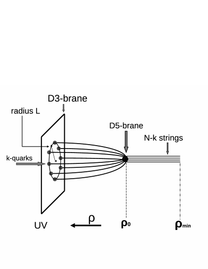
Figure 1: A baryon configuration with $k$-external quarks placed on a spherical shell of radius $L$ at the boundary of AdS space, each connected to the wrapped $Dp$-brane located at $\rho=\rho_{0}$ and $N-k$ straight strings ending at $\rho_{\rm min}$.

2 The holographic baryon vertex construction

In this section we review the holographic description of baryons in the general class of backgrounds presented in [8], as well as the study of their stability against small fluctuations. The first part generalizes the construction in [4, 5] to non-conformal cases like the Maldacena-Nuñez background that we will discuss in section 5.

We consider diagonal metrics of Lorentzian signature of the form

$$ds^{2}=G_{tt}dt^{2}+G_{xx}(dx^{2}+dy^{2}+dz^{2})+G_{\rho\rho}d\rho^{2}+R^{2}d\mathbb{M}_{p}^{2}\ ,$$ (2.1)

where $x,y$ and $z$ denote cyclic coordinates and $\rho$ denotes the radial direction playing the role of an energy scale in the dual gauge theory. It extends from the UV at $\rho\to\infty$ down to the IR at some minimum value $\rho_{\rm min}$ determined by the geometry.

It is convenient to introduce the functions

$$f(\rho)=-G_{tt}G_{xx}\ ,\qquad g(\rho)=-G_{tt}G_{\rho\rho}\ ,\qquad h(\rho)=G_{xx}G_{\rho\rho}\ ,$$ (2.2)

which for $AdS_{5}\times\mathbb{M}_{5}$ with radii $R$ read

$$f(\rho)=\rho^{4}\ ,\qquad g(\rho)=1\ ,\qquad h(\rho)=1\ .$$ (2.3)

As we have mentioned, a non-singlet baryon is described holographically in terms of a $Dp$-brane wrapping the internal manifold $\mathbb{M}_{p}$ with $k$ fundamental strings connecting it to the boundary at $\rho\rightarrow\infty$. The remaining $N-k$ straight strings go from the $Dp$-brane straight up at $\rho_{\rm min}$. The binding potential energy of the baryon is then given by $e^{-{\rm i}ET}=e^{{\rm i}S_{\rm cl}}$, where $S_{\rm cl}$ is the classical action of the holographic baryon. This action consists of three terms, the Nambu–Goto action for the strings stretching from the baryon vertex to the boundary at $\rho\rightarrow\infty$, the Nambu–Goto action for the straight strings stretching between the brane and $\rho_{\rm min}$ and the Dirac–Born–Infeld action for the $Dp$-brane

$$S_{F1}=-{1\over 2\pi}\int d\tau d\sigma\sqrt{-\det P(G_{\alpha\beta})}\ ,$$

$$S_{Dp}^{DBI}=-T_{p}\int_{\mathbb{R}\times\mathbb{M}_{p}}d^{p+1}\xi\,\sqrt{-\det P(G_{ab}+2\pi F_{ab}-B_{ab})}\ ,$$

where $F$ is the Born-Infeld field strength.

We first fix reparametrization invariance for each string by choosing

$$t=\tau\ ,\qquad\rho=\sigma\ .$$ (2.4)

For static solutions we consider the embedding of the $S^{2}$–sphere on the $D3$–brane in spherical coordinates $(r,\theta,\phi)$

$$r=r(\rho)\ ,\qquad(\theta,\phi)={\rm const.}\ ,$$ (2.5)

plus $\mathbb{M}_{p}\hbox{--angles}={\rm const.}$, supplemented by the boundary condition

$$\rho\left(L\right)=\infty\ .$$ (2.6)

Then, the Nambu–Goto action for the strings stretching from the baryon vertex to the boundary of AdS reads

$$S=-{T\over 2\pi}\int_{\rho_{0}}^{\infty}d\rho\,\sqrt{g(\rho)+f(\rho)r^{\prime 2}}\ ,$$ (2.7)

where $T$ denotes time and the prime denotes a derivative with respect to $\rho$. From the Euler–Lagrange equations of motion we obtain

$${fr_{\rm cl}^{\prime}\over\sqrt{g+fr_{\rm cl}^{\prime 2}}}=f_{1}^{1/2}\qquad\Longrightarrow\qquad r_{\rm cl}^{\prime}={\sqrt{f_{1}F}\over f}\ ,$$ (2.8)

where $\rho_{1}$ is the value of $\rho$ at the turning point of each string, $f_{1}\equiv f(\rho_{1}),\ f_{0}\equiv f(\rho_{0})$ and

$$F={gf\over f-f_{1}}\ .$$ (2.9)

The $N-k$ strings which extend from the baryon vertex to $\rho=\rho_{\rm min}$ are straight, since $r^{\prime}=0$ is a solution of the equations of motion (with $f_{1}=0$) and satisfies the boundary condition at the vertex. Integrating (2.8) we can express the radius of the spherical shell as

$$L=\sqrt{f_{1}}\int_{\rho_{0}}^{\infty}d\rho{\sqrt{F}\over f}\ .$$ (2.10)

Next we fix the reparametrization invariance for the wrapped $Dp$-brane by choosing

$$t=\tau\ ,\qquad\theta_{a}=\sigma_{\alpha}\ ,\quad\alpha=1,2,\dots,p\ .$$ (2.11)

Finally, inserting the solution for $r_{\rm cl}^{\prime}$ into (2.7) and subtracting the divergent energy of its constituents we can write the binding energy of the baryon as

$$E={k\over 2\pi}\left\{\int_{\rho_{0}}^{\infty}d\rho\sqrt{F}-\int_{\rho_{\rm min}}^{\infty}d\rho\sqrt{g}+{1-a\over a}\int_{\rho_{\rm min}}^{\rho_{0}}d\rho\sqrt{g}\ +\frac{2\pi}{aN}\,E_{Dp}\bigg{|}_{\rho=\rho_{0}}\right\}\ ,$$ (2.12)

where

$$a\equiv{k\over N}\ ,\qquad 0<a\leqslant 1\ .$$ (2.13)

The expressions for the length and the energy, (2.10) and (2.12), depend on the arbitrary parameter $\rho_{1}$ which should be expressed in terms of the baryon vertex position $\rho_{0}$. The most convenient way to find this is to impose that the net force at the baryon vertex is zero [29, 8]

$$\cos\Theta={1-a\over a}+\frac{2\pi}{aN}\frac{1}{\sqrt{g}}\,\partial_{\rho}E_{Dp}\bigg{|}_{\rho=\rho_{0}}\ ,$$ (2.14)

$$\cos\Theta=\sqrt{1-f_{1}/f_{0}}\ ,$$

where $\Theta$ is the angle between each of the $k$-strings and the $\rho$-axis at the baryon vertex, which determines $\rho_{1}$ in terms of $\rho_{0}$. An alternative derivation of this expression can be found by demanding that the physical length (2.10) does not depend on the arbitrary parameter $\rho_{1}$, in other words

$$\frac{\partial L}{\partial\rho_{1}}=0\Longrightarrow\frac{\partial\rho_{0}}{\partial\rho_{1}}=\frac{f_{1}^{\prime}}{2\tan\Theta}\sqrt{\frac{f_{0}}{g_{0}f_{1}}}\int_{\rho_{0}}^{\infty}d\rho\frac{\sqrt{gf}}{(f-f_{1})^{3/2}}\ .$$ (2.15)

Minimizing the energy (2.12) with respect to $\rho_{1}$ and using (2.15) we find the no-force condition (2.14). Using (2.10), (2.12) and (2.14) it is also possible to see that

$$\frac{dE}{d\rho_{0}}=\frac{k\sqrt{f_{1}}}{2\pi}\frac{dL}{d\rho_{0}}$$ (2.16)

which will be useful when we study the Maldacena-Nuñez background.

As we will see in the examples to follow, (2.14) has a solution for a parametric region of $(a,\rho_{0})$. However, in order to isolate parametric regions of physical interest a stability analysis of the classical solution should be performed, which further restricts the allowed region. We know from [8] that instabilities can only emerge from longitudinal fluctuations of the $k$ strings, since only these possess a non-divergent zero mode, which is a sign of instability. To study the fluctuations about the classical solution the embedding should be perturbed according to

$$r=r_{cl}+\delta r(\rho)\,,$$ (2.17)

and the Nambu-Goto action should be expanded to quadratic order in the fluctuations. $\delta r$ is then solved from the equation

$$\frac{d}{d\rho}\Bigl{(}\frac{gf}{F^{3/2}}\frac{d}{d\rho}\Bigr{)}\delta r=0$$ (2.18)

This has to be supplemented with the boundary condition for the $\delta r$ fluctuations, given by equation (3.12) in [8]

$$2(f-f_{1})\delta r^{\prime}+\delta r\,\Bigl{(}2f^{\prime}-\frac{f^{\prime}}{f}f_{1}-\frac{g^{\prime}}{g}(f-f_{1})\Bigr{)}=0\qquad{\rm at}\,\,\,\rho=\rho_{0}$$ (2.19)

As we will see in the examples to follow these conditions further restrict the parametric region $(a,\rho_{0})$ for which a classical non-singlet baryon solution exists.

3 The baryon vertex in $AdS_{5}\times Y_{5}$ manifolds

The holographic description of the baryon vertex in $AdS_{5}\times Y_{5}$ backgrounds with $Y_{5}$ an Einstein manifold bearing five-form flux is identical, in the probe brane approximation, to that in $AdS_{5}\times S^{5}$ [4, 5]. Therefore non-singlet states exist for the same number of fundamental strings $5N/8<k\leqslant N$. Spike solutions associated to the baryon vertices in the $AdS_{5}\times Y^{p,q}$ and $AdS_{5}\times T^{1,1}$ geometries have been discussed in [15] and [14], where it has been shown that they break all the supersymmetries. Therefore we are certain that the bound states found in the probe brane approximation will not become marginal due to supersymmetry once the backreaction is taken into account. In these two geometries we will switch on a magnetic flux that will dissolve D1 and D3-brane charges in the configuration. The vertex will then be described at finite ’t Hooft coupling in terms of D1-branes expanding into a fuzzy $S^{2}\times S^{2}$ submanifold of the $T^{1,1}$ for the Klebanov-Witten background and D3-branes expanding into a fuzzy $S^{2}$ submanifold of the $Y^{p,q}$ for the Sasaki-Einstein. The detailed microscopical analysis of these configurations will be performed in section 6 and the appendix respectively.

3.1 The D5-brane baryon vertex

In our conventions the $AdS_{5}\times Y_{5}$ metric reads

$$ds^{2}=\frac{\rho^{2}}{R^{2}}dx^{2}_{1,3}+\frac{R^{2}}{\rho^{2}}d\rho^{2}+R^{2}ds^{2}_{Y_{5}}~{},$$ (3.1)

with $R$ the radius of curvature in string units,

$$R^{4}=\frac{4\pi^{4}Ng_{s}}{{\rm Vol}(Y_{5})}~{}.$$ (3.2)

The $AdS_{5}\times Y_{5}$ flux is given by $F_{5}=(1+\star_{10}){\cal F}_{5}$, where

$${\cal F}_{5}=4\,R^{4}\,d{\rm Vol}(Y_{5})\ .$$ (3.3)

A D5-brane wrapping the whole $Y_{5}$ captures the $F_{5}$ flux, and it requires the addition of $N$ fundamental strings to cancel the tadpole

$$S^{CS}_{D5}=2\pi\,T_{5}\int_{\mathbb{R}\times Y_{5}}P[C_{4}]\wedge F=-2\pi\,T_{5}\int_{\mathbb{R}\times Y_{5}}P[F_{5}]\wedge A=-N\int dtA_{t}~{},$$ (3.4)

where $A$ is the Born-Infeld vector field. The DBI action is in turn given by

$$S^{DBI}_{D5}=-T_{5}\int_{\mathbb{R}\times Y_{5}}d^{6}\xi\,e^{-\phi}\sqrt{-{\rm det}P(G)}=-\frac{TN}{8\pi}\rho_{0}\ .$$ (3.5)

3.1.1 Classical solution

Given that the energy of the D5-brane is independent of the volume of the Einstein manifold the classical solution in the probe brane approximation is the one found in [4, 5] for $AdS_{5}\times S^{5}$. Making contact with the analysis in the previous section we now have

$$-G_{tt}=G_{xx}=G_{\rho\rho}^{-1}={\rho^{2}\over R^{2}}\ .$$ (3.6)

The radius and the energy are then given in terms of the position of the $D5$-brane $\rho_{0}$ and the turning point $\rho_{1}$ of each string, as

$$L={R^{2}\rho_{1}^{2}\over 3\rho_{0}^{3}}\ {\cal I}\ ,\qquad E={k\rho_{0}\over 2\pi}\left(-{\cal J}+{5-4a\over 4a}\right)\ ,$$ (3.7)

with ${\cal I}$, ${\cal J}$ the hypergeometric functions

$${\cal I}={{}_{2}F_{1}}\left({1\over 2},{3\over 4},{7\over 4};{r_{1}^{4}\over r_{0}^{4}}\right)\ ,\qquad{\cal J}={{}_{2}F_{1}}\left(-{1\over 4},{1\over 2},{3\over 4};{r_{1}^{4}\over r_{0}^{4}}\right)\,,$$ (3.8)

exactly as in $AdS_{5}\times S^{5}$. From (2.14) we find that the no-force condition on the $\rho$-axis yields

$$\rho_{1}=\rho_{0}(1-\lambda^{2})^{1/4}\ ,\qquad\lambda={5-4a\over 4a}\ ,\qquad a\equiv{k\over N}\ .$$ (3.9)

Given that $\lambda<1$ a baryon configuration exists for $a>a_{<}$ with $a_{<}={5\over 8}$ Finally, the binding energy in terms of the physical length of the baryon reads

$$E=-{R^{2}\over 2\pi L}{k\sqrt{1-\lambda^{2}}\over 3}\left({\cal J}-{5-4a\over 4a}\right){\cal I}\ .$$ (3.10)

Thus it has both the expected behavior with $1/L$ dictated by conformal invariance and the non-analyticity of square-root branch cut type in the ’t Hooft parameter [6, 4, 27]. We would also like to point out that our string and brane configurations satisfy the Sasaki-Einstein constrains in the way studied in [30] and therefore our solutions are in this sense valid.

3.1.2 Stability analysis

Again as in $AdS_{5}\times S^{5}$ [8] the study of the stability against longitudinal fluctuations gives

$$\delta r(\rho)=A\int_{\rho}^{\infty}d\rho{\rho^{2}\over(\rho^{4}-\rho_{1}^{4})^{3/2}}={A\over 3\rho^{3}}\ {{}_{2}F_{1}}\left({3\over 4},{3\over 2},{7\over 4};{\rho_{1}^{4}\over\rho^{4}}\right)$$ (3.11)

as the solution of equation (2.18). Substituting (3.9) and (3.11) in the boundary equation (2.19) the following transcendental equation must be satisfied

$${{}_{2}F_{1}}\left({3\over 4},{3\over 2},{7\over 4};1-\lambda^{2}\right)={3\over 2\lambda(1+\lambda^{2})}\ .$$ (3.12)

Using (3.9) and (3.12) a critical value for $a$ is found numerically, $a\simeq 0.813$ , below which the system becomes unstable.

The conclusion of this analysis is that in the probe brane approximation non-singlet baryons with $0.813<k\leqslant N$ may exist for all Einstein internal manifolds bearing five-form flux. In the next subsection we take the internal manifold to be Sasaki-Einstein and we switch on an instantonic magnetic flux proportional to the Kähler form. The $T^{1,1}$ and $S^{5}$ cases will be treated as particular examples, taking due care of the different periodicities. The energy of the D5-brane will depend then on both the magnetic flux and the radius of $AdS$, and the same calculation above shows that non-singlet states exist as long as the number of quarks is larger than a minimum value that depends now on the volume of the $Y^{p,q}$. In fact the largest minimum value is reached for the $S^{5}$, contrary to our expectations that non-singlet baryons would be more restricted in less supersymmetric backgrounds. We review some basic facts about the geometry of $Y^{p,q}$ manifolds suitable for this study in the Appendix.

3.2 The baryon vertex in $AdS_{5}\times Y^{p,q}$ with magnetic flux

Let us take the $AdS_{5}\times Y^{p,q}$ geometry and add a magnetic flux

$$F={\cal N}J\,,$$ (3.13)

with $J$ the Kähler form of the 4 dimensional Kähler-Einstein submanifold of the $Y^{p,q}$, which solves the equations of motion. As compared to the analysis in the previous subsection the presence of the magnetic flux will turn the parametric region for which a classical solution exists to depend on $(a,\rho_{0},{\cal N})$.

For a non-vanishing ${\cal F}$ as above the energy of the D5-brane wrapped on the $Y^{p,q}$ is modified according to

$$E_{D5}={N\over 8\pi}\rho_{0}\left(1+\frac{4\pi^{2}{\cal N}^{2}}{R^{4}}\right)$$ (3.14)

where we have used (A.11), and the fact that $J$ is self-dual and the determinant inside the square root is a perfect square.

This magnetic flux dissolves irrational D1-brane charge in the $Y^{p,q}$, as inferred from the coupling

$$S_{D5}^{CS}=\frac{1}{2}(2\pi)^{2}T_{5}\int_{\mathbb{R}\times Y^{p,q}}C_{2}\wedge F\wedge F=\frac{{\cal N}^{2}}{8}\frac{q^{2}[2p+(4p^{2}-3q^{2})^{1/2}]}{p^{2}[3q^{2}-2p^{2}+p(4p^{2}-3q^{2})^{1/2}]}\,T_{1}\int_{\mathbb{R}\times S^{1}_{\psi}}C_{2}$$ (3.15)

This implies that the configuration will not allow a complementary description in terms of D1-branes expanding into a fuzzy 4 dimensional submanifold of the $Y^{p,q}$. We will see however that it will be possible to provide such a description in terms of D3-branes expanding into a fuzzy 2-sphere submanifold of the $Y^{p,q}$. In this case the magnetic flux that needs to be switched on will be proportional to the Kähler form on the $S^{2}$. We postpone this discussion to the Appendix.

In the $T^{1,1}$ case (see Appendix A.2 for a brief discussion of the $T^{1,1}$ geometry) our ansatz (3.13) dissolves ${\cal N}^{2}/9$ D1-brane charge in the $T^{1,1}$, as implied by

$$S_{D5}^{CS}=\frac{1}{2}(2\pi)^{2}T_{5}\int_{\mathbb{R}\times T^{1,1}}C_{2}\wedge F\wedge F=\frac{{\cal N}^{2}}{9}T_{1}\int_{\mathbb{R}\times S^{1}_{\psi}}C_{2}$$ (3.16)

where we have used the second condition in (A.18). But in this case ${\cal N}^{2}/9$ is an integer due to Dirac quantization condition plus the first equation in (A.18). In this case a microscopical description in terms of expanding D1-branes will make sense, as we will show explicitly in section 6.

Note that in fact for the $T^{1,1}$ we can take a more general ansatz for the magnetic flux, namely $F={\cal N}_{1}\,J_{1}\,+\,{\cal N}_{2}\,J_{2}$, with $J_{1}$, $J_{2}$ the Kähler forms on each of the $S^{2}$’s contained in the $T^{1,1}$. In this case the magnetic flux is dissolving ${\cal N}_{1}/3$ and ${\cal N}_{2}/3$ D3-brane charge in each $S^{2}$, and ${\cal N}_{1}{\cal N}_{2}/9$ D1-brane charge in $S^{2}\times S^{2}$, as inferred from the couplings

$$S_{D5}^{CS}=2\pi\,T_{5}\int_{\mathbb{R}\times T^{1,1}}C_{4}\wedge F=\frac{{\cal N}_{1}}{3}\,T_{2}\int_{{\mathbb{R}\times S^{1}_{\psi}\times S_{2}^{2}}}C_{4}+\frac{{\cal N}_{2}}{3}\,T_{2}\int_{{\mathbb{R}\times S^{1}_{\psi}\times S_{2}^{1}}}C_{4}$$ (3.17)

and

$$S_{D5}^{CS}=\frac{1}{2}(2\pi)^{2}T_{5}\int_{\mathbb{R}\times T^{1,1}}C_{2}\wedge F\wedge F=\frac{{\cal N}_{1}{\cal N}_{2}}{9}\,T_{1}\int_{\mathbb{R}\times S^{1}_{\psi}}C_{2}\ .$$ (3.18)

Therefore ${\cal N}_{1},{\cal N}_{2}\in 3\mathbb{Z}$, in agreement with Dirac quantization condition, as implied from (A.18). In this case the energy of the D5 is modified according to

$$E_{D5}={N\over 8\pi}\rho_{0}\sqrt{1+\frac{4\pi^{2}{\cal N}_{1}^{2}}{R^{4}}}\sqrt{1+\frac{4\pi^{2}{\cal N}_{2}^{2}}{R^{4}}}\ .$$ (3.19)

Coming back to the general case for $Y^{p,q}$ manifolds, $F={\cal N}J$, with $J$ the Kähler form of the 4 dimensional Kähler-Einstein submanifold of the $Y^{p,q}$, from (2.14) we find that the no-force condition on the $\rho$-axis yields

$$\rho_{1}=\rho_{0}(1-\lambda_{\rm eff}^{2})^{1/4}\ ,\qquad\lambda_{\rm eff}={5-4a_{\rm eff}\over 4a_{\rm eff}}\ ,$$ (3.20)

where $a_{\rm eff}$ includes now the magnetic flux

$$a_{\rm eff}\equiv{a\over 1+{4\pi^{2}{{\cal N}^{2}}\over 5R^{4}}}\ .$$ (3.21)

Given that $\lambda_{\rm eff}<1$ a baryon configuration exists for

$$a_{\rm eff}>a_{<}\qquad{\rm with}\qquad a_{<}={5\over 8}+\frac{\pi^{2}{\cal N}^{2}}{2R^{4}}\,.$$ (3.22)

In terms of the volume of the $Y^{p,q}$ this reads

$$a_{<}=\frac{5}{8}+\frac{{\cal N}^{2}}{8\pi^{2}\,N}{\rm Vol}(Y^{p,q})\ ,$$ (3.23)

so the bound depends now on the volume of the internal manifold. The largest volume given by the $Y^{p,q}$ metrics occurs for the $Y^{2,1}$, for which ${\rm Vol}(Y^{2,1})\approx 0.29\pi^{3}$. Therefore we have that $\pi^{3}={\rm Vol}(S^{5})>16/27\,\pi^{3}={\rm Vol}(T^{1,1})>{\rm Vol}(Y^{2,1})$ and $a_{<}$ is maximum for the $S^{5}$, the maximally supersymmetric case. Note that since $a_{\rm eff}\leqslant 1$ there is also a bound on the instanton number, namely

$$a_{<}\leqslant 1\quad\Rightarrow\quad\frac{{\cal N}^{2}}{R^{4}}\leqslant{3\over 4\pi^{2}}\simeq 0.0761\ .$$ (3.24)

Finally, the binding energy in terms of the physical length of the baryon reads

$$E=-{R^{2}\over 2\pi L}{k\sqrt{1-\lambda_{\rm eff}^{2}}\over 3}\left({\cal J}-{5-4a_{\rm eff}\over 4a_{\rm eff}}\right){\cal I}\ .$$ (3.25)

3.2.1 Stability analysis

The study of the stability against longitudinal fluctuations gives again $\delta r(\rho)$ as in (3.11) where now ${{}_{2}F_{1}}(a,b,c;x)$ must satisfy [8]

$${{}_{2}F_{1}}\left({3\over 4},{3\over 2},{7\over 4};1-\lambda_{\rm eff}^{2}\right)={3\over 2\lambda_{\rm eff}(1+\lambda_{\rm eff}^{2})}\ .$$ (3.26)

The critical value for $a_{\rm eff}$ that is found numerically is again $a_{\rm eff}\simeq 0.813$ , below which the system becomes unstable. This improves the above bound for the instanton number, in comparison to the ’t Hooft coupling, to

$${{\cal N}^{2}\over R^{4}}\lesssim 0.00291\ ,$$ (3.27)

that should be respected for the classical configuration not only to exist, but also to be perturbatively stable. Thus, the stability analysis sets a low bound for $a$ which is still less than unity.

4 The baryon vertex in $\beta$-deformed backgrounds

The description of the baryon vertex in these backgrounds is essentially identical to the one performed in the previous section. Even though the $C_{2}$ and $B_{2}$ potentials are non-vanishing the tadpole introduced with the brane has still charge $N$, so it has to be compensated with the same number of fundamental strings attached. Moreover, the energy of the D5-brane wrapped on the deformed $S^{5}$ is the same as the one wrapped on the $S^{5}$. Therefore we find the same bound for the number of quarks that can form non-singlet baryons.

We discuss the general case of multi ${\hat{\gamma}}_{i}$-deformations [22], from which the one- parameter Lunin-Maldacena background [21] is obtained for all ${\hat{\gamma}}_{i}$ equal. As we have mentioned, in this background the baryon vertex is described in terms of a D5-brane wrapped on the deformed $S^{5}$, with $N$ fundamental strings attached. In the last subsection we will switch on a magnetic flux that on the one hand will increase the parametric space on which classical solutions exist and on the other hand will allow a complementary description in terms of expanding D3-branes suitable for the discussion of the finite ’t Hooft coupling regime of the dual gauge theory.

The multi-${\hat{\gamma}}_{i}$ deformed background reads in string frame [22]

$$ds^{2} = R^{2}\left[ds^{2}_{AdS_{5}}+\sum_{i}\left(d\mu_{i}^{2}+{\cal G}\mu_{i}^{2}d\phi_{i}^{2}\right)+{\cal G}\mu_{1}^{2}\mu_{2}^{2}\mu_{3}^{2}\big{(}\sum_{i}{\hat{\gamma}}_{i}d\phi_{i}\big{)}^{2}\right]\,,$$ (4.1)

$$e^{2\phi} = {\cal G}\ ,\qquad{\cal G}^{-1}=1+{\hat{\gamma}}_{3}^{2}\,\mu_{1}^{2}\mu_{2}^{2}+{\hat{\gamma}}_{1}^{2}\,\mu_{2}^{2}\mu_{3}^{2}+{\hat{\gamma}}_{2}^{2}\,\mu_{3}^{2}\mu_{1}^{2}\,.$$

$$B_{2} = R^{2}{\cal G}\,({\hat{\gamma}}_{3}\,\mu_{1}^{2}\mu_{2}^{2}\,d\phi_{1}\wedge d\phi_{2}+{\hat{\gamma}}_{1}\,\mu_{2}^{2}\mu_{3}^{2}\,d\phi_{2}\wedge d\phi_{3}+{\hat{\gamma}}_{2}\,\mu_{3}^{2}\mu_{1}^{2}\,d\phi_{3}\wedge d\phi_{1})\,,$$

$$C_{2} = -4R^{2}\omega_{1}\wedge({\hat{\gamma}}_{1}d\phi_{1}+{\hat{\gamma}}_{2}d\phi_{2}+{\hat{\gamma}}_{3}d\phi_{3})\,,$$

$$C_{4} = \omega_{4}+4R^{4}{\cal G}\,\omega_{1}\,\wedge d\phi_{1}\wedge d\phi_{2}\wedge d\phi_{3}\,,$$

where $\mu_{i}$ and $\phi_{i}$ parameterize a deformed five-sphere, so that we can write:

$$\begin{gathered}\mu_{1}=\cos\alpha\,,\qquad\mu_{2}=\sin\alpha\cos\theta\,,\qquad\mu_{3}=\sin\alpha\sin\theta\,,\qquad\sum_{i=1}^{3}\mu_{i}^{2}=1\,,\\ (\alpha,\theta)\in[0,\pi/2]\ ,\qquad d\omega_{1}=\cos\alpha\sin^{3}\alpha\sin\theta\cos\theta d\alpha\wedge d\theta\,,\qquad d\omega_{4}=\omega_{AdS_{5}}\,.\end{gathered}$$ (4.2)

For equal ${\hat{\gamma}}_{i}$ parameters ${\hat{\gamma}}_{1}={\hat{\gamma}}_{2}={\hat{\gamma}}_{3}={\hat{\gamma}}$, ${\hat{\gamma}}$ is related to the deformation parameter $\beta$ of the gauge theory through [31]:

$${\hat{\gamma}}=R^{2}\ \beta\,.$$ (4.3)

4.1 The D5-brane baryon vertex

Let us now consider a D5-brane wrapping the deformed $S^{5}$ in (4.1). This brane captures the $F_{5}-F_{3}\wedge B_{2}$ flux of the background but still requires $N$ fundamental strings to cancel the tadpole

$$S_{D5}^{CS} = 2\pi\,T_{5}\int_{\mathbb{R}\times{\tilde{S}}^{5}}P\left[C_{4}-C_{2}\wedge B_{2}\right]\wedge F=-2\pi\,T_{5}\int_{\mathbb{R}\times{\tilde{S}}^{5}}P\left[F_{5}-F_{3}\wedge B_{2}\right]\wedge A=$$ (4.4)

$$= -N\int dtA_{t}$$

since

$$F_{5}-F_{3}\wedge B_{2}=\omega_{AdS_{5}}+4R^{4}\,d\omega_{1}\wedge d\phi_{1}\wedge d\phi_{2}\wedge d\phi_{3}~{},$$ (4.5)

as in the $AdS_{5}\times S^{5}$ case. Therefore the CS part of the action is undeformed. The DBI action is in turn given by

$$S_{D5}^{DBI}=-T_{5}\int_{\mathbb{R}\times\tilde{S}^{5}}d^{6}\xi\ e^{-\phi}\sqrt{-\det P\left(G+2\pi F-B_{2}\right)}\,.$$ (4.6)

For $F=0$ the determinant of the pull-back of $G-B_{2}$ can be written as

$$\Delta_{1}=G_{tt}G_{\alpha\alpha}G_{\theta\theta}\det{\Gamma}~{},$$ (4.7)

where $\Gamma$ is a $3\times 3$ matrix of the form $G_{ab}-B_{ab}$ for the three $U(1)$ directions. We then get

$$\Delta_{1}=G_{tt}\,R^{10}\sin^{6}{\alpha}\cos^{2}{\alpha}\sin^{2}{\theta}\cos^{2}{\theta}\,{\cal G}\ ,$$ (4.8)

such that the DBI action remains also undeformed.

Given that the $AdS$ part of the background remains untouched by the deformation the contribution of the fundamental strings stretching from the D5 to the boundary of $AdS$ is the same as in the undeformed case. The only issue here would be that the binding energy was modified due to the dependence of the D5-brane on the deformation parameter. We have shown however that this dependence drops out both in the CS and DBI actions. Therefore the size and binding energy of the baryon remain undeformed, and coincide with those in ${\cal N}=4$. The classical solution and its stability analysis are therefore identical to those performed in section 3. Last but not least, we should mention that for marginally-deformed backgrounds there are cases on which the classical solution coincides with ${\cal N}=4$, does not depend on the deformation parameter, but the stability analysis even for the conformal case requires an upper value on the imaginary part of the deformation parameter $\sigma$ as in the case of mesons [32].

4.1.1 Adding a magnetic flux

Finally we can switch on a magnetic flux $F={\cal N}J$, with ${\cal N}\in{\mathbb{Z}}/2$ and $J$ the Kähler form of the $S^{2}$ parameterized by $(\alpha,\theta)$, dissolving $2{\cal N}$ units of D3-brane charge in the baryon. This will allow a microscopical description in terms of expanding D3-branes from which the finite ’t Hooft coupling region can be studied. The DBI action changes as

$$S^{DBI}_{D5}=-\frac{TN}{8\pi}\rho_{0}\sqrt{1+\frac{4\pi^{2}{\cal N}^{2}}{R^{4}}}\ .$$ (4.9)

In the presence of a magnetic flux the minimum number of quarks forming a non-singlet baryon is modified and there is a maximum on the magnetic flux that can be dissolved in the baryon, in parallel with what we have found in the previous section.

5 The baryon vertex in the Maldacena–Nuñez background

The Maldacena-Nuñez background [17] is a solution to Type IIB supergravity dual to a ${\cal N}=1$ supersymmetric confining gauge theory. It can be obtained as a solution of seven dimensional gauged supergravity [33], uplifted to ten dimensions. Given that this background is confining we expect that the universality of the baryon vertex configurations found in the previous conformal examples (in the absence of a magnetic flux) is lost. This is indeed confirmed by the analysis in this section.

5.1 The Maldacena–Nuñez background

The ten-dimensional metric reads in the string frame

$$ds^{2}_{10}\,=\,e^{\phi}\,\,\Big{[}\,dx^{2}_{1,3}\,+g_{s}N\Bigl{(}\,e^{2h}\,\big{(}\,d\theta_{1}^{2}+\sin^{2}\theta_{1}d\phi_{1}^{2}\,\big{)}\,+\,d\rho^{2}\,+\,{1\over 4}\,(w^{i}-A^{i})^{2}\Bigr{)}\,\Big{]}\,\,,$$ (5.1)

where $\phi$ is the dilaton, $h$ is a function of the radial coordinate $\rho$, the one-forms $A^{i}$ $(i=1,2,3)$ are the components of the non-abelian gauge vector field of the seven-dimensional gauged supergravity,

$$A^{1}\,=\,-a(\rho)d\theta_{1}\,,\,\,\,\,\,\,\,\,\,A^{2}\,=\,a(\rho)\sin\theta_{1}d\phi_{1}\,,\,\,\,\,\,\,\,\,\,A^{3}\,=\,-\cos\theta_{1}d\phi_{1}\,,$$ (5.2)

and the $w^{i}$’s are the right-invariant Maurer-Cartan dreibeins of $SU(2)$, satisfying $dw^{i}=-{1\over 2}\,\varepsilon_{ijk}\,w^{j}\wedge w^{k}$. They define a three-sphere that can be parameterized as

$$w^{1} = \cos\psi\,d\theta_{2}\,+\,\sin\psi\sin\theta_{2}\,d\phi_{2}\,\,,$$ (5.3)

$$w^{2} = -\sin\psi\,d\theta_{2}\,+\,\cos\psi\sin\theta_{2}\,d\phi_{2}\,\,,$$

$$w^{3} = d\psi\,+\,\cos\theta_{2}\,d\phi_{2}\,\,.$$

The angles $\theta_{\alpha},\phi_{\alpha}\ ,\alpha=1,2$ and $\psi$ take values in the intervals $\theta_{i}\in[0,\pi]$, $\phi_{i}\in[0,2\pi]$ and $\psi\in[0,4\pi]$. The functions $a(\rho)$, $h(\rho)$ and the dilaton $\phi(\rho)$ are given by

$$a(\rho)={2\rho\over\sinh 2\rho}\ ,\qquad e^{2h}=\rho\coth 2\rho\,-\,{\rho^{2}\over\sinh^{2}2\rho}\,-\,{1\over 4}\ ,\quad$$ (5.4)

$$e^{2\phi}=e^{-2\phi_{0}}\,{\sinh 2\rho\over 2e^{h}}\equiv e^{-2\phi_{0}}\Lambda(\rho)\ ,\qquad e^{2\phi_{0}}=g_{s}N\ .$$ (5.5)

In particular, $\Lambda(\rho)$ satisfies

$$\Lambda(\rho)\simeq\frac{e^{2\rho}}{4\sqrt{\rho}}\ ,\quad{\rm when}\quad\rho\gg 1$$ (5.6)

and

$$\Lambda(\rho)\simeq 1+\frac{8\rho^{2}}{9}+{\cal O}(\rho^{4})\ ,\quad{\rm when}\quad\rho\ll 1\ .$$ (5.7)

The solution also includes a Ramond-Ramond three-form given by

$$F_{3}\,=\,{g_{s}N\over 4}\left\{-\,\big{(}\,w^{1}-A^{1}\,\big{)}\wedge\big{(}\,w^{2}-A^{2}\,\big{)}\wedge\big{(}\,w^{3}-A^{3}\,\big{)}\,+\,\,\,\sum_{i}\,F^{i}\wedge\big{(}\,w^{i}-A^{i}\,\big{)}\right\}\,\,,$$ (5.8)

where $F^{i}$ is the field strength of the $SU(2)$ gauge field $A^{i}$, defined as $F^{i}\,\equiv\,dA^{i}\,+\,{1\over 2}\varepsilon_{ijk}\,A^{j}\wedge A^{k}$.

5.2 The D3-brane baryon vertex

A D3-brane wrapping the 3-sphere parameterized by $(\theta_{2},\phi_{2},\psi)$ introduces a tadpole that needs to be canceled through the addition of $N$ fundamental strings

$$S_{D3}^{CS}=2\pi\,T_{3}\int_{\mathbb{R}\times S^{3}}C_{2}\wedge F=-2\pi\,T_{3}\int_{\mathbb{R}\times S^{3}}F_{3}\wedge A=-N\int dt\,A_{t}\ .$$ (5.9)

The DBI action of this D3-brane is given by:

$$S_{D3}^{DBI} = -T_{3}\int_{\mathbb{R}\times S^{3}}d^{4}\xi\,e^{-\phi}\sqrt{-\det P(G)}=-\frac{TN}{4\pi}\sqrt{\Lambda(\rho_{0})}\ .$$ (5.10)

Particularizing to this background the size of the vertex given by (2.10) we find

$$L=\sqrt{g_{s}N}\int_{\rho_{0}}^{\infty}\frac{d\rho}{\sqrt{\Lambda(\rho)/\Lambda(\rho_{1})-1}}\ ,$$ (5.11)

which is a decreasing function of $\rho_{0}$. The binding energy of the baryon is in turn given by

$$E=\frac{k}{2\pi}\Bigl{\{}\int_{\rho_{0}}^{\infty}d\rho\frac{\Lambda(\rho)}{\sqrt{\Lambda(\rho)-\Lambda(\rho_{1})}}-\int_{\rho_{\rm min}}^{\infty}d\rho\,\sqrt{\Lambda(\rho)}+\frac{1-a}{a}\int_{\rho_{\rm min}}^{\rho_{0}}d\rho\,\sqrt{\Lambda(\rho)}+\frac{1}{2a}\sqrt{\Lambda(\rho_{0})}\Bigr{\}}\ .$$ (5.12)

Both integrals receive most of their contributions from the region $\rho\approx\rho_{1}$ so it can be seen that $E$ is linearly proportional to $L$ [18]. Also, from (2.16) we see that $E$ and $L$ share the same dependence on the position of the vertex:

$$\frac{dE}{d\rho_{0}}=\frac{k\sqrt{\Lambda_{1}}}{2\pi\sqrt{g_{s}N}}\frac{dL}{d\rho_{0}}\,.$$ (5.13)

The net-force condition is now

$$\cos\Theta=\frac{1-a}{a}+\frac{1}{4a}\partial_{\rho}\ln\Lambda(\rho)\bigg{|}_{\rho=\rho_{0}}\ ,\qquad\cos\Theta=\sqrt{1-\frac{\Lambda_{1}}{\Lambda_{0}}}\ .$$ (5.14)

Taking into account that $\partial_{\rho}\ln\Lambda(\rho)$ satisfies $\partial_{\rho}\ln\Lambda(\rho)\lesssim 2-1/(2\rho)+{\cal O}(1/\rho^{2})$ in the UV we find that $a>a_{<}$ with $a_{<}=3/4$. Therefore the minimum value of the number of quarks is restricted with respect to the one found in the previous conformal examples, in agreement with our expectations.

5.2.1 Stability analysis

The study of the stability against longitudinal fluctuations gives

$$\delta r(\rho)=A\,g_{s}N\int_{\rho}^{\infty}d\rho\,\frac{\Lambda}{(\Lambda-\Lambda_{1})^{3/2}}\ ,$$ (5.15)

as the solution to equation (2.18). Substituting in the boundary equation (2.19) we find

$$2(\Lambda-\Lambda_{1})\delta r^{\prime}+\Lambda^{\prime}(\rho)\,\delta r=0\quad{\rm at}\quad\rho=\rho_{0}\,,$$ (5.16)

and using (5.14) we can write

$$a\,(\cos\Theta+\frac{a-1}{a})\cos\Theta\ {\cal Z}=\frac{1}{2}$$ (5.17)

where

$${\cal Z}\equiv\sqrt{\Lambda_{0}}\int_{\rho_{0}}^{\infty}d\rho\,\frac{\Lambda}{(\Lambda-\Lambda_{1})^{3/2}}\ ,\quad{\rm and}\quad\Lambda_{1}=\Lambda_{0}\sin^{2}\Theta\ .$$ (5.18)

From (5.17) we can now solve for $a$. Note that using (2.15) we find that

$$\frac{\partial\rho_{0}}{\partial\rho_{1}}={\frac{1}{2}}{\cal Z}\cos\Theta\ \partial_{\rho}\ln\Lambda(\rho)|_{\rho=\rho_{1}}$$ (5.19)

from where

$${\cal Z}\cos\Theta=\frac{2}{\partial_{\rho_{0}}\ln\Lambda(\rho_{0})}\in[1,\infty)\ .$$ (5.20)

From (5.17) and (5.19) we then find $\displaystyle a\geqslant{\frac{1}{2}}+\frac{1}{4{\cal Z}\cos\theta}\Longrightarrow a\geqslant{\frac{1}{2}}+\frac{\partial_{\rho_{0}}\ln\Lambda(\rho_{0})}{8}$. Thus, the stability analysis does not improve the bound imposed by the existence of a classical solution, in contrast to what happened in the conformal examples previously discussed.

5.2.2 Adding a magnetic flux

Finally, in order to compare with the microscopical analysis in section 6.3 we add a magnetic flux to the baryon proportional to the Kähler form on the 2-sphere parameterized by $(\theta_{2},\phi_{2})$, $F={\cal N}J$, with ${\cal N}\in 2\mathbb{Z}$. This flux dissolves ${\cal N}/2$ units of D1-brane charge in the $S^{3}$. The energy of the baryon is modified according to

$$E_{D3}=\frac{N}{4\pi}\sqrt{\Lambda(\rho_{0})+\frac{4\pi^{2}{\cal N}^{2}}{g_{s}N}}\ .$$ (5.21)

As in the previous cases the magnetic flux changes the minimum bound for the number of quarks in the baryon. Moreover the flux has an upper bound.

6 The microscopical description

In the previous sections we have discussed generalizations of the baryon vertex constructions to allow a magnetic flux dissolving lower dimensional brane charge in the configuration. By analogy with Myers dielectric effect [34, 28] we expect that a complementary description in terms of lower dimensional branes expanding into fuzzy baryons should then be possible. This would be the “microscopical” realization of the “macroscopical” baryons with magnetic flux that we have just described. The interesting thing about the microscopical description is that it allows to explore the finite ’t Hooft coupling region, and this is especially relevant in those cases in which the baryons are non-supersymmetric, like those considered in this paper, and are therefore not preserved by a BPS condition.

It is well known that the macroscopical and microscopical descriptions have complementary ranges of validity [28]. While the first is valid in the supergravity limit the second is a good description when the mutual separation of the expanding branes is much smaller than the string length, such that they can be taken to be coincident and therefore described by the $U(n)$ effective action constructed by Myers [28]. For $n$ D$q$-branes expanded into an $r$-dimensional manifold of radius $R$, the volume per brane can be estimated as $R^{r-q}/n$, which must then be much smaller than $l_{s}^{r-q}$. Thus the condition

$$R<<n^{\frac{1}{r-q}}\,l_{s}\,,$$ (6.1)

sets the regime of validity of the microscopical description. The macroscopical description is in turn valid when $R>>1$. Therefore both descriptions are complementary for finite $n$, but should agree in the large $n$ limit, where they have a common range of validity. The limit (6.1) is especially appealing in backgrounds with a CFT dual, like the AdS spacetimes that we have considered in this paper. Indeed, in terms of the ’t Hooft parameter of the dual CFT the condition (6.1) reads

$$\lambda<<n^{\frac{4}{r-q}}\,.$$ (6.2)

The fact that $\lambda$ can be finite opens up the possibility of accessing the finite ’t Hooft coupling region of the dual CFT through the microscopical study of the corresponding dual brane system.

Dielectric branes expanding into fuzzy manifolds have been extensively studied in the literature. From (6.2) the lower the dimensionality of the expanding branes the smaller the ’t Hooft parameter can get. However for the manifolds that we have discussed in this paper it will not always be possible to provide a description in terms of expanding D1-branes. This is the case for the $Y^{p,q}$ Sasaki-Einstein geometries, in which the natural microscopical description would be in terms of D1-branes wrapped on the Reeb vector direction and expanding into the remaining four dimensional Kähler-Einstein manifold. We are however not aware of a fuzzy realization of these manifolds besides the $CP^{2}$ case. Moreover, as we have seen, the number of D1-branes in the macroscopical description is irrational, while this should be an integer in the microscopical description. Still, we will be able to provide a (less) microscopical description in terms of D3-branes expanding into a fuzzy 2-sphere. For the ${\hat{\gamma}}_{i}$ deformed backgrounds the natural thing is to dissolve D3-branes wrapped on the $(T^{1})^{3}$ through the addition of a magnetic flux proportional to the Kähler form on the $S^{2}$, as we did in section 4.1. The microscopical description will then be in terms of D3-branes expanding into a fuzzy $S^{2}$.

We start in section 6.1 with the analysis of the $AdS_{5}\times T^{1,1}$ background, for which a description in terms of D1-branes expanding into a fuzzy $S^{2}\times S^{2}$ manifold can be done. As we will see this description exactly matches the macroscopical description in section 3.2. The extension to arbitrary $Y^{p,q}$ manifolds is more technical and it is postponed to the Appendix. In section 6.2 we discuss the ${\hat{\gamma}}_{i}$ deformed backgrounds. We end with the Maldacena-Nuñez analysis in section 6.3, in terms of D1-branes expanding into a fuzzy $S^{2}$ baryon.

6.1 The $AdS_{5}\times T^{1,1}$ background: D1-branes into fuzzy $S^{2}\times S^{2}$

The DBI action describing the dynamics of $n$ coincident D1-branes is given by [28]

$$S^{DBI}_{nD1}=-T_{1}\int d^{2}\xi\,{\rm STr}\Bigl{\{}e^{-\phi}\sqrt{|{\rm det}\Bigl{(}P[E_{\mu\nu}+E_{\mu i}(Q^{-1}-\delta)^{i}{}_{j}E^{jk}E_{k\nu}]\Bigr{)}{\rm det}Q|}\Bigr{\}}$$ (6.3)

where $E=G-B_{2}$ and

$$Q^{i}{}_{j}=\delta^{i}{}_{j}+\frac{i}{2\pi}[X^{i},X^{k}]E_{kj}\,.$$ (6.4)

Let us take the D1-branes wrapped on the $U(1)$ fibre direction $\psi$ in (A.16) and expanding into the fuzzy $S^{2}\times S^{2}$ submanifold parameterized by $(\theta,\phi)$ and $(\omega,\nu)$.

Using Cartesian coordinates for each $S^{2}$ we can impose the condition

$$\sum_{i=1}^{3}(x^{i})^{2}=1$$ (6.5)

at the level of matrices if the $X^{i}$ are taken in the irreducible totally symmetric representation of order $m$, with dimension $n=m+1$,

$$X^{i}=\frac{1}{\sqrt{m(m+2)}}\,J^{i}$$ (6.6)

with $J^{i}$ the generators of $SU(2)$, satisfying $[J^{i},J^{j}]=2i\varepsilon_{ijk}J^{k}$. Labeling with $m_{1}$, $m_{2}$ the irreps for each $S^{2}$ we have that the total number of expanding branes $n=(m_{1}+1)(m_{2}+1)$, and substituting in the DBI action

$$S_{nD1}^{DBI}=-T_{1}\int d^{2}\xi\sqrt{-G_{tt}G_{\psi\psi}}\ \rm{Str}\sqrt{\det Q}$$ (6.7)

we find

$$E_{nD1}=\frac{N\rho_{0}}{8\pi}\frac{(m_{1}+1)(m_{2}+1)}{\sqrt{m_{1}(m_{1}+2)m_{2}(m_{2}+2)}}\sqrt{1+\frac{36\pi^{2}m_{1}(m_{1}+2)}{R^{4}}}\sqrt{1+\frac{36\pi^{2}m_{2}(m_{2}+2)}{R^{4}}}$$ (6.8)

where

$${\rm det}\,Q=\Bigl{(}1+\frac{R^{4}}{36\pi^{2}m_{1}(m_{1}+2)}\Bigr{)}\Bigl{(}1+\frac{R^{4}}{36\pi^{2}m_{2}(m_{2}+2)}\Bigr{)}\mathbb{I}$$ (6.9)

and the $(m_{1}+1)(m_{2}+1)$ factor comes from computing the symmetrized trace. This expression is exact in the limit

$$R>>1\,,\qquad m>>1\,,\qquad{\rm with}\qquad\frac{R^{2}}{m}={\rm finite}$$ (6.10)

(see section 5.1 of [35] for the detailed discussion). Taking the large $m_{1}$, $m_{2}$ limit we find perfect match with the macroscopical result given by (3.19) if $m_{1}\sim{\cal N}_{1}/3$, $m_{2}\sim{\cal N}_{2}/3$, in agreement with (A.18).

6.1.1 The F-strings in the microscopical description

An essential part of the baryon vertex are the fundamental strings that stretch from the D$p$-brane to the boundary of $AdS_{5}$. As we show in this section they arise from the non-Abelian CS action.

The CS action for $n$ coincident D1-branes is given by

$$S_{CS}=\int d^{2}\xi\,{\rm STr}\Bigl{\{}P\Bigl{(}e^{\frac{i}{2\pi}(i_{X}i_{X})}\,\sum_{q}C_{q}\,\,e^{-B_{2}}\Bigr{)}e^{2\pi F}\Bigr{\}}\ .$$ (6.11)

In this expression the dependence of the background potentials on the non-Abelian scalars occurs through the Taylor expansion [36]

$$C_{q}(\xi,X)=C_{q}(\xi)+X^{k}\partial_{k}C_{q}(\xi)+\frac{1}{2}X^{l}X^{k}\partial_{l}\partial_{k}C_{q}(\xi)+\dots$$ (6.12)

and it is implicit that the pull-backs into the worldline are taken with gauge covariant derivatives $D_{\xi}X^{\mu}=\partial_{\xi}X^{\mu}+i[A_{\xi},X^{\mu}]$.

The relevant CS couplings in the $AdS_{5}\times T^{1,1}$ background are

$$S_{nD1}^{CS}=\frac{T_{1}}{2\pi}\int d^{2}\xi\,{\rm Str}\left(iP[(i_{X}i_{X})C_{4}]-\frac{1}{2}P[(i_{X}i_{X})^{2}C_{4}]\wedge F\right)\ .$$ (6.13)

Taking into account (6.12) and working in the gauge $A_{\psi}=0$ these couplings reduce to

$$S^{CS}_{nD1}=-\frac{1}{\pi}\int dt\,{\rm Str}\Bigl{[}(i_{X}i_{X})^{2}i_{k}F_{5}\Bigr{]}A_{t}\ ,$$ (6.14)

where $i_{k}$ denotes the interior product with $k^{\mu}=\delta^{\mu}_{\psi}$ and we have integrated out $\psi$, the spatial direction of the D1-branes. Taking into account that in Cartesian coordinates $F_{5}$, as given by (A.20), reduces to

$$i_{k}F_{5}=-\frac{R^{4}}{27}f_{ijm}f_{kln}X^{m}X^{n}dX^{i}\wedge dX^{j}\wedge dX^{k}\wedge dX^{l}\,,$$ (6.15)

where the indices run from 1 to 3 for the first 2-sphere and from 4 to 6 for the second, such that $f_{ijm}=\varepsilon_{ijm}$ for $i,j,m=1,\dots 3$ and $i,j,m=4,\dots,6$ and zero otherwise, we finally find

$$S_{nD1}^{CS}=-N\frac{(m_{1}+1)(m_{2}+1)}{\sqrt{m_{1}(m_{1}+2)m_{2}(m_{2}+2)}}\int dt\,A_{t}\,,$$ (6.16)

again in perfect agreement with (3.4) in the large $m_{1},m_{2}$ limit.

To finish this section we would like to point out that more general fuzzy realizations of the $T^{1,1}$ could in principle be considered. For instance one could think of substituting the direct product of the two fuzzy 2-spheres by a Moyal-type of product, $[X^{i},X^{j}]=\imath\theta^{ij}$ where $i=1,\dots 3$ refers to the first 2-sphere and $j=4,\dots 6$ refers to the second. It is not clear in any case how this would affect the description of the vertex beyond the supergravity limit.

6.2 The $\beta$-deformed backgrounds: D3-branes into fuzzy $S^{2}$

In this case we start with a system of $n$ coincident D3-branes, whose dynamics is given by the straightforward extension of (6.3) to a four dimensional worldvolume. We take the branes wrapped on the 3-torus and expanding into the 2-sphere in (4.1) parameterized by $(\alpha,\theta)$. Given that the expansion is on a fuzzy 2-sphere we take the same ansatz (6.6) as in the previous section. Substituting in the DBI action we have

$$S_{nD3}^{DBI}=-T_{3}\int d^{4}\xi\ \rm{Str}\left[e^{-\phi}\sqrt{-\det P[E_{\mu\nu}]\det Q}\right]$$ (6.17)

with

$${\rm det}\,Q=\Bigl{(}1+\frac{R^{4}}{\pi^{2}m(m+2)}\Bigr{)}\mathbb{I}$$ (6.18)

as in the previous section for each 2-sphere. As explained there this expression is exact in the limit (6.10). The only difference with the calculation in the previous section comes from the fact that ${\rm det}\,P[E_{\mu\nu}]$ depends now on the transverse scalars $X^{i}$, and therefore it contributes to the symmetrized trace. In order to compute this contribution we use that

$$\rm{Str}(\mu_{1}\mu_{2}\mu_{3})\simeq\frac{m+1}{4\pi}\int_{0}^{\pi/2}d\alpha\sin^{3}\alpha\cos\alpha\int_{0}^{\pi/2}d\theta\sin\theta\cos\theta=\frac{m+1}{32\pi}$$ (6.19)

as implied by equation (4.44) in [37], which is valid in the limit $m\gg 1$. We then find that

$$E_{nD3}=\frac{N\rho_{0}}{8\pi}\frac{m+1}{\sqrt{m(m+2)}}\sqrt{1+\frac{\pi^{2}m(m+2)}{R^{4}}}\,.$$ (6.20)

This result for the energy is more approximate than the ones found in the rest of examples, where ${\rm det}\,P[E_{\mu\nu}]$ does not depend on the transverse scalars. Still, it allows to compute $1/m$ corrections to the macroscopical result. Taking the large $m$ limit we find perfect agreement with the macroscopical result (4.9) for $m\sim 2{\cal N}$.

6.2.1 The F-strings

The relevant CS couplings in the non-Abelian action for D3-branes in the $\hat{\gamma}_{i}$ deformed backgrounds are

$$S_{nD3}^{CS}=T_{3}\int d^{4}\xi\,{\rm STr}\Bigl{(}P[C_{4}]+iP[(i_{X}i_{X})C_{4}]\wedge F-P[C_{2}\wedge B_{2}]-iP[(i_{X}i_{X})(C_{2}\wedge B_{2})]\wedge F\Bigr{)}\ .$$ (6.21)

Using (6.12) and the definition of the gauge covariant pull-backs they reduce to

$$S_{nD3}^{CS}=i\,T_{3}\int d^{4}\xi\,{\rm STr}\Bigl{(}{\cal P}[(i_{X}i_{X})F_{5}]-{\cal P}[(i_{X}i_{X})F_{3}\wedge B_{2}]\Bigr{)}A_{t}\ ,$$ (6.22)

where ${\cal P}$ denotes the gauge covariant pull-back over the spatial directions. Taking the spatial components of the gauge field to vanish and using that

$$F_{5}=\frac{1}{8\pi}R^{4}\,{\cal G}\,\varepsilon_{ijk}X^{k}dX^{i}\wedge dX^{j}\wedge d\phi_{1}\wedge d\phi_{2}\wedge d\phi_{3}$$ (6.23)

and

$$F_{2}=-\frac{1}{8\pi}R^{2}\varepsilon_{ijk}X^{k}dX^{i}\wedge dX^{j}\wedge({\hat{\gamma}}_{1}d\phi_{1}+{\hat{\gamma}}_{2}d\phi_{2}+{\hat{\gamma}}_{3}d\phi_{3})\,,$$ (6.24)

the $F_{5}$ and $F_{3}\wedge B_{2}$ contributions combine to give

$$S_{nD3}^{CS}=-N\frac{m+1}{\sqrt{m(m+2)}}\int dtA_{t}$$ (6.25)

which is again in perfect agreement with (4.4) in the large $m$ limit.

6.3 The Maldacena–Nuñez background: D1-branes into fuzzy $S^{2}$

Let us now use the action (6.3) to describe $n$ D1-branes wrapped on the $\psi$ direction and expanding into the 2-sphere in (5.1) parameterized by $(\theta_{2},\phi_{2})$. The expansion is again on a fuzzy 2-sphere, so we take the same non-commutative ansatz (6.6) as in the previous sections. Substituting in the DBI action we have

$$S_{nD1}^{DBI}=-T_{1}\int d^{2}\xi\sqrt{-G_{tt}G_{\psi\psi}}\ \rm{Str}\sqrt{\det Q}$$ (6.26)

as in (6.7), with

$${\rm det}\,Q=\Bigl{(}1+\frac{g_{s}N\Lambda(\rho_{0})}{16\pi^{2}m(m+2)}\Bigr{)}\mathbb{I}\,.$$ (6.27)

The regime of validity of the determinant is again fixed by (6.10). Computing the symmetrized trace we finally arrive at

$$E_{nD1}=\frac{N}{4\pi}\frac{m+1}{\sqrt{m(m+2)}}\sqrt{\Lambda(\rho_{0})+\frac{16\pi^{2}m(m+2)}{g_{s}N}}\ ,$$ (6.28)

which in the large $m$ limit is in perfect agreement with the macroscopical result (5.21) for $m\sim{\cal N}/2$.

6.3.1 The F-strings

The relevant CS couplings are in this case

$$S_{nD1}^{CS}=T_{1}\int{\rm Str}\,\Bigl{(}P[C_{2}]+iP[(i_{X}i_{X})C_{2}]\wedge F\Bigr{)}$$ (6.29)

which can be rewritten as

$$S_{nD1}^{CS}=2i\int dt\,{\rm STr}\Bigl{[}(i_{X}i_{X})i_{k}F_{3}\Bigr{]}A_{t}$$ (6.30)

where $i_{k}$ denotes the interior product with $k^{\mu}=\delta^{\mu}_{\psi}$ and we have integrated over the $\psi$ direction. Using that

$$F_{3}=-\frac{N}{4}\varepsilon_{ijk}X^{m}dX^{i}\wedge dX^{j}\wedge d\psi$$ (6.31)

we get

$$S_{nD1}^{CS}=-N\frac{m+1}{\sqrt{m(m+2)}}\int dtA_{t}$$ (6.32)

in perfect agreement with (5.9) in the large $m$ limit.

The analysis performed in this section shows that the right description for the baryon vertex (with magnetic flux) at finite ’t Hooft coupling is in terms of D1- or D3-branes expanding into a $S^{1}\times(S^{2}\times S^{2})_{\rm fuzzy}$ D5-brane, $S^{2}_{\rm fuzzy}\times T^{3}$ D5-brane or $S^{1}\times S^{2}_{\rm fuzzy}$ D3-brane. As we have shown these branes introduce tadpoles that need to be cancelled with the addition of fundamental strings. A full description of the D5, or D3, plus F1 system valid at finite ’t Hooft coupling would require however the construction of fuzzy spikes, so that the $\alpha^{\prime}$ corrections coming from the F-strings would also be taken into account. See the conclusions for a further discussion on this point.

7 Conclusions

In this paper we have discussed non-singlet baryon vertices in various Type IIB backgrounds in order to investigate the dependence of the bound imposed on the number of quarks by the existence and stability of the classical solution, on the supersymmetry and confinement properties of the dual gauge theory.

Using the probe brane approximation [4, 5, 18] we have shown that this bound is the same for all $AdS_{5}\times Y_{5}$ backgrounds with $Y_{5}$ an Einstein manifold bearing five form flux, independently on the number of supersymmetries preserved. The same result holds true for $\beta$-deformed and even non-supersymmetric multi-$\beta$ deformed backgrounds, pointing at a universal behavior based on conformality. The same analysis in a confining background, the Maldacena-Nuñez model, shows that universality is lost when confinement is present. In this case although non-singlet baryons still exist, the bound imposed on them is more restrictive, in agreement with our expectations that non-singlet baryons should be more constrained in more realistic gauge theories. It would be interesting to confirm this result in other confining backgrounds, such as the Klebanov-Strassler [16] or the Sakai-Sugimoto models [38].

Although the probe brane analysis has proved to be enough in order to deduce the basic properties of this type of systems (see for instance [6, 4, 5, 18]), the fact that all supersymmetries are broken in this approach could imply that it may not be sensitive enough to account for the supersymmetries preserved by the different backgrounds. However previous results in the literature on baryon vertices in $AdS_{5}\times T^{1,1}$, $AdS_{5}\times Y^{p,q}$ and the Klebanov-Strassler and Maldacena-Nuñez backgrounds reveal that even when all fundamental strings are taken to end on the same point of the wrapped D-brane supersymmetry is broken. Therefore significant changes to the probe brane results should not be expected. At any event, the different behaviors based on conformality should represent valid predictions.

We also note that we would expect the baryon analysis in $\beta$-deformed Sasaki–Einstein manifolds to provide similar results to the undeformed case. Our string and brane configurations do not seem to depend strongly on the deformation in the way encountered in [39], where important modifications due to the deformation appeared only in the $T^{3}$ fibration description.

Using the fact that we can consistently add lower dimensional brane charges we have provided an alternative description of the baryons in terms of lower dimensional branes expanding into fuzzy baryon vertices. This description represents a first step towards the analysis of holographic baryons at finite ’t Hooft coupling. In this description the expansion is caused by a purely gravitational dielectric effect, while the Chern-Simons terms only indicate the need to introduce the number of fundamental strings required to cancel the tadpole.

In order to be able to conclude that non-singlet baryons exist at finite ’t Hooft coupling we should take into account not only the $\alpha^{\prime}$ corrections coming from the microscopical analysis of the brane but also the $\alpha^{\prime}$ corrections to the F-string Nambu-Goto action and the background. This is therefore a difficult program, which we have only begun to explore. An interesting next step in this direction would be to use the microscopical analysis to build up spike solutions in these backgrounds. We expect to report progress in this direction in the near future.

Acknowledgements

We would like to thank A. Chatzistavrakidis, N. Obers, A.V. Ramallo, D. Rodríguez-Gómez and K. Sfetsos for useful discussions. D. Giataganas is supported by a Claude Leon postdoctoral fellowship and also participates in PEVE 2010 NTUA program. The work of Y. Lozano and M. Picos has been partially supported by the research grants MICINN-09-FPA2009-07122, MEC-DGI-CSD2007-00042 and COF10-03. K. Siampos has been supported by the ITN programme PITN-GA-2009-237920, the ERC Advanced Grant 226371, the IFCPAR CEFIPRA programme 4104-2 and the ANR programme blanc NT09-573739. Y. Lozano would also like to thank the Newton Institute and K. Siampos the University of Patras and the Theory Unit at CERN, for hospitality while part of this work was done. D. Giataganas would like to thank the Bethe Center for Theoretical Physics and Physikalisches Institut, University of Bonn, and the Centre de Physique Théorique, Ecole Polytechnique for hospitality during the final stage of this work.

Appendix A: The $AdS_{5}\times Y^{p,q}$ background

In this Appendix we collect some properties of $Y^{p,q}$ manifolds useful for the description of the baryon vertex in the $AdS_{5}\times Y^{p,q}$ background. The Klebanov-Witten background is described thereof as a particular case. We also provide the detailed microscopical description of the baryon vertex in $AdS_{5}\times Y^{p,q}$ in terms of D3-branes expanding into a fuzzy 2-sphere.

A.1 Some properties of the $AdS_{5}\times Y^{p,q}$ geometry

In our conventions the $AdS_{5}\times Y^{p,q}$ metric reads

$$ds^{2}=R^{2}\Bigl{(}ds^{2}_{AdS_{5}}+ds^{2}_{Y^{p,q}}\Bigr{)}=\frac{\rho^{2}}{R^{2}}dx^{2}_{1,3}+\frac{R^{2}}{\rho^{2}}d\rho^{2}+R^{2}ds^{2}_{Y^{p,q}}~{},$$ (A.1)

with $R$ the radius of curvature in string units,

$$R^{4}=\frac{4\pi^{4}Ng_{s}}{{\rm Vol}(Y^{p,q})}~{}.$$ (A.2)

For the $Y^{p,q}$ we use the canonical form of the metric [10], given by:

$$ds^{2}_{Y^{p,q}} = \frac{1-cy}{6}(\mathrm{d}\theta^{2}+\sin^{2}\theta\mathrm{d}\phi^{2})+\frac{\mathrm{d}y^{2}}{w(y)q(y)}+\frac{1}{36}w(y)q(y)(\mathrm{d}\beta+c\cos\theta\mathrm{d}\phi)^{2}$$ (A.3)

$$+\frac{1}{9}[\mathrm{d}\psi+\cos\theta\mathrm{d}\phi+y(\mathrm{d}\beta+c\cos\theta\mathrm{d}\phi)]^{2}=$$

$$= (e^{\theta})^{2}+(e^{\phi})^{2}+(e^{y})^{2}+(e^{\beta})^{2}+(e^{\psi})^{2}~{},$$

where the fünfbeins read

$$e^{\theta}=\sqrt{\frac{1-cy}{6}}\;\mathrm{d}\theta,\qquad\quad e^{\phi}=\sqrt{\frac{1-cy}{6}}\;\sin\theta\mathrm{d}\phi,$$

$$e^{y}=\frac{1}{\sqrt{w(y)q(y)}}\mathrm{d}y,\qquad e^{\beta}=\frac{\sqrt{w(y)q(y)}}{6}(\mathrm{d}\beta+c\cos\theta\mathrm{d}\phi),$$

$$e^{\psi}=\frac{1}{3}\left(\mathrm{d}\psi+\cos\theta\mathrm{d}\phi+y(\mathrm{d}\beta+c\cos\theta\mathrm{d}\phi)\right),$$ (A.4)

with

$$w(y)=\frac{2(a-y^{2})}{1-cy}~{},\quad q(y)=\frac{a-3y^{2}+2cy^{3}}{a-y^{2}}~{},$$ (A.5)

and the metric is normalized such that $R_{\alpha\beta}=4\,G_{\alpha\beta}$. The ranges of the coordinates $(\theta,\phi,\psi)$ are $0\leqslant\theta\leqslant\pi$, $0\leqslant\phi\leqslant 2\pi$ and $0\leqslant\psi\leqslant 2\pi$. The parameter $a$ is restricted to $0<a<1$. By choosing this range the following conditions for $y$ are satisfied: $y^{2}<a$, $w(y)>0$ and $q(y)\geqslant 0$. The coordinate $y$ then ranges between the two smaller roots of the cubic equation $q(y)=0$, $y_{1}\leqslant y\leqslant y_{2}$. For $c\neq 0$, $y$ can always be rescaled such that $c=1$ and the parameter $a$ can be written in terms of two coprime integers $p$ and $q$ as:

$$a=\frac{1}{2}-\frac{p^{2}-3q^{2}}{4p^{3}}\sqrt{4p^{2}-3q^{2}}~{}.$$ (A.6)

In this case

$$y_{1}=\frac{1}{4p}\Bigl{(}2p-3q-\sqrt{4p^{2}-3q^{2}}\Bigr{)}<0\,,\qquad y_{2}=\frac{1}{4p}\Bigl{(}2p+3q-\sqrt{4p^{2}-3q^{2}}\Bigr{)}>0\,.$$ (A.7)

Finally, $\beta$ ranges between $-2\pi(6l+c)\leqslant\beta\leqslant 0$, where

$$l=\frac{q}{3q^{2}-2p^{2}+p\sqrt{4p^{2}-3q^{2}}}~{}.$$ (A.8)

Note that $\beta$ needs not be periodic in general. The volume of the $Y^{p,q}$ can be written in terms of $p,q$ as

$${\rm Vol}(Y^{p,q})=\frac{q(2p+\sqrt{4p^{2}-3q^{2}})l\pi^{3}}{3p^{2}}\,.$$ (A.9)

The canonical metric (A.3) takes the standard form

$$\mathrm{d}s^{2}_{Y^{p,q}}=\mathrm{d}s^{2}_{M_{4}}+(\frac{1}{3}\mathrm{d}\psi+\sigma)^{2}~{},$$ (A.10)

where the Killing vector $k^{\mu}=\delta^{\mu}_{\psi}$ is the Reeb vector and $ds^{2}_{M_{4}}$ is a local Kähler-Einstein metric with Kähler form

$$J={\frac{1}{2}}\mathrm{d}\sigma=\frac{1-cy}{6}\sin\theta\,\mathrm{d}\theta\wedge\mathrm{d}\phi+\frac{1}{6}\mathrm{d}y\wedge(\mathrm{d}\beta+c\cos\theta\mathrm{d}\phi)\,,\\$$ (A.11)

satisfying

$$\int_{M_{4}}J\wedge J=\frac{3{\rm Vol}(Y^{p,q})}{\pi}\,.$$ (A.12)

This local property of the metric will be useful in order to induce an instantonic magnetic flux proportional to the Kähler form.

Finally, the $AdS_{5}\times Y^{p,q}$ flux reads $F_{5}=(1+\star_{10}){\cal F}_{5}$, where

$${\cal F}_{5}=4\,R^{4}\,d{\rm Vol}(Y^{p,q})$$ (A.13)

and

$$d{\rm Vol}(Y^{p,q})=e^{\theta}\wedge e^{\phi}\wedge e^{y}\wedge e^{\beta}\wedge e^{\psi}=\frac{1}{108}(1-cy)\sin{\theta}d\theta\wedge d\phi\wedge dy\wedge d\beta\wedge d\psi$$ (A.14)

$F_{5}$ is then such that

$$\frac{1}{(2\pi)^{4}g_{s}}\int_{Y^{p,q}}F_{5}=N~{}.$$ (A.15)

A.2 The $AdS_{5}\times T^{1,1}$ case

As shown in [10] when $c=0$ the metric (A.3) reduces to the local form of the standard homogeneous metric on $T^{1,1}$. Indeed, setting $c=0$ in (A.3), rescaling to set $a=3$ and introducing the coordinates $\cos{\omega}=y$, $\nu=-\beta$ one gets

$$ds_{T^{1,1}}^{2}=\frac{1}{9}\left[d\psi-\cos{\theta}d\phi-\cos{\omega}d\nu\right]^{2}+\frac{1}{6}\left(d\theta^{2}+\sin^{2}{\theta}d\phi^{2}\right)+\frac{1}{6}\left(d\omega^{2}+\sin^{2}{\omega}d\nu^{2}\right)~{},$$ (A.16)

which is the metric of the $T^{1,1}$ in adapted coordinates to its realization as a $U(1)$ bundle over $S^{2}\times S^{2}$ [40], normalized such that $R_{\alpha\beta}=4\,G_{\alpha\beta}$. Note however that although it is possible to take the period of $\nu$ equal to $2\pi$ the period of $\psi$ is fixed to $2\pi$, so the manifold that is being described in the $c=0$ case is the $T^{1,1}/\mathbb{Z}_{2}$ orbifold. Still, we can study the baryon vertex in $T^{1,1}$ as a particular case of $Y^{p,q}$ geometry if we account for the right periodicity of $\psi$ when relevant.

The Kähler form in the $T^{1,1}$ reads

$$J=\frac{1}{6}\Bigl{(}\sin\theta d\theta\wedge d\phi+\sin\omega\,d\omega\wedge d\nu\Bigr{)}$$ (A.17)

and some properties used in the main text are

$$\int_{S^{2}}J=\frac{2\pi}{3}\,,\qquad\int_{T^{1,1}}J\wedge J=\frac{3{\rm Vol}(T^{1,1})}{2\pi}\,,$$ (A.18)

where the volume of the $T^{1,1}$ is given by

$${\rm Vol}(T^{1,1})=\frac{16\pi^{3}}{27}\,.$$ (A.19)

Finally, the 5-form field strength is $F_{5}=(1+\star_{10}){\cal F}_{5}$, where

$$\mathcal{F}_{5}\equiv 4R^{4}~{}\textrm{dVol}\left(T^{1,1}\right)=\frac{R^{4}}{27}\sin{\theta}\sin{\omega}\,d\theta\wedge d\omega\wedge d\psi\wedge d\phi\wedge d\nu$$ (A.20)

and satisfies:

$$\frac{1}{(2\pi)^{4}g_{s}}\int_{T^{1,1}}F_{5}=N~{}.$$ (A.21)

A.3 The baryon vertex in $AdS_{5}\times Y^{p,q}$ with a magnetic flux proportional to the Kähler form of the $S^{2}$

The microscopical description of the baryon vertex in $AdS_{5}\times Y^{p,q}$ in terms of D3-branes expanding into a fuzzy 2-sphere is complementary to a macroscopical D5-brane wrapped on the $Y^{p,q}$ with a magnetic flux proportional to the Kähler form on the $S^{2}$. This magnetic flux dissolves D3-brane charge, with the D3’s spanned on the $(y,\beta,\psi)$ directions.

The DBI action for the D5-brane in the Sasaki–Einstein background (A.3) reads

$$S^{DBI}_{D5}=-T_{5}\int_{\mathbb{R}\times Y^{p,q}}d^{6}\xi\,e^{-\phi}\sqrt{-\det{P(G_{MN}+2\pi F_{MN})}}\ ,$$ (A.22)

where $M=(\mu;i)=(t,a;i)\ ,a=(y,\beta,\psi)\ ,i=(\theta,\phi)$. Turning on a magnetic flux proportional to the Kähler form on the $S^{2}$ parameterized by $\theta$ and $\phi$ in (A.3) it is easy to prove that

$$\det{P(G_{MN}+2\pi F_{MN})}=G_{tt}IJ\ ,\qquad{\rm with}$$ (A.23)

$$I=\det[(G+2\pi F)_{ij}]\ ,\qquad J=\det[G_{ab}-G_{ai}(G+2\pi F)^{-1ij}G_{jb}]\ .$$

The determinant $I$ can be easily computed, with the result

$$I=G_{\theta\theta}G_{\phi\phi}\left(1+(2\pi{\cal N})^{2}\varepsilon^{2}\right)\equiv G_{\theta\theta}G_{\phi\phi}\,{\cal I}\ ,\qquad\varepsilon^{2}\equiv\frac{1}{(1-y)^{2}R^{4}}\ .$$ (A.24)

For the computation of $J$ we note that $G^{ab}G_{bi}=-\delta_{a\psi}\delta_{i\phi}\cos\theta$. The result reads

$$J=(\det[G_{ab}])^{2}\det\left[G^{ab}-\frac{\delta_{a\psi}\delta_{b\psi}\cos^{2}\theta}{G_{\phi\phi}\left(1+(2\pi{\cal N})^{2}\varepsilon^{2}\right)}\right]\equiv\det[G_{ab}]{\cal J}\ .$$ (A.25)

Plugging these expressions in the DBI action we finally find

$$E_{D5}=N\frac{\rho_{0}}{16\pi}\frac{\int_{y_{1}}^{y_{2}}dy(1-y)\int_{0}^{\pi}d\theta\sin\theta\sqrt{{\cal I}{\cal J}}}{\int_{y_{1}}^{y_{2}}dy(1-y)}\ ,$$ (A.26)

A.4 The microscopical construction

In this appendix we show that the baryon vertex with magnetic flux that we have just discussed can be described at finite ’t Hooft coupling in terms of D3-branes expanding into a fuzzy 2-sphere. The geometry of the fuzzy D5-brane is then given by the twisted product of the 3 dimensional manifold spanned by the $(y,\beta,\psi)$ directions and a fuzzy 2-sphere.

The DBI action describing the dynamics of $n$ coincident D3-branes spanned on the $(y,\beta,\psi)$ directions and expanding onto the fuzzy $S^{2}$ parameterized by $\theta$ and $\phi$ in (A.3) is given by ($I=1,2,3$)

$$S^{DBI}_{nD3}=-T_{3}\int d^{4}\xi\,{\rm Str}\left[e^{-\phi}\sqrt{-G_{tt}\tilde{{\cal I}}\tilde{J}}\ \right]\ ,$$ (A.27)

where

$$\tilde{{\cal I}}=\det Q^{I}{}_{J}\ ,\qquad\tilde{J}=\det P[G_{ab}+G_{aI}(Q^{-1}-\delta)^{IJ}G_{Jb}]\ .$$ (A.28)

The determinant of $Q^{I}{}_{J}$ can be computed in a similar way as in the previous cases, and the result reads

$$Q^{I}{}_{J}=\delta^{I}{}_{J}-\frac{\Lambda_{(m)}}{2\pi}\ \varepsilon^{IK}{}_{L}\ X^{L}G_{KJ}\ ,\qquad\Lambda_{(m)}=\frac{2}{\sqrt{m(m+2)}}\ \Longrightarrow$$ (A.29)

$$\det Q^{I}{}_{J}\simeq\left(\frac{\Lambda_{(m)}}{2\pi}\right)^{2}\varepsilon^{-2}\left(1+\left(\frac{2\pi}{\Lambda_{(m)}}\right)^{2}\varepsilon^{2}\right)\ .$$

Next, we consider the determinant $\tilde{J}$ and we note that

$$Q^{I}{}_{J}=\delta^{I}{}_{J}-\frac{\Lambda_{(m)}}{2\pi}\ \varepsilon^{IK}{}_{L}\ X^{L}G_{KJ}=G^{IK}(G_{KJ}-\frac{\Lambda_{(m)}}{2\pi}\varepsilon_{KJL}X^{L})\Longrightarrow Q=G^{-1}\tilde{Q}\ .$$ (A.30)

Thus, we have to compute the inverse of $\tilde{Q}$, which in the macroscopical limit ($m\gg 1$) reads

$$\tilde{Q}_{IJ}=G_{IJ}+\varepsilon_{IJL}v^{L}\Longrightarrow\tilde{Q}^{-1IJ}=\frac{1}{1+v^{2}}\left(G^{IJ}+v^{I}v^{J}-\varepsilon^{IJ}{}_{K}v^{K}\right)\ ,$$ (A.31)

$$\quad v^{I}=-\frac{\Lambda_{(m)}}{2\pi}X^{I}\ ,\qquad v^{2}=G_{IJ}\ v^{I}v^{J}=\left(\frac{\Lambda_{(m)}}{2\pi}\right)^{2}\frac{(1-y)^{2}R^{4}}{36}\ ,$$

where the indices are raised using $G^{IJ}$. Next, we compute $(Q^{-1}-\delta)^{-1IJ}$ which reads

$$(Q^{-1}-\delta)^{-1IJ}\equiv(Q^{-1}-\delta)^{-1I}{}_{K}\ G^{KJ}=\frac{1}{1+v^{2}}\left(-v^{2}G^{IJ}+v^{I}v^{J}-\varepsilon^{IJ}{}_{K}v^{K}\right)\ .$$ (A.32)

So, using the last equation and $G^{ab}G_{bi}=-\delta_{a\psi}\delta_{i\phi}\cos\theta$ we find

$$\tilde{J}=(\det[G_{ab}])^{2}\det\left[G^{ab}-\frac{\delta_{a\psi}\delta_{b\psi}\cos^{2}\theta}{G_{\phi\phi}\left(1+v^{-2}\right)}\right]\equiv\det[G_{ab}]\tilde{\cal J}\ .$$ (A.33)

Putting all these ingredients together in (A.27) and using Eqn.(4.44) of [37]; so to find the leading behavior for $m\gg 1$, we find

$$S^{DBI}_{nD3}=-T_{3}\int d^{4}\xi{\rm Str}\left[e^{-\phi}\sqrt{-G_{tt}\tilde{{\cal I}}\tilde{J}}\ \right]\simeq-T_{3}\frac{\Lambda_{(m)}}{2\pi}\frac{m+1}{4\pi}\int_{S^{2}}dS^{2}\int d^{4}\xi\left[e^{-\phi}\sqrt{-G_{tt}\tilde{{\cal I}}\tilde{J}}\ \right]$$

$$=-T_{5}\frac{m+1}{\sqrt{m(m+2)}}\int d^{6}\xi\left[e^{-\phi}\sqrt{-G_{tt}\tilde{{\cal I}}\tilde{J}}\ \right]\Longrightarrow$$

$$E^{DBI}_{nD3}=N\frac{m+1}{\sqrt{m(m+2)}}\frac{\rho_{0}}{16\pi}\frac{\int_{y_{1}}^{y_{2}}dy(1-y)\int_{0}^{\pi}d\theta\sin\theta\sqrt{\tilde{{\cal I}}\ \tilde{{\cal J}}}}{\int_{y_{1}}^{y_{2}}dy(1-y)}\ ,$$ (A.34)

which in the large $m$ limit reproduces the macroscopical result and like as the $T^{1,1}$ case it is given by (A.26) with $m={\cal N}/3$, for which $({\cal I},{\cal J})\Leftrightarrow(\tilde{{\cal I}},\tilde{{\cal J}})$.

A.4.1 The F-strings

The CS action describing the dynamics of the $n$ coincident D3-branes takes the form

$$S^{CS}_{nD3}=T_{3}\int{\rm Str}\Bigl{(}P[C_{4}]+iP[(i_{X}i_{X})C_{4}]\wedge F\Bigr{)}=-i\,T_{3}\int{\rm Str}\Bigl{(}P[(i_{X}i_{X})F_{5}]\Bigr{)}\wedge A_{t}$$ (A.35)

$F_{5}$ reads, in Cartesian coordinates for the $S^{2}$

$$F^{(5)}_{y\beta\psi ij}=\frac{R^{4}}{27}\,(1-y)\varepsilon_{ijk}X^{k}$$ (A.36)

Substituting in the action we find that

$$S^{CS}_{nD3}=-N\frac{m+1}{\sqrt{m(m+2)}}\int A\ ,$$ (A.37)

which exactly matches the macroscopical result (3.4) in the large $m$ limit.

References

• [1] J. M. Maldacena, “The large N limit of superconformal field theories and supergravity,” Adv. Theor. Math. Phys.  2 (1998) 231 [Int. J. Theor. Phys.  38 (1999) 1113] hep-th/9711200.
• [2] E. Witten, “Anti-de Sitter space and holography,” Adv. Theor. Math. Phys.  2 (1998) 253 [arXiv:hep-th/9802150].
• [3] D. J. Gross and H. Ooguri, “Aspects of large N gauge theory dynamics as seen by string theory,” Phys. Rev. D 58 (1998) 106002 [hep-th/9805129].
• [4] A. Brandhuber, N. Itzhaki, J. Sonnenschein and S. Yankielowicz, “Baryons from supergravity,” JHEP 9807 (1998) 020, arXiv:hep-th/9806158.
• [5] Y. Imamura, “Baryon mass and phase transitions in large N gauge theory,” Prog. Theor. Phys. 100, (1998) 1263 , arXiv:hep-th/9806162.
• [6] J. M. Maldacena, “Wilson loops in large N field theories,” Phys. Rev. Lett.  80 (1998) 4859 [hep-th/9803002].
S.J. Rey and J.T.Yee, “Macroscopic strings as heavy quarks in large N gauge theory and anti-de Sitter supergravity,” Eur. Phys. J. C 22 (2001) 379 [hep-th/9803001].
• [7] Y. Imamura, “Supersymmetries and BPS configurations on Anti-de Sitter space,” Nucl. Phys. B 537 (1999) 184 [hep-th/9807179].
• [8] K. Sfetsos and K. Siampos, “Stability issues with baryons in AdS/CFT,” JHEP 0808 (2008) 071 [arXiv:0807.0236 [hep-th]].
• [9] I. R. Klebanov and E. Witten, “Superconformal field theory on three-branes at a Calabi-Yau singularity,” Nucl. Phys. B 536 (1998) 199 [hep-th/9807080].
• [10] J. P. Gauntlett, D. Martelli, J. Sparks and D. Waldram, “Sasaki-Einstein metrics on S(2) x S(3),” Adv. Theor. Math. Phys.  8 (2004) 711 [arXiv:hep-th/0403002].
• [11] J. P. Gauntlett, D. Martelli, J. F. Sparks and D. Waldram, “A new infinite class of Sasaki-Einstein manifolds,” Adv. Theor. Math. Phys.  8 (2006) 987 [arXiv:hep-th/0403038].
D. Martelli and J. Sparks, “Toric geometry, Sasaki-Einstein manifolds and a new infinite class of AdS/CFT duals,” Commun. Math. Phys.  262 (2006) 51 [arXiv:hep-th/0411238].
• [12] S. Benvenuti, S. Franco, A. Hanany, D. Martelli and J. Sparks, “An infinite family of superconformal quiver gauge theories with Sasaki-Einstein duals,” JHEP 0506 (2005) 064 [arXiv:hep-th/0411264].
• [13] D. Martelli and J. Sparks, “Toric geometry, Sasaki-Einstein manifolds and a new infinite class of AdS/CFT duals,” Commun. Math. Phys.  262 (2006) 51 [arXiv:hep-th/0411238].
• [14] D. Arean, D. E. Crooks and A. V. Ramallo, “Supersymmetric probes on the conifold,” JHEP 0411 (2004) 035 [hep-th/0408210].
• [15] F. Canoura, J. D. Edelstein, L. A. Pando Zayas, A. V. Ramallo and D. Vaman, “Supersymmetric branes on AdS(5) x Y**p,q and their field theory duals,” JHEP 0603 (2006) 101 [hep-th/0512087].
• [16] I. R. Klebanov, M. J. Strassler, “Supergravity and a confining gauge theory: duality cascades and $x$SB resolution of naked singularities”, JHEP 008 (2000) 052, arXiv:hep-th/0007191.
• [17] J. M. Maldacena and C. Núñez, “Towards the large N limit of pure ${\cal N}=1$ super Yang Mills, 86 (2001) 588, hep-th/0008001.
• [18] A. Loewy and J. Sonnenschein, “On the holographic duals of N=1 gauge dynamics,” JHEP 0108 (2001) 007 [hep-th/0103163].
• [19] S. A. Hartnoll and R. Portugues, Phys. Rev. D 70 (2004) 066007 [hep-th/0405214].
• [20] Y. Imamura, “On string junctions in supersymmetric gauge theories,” Prog. Theor. Phys.  112 (2004) 1061 [hep-th/0410138].
• [21] O. Lunin and J. M. Maldacena, “Deforming field theories with U(1) x U(1) global symmetry and their gravity duals,” JHEP 0505 (2005) 033 [hep-th/0502086].
• [22] S. Frolov, “Lax pair for strings in Lunin-Maldacena background,” JHEP 0505 (2005) 069 [arXiv:hep-th/0503201].
• [23] S. D. Avramis, K. Sfetsos and D. Zoakos, “Complex marginal deformations of D3-brane geometries, their Penrose limits and giant gravitons,” Nucl. Phys. B 787 (2007) 55 [arXiv:0704.2067 [hep-th]].
• [24] C. S. Chu and D. Giataganas, “Near BPS Wilson Loop in beta-deformed Theories,” JHEP 0710 (2007) 108 [arXiv:0708.0797 [hep-th]].
• [25] E. Imeroni and A. Naqvi, “Giants and loops in beta-deformed theories,” JHEP 0703 (2007) 034 [hep-th/0612032].
• [26] B. Janssen, Y. Lozano and D. Rodriguez-Gomez, “The baryon vertex with magnetic flux,” JHEP 0611 (2006) 082 [arXiv:hep-th/0606264].
• [27] N. Gutierrez, Y. Lozano and D. Rodriguez-Gomez, “Charged particle-like branes in ABJM,” JHEP 1009 (2010) 101 [arXiv:1004.2826 [hep-th]].
• [28] R. C. Myers, “Dielectric-branes,” JHEP 9912 (1999) 022 [arXiv:hep-th/9910053].
• [29] K. Sfetsos and K. Siampos, String junctions in curved backgrounds, their stability and dyon interactions in SYM, Nucl. Phys. B797 (2008) 268, arXiv:0710.3162 [hep-th].
• [30] D. Giataganas, “Semi-classical Strings in Sasaki-Einstein Manifolds,” JHEP 0910 (2009) 087 [arXiv:0904.3125 [hep-th]].
D. Giataganas, “On the non-BPS string solutions in Sasaki-Einstein gauge / gravity duality,” JHEP 1006 (2010) 016 [arXiv:0912.3624 [hep-th]].
D. Giataganas, “String solutions in Sasaki-Einstein manifolds and their marginally deformed versions,” Nucl. Phys. Proc. Suppl.  216 (2011) 227.
• [31] R. G. Leigh, M. J. Strassler, “Exactly marginal operators and duality in four-dimensional N=1 supersymmetric gauge theory”, Nucl. Phys. B 447 (1995) 95, arXiv:hep-th/9503121.
• [32] S. D. Avramis, K. Sfetsos and K. Siampos, “Stability of string configurations dual to quarkonium states in AdS/CFT,” Nucl. Phys. B 793 (2008) 1 [arXiv:0706.2655 [hep-th]].
• [33] A. H. Chamseddine and M. S. Volkov, “Non-Abelian BPS monopoles in $N=4$ gauged supergravity, 79 (1997) 3343, hep-th/9707176; “Non-Abelian solitons in $N=4$ gauged supergravity and leading order string theory”, D57 (1998) 6242, hep-th/9711181.
• [34] R. Emparan, “Born-Infeld strings tunneling to D-branes,” Phys. Lett. B 423 (1998) 71 [hep-th/9711106].
• [35] Y. Lozano, M. Picos, K. Sfetsos and K. Siampos, “ABJM Baryon Stability and Myers effect,” JHEP 1107 (2011) 032 [arXiv:1105.0939 [hep-th]].
• [36] M. R. Garousi and R. C. Myers, “World volume interactions on D-branes,” Nucl. Phys. B 542 (1999) 73 [hep-th/9809100].
• [37] Y. Abe, “Construction of Fuzzy Spaces and Their Applications to Matrix Models,” arXiv:1002.4937 [hep-th].
• [38] T. Sakai and S. Sugimoto, “Low energy hadron physics in holographic QCD,” Prog. Theor. Phys.  113 (2005) 843 [hep-th/0412141].
• [39] D. Giataganas, “Semiclassical strings in marginally deformed toric AdS/CFT,” JHEP 1112 (2011) 051 [arXiv:1010.1502 [hep-th]].
A. Butti, D. Forcella, L. Martucci, R. Minasian, M. Petrini and A. Zaffaroni, “On the geometry and the moduli space of beta-deformed quiver gauge theories,” JHEP 0807 (2008) 053 [arXiv:0712.1215 [hep-th]].
• [40] D. Arean, D. E. Crooks and A. V. Ramallo, “Supersymmetric probes on the conifold,” JHEP 0411 (2004) 035 [hep-th/0408210].
• [41] D. Berenstein, C. P. Herzog, I. R. Klebanov, “Baryon spectra and AdS /CFT correspondence,” JHEP 0206 (2002) 047. [hep-th/0202150].
A. Hamilton, J. Murugan, A. Prinsloo, “Lessons from giant gravitons on $AdS_{5}\times T^{1,1}$,” JHEP 1006 (2010) 017. [arXiv:1001.2306 [hep-th]].