Higher dimensional charged BTZ-like wormhole

Abstract

It is known that traversable wormhole can exist in General Relativity only if its throat contains some exotic matter. In this paper, we obtain $(2+1)$-dimensional (horizonless) charged magnetic brane without (curvature) singularity. Then, we consider a nontrivial local transformation to grant a global rotation to spacetime. After that, we generalize magnetic brane to higher dimensional solutions and use the cut-and-paste method to construct higher dimensional charged BTZ-like rotating wormholes such a way that they reduce to charged magnetic BTZ solution in three dimensions, exactly. We also show that charged BTZ-like wormhole supported by the exotic matter at its throat $r=r_{+}$. Finally, we calculate the conserved quantities of the charged BTZ-like wormhole such as mass, angular momentum and electric charge density, and show that the electric charge depends on the rotation parameters, interestingly, and the static wormhole does not have a net electric charge density.

453, 450

1 Introduction

In 1935, Albert Einstein and his colleague Nathan Rosen found the theory of intra (inter)- universe connections, so-called Einstein-Rosen bridge [1]. After that, the name wormhole was coined by Wheeler in his paper which discussed wormholes in terms of topological entities called geons [2] and then he and Fuller proved that such a wormhole would collapse instantly upon formation, i.e. wormhole could not be stable [3].

On the other side, one of the challenging properties of wormholes is its reversibility. We should note that traversable wormhole was a science fiction till some of authors proposed that such a wormhole could be made traversable by containing some form of negative matter or energy (known as exotic matter) [4, 5]. The type of traversable wormhole they proposed, is referred to as a Morris-Thorne wormhole. Later, other types of traversable wormholes were discovered as allowable solutions to the equations of general relativity, for e.g., it was shown that in the higher derivative gravity exotic matter is not needed in order for wormhole to exist [6, 7, 8].

In addition, three dimensional solutions of Einstein gravity are of interest to various comprehensive issues such as gauge theory [9], black hole thermodynamics [10, 11, 12] and string theory [13]. Also, BTZ (Banados–Teitelboim–Zanelli) solutions in $(2+1)$-dimensions [14, 15, 16] serves as a worthwhile model that guides one to analyze conceptual questions of quantum gravity as well as AdS/CFT conjecture [13, 17].

Three dimensional wormhole solutions have been investigated in literatures [18]. All of these known solutions are uncharged. In the present paper, we find the higher dimensional charged wormhole which its gauge potential is the same as that of charged BTZ wormhole solutions (henceforth we call it as BTZ-like wormhole).

Now, let us first note that the electric (Schwarzschild) gauge is usually an appropriate choice when we are interested on black hole solution. We should remember the fact that the electric field is associated with the time component, $A_{t}$, of the gauge potential while the magnetic field is associated with the angular component $A_{\psi}$. From this facts, one can expect that a magnetic solution can be written in a metric gauge in which the components $g_{tt}$ and $g_{\psi\psi}$ interchange their roles relatively to those present in the electric gauge used to describe black hole solutions [19, 20].

The outline of our paper is as follows. In next section, we briefly present the basic field equations of the Einstein-Maxwell gravity and discuss about properties of three dimensional static magnetic solution. Then, we investigate a class of three dimensional rotating solution. After that in section 3, we generalize our solution to arbitrary dimensions and analyze the properties of the solutions as well as the energy condition. In subsection 3.3, we endow these spacetime with global rotations and then apply the counterterm method to compute the conserved quantities of these solutions. Finally, we finish our paper with some remarks.

2 $(2+1)$-dimensional charged BTZ magnetic brane:

We consider three dimensional Einstein-Maxwell theory in an asymptotically anti de Sitter spacetime with the field equations

$$R_{\mu\nu}-\frac{1}{2}g_{\mu\nu}(\mathcal{R}-2\Lambda)=\left(\frac{1}{2}g_{\mu\nu}\mathcal{F-}2F_{\mu\lambda}F_{\nu}^{\;\lambda}\right),$$ (1)

$$\partial_{\mu}\left(\sqrt{-g}F^{\mu\nu}\right)=0,$$ (2)

where $R_{\mu\nu}$ is Ricci tensor, $\mathcal{R}$ is scalar curvature, $\Lambda$ refers to the negative cosmological constant which is equal to $-1/l^{2}$. In addition, $\mathcal{F}=F_{\mu\nu}F^{\mu\nu}$ is the Maxwell invariant, $F_{\mu\nu}=\partial_{\mu}A_{\nu}-\partial_{\nu}A_{\mu}$ is the Maxwell tensor and $A_{\mu}$ is the gauge potential.

2.1 Static Solution

In this paper, we consider a typical metric gauge in which $g_{tt}\varpropto-r^{2}$ and $(g_{rr})^{-1}\varpropto g_{\psi\psi}$ instead of the Schwarzschild-like gauge in which $g_{\psi\psi}\varpropto r^{2}$ and $(g_{rr})^{-1}\varpropto g_{tt}$ [21]. The most fundamental motivation comes from the fact that we are looking for horizonless magnetic solutions instead of electric solutions with the black hole interpretation. The metric is given by

$$ds^{2}=-\frac{r^{2}}{l^{2}}dt^{2}+\frac{dr^{2}}{N(r)}+\Upsilon^{2}l^{2}N(r)d\psi^{2}.$$ (3)

It is notable that we can obtain the presented metric (3) with local transformations $t\longrightarrow il\Upsilon\psi$ and $\psi\longrightarrow it/l$ in the known static three dimensional Schwarzschild spacetime, $ds^{2}=-N(r)dt^{2}+dr^{2}/N(r)+r^{2}d\psi^{2}$. Since we changed the role of $t$ and $\psi$ coordinates, the nonzero components of the gauge potential is $A_{\psi}$

$$A_{\mu}=-2ql^{2}\Upsilon^{2}h(r)\delta_{\mu}^{\psi},$$ (4)

where $h(r)$ is an arbitrary function of $r$. We use the (magnetic) gauge potential ansatz, (4), in the electromagnetic field equation (2) and obtain

$$rh^{\prime\prime}(r)+h^{\prime}(r)=0,$$ (5)

where the prime and double primes are first and second derivative with respect to $r$, respectively. One can show that the solution of Eq. (5) is $h(r)=\ln(\frac{r}{l})$ and the electromagnetic field in $(2+1)$-dimensions is given by

$$F_{r\psi}=\frac{2ql^{2}\Upsilon^{2}}{r}.$$ (6)

To find the metric function, $N(r)$, one may use any components of Eq. (1). Considering the function $h(r)$, the nontrivial independent components of the Einstein field equation, (1), can be simplified as

$$\frac{N^{\prime}(r)}{r}-\frac{2}{l^{2}}+8\left(\frac{ql\Upsilon}{r}\right)^{2} = 0,$$ (7)

$$N^{\prime\prime}(r)-\frac{2}{l^{2}}-8\left(\frac{ql\Upsilon}{r}\right)^{2} = 0.$$ (8)

It is notable that both $rr$ and $\psi\psi$ components of the Einstein field equations are the same and they lead to Eq. (7). After some algebraic manipulation, we find that the solution of Eqs. (7) and (8) can be written as

$$N(r)=\frac{r^{2}}{l^{2}}-\left[M+8q^{2}l^{2}\Upsilon^{2}\ln\left(\frac{r}{l}\right)\right]$$ (9)

where $N(r)$ is metric function and the parameters $M$ and $q$ are related to the mass and the charge of the magnetic BTZ solution, respectively.

2.1.1 Geometry of the charged BTZ magnetic brane

To investigate the geometric nature of the charged magnetic BTZ solution given by the metric (3), we first look for curvature singularities with their horizons. Calculation of Kretschmann and Ricci scalars lead to

$$R_{\mu\nu\rho\sigma}R^{\mu\nu\rho\sigma} = \frac{192l^{4}q^{4}\Upsilon^{4}}{r^{4}}-\frac{32q^{2}\Upsilon^{2}}{r^{2}}+\frac{12}{l^{4}},$$ (10)

$$R = \frac{8l^{2}q^{2}\Upsilon^{2}}{r^{2}}-\frac{6}{l^{2}},$$ (11)

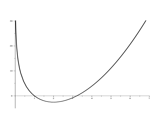
Figure 1: The metric function, Eq. (9), versus $r$ for $\Upsilon=1$, $l=1$, $q=1$ and $M=1$.

which show that they diverge at $r=0$ and are finite for positive $r$. Therefore, one might think that there is an essential singularity located at $r=0$. Since, we are not interested in naked singularity, we look for the existence of horizons and in the other words, we are looking for the possible presence of magnetically charged black hole solutions. As one can see, we will conclude that there are no horizons and thus no black holes. The horizons are given by the zeros of the $g^{rr}$ and so, we investigate the case which $N(r)$ has (at least) one real positive root ($N(r)$ has two real positive roots provided the free parameters of the solution are chosen suitably). Taking into account this case, the function $N(r)$ is negative for $r<r_{+}$, and positive for $r>r_{+}$, where $r_{+}$ is the largest (real) root of $N(r)=0$ (while $N^{\prime}(r_{+})\neq 0$, see Fig. 1). It is worthwhile to note that, $g_{rr}$ and $g_{\psi\psi}$ are related by $N(r)=g_{rr}^{-1}=\Upsilon^{-2}l^{-2}g_{\psi\psi}$, and therefore when $g_{rr}$ becomes negative (which occurs for $0<r<r_{+}$) so $g_{\psi\psi}$ becomes negative too. This fact leads to an apparent change of signature of the metric from $(-,+,+)$ to $(-,-,-)$, and therefore indicates that $r$ should be greater than $r_{+}$. Thus the coordinate $r$ assumes the value $r_{+}\leq r<$ $\infty$. The function $N(r)$ given in Eq. (9) is positive in the whole spacetime and is zero at $r=r_{+}$. In addition, the Kretschmann scalar does not diverge in the range $r_{+}\leq r<\infty$. It is notable that since $\lim_{r\rightarrow r_{+}}\frac{1}{r-r_{+}}\sqrt{\frac{g_{\psi\psi}}{g_{rr}}}\neq 1$, this spacetime may have a conic singularity at $r=r_{+}$, in $(r-\psi)$- section ( the same as discussed in Refs. [20, 22]), and one can remove it by fix the factor $\Upsilon=1/[lN^{\prime}(r_{+})]$ in the metric (and obtain a three dimensional nonsingular horizonless magnetic brane).

2.2 Rotating BTZ magnetic brane

Now, we would like to endow our spacetime solution (3) with a global rotation. At the first step one may think about the mentioned local transformations ($t\longrightarrow il\Upsilon\psi$ and $\psi\longrightarrow it/l$) in the rotating BTZ spacetime [14], $ds^{2}=-N(r)dt^{2}+dr^{2}/N(r)+r^{2}[N^{\phi}dt+d\psi]^{2}$ and obtain

$$ds^{2}=-\frac{r^{2}}{l^{2}}dt^{2}+\frac{dr^{2}}{N(r)}+\Upsilon^{2}l^{2}[N(r)-\left(N^{\phi}\right)^{2}]d\psi^{2}-2N^{\phi}\Upsilon dtd\psi.$$ (12)

Unfortunately, considering Eq. (12) and the field equation (1), lead to complicated differential equations which we could not solve them. In order to add angular momentum to the spacetime, we consider static metric (3) and perform the following rotation boost in the $t-\psi$ plane

$$t\mapsto\Xi t-a\psi,\hskip 14.22636pt\psi\mapsto\Xi\psi-\frac{a}{l^{2}}t,$$ (13)

where $a$ is a rotation parameter and $\Xi=\sqrt{1+a^{2}/l^{2}}$. Substituting Eq. (13) into Eq. (3), we obtain

$$ds^{2}=-\frac{r^{2}}{l^{2}}\left(\Xi dt-ad\psi\right)^{2}+\frac{dr^{2}}{N(r)}+\Upsilon^{2}l^{2}N(r)\left(\frac{a}{l^{2}}dt-\Xi d\psi\right)^{2},$$ (14)

where $N(r)$ is the same as $N(r)$ given in Eq. (9). Since the coordinate $\psi$ is periodic, the transformation (13) is not a proper coordinate transformation on the whole manifold and therefore, the metrics (3) and (14) can be locally mapped into each other but not globally, and so one concludes that they are distinct [23]. In addition, the nonzero components of the gauge potential are $A_{\psi}$ and $A_{t}$

$$A_{\mu}=2ql\Upsilon^{2}h(r)\left(\frac{a}{l}\delta_{\mu}^{t}-\Xi l\delta_{\mu}^{\psi}\right),$$ (15)

Inserting the gauge potential ansatz, Eq. (15), in the electromagnetic field equation (2), surprisingly, leads to Eq. (5) with the same logarithmic form of $h(r)$. Therefore the non-vanishing components of electromagnetic field tensor are now given by

$$F_{tr}=\frac{a}{\Xi l^{2}}F_{r\psi}=\frac{2q\Upsilon^{2}a}{r}.$$ (16)

In this case, one encounters with change of metric signature for $r<r_{+}$ and therefore we should consider this rotating spacetime for $r>r_{+}$. This magnetic solution is both singularity-free and horizon-less in the mentioned interval.

In addition, considering the electromagnetic field tensor given in Eq. (16), one can find that after applying the rotation boost in the $t-\psi$ plane, there appears an electric field ($F_{tr}$). Here, we present a minor physical interpretation for the appearance of the electric field. If we consider that in the static spacetime (observer at rest), there is a static positive charge and a spinning negative charge of equal strength, one may conclude that this system produces no electric field since the total electric charge is zero and the magnetic field is produced by the angular electric current. After applying a rotation boost to a moving observer in the static spacetime, one can show that moving observer can see a different charge density (charge density is a charge over a volume and this volume suffers a Lorentz contraction in the direction of the boost) and a net electric field appears.

3 Generalization to higher dimensional solution:

The higher dimensional action of Einstein gravity which is coupled with a power Maxwell invariant source is given in Refs. [20, 24]. Here, we set power of the Maxwell invariant, $s$, to $n/2$ in the action of ($n+1$)-dimensional Einstein-nonlinear electromagnetic field theory [20, 24]. Using the action principle, one can find the field equations are obtained as

$$R_{\mu\nu}-\frac{1}{2}g_{\mu\nu}(\mathcal{R}-2\Lambda)=\alpha\left(\alpha\mathcal{F}\right)^{n/2-1}\left(\frac{1}{2}g_{\mu\nu}\mathcal{F-}nF_{\mu\lambda}F_{\nu}^{\;\lambda}\right),$$ (17)

$$\partial_{\mu}\left(\sqrt{-g}F^{\mu\nu}\left(\alpha\mathcal{F}\right)^{n/2-1}\right)=0,$$ (18)

where negative cosmological constant, $\Lambda$, is in general equal to $-n(n-1)/2l^{2}$ for asymptotically AdS solutions and $\alpha$ is a constant in which we should fix it.

Here, we want to present an important motivation. It is notable that if we generalize three dimensional charged BTZ solutions to higher dimensional Einstein-Maxwell theory, we encounter with basic changes in the gauge potential and also metric function. In other word, in $(n+1)$-dimensional horizon flat static Reissner–Nordström solutions, the gauge potential and the charge term of the metric function are proportional to $r^{-(n-2)}$ and $r^{-2(n-2)}$, respectively. Therefore, in the 3-dimensional $(n=2)$ case, they reduce to constant values. But for static charged BTZ solutions, the mentioned quantities are proportional to logarithmic function of $r$. Hence, one may conclude that in contrast with the charged BTZ black hole, higher-dimensional Reissner–Nordström solutions reduce to uncharged solutions in three dimensions. Here, we should note that the main goals of this paper are defining the charged magnetic BTZ solution and then generalize our solutions to arbitrary $(n+1)$ dimensions, with wormhole interpretation, in which we will be able to recover charged BTZ solutions, for $n=2$.

3.1 ($n+1$)-dimensional BTZ-like wormhole with a rotation parameter:

Here, we want to obtain the higher dimensional solutions of Eqs. (17), (18) which produce longitudinal magnetic fields. We assume that the metric has the following form

$$ds^{2}=-\frac{r^{2}}{l^{2}}\left(\Xi dt-ad\psi\right)^{2}+\frac{dr^{2}}{N(r)}+\Upsilon^{2}l^{2}N(r)\left(\frac{a}{l^{2}}dt-\Xi d\psi\right)^{2}+r^{2}d\phi^{2}+\frac{r^{2}}{l^{2}}{{\sum_{i=1}^{n-3}}}(dx^{i})^{2}.$$ (19)

Note that the coordinates $-\infty<x^{i}<\infty$ have the dimension of length and the angular coordinates $\psi$ and $\phi$ are dimensionless with the range in $[0,2\pi]$. Also, it is notable that one can obtain the presented metric (19) with local transformations $t\rightarrow il\Upsilon\left(at/l^{2}-\Xi\psi\right)$ and $\psi\rightarrow i\left(\Xi t-a\psi\right)/l$ in the horizon flat Schwarzschild-like metric, $ds^{2}=-N(r)dt^{2}+\frac{dr^{2}}{N(r)}+r^{2}d\psi^{2}+r^{2}d\phi^{2}+\frac{r^{2}}{l^{2}}{{\sum_{i=1}^{n-3}}}(dx^{i})^{2}$. Here we should note that for static case $(a=0)$, third term in Eq. (19) vanishes and (as we will see) we need an angular coordinate such as $\phi$ for construction of wormhole throat at $r=r_{+}$.

Inserting the mentioned gauge potential ansatz, Eq. (15) in the electromagnetic field equation (18) with metric (19), surprisingly, leads to Eq. (5) with logarithmic form for $h(r)$ and the same non-vanishing components of electromagnetic field tensor which presented in Eq. (16).

Now, we should fix the constant $\alpha$ in order to ensure the real solutions. It is easy to show that for a static diagonal magnetic metric ($a=0$) in which the only nonzero component of $A_{\mu}$ is $A_{\psi}$, one can obtain

$$\mathcal{F}=F_{\mu\nu}F^{\mu\nu}=8\left[q\Upsilon lh^{\prime}(r)\right]^{2},$$

and so the power Maxwell invariant, $\left(\alpha\mathcal{F}\right)^{n/2}$, may be imaginary for negative $\alpha$, when $n/2$ is fractional (for even dimensions). Therefore, we set $\alpha=1$, to have real solutions without loss of generality. Setting $\alpha=1$ with $n=2$, it is easy to show that Eqs. (17), (18) reduce to Eqs. (1), (2), as it should be.

To find the metric function $N(r)$, one may use an arbitrary components of Eq. (17) such as $tt$ equation

$$N^{\prime\prime}(r)+2(d-3)\frac{N^{\prime}(r)}{r}+(d-4)(d-3)\frac{N(r)}{r^{2}}-$$

$$\frac{(d-1)(d-2)}{l^{2}}-2^{(d-1)/2}\left(\frac{2ql\Upsilon}{r}\right)^{d-1}=0.$$ (20)

It is easy to find that the solution of Eq. (20) (which satisfy other components of Eq. 17) can be written as

$$N(r)=\frac{r^{2}}{l^{2}}-\frac{1}{r^{d-3}}\left[M+2^{(d-1)/2}\left(2ql\Upsilon\right)^{d-1}\ln\left(\frac{r}{l}\right)\right],$$ (21)

where the integration constant $M$ is related to mass parameter. One should note that these solutions are different from those discussed in [21], which were electrically charged BTZ-like black hole solutions. The electric solutions have BTZ-like black holes, while the magnetic solutions interpret as BTZ-like wormhole.

3.2 Properties of the solutions:

In higher dimensional BTZ-like solutions the Kretschmann and Ricci scalars are

$$R_{\mu\nu\rho\sigma}R^{\mu\nu\rho\sigma} = \frac{(d-1)(d-2)^{2}(d-3)\left[P\ln\left(\frac{r}{l}\right)+M\right]^{2}}{r^{2d-2}}-$$ (22)

$$\frac{2(d-2)(d-3)(2d-3)P\left[P\ln\left(\frac{r}{l}\right)+M\right]}{r^{2d-2}}+$$

$$\frac{(4d^{2}-18d+21)P^{2}}{r^{2d-2}}-\frac{4P}{l^{2}r^{d-1}}+\frac{2d(d-1)}{l^{4}},$$

$$R = \frac{P}{r^{d-1}}-\frac{d(d-1)}{l^{2}},$$ (23)

$$P = 2^{(d-1)/2}\left(2ql\Upsilon\right)^{d-1}$$

which confirm that the presented solutions are asymptotically adS and there is a curvature singularity at $r=0$. Considering $r_{+}$ as largest root of $N(r)=0$ (while $N^{\prime}(r_{+})\neq 0$), we encounter with the same discussion about changing in metric signature for $r<r_{+}$ and so the coordinate $r$ assumes the value $r_{+}\leq r<\infty$. Thus the function $N(r)$ given in Eq. (21) is positive for $r_{+}<r<\infty$. In the same manner, we fix $\Upsilon=1/[lN^{\prime}(r_{+})]$, to avoid conic singularity at $r=r_{+}$ in the $(r-\psi)$-section.

Now, we investigate the wormhole interpretation of the above solution. In order to build static wormhole ($a=0$), we may use the cut-and-paste technique. In this construction, one should take two copies of the solution, Eqs. (19 ) and (21), removing from each copy the forbidden region given by

$$\Omega\equiv\left\{r\mid r<r_{+}\right\}.$$ (24)

With the removal of the forbidden region of each spacetime, we obtain two geodesically incomplete spacetimes with two copies of the following boundaries

$$\partial\Omega\equiv\left\{r\mid r=r_{+}\right\}.$$ (25)

One then identifies the two copies of the mentioned boundaries thereby obtaining a single geodesically complete manifold that contains a wormhole joining the two regions. We can interpret the junction $\partial\Omega$, as the throat of the wormhole. In fact, this wormhole has a throat at $r=r_{+}$.

In order to investigate flare–out condition, we embed the 2-surface of constant $t$, $\psi$ and $x^{i}$’s with the metric $ds^{2}=\frac{dr^{2}}{N(r)}+r^{2}d\phi^{2}$, into an Euclidean flat space of one higher dimension, which has the metric

$$ds^{2}=dr^{2}+r^{2}d\phi^{2}+dz^{2},$$ (26)

The surface described by the function $z=z(r)$ satisfies

$$\frac{dz}{dr}=\left(\left.\sqrt{\frac{N(r)}{1-N(r)}}\right|_{r=r_{+}}\right)^{-1}\longrightarrow\infty,$$ (27)

which shows that the embedded surface is vertical at the throat. Geometrical visualization is not the only use of embedding. Since the throat is a minimum radius from the z-axis, we know that the embedding surface flares outward. Assuming these properties we find that

$$\frac{d^{2}r}{dz^{2}}=\left.\frac{N^{\prime}}{2\left[1-N\right]^{2}}\right|_{r=r_{+}}=\frac{(d-1)r_{+}}{2l^{2}}-\frac{P}{2r_{+}^{d-2}}>0,\text{ for }r_{+}>\left(\frac{Pl^{2}}{d-1}\right)^{1/(d-1)}$$ (28)

which shows that the throat flare out. In other word, the presented charged BTZ wormhole has the characteristic shape of a wormhole, as illustrated in Figs. $1$ and $2$ of Ref. [5].

In order to hold the throat of wormhole open (stable wormhole) there has to be a negative energy density inside. In other word, it is shown that traversable wormholes can exist only if their throats contain exotic matter which possesses a negative pressure and violates the null and weak energy conditions [4, 5, 25, 26]. Violating the energy conditions commits no offense against nature. Although in classical physics the energy density of ordinary forms of matter (fields) is believed to be non-negative [27], it is a well-known fact that energy conditions are violated by certain quantum effects, amongst which we may refer to the squeezed vacuum states in Maxwellian and non-Maxwellian quantum fields, Casimir effect, gravitationally squeezed vacuum zero-point fluctuations, classical scalar fields, the conformal anomaly, gravitational vacuum polarization [26]. So perhaps exotic matter is not utterly impossible. Undoubtedly, the issue of capturing and storing negative energy will be left for future investigations.

Here, we discuss null and weak energy conditions for the BTZ-like in diagonal metric (static case ($a=0$)). Wormholes which could actually be crossed, known as traversable wormholes, would only be possible if exotic matter with negative energy density could be used to stabilize them. For the energy momentum tensor written in the orthonormal contravariant basis vectors as $T^{\mu\nu}=diag(\mu,p_{r},p_{t_{1}},p_{t_{2}},...)$, the mathematics and physical interpretations become simplified (this new basis is the reference frame of a set of observers who remain always at rest in the coordinate system and also $\widehat{g}_{\mu\nu}=\widehat{\eta}_{\mu\nu}$). In new basis vectors, the null energy condition (NEC) holds when $p_{r}+\mu\geq 0$ and $p_{t_{i}}+\mu\geq 0$, and the weak energy condition (WEC) implies $\mu>0$, $p_{r}+\mu\geq 0$ and $p_{t_{i}}+\mu\geq 0$. The physical interpretations of $\mu$, $p_{r}$ and $p_{t_{i}}$’s are, respectively, energy density, radial pressure and tangential pressures that the static observers measure. For diagonal metric, we use the orthonormal contravariant (hatted) basis vectors to simplify interpretation

$$\mathbf{e}_{\widehat{t}}=\frac{l}{r}\frac{\partial}{\partial t},\text{ \ \ }\mathbf{e}_{\widehat{r}}=f^{1/2}\frac{\partial}{\partial r},\text{ \ \ }\mathbf{e}_{\widehat{\psi}}=\frac{1}{\Upsilon lf^{1/2}}\frac{\partial}{\partial\psi},\text{ \ }\mathbf{e}_{\widehat{\phi}}=r^{-1}\frac{\partial}{\partial\phi},\text{ \ }\mathbf{e}_{\widehat{x^{i}}}=\frac{l}{r}\frac{\partial}{\partial x^{i}}.$$

Calculations show that the stress-energy tensor is

$$T_{{}_{\widehat{t}\widehat{t}}} = -T_{{}_{\widehat{\phi}\widehat{\phi}}}=-T_{{}_{\widehat{i}\widehat{i}}}=-2^{(n-2)/2}\left(\frac{F_{r\psi}^{2}}{\Upsilon^{2}l^{2}}\right)^{n/2},$$ (29)

$$\text{ \ \ }T_{{}_{\widehat{r}\widehat{r}}} = T_{{}_{\widehat{\psi}\widehat{\psi}}}=-2^{(n-2)/2}(n-1)\left(\frac{F_{\psi r}^{2}}{\Upsilon^{2}l^{2}}\right)^{n/2},$$ (30)

which one can conclude negative energy density, $T_{{}_{\widehat{t}\widehat{t}}}<0$. This terminology arises because an observer moving through the throat with sufficiently large velocity will necessarily see a negative mass-energy density. In addition, one can confirm the violation of NEC

$$T_{{}_{\widehat{t}\widehat{t}}}+T_{{}_{\widehat{r}\widehat{r}}}=T_{{}_{\widehat{t}\widehat{t}}}+T_{{}_{\widehat{\psi}\widehat{\psi}}}=-2^{(n-2)/2}n\left(\frac{F_{\psi r}^{2}}{\Upsilon^{2}l^{2}}\right)^{n/2}<0.$$ (31)

Indeed, as one expected, wormhole constitutive matter possesses the peculiar property that its stress-energy tensor violates both the NEC and WEC, i.e., we obtain wormhole solutions with exotic matter at the throat.

3.3 Wormhole solutions with more rotation parameters

Now, we can generalize the above solutions to the case of rotating solutions with more than one rotation parameters. We know that the rotation group in $(n+1)-$ dimensions is $SO(n)$ and also the number of (independent) rotation parameters is $[n/2]$ ($[x]$ is the integer part of $x$). The generalized rotating solution with $k\leq[n/2]$ rotation parameters can be written as

$$ds^{2} = -\frac{r^{2}}{l^{2}}\left(\Xi dt-{{\sum_{i=1}^{k}}}a_{i}d\psi^{i}\right)^{2}+\Upsilon^{2}N(r)\left(\sqrt{\Xi^{2}-1}dt-\frac{\Xi}{\sqrt{\Xi^{2}-1}}{{\sum_{i=1}^{k}}}a_{i}d\psi^{i}\right)^{2}$$ (32)

$$+\frac{dr^{2}}{N(r)}+\frac{r^{2}}{l^{2}(\Xi^{2}-1)}{\sum_{i<j}^{k}}(a_{i}d\psi_{j}-a_{j}d\psi_{i})^{2}+r^{2}d\phi^{2}+\frac{r^{2}}{l^{2}}dX^{2},$$

where $\Xi=\sqrt{1+\sum_{i}^{k}a_{i}^{2}/l^{2}}$, $dX^{2}$ is the Euclidean metric on the $(n-k-2)$-dimensional subspace and $N(r)$ is the same as $N(r)$ given in Eq. (21). It is easy to show that the (nonzero) components of electromagnetic field tensor are

$$F_{tr}=\frac{(\Xi^{2}-1)}{\Xi a_{i}}F_{r\psi^{i}}=\frac{2q\Upsilon^{2}l}{r}\sqrt{\Xi^{2}-1}.$$ (33)

Using the same approach, it is worthwhile to note that using these solutions for $r<r_{+}$ lead to an apparent signature change and therefore we should study this spacetime for $r_{+}<r<\infty$. So there are neither horizon nor (curvature) singularity.

3.3.1 Conserved Quantities

Here, we discuss about of the values of the angular momentum, mass density and electrical charge of the solutions. Using the counterterm method [28], we consider the finite energy momentum tensor as

$$T^{ab}=\frac{1}{8\pi}\left[\left(K^{ab}-K\gamma^{ab}\right)-\left(\frac{n-1}{l}\right)\gamma^{ab}\right],$$ (34)

where $K^{ab}$ is the extrinsic curvature (of the boundary), $K$ is its trace, $\gamma^{ab}$ is the induced metric (of the boundary). To compute the conserved charges of the spacetime, we can follow the procedure which presented in [20, 22]. The first Killing vector is $\xi=\partial/\partial t$ which is related to the total mass of the wormhole per unit volume $V_{n-k-1}$, given by

$$M=\frac{(2\pi)^{k}}{4}\left[n(\Xi^{2}-1)+1\right]\Upsilon m.$$ (35)

For the rotating case, the other killing vectors are $\zeta_{i}=\partial/\partial\phi^{i}$ which are related to the components of angular momentum per unit volume $V_{n-k-1}$ calculated as

$$J_{i}=\frac{(2\pi)^{k}}{4}n\Upsilon\Xi ma_{i},$$ (36)

which confirms that $a_{i}$’s are rotation parameters. At final step, we should calculate the electric charge per unit volume $V_{n-k-1}$ of the solutions. In order to calculate it one can take into account the projections of the electromagnetic field tensor and obtan the flux of the electromagnetic field at infinity, yielding

$$Q=\frac{(2\pi)^{k}2^{3n/2}n\Upsilon\left(\frac{q}{l}\right)^{n-1}}{16}\sqrt{\Xi^{2}-1}.$$ (37)

It is worth noticing that the electric charge of the wormhole per unit volume $V_{n-k-1}$ is proportional to the rotation parameters, and is zero for the static wormhole solutions ($\Xi=1$). This result is expected since now, besides the magnetic field along the $\psi$ coordinate, there is also a radial electric field ($F_{tr}\neq 0$) and the former component leads to an electric charge.

4 Closing Remarks

In this paper, we have demonstrated a construction $n+1$-dimensional magnetically charged solutions, namely charged BTZ-like wormholes. Considering three dimensional magnetic solution of Einstein-Maxwell gravity, we obtained a static charged BTZ magnetic brane. We found that the Kretschmann scalar is finite in whole spacetime and there is no horizon. Then, we used an improper coordinate transformation to add an angular momentum in the magnetic brane.

After that, we generalized our solutions to arbitrary $(n+1)$ dimensions in which, in contrast with higher dimensional Reissner–Nordström solutions, we were able to recover BTZ solutions, for $n=2$. We also checked the flare-out condition and found that charged BTZ-like solutions satisfied the flare-out condition (with wormhole interpretation) provided the free parameters of the solution are chosen suitably. In addition, calculation of energy conditions showed that charged BTZ-like wormholes supported by an exotic matter at their throats ($r=r_{+}$).

Finally, we generalized charged BTZ-like wormhole solutions to the case of rotating solutions with more rotation parameters and calculated some conserved quantities such as angular momentum and mass density. Also, we analyzed the flux of the electromagnetic field at infinity for the BTZ-like solutions and found that the electric charge density of the charged BTZ-like wormholes depends on the magnitude of the rotation parameters, while the static charged BTZ-like wormholes have no net electric charge.

We should note that it is worthwhile to investigate the dynamic stability of the charged BTZ-like wormhole solutions with respect to radial perturbations.

References

- [1] A. Einstein and N. Rosen, Phys. Rev. 48, 73 (1935).
- [2] J. A. Wheeler, Phys. Rev. 97, 511 (1955).
- [3] R. W. Fuller and J. A. Wheeler, Phys. Rev. 128, 919 (1962).
- [4] H. G. Ellis, J. Math. Phys. 14, 395 (1973); G. Clement, Am. J. Phys. 57, 967 (1989).
- [5] M. S. Morris and K. S. Thorne, Am. J. Phys. 56, 395 (1988); M. S. Morris, K. S. Thorne and U. Yurtsever, Phys. Rev. Lett. 61, 1446 (1988); L. H. Ford and T. A. Roman, Phys. Rev. D 51, 4277 (1995); K. D. Olum, Phys. Rev. Lett. 81, 3567 (1998); V. Sopova and L. H. Ford, Phys. Rev. D 66, 045026 (2002).
- [6] E. Gravanis and S. Willison, Phys. Rev. D 75, 084025 (2007).
- [7] M. H. Dehghani and S. H. Hendi, Gen. Relativ. Gravit. 41, 1853 (2009).
- [8] S. H. Hendi, Can. J. Phys. 89, 281 (2011); S. H. Hendi, J. Math. Phys. 52, 042502 (2011).
- [9] E. Witten, Adv. Theor. Math. Phys. 2, 505 (1998).
- [10] S. Carlip, Class. Quantum Gravit. 12, 2853 (1995).
- [11] A. Ashtekar, Adv. Theor. Math. Phys. 6, 507 (2002).
- [12] T. Sarkar, G. Sengupta, B. Nath Tiwari, JHEP. 0611, 015 (2006).
- [13] E. Witten, [arXiv:0706.3359].
- [14] M. Banados, C. Teitelboim and J. Zanelli, Phys. Rev. Lett. 69, 1849(1992).
- [15] M. Banados, M. Henneaux, C. Teitelboim and J. Zanelli, Phys. Rev. D 48, 1506 (1993).
- [16] S. Nojiri and S. D. Odintsov, Mod. Phys. Lett. A 13, 2695 (1998); R. Emparan, G. T. Horowitz and R. C. Myers, JHEP 0001, 021 (2000); S. Hemming, E. Keski-Vakkuri and P. Kraus, JHEP 0210, 006 (2002); M. R. Setare, Class. Quantum Gravit. 21, 1453 (2004); B. Sahoo and A. Sen, JHEP 0607, 008 (2006); M. R. Setare, Eur. Phys. J. C 49, 865 (2007); M. Cadoni and M. R. Setare, JHEP 0807, 131 (2008); M. Park, Phys. Rev. D 77, 026011 (2008); M. Park, Phys. Rev. D 77, 126012 (2008); J. Parsons and S. F. Ross, JHEP 0904, 134 (2009); M. R. Setare and M. Jamil, Phys. Lett. B 681, 469 (2009).
- [17] S. Carlip, Class. Quantum Gravit. 22, R85 (2005).
- [18] S. Aminneborg and et al., Class. Quantum Gravit. 15, 627 (1998); D. Brill, [arXiv:gr-qc/9904083]; S. Holst and H. J. Matschull, Class. Quantum Gravit. 16, 3095 (1999); W. T. Kim, J. J. Oh and M. S. Yoon, Phys. Rev. D 70, 044006 (2004); A. Larranaga, Rev. Col. Fis. 40, 222 (2008); M. U. Farooq, M. Akbar and M. Jamil, AIP Conf. Proc. 1295, 176 (2010); F. Rahaman, A. Banerjee and I Radinschi, [arXiv:1109.0976].
- [19] O. J. C. Dias and J. P. S. Lemos, Class. Quantum Gravit. 19, 2265 (2002); O. J. C. Dias and J. P. S. Lemos, JHEP 0201, 006 (2002); G. A. S. Dias and J. P. S. Lemos, [arXiv:1008.3376]; M. H. Dehghani, N. Bostani and S. H. Hendi, Phys. Rev. D 78, 064031 (2008); M. H. Dehghani, A. Sheykhi and S. H. Hendi, Phys. Lett. B 659, 476 (2008).
- [20] S. H. Hendi, Class. Quantum Gravit. 26, 225014 (2009).
- [21] S. H. Hendi, Eur. Phys. J. C 71, 1551 (2011).
- [22] S. H. Hendi, S. Kordestani and S. N. D. Motlagh, Prog. Theor. Phys. 124, 1067 (2010).
- [23] J. Stachel, Phys. Rev. D 26, 1281 (1982).
- [24] M. Hassaine and C. Martinez, Class. Quantum Gravit. 25, 195023 (2008); S. H. Hendi, Phys. Lett. B 678, 438 (2009); S. H. Hendi, Phys. Lett. B 690, 220 (2010); S. H. Hendi and B. Eslam Panah, Phys. Lett. B 684, 77 (2010); S. H. Hendi, Eur. Phys. J. C 69, 281 (2010); S. H. Hendi, Prog. Theor. Phys. 124, 493 (2010); S. H. Hendi, Phys. Rev D 82, 064040 (2010).
- [25] D. Hochberg and M. Visser, Phys. Rev. D 56, 4745 (1997); D. Hochberg and M. Visser, Phys. Rev. D 58, 044021 (1998).
- [26] H. Epstein, V. Glaser, and A. Jaffe, Nuovo Cim. 36, 1016 (1965); H. B. G. Casimir, Proc. Kon. Ned. Akad. Wetensch. B 51, 793 (1948); S. Lamoreaux, Phys. Rev. Lett. 78, 5 (1996); U. Mohideen and A. Roy, Phys. Rev. Lett. 81, 4549 (1998); M. Visser, Phys. Rev. D 54, 5103 (1996); M. Visser, Phys. Rev. D 54, 5116 (1996); M. Visser, Phys. Rev. D 54, 5123 (1996); M. Visser, Phys. Rev. D 56, 936 (1997); M. Visser, [Arxiv:gr-qc/9710034]; C. Barcelo and M. Visser, Int. J. Mod. Phys. D 11, 1553 (2002); D. Hochberg, A. Popov and S. V. Sushkov, Phys. Rev. Lett. 78, 2050 (1997); S. H. Hendi and D. Momeni, Eur. Phys. J. C 71, 1823 (2011).
- [27] S. W. Hawking and G. F. R. Ellis, The Large Scale Structure of Spacetime, (Cambridge University Press, Cambridge 1973).
- [28] J. Maldacena, Adv. Theor. Math. Phys. 2, 231 (1998); E. Witten, Adv. Theor. Math. Phys. 2, 253 (1998); O. Aharony, S. S. Gubser, J. Maldacena, H. Ooguri and Y. Oz, Phys. Rept. 323, 183 (2000).