Efficient computational noise in GLSL

Abstract

We present GLSL implementations of Perlin noise and Perlin simplex noise that run fast enough for practical consideration on current generation GPU hardware. The key benefits are that the functions are purely computational, i.e. they use neither textures nor lookup tables, and that they are implemented in GLSL version 1.20, which means they are compatible with all current GLSL-capable platforms, including OpenGL ES 2.0 and WebGL 1.0. Their performance is on par with previously presented GPU implementations of noise, they are very convenient to use, and they scale well with increasing parallelism in present and upcoming GPU architectures.

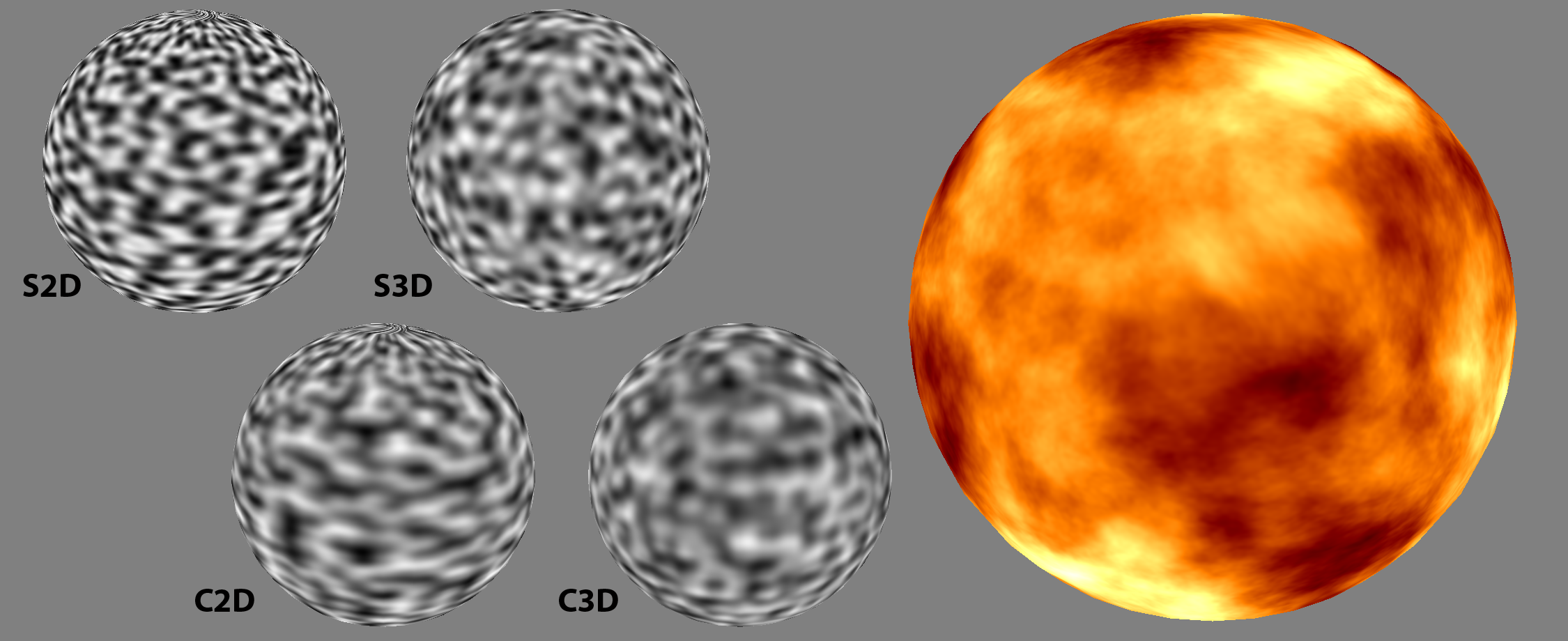
Figure 1: 2D and 3D simplex noise (S2D, S3D) and 2D and 3D classic noise (C2D, C3D) on a sphere, and a swirling fire shader using several noise components.

1 Introduction and background

Perlin noise [1, 3] is one of the most useful building blocks of procedural shading in software. The natural world is largely built on or from stochastic processes, and manipulation of noise allows a variety of natural materials and environments to be procedurally created with high flexibility, at minimal labor and at very modest computational costs. The introduction of Perlin Noise revolutionized the offline rendering of artificially-created worlds.

Hardware shading has not yet adopted procedural methods to any significant extent, because of limited GPU performance and strong real time constraints. However, with the recent rapid increase in GPU parallelism and performance, texture memory bandwidth is often a bottleneck, and procedural patterns are becoming an attractive alternative and a complement to traditional image-based textures.

Simplex noise [2] is a variation on classic Perlin noise, with the same general look but with a different computational structure. The benefits include a lower computational cost for high dimensional noise fields, a simple analytic derivative, and an absence of axis-aligned artifacts. Simplex noise is a gradient lattice noise just like classic Perlin noise and uses the same fundamental building blocks. Some examples of noise on a sphere are shown in Figure 1.

This presentation assumes the reader is familiar with classic Perlin noise and Perlin simplex noise. A summary of both is presented in [6]. We will focus on how our approach differs from software implementations and from the previous GLSL implementations in [4, 5].

2 Platform constraints

GLSL 1.20 implementations usually do not allow dynamic access of arrays in fragment shaders, lack support for 3D textures and integer texture lookups, have no integer logic operations, and don’t optimize conditional code well. Previous noise implementations rely on many of these features, which limits their use on these platforms. Integer table lookups implemented by awkward floating point texture lookups produces unnecessarily slow and complex code and consumes texture resources. Supporting code outside of the fragment shader is needed to generate these tables or textures, preventing a concise, encapsulated, reusable GLSL implementation independent of the application environment. Our solutions to these problems are:

• Replace permutation tables with computed permutation polynomials.

• Use computed points on a cross polytope surface to select gradients.

• Replace conditionals for simplex selection with rank ordering.

These concepts are explained below. The resulting noise functions are completely self contained, with no references to external data and requiring only a few registers of temporary storage.

3 Permutation polynomials

Previously published noise implementations have used permutation tables or bit-twiddling hashes to generate pseudo-random gradient indices. Both of these approaches are unsuitable for our purposes, but there is another way. A permutation polynomial is a function that uniquely permutes a sequence of integers under modulo arithmetic, in the same sense that a permutation lookup table is a function that uniquely permutes a sequence of indices. A more thorough explanation of permutation polynomials can be found in the online supplementary material to this article. Here, we will only point out that useful permutations can be constructed using polynomials of the simple form $(Ax^{2}+Bx)\bmod{M}$. For example, The integers modulo-9 admit the permutation polynomial $(6x^{2}+x)\bmod{9}$ giving the permutation $(0\ 1\ 2\ 3\ 4\ 5\ 6\ 7\ 8)\mapsto(0\ 7\ 8\ 3\ 1\ 2\ 6\ 4\ 5)$.

The number of possible polynomial permutations is a small subset of all possible shufflings, but there are more than enough of them for our purposes. We need only one that creates a good shuffling of a few hundred numbers, and the particular one we chose for our implementation is $(34x^{2}+x)\bmod{289}$.

What is more troublesome is the often inadequate integer support in GLSL 1.20 that effectively forces us to use single precision floats to represent integers. There are only 24 bits of precision to play with (counting the implicit leading 1), and a floating point multiplication doesn’t drop the highest bits on overflow. Instead it loses precision by dropping the low bits that do not fit and adjusts the exponent. This would be fatal to a permutation algorithm, where the least significant bit is essential and must not be truncated in any operation. If the computation of our chosen polynomial is implemented in the straightforward manner, truncation occurs when $34x^{2}+x>2^{24}$, or $|x|>702$ in the integer domain. If we instead observe that modulo-$M$ arithmetic is congruent for modulo-$M$ operation on any operand at any time, we can start by mapping $x$ to $x\bmod{289}$ and then compute the polynomial $34x^{2}+x$ without any risk for overflow. By this modification, truncation does not occur for any $x$ that can be exactly represented as a single precision float, and the noise domain is instead limited by the remaining fractional part precision for the input coordinates. Any single precision implementation of Perlin noise, in hardware or software, shares this limitation.

4 Gradients on $N$-cross-polytopes

Lattice gradient noise associates pseudo-random gradients with each lattice point. Previous implementations have used pre-computed lookup tables or bit manipulations for this purpose. We use a more floating-point friendly way and make use of geometric relationships between generalized octahedrons in different numbers of dimensions to map evenly distributed points from an ($N$-1)-dimensional cube onto the boundary of the $N$-dimensional equivalent of an octahedron, an $N$-cross polytope. For $N=2$, points on a line segment are mapped to the perimeter of a rotated square, see Figure 2. For $N=3$, points in a square map to an octahedron, see Figure 3, and for $N=4$, points in a cube are mapped to the boundary of a 4-D truncated cross polytope. Equation (1) presents the mappings for the 2-D, 3-D and 4-D cases.

2-D: $$x_{0}\in[-2,2],\quad y=1-|x_{0}|$$ (1)

$$\textbf{if~{}}y>0\textbf{~{}then~{}}x=x_{0}\textbf{~{}else~{}}x=x_{0}-\text{sign}(x_{0})$$

3-D: $$x_{0},y_{0}\in[-1,1],\quad z=1-|x_{0}|-|y_{0}|$$

$$\textbf{if~{}}z>0\textbf{~{}then~{}}x=x_{0},~{}y=y_{0}$$

$$\textbf{~{}else~{}}x=x_{0}-\text{sign}(x_{0}),~{}y=y_{0}-\text{sign}(y_{0})$$

4-D: $$x_{0},y_{0},z_{0}\in[-1,1],\quad w=1.5-|x_{0}|-|y_{0}|-|z_{0}|$$

$$\textbf{if~{}}w>0\textbf{~{}then~{}}x=x_{0},~{}y=y_{0},~{}z=z_{0}$$

$$\textbf{~{}else~{}}x=x_{0}-\text{sign}(x_{0}),~{}y=y_{0}-\text{sign}(y_{0}),~{}z=z_{0}-\text{sign}(z_{0})$$

The mapping for the 4-D case doesn’t cover the full polytope boundary – it truncates six of the eight corners slightly. However, the mapping covers enough of the boundary to yield a visually isotropic noise field, and it is a simple mapping. The 4-D mapping is difficult both to understand and to visualize, but it is explained in more detail in the supplementary material.

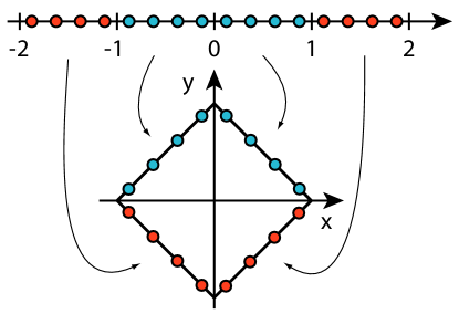
Figure 2: Mapping from a 1-D line segment to the boundary of a 2-D diamond shape.

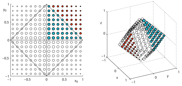
Figure 3: Mapping from a 2-D square to the boundary of a 3-D octahedron. Blue points in the quadrant $x>0,y>0$ where $|x|+|y|<1$ map to the face $x,y,z>0$, while red points where $|x|+|y|>1$ map to the opposite face $x,y,z<0$.

Most implementations of Perlin noise use gradient vectors of equal length, but the longest and shortest vectors on the surface of an $N$-dimensional cross polytope differ in length by a factor of $\sqrt{N}$. This does not cause any strong artifacts, because the generated pattern is irregular anyway, but for higher dimensional noise the pattern becomes less isotropic if the vectors are not explicitly normalized. Normalization needs only to be performed in an approximate fashion, so we use the linear part of a Taylor expansion for the inverse square root $1/\sqrt{r}$ in the neighborhood of $r=0.7$. The built-in GLSL function inversesqrt() is likely to be just as fast on most platforms. Normalization can even be skipped entirely for a slight performance gain.

5 Rank ordering

Simplex noise uses a two step process to determine which simplex contains a point $\mathbf{p}$. First, the N-simplex grid is transformed to an axis-aligned grid of $N$-cubes, each containing $N!$ simplices. The determination of which cube contains $\mathbf{p}$ only requires computing the integer part of the transformed coordinates. Then, the coordinates relative to the origin of the cube are computed by inverse transforming the fractional part of the transformed coordinates, and a rank ordering is used to determine which simplex contains $x$. Rank ordering is the first stage of the unusual but classic rank sorting algorithm, where the values are first ranked and then rearranged into their sorted order. Rank ordering can be performed efficiently by pair-wise comparisons of components of $\mathbf{p}$. Two components can be ranked by a single comparison, three components by three comparisons and four components can be ranked by six comparisons. In GLSL, up to four comparisons can be performed in parallel using vector operations. The ranking can be determined in a reasonably straightforward manner from the results of these comparisons. The rank ordering approach was used in a roundabout way in the software 4D noise implementation of [6] and the GLSL implementation of [5], later improved and generalized by contributions from Bill Licea-Kane at AMD (then ATI). The 3D noise of [6] and Perlin’s original software implementation presented in [2] instead use a decision tree of conditionals. For details on the rank ordering algorithm used for 3-D and 4-D simplex noise, which generalizes to $N$-D, we refer to the supplementary material.

6 Performance and source code

The performance of the presented algorithms is good, as presented in Table 1. With reasonably recent GPU hardware, 2-D noise runs at a speed of several billion samples per second. 3-D noise attains about half that speed, and 4-D noise is somewhat slower still, with a clear speed advantage for 3-D and 4-D simplex noise compared to classic noise. All variants are fast enough to be considered for practical use on current GPU hardware.

Procedural texturing scales better than traditional texturing with massive amounts of parallel execution units, because it is not dependent on texture bandwidth. Looking at recent generations of GPUs, parallelism seems to increase more rapidly in GPUs than texture bandwidth. Also, embedded GPU architectures designed for OpenGL ES 2.x have limited texture resources and may benefit from procedural noise despite their relatively low performance.

The full GLSL source code for 2D simplex noise is quite compact, as presented in Table 3. For the gradient mapping, this particular implementation wraps the integer range $\{0\ldots 288\}$ repeatedly to the range $\{0\ldots 40\}$ by a modulo-41 operation. 41 has no common prime factors with 289, which improves the shuffling, and 41 is reasonably close to an even divisor of 289, which creates a good isotropic distribution for the gradients.

Counting vector operations as a single operation, this code amounts to just six dot operations, three mod, two floor, one each of step, max, fract and abs, seventeen multiplications and nineteen additions. The supplementary material contains source code for 2-D, 3-D and 4-D simplex noise, classic Perlin noise and a periodic version of classic noise with an explicitly specified arbitrary integer period, to match the popular and useful pnoise() function in RenderMan SL. The source code is licensed under the MIT license. Attribution is required where substantial portions of the work is used, but there are no other limits on commercial use or modifications. Managed and tracked code and a cross-platform benchmark and demo for Linux, MacOS X and Windows can be downloaded from the public git repository git@github.com:ashima/webgl-noise.git, reachable also by:
http://www.github.com/ashima/webgl-noise

	Const	Simplex noise			Classic noise
GPU	color	2D	3D	4D	2D	3D	4D
Nvidia
GF7600GS	3,399	162	72	39	180	43	16
GTX260	8,438	1,487	784	426	1,477	589	255
GTX480	8,841	3,584	1,902	1,149	3,489	1,508	681
GTX580	13,863	4,676	2,415	1,429	4,675	2,003	906
AMD
HD3650	1,974	370	193	117	320	147	67
HD4850	9,416	2,586	1,320	821	2,142	992	457
HD5870	18,061	4,980	3,062	2,006	4,688	2,211	1,092

Table 1: Performance benchmarks for selected GPUs, in Msamples per second

7 Old versus new

The described noise implementations are fundamentally different from previous work, in that they use no lookup tables at all. The advantage is that they scale very well with massive parallelism and are not dependent on texture memory bandwidth. The lack of lookup tables makes them suitable for a VLSI hardware implementation in silicon, and they can be used in vertex shader environments where texture lookup is not guaranteed to be available, as in the baseline OpenGL ES 2.0 and WebGL 1.0 profiles.

In terms of performance, this purely computational noise is not quite as fast on current GPUs as the previous implementation by Gustavson [5], which made heavy use of 2-D texture lookups both for permutations and gradient generation. Most real time graphics of today is very texture intensive, and modern GPU architectures are designed to have a high texture bandwidth. However, it should be noted that noise is mostly just one component of a shader, and a computational noise algorithm can make good use of unutilised ALU resources in an otherwise texture intensive shader. Furthermore, we consider the simplicity that comes from independence of external data to be an advantage in itself.

A side by side comparison of the new implementation against the previous implementation is presented in Table 2. The old implementation is roughly twice as fast as our purely computational version, although the gap appears to be closing with more recent GPU models with better computing power. It is worth noting that 4D classic noise needs 16 pseudo-random gradients, which requires 64 simple quadratic polynomial evaluations and 16 gradient mappings in our new implementation, and a total of 48 2-D texture lookups in the previous implementation. The fact that the old version is faster despite its very heavy use of texture lookups shows that current GPUs are very clearly designed for streamlining texture memory accesses.

8 Supplementary material

http://www.itn.liu.se/~stegu/jgt2011/supplement.pdf

	Const	Simplex noise			Classic noise
GPU, version	color	2D	3D	4D	2D	3D	4D
Nvidia
GTX260 new	8,438	1,487	784	426	1,477	589	255
GTX260 old		2,617	1,607	953	3,367	1,815	921
GTX580 new	13,863	4,676	2,415	1,429	4,675	2,003	906
GTX580 old		7,806	4,481	2,692	8,795	3,508	1,869
AMD
HD3650 new	1,974	370	193	117	320	147	67
HD3650 old		665	413	241	871	333	139
HD4850 new	9,416	2,586	1,320	821	2,142	992	457
HD4850 old		4,615	2,874	1,524	5,654	1,926	956

Table 2: Performance of old vs. new implementation, in Msamples per second.

⬇

[rgb]0.133,0.545,0.133// 2D simplex noise

#version 120

[rgb]0,0,1vec3 permute([rgb]0,0,1vec3 x) {

[rgb]0,0,1return [rgb]0,0,1mod(((x*34.0)+1.0)*x, 289.0); }

[rgb]0,0,1vec3 taylorInvSqrt([rgb]0,0,1vec3 r) {

[rgb]0,0,1return 1.79284291400159 - 0.85373472095314 * r; }

[rgb]0,0,1float snoise([rgb]0,0,1vec2 P) {

const [rgb]0,0,1vec2 C = [rgb]0,0,1vec2(0.211324865405187134, [rgb]0.133,0.545,0.133// (3.0-sqrt(3.0))/6.0;

0.366025403784438597); [rgb]0.133,0.545,0.133// 0.5*(sqrt(3.0)-1.0);

[rgb]0.133,0.545,0.133// First corner

[rgb]0,0,1vec2 i = [rgb]0,0,1floor(P + [rgb]0,0,1dot(P, C.yy) );

[rgb]0,0,1vec2 x0 = P - i + [rgb]0,0,1dot(i, C.xx);

[rgb]0.133,0.545,0.133// Other corners

[rgb]0,0,1vec2 i1;

i1.x = [rgb]0,0,1step( x0.y, x0.x ); [rgb]0.133,0.545,0.133// 1.0 if x0.x > x0.y, else 0.0

i1.y = 1.0 - i1.x;

[rgb]0.133,0.545,0.133// x1 = x0 - i1 + 1.0 * C.xx; x2 = x0 - 1.0 + 2.0 * C.xx;

[rgb]0,0,1vec4 x12 = x0.xyxy + [rgb]0,0,1vec4( C.xx, C.xx * 2.0 - 1.0);

x12.xy -= i1;

[rgb]0.133,0.545,0.133// Permutations

i = [rgb]0,0,1mod(i, 289.0); [rgb]0.133,0.545,0.133// Avoid truncation in polynomial evaluation

[rgb]0,0,1vec3 p = permute( permute( i.y + [rgb]0,0,1vec3(0.0, i1.y, 1.0 ))

+ i.x + [rgb]0,0,1vec3(0.0, i1.x, 1.0 ));

[rgb]0.133,0.545,0.133// Circularly symmetric blending kernel

[rgb]0,0,1vec3 m = [rgb]0,0,1max(0.5 - [rgb]0,0,1vec3([rgb]0,0,1dot(x0,x0), [rgb]0,0,1dot(x12.xy,x12.xy),

[rgb]0,0,1dot(x12.zw,x12.zw)), 0.0);

m = m*m;

m = m*m;

[rgb]0.133,0.545,0.133// Gradients from 41 points on a line, mapped onto a diamond

[rgb]0,0,1vec3 x = [rgb]0,0,1fract(p * (1.0 / 41.0)) * 2.0 - 1.0 ;

[rgb]0,0,1vec3 gy = [rgb]0,0,1abs(x) - 0.5 ;

[rgb]0,0,1vec3 ox = [rgb]0,0,1floor(x + 0.5); [rgb]0.133,0.545,0.133// round(x) is a GLSL 1.30 feature

[rgb]0,0,1vec3 gx = x - ox;

[rgb]0.133,0.545,0.133// Normalise gradients implicitly by scaling m

m *= taylorInvSqrt( gx*gx + gy*gy );

[rgb]0.133,0.545,0.133// Compute final noise value at P

[rgb]0,0,1vec3 g;

g.x = gx.x * x0.x + gy.x * x0.y;

g.yz = gx.yz * x12.xz + gy.yz * x12.yw;

[rgb]0.133,0.545,0.133// Scale output to span range [-1,1]

[rgb]0.133,0.545,0.133// (scaling factor determined by experiments)

[rgb]0,0,1return 130.0 * [rgb]0,0,1dot(m, g);

}

Table 3: Complete, self-contained source code for 2D simplex noise. Code for 2D, 3D and 4D versions of classic and simplex noise is in the supplementary material and in the online repository.

Ian McEwan, David Sheets and Mark Richardson, Ashima Research, 600 S. Lake Ave., Suite 104, Pasadena CA 91106, USA
(ijm@ashimaresearch.com, sheets@ashimaresearch.com, mir@ashimaresearch.com)

Stefan Gustavson, Media and Information Technology, ITN, Linköping University, 60174 Norrköping, Sweden
(stefan.gustavson@liu.se)

Received [DATE]; accepted [DATE].

References

- [1] Ken Perlin, An Image Synthesizer. Computer Graphics (Proceedings of ACM SIGGRAPH 85), Vol. 19, Number 3, pp. 287–296, 1985.
- [2] Ken Perlin, Noise Hardware. SIGGRAPH 2001 course notes, Vol. 24 (Real-Time Shading), Chapter 9, 2001.
- [3] Ken Perlin, Improving Noise, ACM Transactions on Graphics (Proceedings of SIGGRAPH 2002) Vol. 21, Number 3, pp 681–682, 2002.
- [4] Simon Green, Implementing Improved Perlin Noise. GPU Gems 2, Chapter 26, Addison-Wesley, 2005.
- [5] Stefan Gustavson, Perlin noise implementation in GLSL. Post to the GLSL developer forum at www.opengl.org, November 24, 2004.
-
[6]