EUROPEAN ORGANIZATION FOR NUCLEAR RESEARCH (CERN)

​​​ CERN-PH-EP-2012-068 LHCb-PAPER-2011-030

Measurement of the ratio of prompt $\chi_{c}$ to ${J\mskip-3.0mu/\mskip-2.0mu\psi\mskip 2.0mu}$ production in $pp$ collisions at $\sqrt{s}\,{=}\,\mbox{${7}\>{\mathrm{\,Te\kern-2.07413ptV}}$}$

The LHCb collaboration

The prompt production of charmonium $\chi_{c}$ and $J/\psi$ states is studied in proton-proton collisions at a centre-of-mass energy of $\sqrt{s}=7$ TeV at the Large Hadron Collider. The $\chi_{c}$ and $J/\psi$ mesons are identified through their decays $\chi_{c}\rightarrow J/\psi\gamma$ and $J/\psi\rightarrow\mu^{+}\mu^{-}$ using 36 pb^-1 of data collected by the LHCb detector in 2010. The ratio of the prompt production cross-sections for $\chi_{c}$ and $J/\psi$, $\sigma(\chi_{c}\rightarrow J/\psi\gamma)/\sigma(J/\psi)$, is determined as a function of the $J/\psi$ transverse momentum in the range $2<p_{\mathrm{T}}^{J/\psi}<15$ GeV/$c$. The results are in excellent agreement with next-to-leading order non-relativistic expectations and show a significant discrepancy compared with the colour singlet model prediction at leading order, especially in the low $p_{\mathrm{T}}^{J/\psi}$ region.

Submitted to Phys. Lett. B

 

LHCb collaboration

R. Aaij³⁸, C. Abellan Beteta^33,n, B. Adeva³⁴, M. Adinolfi⁴³, C. Adrover⁶, A. Affolder⁴⁹, Z. Ajaltouni⁵, J. Albrecht³⁵, F. Alessio³⁵, M. Alexander⁴⁸, S. Ali³⁸, G. Alkhazov²⁷, P. Alvarez Cartelle³⁴, A.A. Alves Jr²², S. Amato², Y. Amhis³⁶, J. Anderson³⁷, R.B. Appleby⁵¹, O. Aquines Gutierrez¹⁰, F. Archilli^18,35, L. Arrabito⁵⁵, A. Artamonov ³², M. Artuso^53,35, E. Aslanides⁶, G. Auriemma^22,m, S. Bachmann¹¹, J.J. Back⁴⁵, V. Balagura^28,35, W. Baldini¹⁶, R.J. Barlow⁵¹, C. Barschel³⁵, S. Barsuk⁷, W. Barter⁴⁴, A. Bates⁴⁸, C. Bauer¹⁰, Th. Bauer³⁸, A. Bay³⁶, I. Bediaga¹, S. Belogurov²⁸, K. Belous³², I. Belyaev²⁸, E. Ben-Haim⁸, M. Benayoun⁸, G. Bencivenni¹⁸, S. Benson⁴⁷, J. Benton⁴³, R. Bernet³⁷, M.-O. Bettler¹⁷, M. van Beuzekom³⁸, A. Bien¹¹, S. Bifani¹², T. Bird⁵¹, A. Bizzeti^17,h, P.M. Bjørnstad⁵¹, T. Blake³⁵, F. Blanc³⁶, C. Blanks⁵⁰, J. Blouw¹¹, S. Blusk⁵³, A. Bobrov³¹, V. Bocci²², A. Bondar³¹, N. Bondar²⁷, W. Bonivento¹⁵, S. Borghi^48,51, A. Borgia⁵³, T.J.V. Bowcock⁴⁹, C. Bozzi¹⁶, T. Brambach⁹, J. van den Brand³⁹, J. Bressieux³⁶, D. Brett⁵¹, M. Britsch¹⁰, T. Britton⁵³, N.H. Brook⁴³, H. Brown⁴⁹, K. de Bruyn³⁸, A. Büchler-Germann³⁷, I. Burducea²⁶, A. Bursche³⁷, J. Buytaert³⁵, S. Cadeddu¹⁵, O. Callot⁷, M. Calvi^20,j, M. Calvo Gomez^33,n, A. Camboni³³, P. Campana^18,35, A. Carbone¹⁴, G. Carboni^21,k, R. Cardinale^19,i,35, A. Cardini¹⁵, L. Carson⁵⁰, K. Carvalho Akiba², G. Casse⁴⁹, M. Cattaneo³⁵, Ch. Cauet⁹, M. Charles⁵², Ph. Charpentier³⁵, N. Chiapolini³⁷, K. Ciba³⁵, X. Cid Vidal³⁴, G. Ciezarek⁵⁰, P.E.L. Clarke^47,35, M. Clemencic³⁵, H.V. Cliff⁴⁴, J. Closier³⁵, C. Coca²⁶, V. Coco³⁸, J. Cogan⁶, P. Collins³⁵, A. Comerma-Montells³³, A. Contu⁵², A. Cook⁴³, M. Coombes⁴³, G. Corti³⁵, B. Couturier³⁵, G.A. Cowan³⁶, R. Currie⁴⁷, C. D’Ambrosio³⁵, P. David⁸, P.N.Y. David³⁸, I. De Bonis⁴, S. De Capua^21,k, M. De Cian³⁷, F. De Lorenzi¹², J.M. De Miranda¹, L. De Paula², P. De Simone¹⁸, D. Decamp⁴, M. Deckenhoff⁹, H. Degaudenzi^36,35, L. Del Buono⁸, C. Deplano¹⁵, D. Derkach^14,35, O. Deschamps⁵, F. Dettori³⁹, J. Dickens⁴⁴, H. Dijkstra³⁵, P. Diniz Batista¹, F. Domingo Bonal^33,n, S. Donleavy⁴⁹, F. Dordei¹¹, A. Dosil Suárez³⁴, D. Dossett⁴⁵, A. Dovbnya⁴⁰, F. Dupertuis³⁶, R. Dzhelyadin³², A. Dziurda²³, S. Easo⁴⁶, U. Egede⁵⁰, V. Egorychev²⁸, S. Eidelman³¹, D. van Eijk³⁸, F. Eisele¹¹, S. Eisenhardt⁴⁷, R. Ekelhof⁹, L. Eklund⁴⁸, Ch. Elsasser³⁷, D. Elsby⁴², D. Esperante Pereira³⁴, A. Falabella^16,e,14, C. Färber¹¹, G. Fardell⁴⁷, C. Farinelli³⁸, S. Farry¹², V. Fave³⁶, V. Fernandez Albor³⁴, M. Ferro-Luzzi³⁵, S. Filippov³⁰, C. Fitzpatrick⁴⁷, M. Fontana¹⁰, F. Fontanelli^19,i, R. Forty³⁵, O. Francisco², M. Frank³⁵, C. Frei³⁵, M. Frosini^17,f, S. Furcas²⁰, A. Gallas Torreira³⁴, D. Galli^14,c, M. Gandelman², P. Gandini⁵², Y. Gao³, J-C. Garnier³⁵, J. Garofoli⁵³, J. Garra Tico⁴⁴, L. Garrido³³, D. Gascon³³, C. Gaspar³⁵, R. Gauld⁵², N. Gauvin³⁶, M. Gersabeck³⁵, T. Gershon^45,35, Ph. Ghez⁴, V. Gibson⁴⁴, V.V. Gligorov³⁵, C. Göbel⁵⁴, D. Golubkov²⁸, A. Golutvin^50,28,35, A. Gomes², H. Gordon⁵², M. Grabalosa Gándara³³, R. Graciani Diaz³³, L.A. Granado Cardoso³⁵, E. Graugés³³, G. Graziani¹⁷, A. Grecu²⁶, E. Greening⁵², S. Gregson⁴⁴, B. Gui⁵³, E. Gushchin³⁰, Yu. Guz³², T. Gys³⁵, C. Hadjivasiliou⁵³, G. Haefeli³⁶, C. Haen³⁵, S.C. Haines⁴⁴, T. Hampson⁴³, S. Hansmann-Menzemer¹¹, R. Harji⁵⁰, N. Harnew⁵², J. Harrison⁵¹, P.F. Harrison⁴⁵, T. Hartmann⁵⁶, J. He⁷, V. Heijne³⁸, K. Hennessy⁴⁹, P. Henrard⁵, J.A. Hernando Morata³⁴, E. van Herwijnen³⁵, E. Hicks⁴⁹, K. Holubyev¹¹, P. Hopchev⁴, W. Hulsbergen³⁸, P. Hunt⁵², T. Huse⁴⁹, R.S. Huston¹², D. Hutchcroft⁴⁹, D. Hynds⁴⁸, V. Iakovenko⁴¹, P. Ilten¹², J. Imong⁴³, R. Jacobsson³⁵, A. Jaeger¹¹, M. Jahjah Hussein⁵, E. Jans³⁸, F. Jansen³⁸, P. Jaton³⁶, B. Jean-Marie⁷, F. Jing³, M. John⁵², D. Johnson⁵², C.R. Jones⁴⁴, B. Jost³⁵, M. Kaballo⁹, S. Kandybei⁴⁰, M. Karacson³⁵, T.M. Karbach⁹, J. Keaveney¹², I.R. Kenyon⁴², U. Kerzel³⁵, T. Ketel³⁹, A. Keune³⁶, B. Khanji⁶, Y.M. Kim⁴⁷, M. Knecht³⁶, R.F. Koopman³⁹, P. Koppenburg³⁸, M. Korolev²⁹, A. Kozlinskiy³⁸, L. Kravchuk³⁰, K. Kreplin¹¹, M. Kreps⁴⁵, G. Krocker¹¹, P. Krokovny¹¹, F. Kruse⁹, K. Kruzelecki³⁵, M. Kucharczyk^20,23,35,j, V. Kudryavtsev³¹, T. Kvaratskheliya^28,35, V.N. La Thi³⁶, D. Lacarrere³⁵, G. Lafferty⁵¹, A. Lai¹⁵, D. Lambert⁴⁷, R.W. Lambert³⁹, E. Lanciotti³⁵, G. Lanfranchi¹⁸, C. Langenbruch¹¹, T. Latham⁴⁵, C. Lazzeroni⁴², R. Le Gac⁶, J. van Leerdam³⁸, J.-P. Lees⁴, R. Lefèvre⁵, A. Leflat^29,35, J. Lefrançois⁷, O. Leroy⁶, T. Lesiak²³, L. Li³, L. Li Gioi⁵, M. Lieng⁹, M. Liles⁴⁹, R. Lindner³⁵, C. Linn¹¹, B. Liu³, G. Liu³⁵, J. von Loeben²⁰, J.H. Lopes², E. Lopez Asamar³³, N. Lopez-March³⁶, H. Lu³, J. Luisier³⁶, A. Mac Raighne⁴⁸, F. Machefert⁷, I.V. Machikhiliyan^4,28, F. Maciuc¹⁰, O. Maev^27,35, J. Magnin¹, S. Malde⁵², R.M.D. Mamunur³⁵, G. Manca^15,d, G. Mancinelli⁶, N. Mangiafave⁴⁴, U. Marconi¹⁴, R. Märki³⁶, J. Marks¹¹, G. Martellotti²², A. Martens⁸, L. Martin⁵², A. Martín Sánchez⁷, M. Martinelli³⁸, D. Martinez Santos³⁵, A. Massafferri¹, Z. Mathe¹², C. Matteuzzi²⁰, M. Matveev²⁷, E. Maurice⁶, B. Maynard⁵³, A. Mazurov^16,30,35, G. McGregor⁵¹, R. McNulty¹², M. Meissner¹¹, M. Merk³⁸, J. Merkel⁹, S. Miglioranzi³⁵, D.A. Milanes¹³, M.-N. Minard⁴, J. Molina Rodriguez⁵⁴, S. Monteil⁵, D. Moran¹², P. Morawski²³, R. Mountain⁵³, I. Mous³⁸, F. Muheim⁴⁷, K. Müller³⁷, R. Muresan²⁶, B. Muryn²⁴, B. Muster³⁶, J. Mylroie-Smith⁴⁹, P. Naik⁴³, T. Nakada³⁶, R. Nandakumar⁴⁶, I. Nasteva¹, M. Needham⁴⁷, N. Neufeld³⁵, A.D. Nguyen³⁶, C. Nguyen-Mau^36,o, M. Nicol⁷, V. Niess⁵, N. Nikitin²⁹, A. Nomerotski^52,35, A. Novoselov³², A. Oblakowska-Mucha²⁴, V. Obraztsov³², S. Oggero³⁸, S. Ogilvy⁴⁸, O. Okhrimenko⁴¹, R. Oldeman^15,d,35, M. Orlandea²⁶, J.M. Otalora Goicochea², P. Owen⁵⁰, K. Pal⁵³, J. Palacios³⁷, A. Palano^13,b, M. Palutan¹⁸, J. Panman³⁵, A. Papanestis⁴⁶, M. Pappagallo⁴⁸, C. Parkes⁵¹, C.J. Parkinson⁵⁰, G. Passaleva¹⁷, G.D. Patel⁴⁹, M. Patel⁵⁰, S.K. Paterson⁵⁰, G.N. Patrick⁴⁶, C. Patrignani^19,i, C. Pavel-Nicorescu²⁶, A. Pazos Alvarez³⁴, A. Pellegrino³⁸, G. Penso^22,l, M. Pepe Altarelli³⁵, S. Perazzini^14,c, D.L. Perego^20,j, E. Perez Trigo³⁴, A. Pérez-Calero Yzquierdo³³, P. Perret⁵, M. Perrin-Terrin⁶, G. Pessina²⁰, A. Petrolini^19,i, A. Phan⁵³, E. Picatoste Olloqui³³, B. Pie Valls³³, B. Pietrzyk⁴, T. Pilař⁴⁵, D. Pinci²², R. Plackett⁴⁸, S. Playfer⁴⁷, M. Plo Casasus³⁴, G. Polok²³, A. Poluektov^45,31, E. Polycarpo², D. Popov¹⁰, B. Popovici²⁶, C. Potterat³³, A. Powell⁵², J. Prisciandaro³⁶, V. Pugatch⁴¹, A. Puig Navarro³³, W. Qian⁵³, J.H. Rademacker⁴³, B. Rakotomiaramanana³⁶, M.S. Rangel², I. Raniuk⁴⁰, G. Raven³⁹, S. Redford⁵², M.M. Reid⁴⁵, A.C. dos Reis¹, S. Ricciardi⁴⁶, A. Richards⁵⁰, K. Rinnert⁴⁹, D.A. Roa Romero⁵, P. Robbe⁷, E. Rodrigues^48,51, F. Rodrigues², P. Rodriguez Perez³⁴, G.J. Rogers⁴⁴, S. Roiser³⁵, V. Romanovsky³², M. Rosello^33,n, J. Rouvinet³⁶, T. Ruf³⁵, H. Ruiz³³, G. Sabatino^21,k, J.J. Saborido Silva³⁴, N. Sagidova²⁷, P. Sail⁴⁸, B. Saitta^15,d, C. Salzmann³⁷, M. Sannino^19,i, R. Santacesaria²², C. Santamarina Rios³⁴, R. Santinelli³⁵, E. Santovetti^21,k, M. Sapunov⁶, A. Sarti^18,l, C. Satriano^22,m, A. Satta²¹, M. Savrie^16,e, D. Savrina²⁸, P. Schaack⁵⁰, M. Schiller³⁹, S. Schleich⁹, M. Schlupp⁹, M. Schmelling¹⁰, B. Schmidt³⁵, O. Schneider³⁶, A. Schopper³⁵, M.-H. Schune⁷, R. Schwemmer³⁵, B. Sciascia¹⁸, A. Sciubba^18,l, M. Seco³⁴, A. Semennikov²⁸, K. Senderowska²⁴, I. Sepp⁵⁰, N. Serra³⁷, J. Serrano⁶, P. Seyfert¹¹, M. Shapkin³², I. Shapoval^40,35, P. Shatalov²⁸, Y. Shcheglov²⁷, T. Shears⁴⁹, L. Shekhtman³¹, O. Shevchenko⁴⁰, V. Shevchenko²⁸, A. Shires⁵⁰, R. Silva Coutinho⁴⁵, T. Skwarnicki⁵³, N.A. Smith⁴⁹, E. Smith^52,46, K. Sobczak⁵, F.J.P. Soler⁴⁸, A. Solomin⁴³, F. Soomro^18,35, B. Souza De Paula², B. Spaan⁹, A. Sparkes⁴⁷, P. Spradlin⁴⁸, F. Stagni³⁵, S. Stahl¹¹, O. Steinkamp³⁷, S. Stoica²⁶, S. Stone^53,35, B. Storaci³⁸, M. Straticiuc²⁶, U. Straumann³⁷, V.K. Subbiah³⁵, S. Swientek⁹, M. Szczekowski²⁵, P. Szczypka³⁶, T. Szumlak²⁴, S. T’Jampens⁴, E. Teodorescu²⁶, F. Teubert³⁵, C. Thomas⁵², E. Thomas³⁵, J. van Tilburg¹¹, V. Tisserand⁴, M. Tobin³⁷, S. Topp-Joergensen⁵², N. Torr⁵², E. Tournefier^4,50, S. Tourneur³⁶, M.T. Tran³⁶, A. Tsaregorodtsev⁶, N. Tuning³⁸, M. Ubeda Garcia³⁵, A. Ukleja²⁵, P. Urquijo⁵³, U. Uwer¹¹, V. Vagnoni¹⁴, G. Valenti¹⁴, R. Vazquez Gomez³³, P. Vazquez Regueiro³⁴, S. Vecchi¹⁶, J.J. Velthuis⁴³, M. Veltri^17,g, B. Viaud⁷, I. Videau⁷, D. Vieira², X. Vilasis-Cardona^33,n, J. Visniakov³⁴, A. Vollhardt³⁷, D. Volyanskyy¹⁰, D. Voong⁴³, A. Vorobyev²⁷, H. Voss¹⁰, R. Waldi⁵⁶, S. Wandernoth¹¹, J. Wang⁵³, D.R. Ward⁴⁴, N.K. Watson⁴², A.D. Webber⁵¹, D. Websdale⁵⁰, M. Whitehead⁴⁵, D. Wiedner¹¹, L. Wiggers³⁸, G. Wilkinson⁵², M.P. Williams^45,46, M. Williams⁵⁰, F.F. Wilson⁴⁶, J. Wishahi⁹, M. Witek²³, W. Witzeling³⁵, S.A. Wotton⁴⁴, K. Wyllie³⁵, Y. Xie⁴⁷, F. Xing⁵², Z. Xing⁵³, Z. Yang³, R. Young⁴⁷, O. Yushchenko³², M. Zangoli¹⁴, M. Zavertyaev^10,a, F. Zhang³, L. Zhang⁵³, W.C. Zhang¹², Y. Zhang³, A. Zhelezov¹¹, L. Zhong³, A. Zvyagin³⁵.

¹Centro Brasileiro de Pesquisas Físicas (CBPF), Rio de Janeiro, Brazil
²Universidade Federal do Rio de Janeiro (UFRJ), Rio de Janeiro, Brazil
³Center for High Energy Physics, Tsinghua University, Beijing, China
⁴LAPP, Université de Savoie, CNRS/IN2P3, Annecy-Le-Vieux, France
⁵Clermont Université, Université Blaise Pascal, CNRS/IN2P3, LPC, Clermont-Ferrand, France
⁶CPPM, Aix-Marseille Université, CNRS/IN2P3, Marseille, France
⁷LAL, Université Paris-Sud, CNRS/IN2P3, Orsay, France
⁸LPNHE, Université Pierre et Marie Curie, Université Paris Diderot, CNRS/IN2P3, Paris, France
⁹Fakultät Physik, Technische Universität Dortmund, Dortmund, Germany
¹⁰Max-Planck-Institut für Kernphysik (MPIK), Heidelberg, Germany
¹¹Physikalisches Institut, Ruprecht-Karls-Universität Heidelberg, Heidelberg, Germany
¹²School of Physics, University College Dublin, Dublin, Ireland
¹³Sezione INFN di Bari, Bari, Italy
¹⁴Sezione INFN di Bologna, Bologna, Italy
¹⁵Sezione INFN di Cagliari, Cagliari, Italy
¹⁶Sezione INFN di Ferrara, Ferrara, Italy
¹⁷Sezione INFN di Firenze, Firenze, Italy
¹⁸Laboratori Nazionali dell’INFN di Frascati, Frascati, Italy
¹⁹Sezione INFN di Genova, Genova, Italy
²⁰Sezione INFN di Milano Bicocca, Milano, Italy
²¹Sezione INFN di Roma Tor Vergata, Roma, Italy
²²Sezione INFN di Roma La Sapienza, Roma, Italy
²³Henryk Niewodniczanski Institute of Nuclear Physics Polish Academy of Sciences, Kraków, Poland
²⁴AGH University of Science and Technology, Kraków, Poland
²⁵Soltan Institute for Nuclear Studies, Warsaw, Poland
²⁶Horia Hulubei National Institute of Physics and Nuclear Engineering, Bucharest-Magurele, Romania
²⁷Petersburg Nuclear Physics Institute (PNPI), Gatchina, Russia
²⁸Institute of Theoretical and Experimental Physics (ITEP), Moscow, Russia
²⁹Institute of Nuclear Physics, Moscow State University (SINP MSU), Moscow, Russia
³⁰Institute for Nuclear Research of the Russian Academy of Sciences (INR RAN), Moscow, Russia
³¹Budker Institute of Nuclear Physics (SB RAS) and Novosibirsk State University, Novosibirsk, Russia
³²Institute for High Energy Physics (IHEP), Protvino, Russia
³³Universitat de Barcelona, Barcelona, Spain
³⁴Universidad de Santiago de Compostela, Santiago de Compostela, Spain
³⁵European Organization for Nuclear Research (CERN), Geneva, Switzerland
³⁶Ecole Polytechnique Fédérale de Lausanne (EPFL), Lausanne, Switzerland
³⁷Physik-Institut, Universität Zürich, Zürich, Switzerland
³⁸Nikhef National Institute for Subatomic Physics, Amsterdam, The Netherlands
³⁹Nikhef National Institute for Subatomic Physics and Vrije Universiteit, Amsterdam, The Netherlands
⁴⁰NSC Kharkiv Institute of Physics and Technology (NSC KIPT), Kharkiv, Ukraine
⁴¹Institute for Nuclear Research of the National Academy of Sciences (KINR), Kyiv, Ukraine
⁴²University of Birmingham, Birmingham, United Kingdom
⁴³H.H. Wills Physics Laboratory, University of Bristol, Bristol, United Kingdom
⁴⁴Cavendish Laboratory, University of Cambridge, Cambridge, United Kingdom
⁴⁵Department of Physics, University of Warwick, Coventry, United Kingdom
⁴⁶STFC Rutherford Appleton Laboratory, Didcot, United Kingdom
⁴⁷School of Physics and Astronomy, University of Edinburgh, Edinburgh, United Kingdom
⁴⁸School of Physics and Astronomy, University of Glasgow, Glasgow, United Kingdom
⁴⁹Oliver Lodge Laboratory, University of Liverpool, Liverpool, United Kingdom
⁵⁰Imperial College London, London, United Kingdom
⁵¹School of Physics and Astronomy, University of Manchester, Manchester, United Kingdom
⁵²Department of Physics, University of Oxford, Oxford, United Kingdom
⁵³Syracuse University, Syracuse, NY, United States
⁵⁴Pontifícia Universidade Católica do Rio de Janeiro (PUC-Rio), Rio de Janeiro, Brazil, associated to ^2
55CC-IN2P3, CNRS/IN2P3, Lyon-Villeurbanne, France, associated member
⁵⁶Physikalisches Institut, Universität Rostock, Rostock, Germany, associated to <sup>11

a</sup>P.N. Lebedev Physical Institute, Russian Academy of Science (LPI RAS), Moscow, Russia
^bUniversità di Bari, Bari, Italy
^cUniversità di Bologna, Bologna, Italy
^dUniversità di Cagliari, Cagliari, Italy
^eUniversità di Ferrara, Ferrara, Italy
^fUniversità di Firenze, Firenze, Italy
^gUniversità di Urbino, Urbino, Italy
^hUniversità di Modena e Reggio Emilia, Modena, Italy
ⁱUniversità di Genova, Genova, Italy
^jUniversità di Milano Bicocca, Milano, Italy
^kUniversità di Roma Tor Vergata, Roma, Italy
^lUniversità di Roma La Sapienza, Roma, Italy
^mUniversità della Basilicata, Potenza, Italy
ⁿLIFAELS, La Salle, Universitat Ramon Llull, Barcelona, Spain
^oHanoi University of Science, Hanoi, Viet Nam

1 Introduction

The study of charmonium production provides an important test of the underlying mechanisms described by Quantum Chromodynamics (QCD). At the centre-of-mass energies of proton-proton collisions at the Large Hadron Collider, $c\overline{}c$ pairs are expected to be produced predominantly via Leading Order (LO) gluon-gluon interactions, followed by the formation of bound charmonium states. The former can be calculated using perturbative QCD and the latter is described by non-perturbative models. Other, more recent, approaches make use of non-relativistic QCD factorization (NRQCD), which assumes the $c\overline{}c$ pair to be a combination of colour-singlet and colour-octet states as it evolves towards the final bound system via the exchange of soft gluons [1]. The fraction of ${J\mskip-3.0mu/\mskip-2.0mu\psi\mskip 2.0mu}$ produced through the radiative decay of $\chi_{c}$ states is an important test of both the colour-singlet and colour-octet production mechanisms. In addition, knowledge of this fraction is required for the measurement of the ${J\mskip-3.0mu/\mskip-2.0mu\psi\mskip 2.0mu}$ polarisation, since the predicted polarisation is different for ${J\mskip-3.0mu/\mskip-2.0mu\psi\mskip 2.0mu}$ mesons coming from the radiative decay of $\chi_{c}$ state compared to those that are directly produced.

In this paper, we report the measurement of the ratio of the cross-sections for the production of $P$-wave charmonia $\chi_{cJ}(1P)$, with $J=$ 0, 1, 2, to the production of ${J\mskip-3.0mu/\mskip-2.0mu\psi\mskip 2.0mu}$ in promptly produced charmonium. The ratio is measured as a function of the ${J\mskip-3.0mu/\mskip-2.0mu\psi\mskip 2.0mu}$ transverse momentum in the range $2\,{<}\,p_{\mathrm{T}}^{{J\mskip-3.0mu/\mskip-2.0mu\psi\mskip 2.0mu}}\,{<}\,15~{}{\mathrm{\,Ge\kern-1.00006ptV\!/}c}$ and in the rapidity range $2.0\,{<}\,y^{{J\mskip-3.0mu/\mskip-2.0mu\psi\mskip 2.0mu}}\,{<}\,4.5$. Throughout the paper we refer to the collection of $\chi_{cJ}(1P)$ states as $\chi_{c}$. The $\chi_{c}$ and ${J\mskip-3.0mu/\mskip-2.0mu\psi\mskip 2.0mu}$ candidates are reconstructed through their respective decays $\chi_{c}\rightarrow{J\mskip-3.0mu/\mskip-2.0mu\psi\mskip 2.0mu}\gamma$ and ${J\mskip-3.0mu/\mskip-2.0mu\psi\mskip 2.0mu}\rightarrow\mu^{+}\mu^{-}$ using a data sample corresponding to an integrated luminosity of 36 $\mbox{\,pb}^{-1}$  collected during 2010. Prompt (non-prompt) production refers to charmonium states produced at the interaction point (in the decay of $b$-hadrons); direct production refers to prompt ${J\mskip-3.0mu/\mskip-2.0mu\psi\mskip 2.0mu}$ mesons that are not decay products of an intermediate resonant state, such as the $\psi{(2S)}$. The measurements are complementary to the measurements of the ${J\mskip-3.0mu/\mskip-2.0mu\psi\mskip 2.0mu}$ production cross-section [2] and the ratio of the prompt $\chi_{c}$ production cross-sections for the $J=1$ and $J=2$ spin states [3], and extend the $p_{\mathrm{T}}^{{J\mskip-3.0mu/\mskip-2.0mu\psi\mskip 2.0mu}}$ coverage with respect to previous experiments [4, 5].

2 LHCb detector and selection requirements

The LHCb detector [6] is a single-arm forward spectrometer with a pseudo-rapidity range $2\,{<}\,\eta\,{<}\,5$. The detector consists of a silicon vertex detector, a dipole magnet, a tracking system, two ring-imaging Cherenkov (RICH) detectors, a calorimeter system and a muon system.

Of particular importance in this measurement are the calorimeter and muon systems. The calorimeter system consists of a scintillating pad detector (SPD) and a pre-shower system, followed by electromagnetic (ECAL) and hadron calorimeters. The SPD and pre-shower are designed to distinguish between signals from photons and electrons. The ECAL is constructed from scintillating tiles interleaved with lead tiles. Muons are identified using hits in muon chambers interleaved with iron filters.

The signal simulation sample used for this analysis was generated using the Pythia $6.4$ generator [7] configured with the parameters detailed in Ref. [8]. The EvtGen [9], Photos [10] and Geant4 [11] packages were used to decay unstable particles, generate QED radiative corrections and simulate interactions in the detector, respectively. The sample consists of events in which at least one ${J\mskip-3.0mu/\mskip-2.0mu\psi\mskip 2.0mu}\rightarrow\mu^{+}\mu^{-}$ decay takes place with no constraint on the production mechanism.

The trigger consists of a hardware stage followed by a software stage, which applies a full event reconstruction. For this analysis, events are selected which have been triggered by a pair of oppositely charged muon candidates, where either one of the muons has a transverse momentum $p_{\mathrm{T}}\,{>}\,\mbox{${1.8}\>{{\mathrm{\,Ge\kern-1.00006ptV\!/}c}}$}$ or one of the pair has $p_{\mathrm{T}}\,{>}\,\mbox{${0.56}\>{{\mathrm{\,Ge\kern-1.00006ptV\!/}c}}$}$ and the other has $p_{\mathrm{T}}\,{>}\,\mbox{${0.48}\>{{\mathrm{\,Ge\kern-1.00006ptV\!/}c}}$}$. The invariant mass of the candidates is required to be greater than ${2.9}\>{{\mathrm{\,Ge\kern-1.00006ptV\!/}c^{2}}}$. The photons are not involved in the trigger decision for this analysis.

Photons are reconstructed using the electromagnetic calorimeter and identified using a likelihood-based estimator, $\mathrm{CL}_{\gamma}$, constructed from variables that rely on calorimeter and tracking information. For example, in order to reduce the electron background, candidate photon clusters are required not to be matched to the trajectory of a track extrapolated from the tracking system to the cluster position in the calorimeter. For each photon candidate a value of $\mathrm{CL}_{\gamma}$, with a range between 0 (background-like) and 1 (signal-like), is calculated based on simulated signal and background samples.

The photons are classified as one of two types: those that have converted to electrons in the material after the dipole magnet and those that have not. Converted photons are identified as clusters in the ECAL with correlated activity in the SPD. In order to account for the different energy resolutions of the two types of photons, the analysis is performed separately for converted and non-converted photons and the results are combined. Photons that convert before the magnet require a different analysis strategy and are not considered here. The photons used to reconstruct the $\chi_{c}$ candidates are required to have a transverse momentum $p_{\mathrm{T}}^{\gamma}\,{>}\,\mbox{${650}\>{{\mathrm{\,Me\kern-1.00006ptV\!/}c}}$}$, a momentum $p^{\gamma}\,{>}\,\mbox{${5}\>{{\mathrm{\,Ge\kern-1.00006ptV\!/}c}}$}$ and $\mathrm{CL}_{\gamma}\,{>}\,0.5$; the efficiency of the $\mathrm{CL}_{\gamma}$ cut for photons from $\chi_{c}$ decays is $72\%$.

All ${J\mskip-3.0mu/\mskip-2.0mu\psi\mskip 2.0mu}$ candidates are reconstructed using the decay ${J\mskip-3.0mu/\mskip-2.0mu\psi\mskip 2.0mu}\rightarrow\mu^{+}\mu^{-}$. The muon and ${J\mskip-3.0mu/\mskip-2.0mu\psi\mskip 2.0mu}$ identification criteria are identical to those used in Ref. [2]: each track must be identified as a muon with $p_{\mathrm{T}}\,{>}\,700{\mathrm{\,Me\kern-1.00006ptV\!/}c}$ and have a track fit $\chi^{2}/\mathrm{ndf}\,{<}\,4$, where $\mathrm{ndf}$ is the number of degrees of freedom. The two muons must originate from a vertex with a probability of the vertex fit greater than $0.005$. In addition, the $\mu^{+}\mu^{-}$ invariant mass is required to be in the range ${3062}\,{-}\,{\mbox{${3120}\>{{\mathrm{\,Me\kern-1.00006ptV\!/}c^{2}}}$}}$. The $\chi_{c}$ candidates are formed from the selected ${J\mskip-3.0mu/\mskip-2.0mu\psi\mskip 2.0mu}$ candidates and photons.

The non-prompt ${J\mskip-3.0mu/\mskip-2.0mu\psi\mskip 2.0mu}$ contribution arising from $b$-hadron decays is taken from Ref. [2]. For the $\chi_{c}$ candidates, the ${J\mskip-3.0mu/\mskip-2.0mu\psi\mskip 2.0mu}$ pseudo-decay time, $t_{z}$, is used to reduce the contribution from non-prompt decays, by requiring $t_{z}\,{=}\,(z_{{J\mskip-3.0mu/\mskip-2.0mu\psi\mskip 2.0mu}}\,{-}\,z_{PV})M_{{J\mskip-3.0mu/\mskip-2.0mu\psi\mskip 2.0mu}}\,{/}\,p_{z}<\mbox{${0.1}\>{{\rm\,ps}}$}$, where $M_{{J\mskip-3.0mu/\mskip-2.0mu\psi\mskip 2.0mu}}$ is the reconstructed dimuon invariant mass, $z_{{J\mskip-3.0mu/\mskip-2.0mu\psi\mskip 2.0mu}}-z_{\mathrm{PV}}$ is the $z$ separation of the reconstructed production (primary) and decay vertices of the dimuon, and $p_{z}$ is the $z$-component of the dimuon momentum. The $z$-axis is parallel to the beam line in the centre-of-mass frame. Simulation studies show that, with this requirement applied, the remaining fraction of $\chi_{c}$ from $b$-hadron decays is about $0.1\%$. This introduces an uncertainty much smaller than any of the other systematic or statistical uncertainties evaluated in this analysis and is not considered further.

The distributions of the $\mu^{+}\mu^{-}$ mass of selected ${J\mskip-3.0mu/\mskip-2.0mu\psi\mskip 2.0mu}$ candidates and the mass difference, $\Delta M\,{=}\,M\left(\mu^{+}\mu^{-}\,\gamma\right)\,{-}\,M\left(\mu^{+}\mu^{-}\right)$, of the selected $\chi_{c}$ candidates for the converted and non-converted samples are shown in Fig. 1. The total number of prompt ${J\mskip-3.0mu/\mskip-2.0mu\psi\mskip 2.0mu}$ candidates observed in the data is $\sim 2.6$ million. The fit procedure to extract the three $\chi_{c}$ signal yields using Gaussian functions and one common function for the combinatorial background is discussed in Ref. [3]. The total number of $\chi_{c0}$, $\chi_{c1}$ and $\chi_{c2}$ candidates observed are $823$, $38\,630$ and $26\,114$ respectively. Since the $\chi_{c0}\rightarrow{J\mskip-3.0mu/\mskip-2.0mu\psi\mskip 2.0mu}\gamma$ branching fraction is $\sim 30$ (17) times smaller than that of the $\chi_{c1}$ ($\chi_{c2}$), the yield of $\chi_{c0}$ is small as expected [12].

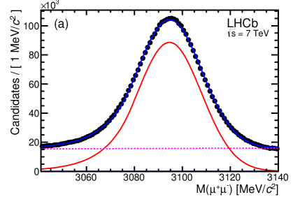
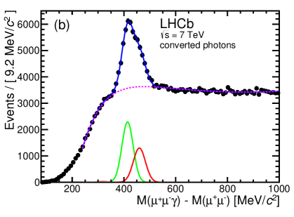
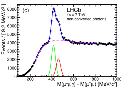
Figure 1: (a) Invariant mass of the $\mu^{+}\mu^{-}$ pair for selected ${J\mskip-3.0mu/\mskip-2.0mu\psi\mskip 2.0mu}$ candidates. The solid red curve corresponds to the signal and the background is shown as a dashed purple curve. (b) and (c) show the $\Delta M\,{=}\,M\left(\mu^{+}\mu^{-}\,\gamma\right)\,{-}\,M\left(\mu^{+}\mu^{-}\right)$ distributions of selected $\chi_{c}$ candidates with (b) converted and (c) non-converted photons. The upper solid blue curve corresponds to the overall fit function described in Ref. [3]. The lower solid curves correspond to the fitted $\chi_{c0}$, $\chi_{c1}$ and $\chi_{c2}$ contributions from left to right, respectively (the $\chi_{c0}$ peak is barely visible). The background distribution is shown as a dashed purple curve.

3 Determination of the cross-section ratio

The main contributions to the production of prompt ${J\mskip-3.0mu/\mskip-2.0mu\psi\mskip 2.0mu}$ arise from direct production and from the feed-down processes $\chi_{c}\rightarrow{J\mskip-3.0mu/\mskip-2.0mu\psi\mskip 2.0mu}\gamma$ and $\psi{(2S)}\rightarrow{J\mskip-3.0mu/\mskip-2.0mu\psi\mskip 2.0mu}X$ where $X$ refers to any final state. The cross-section ratio for the production of prompt ${J\mskip-3.0mu/\mskip-2.0mu\psi\mskip 2.0mu}$ from $\chi_{c}\rightarrow{J\mskip-3.0mu/\mskip-2.0mu\psi\mskip 2.0mu}\gamma$ decays compared to all prompt ${J\mskip-3.0mu/\mskip-2.0mu\psi\mskip 2.0mu}$ can be expressed in terms of the three $\chi_{cJ}$ $(J=0,1,2)$ signal yields, $N_{\chi_{cJ}}$, and the prompt ${J\mskip-3.0mu/\mskip-2.0mu\psi\mskip 2.0mu}$ yield, $N_{{J\mskip-3.0mu/\mskip-2.0mu\psi\mskip 2.0mu}}$, as

$$\dfrac{\sigma(\chi_{c}\rightarrow{J\mskip-3.0mu/\mskip-2.0mu\psi\mskip 2.0mu}\gamma)}{\sigma({J\mskip-3.0mu/\mskip-2.0mu\psi\mskip 2.0mu})} \,\approx\,\dfrac{\sigma(\chi_{c}\rightarrow{J\mskip-3.0mu/\mskip-2.0mu\psi\mskip 2.0mu}\gamma)}{\sigma^{\mathrm{dir}}({J\mskip-3.0mu/\mskip-2.0mu\psi\mskip 2.0mu})+\sigma(\psi{(2S)}\rightarrow{J\mskip-3.0mu/\mskip-2.0mu\psi\mskip 2.0mu}X)+\sigma(\chi_{c}\rightarrow{J\mskip-3.0mu/\mskip-2.0mu\psi\mskip 2.0mu}\gamma)}$$

$$\,\,{=}\,\,\dfrac{\displaystyle{\sum_{J=0}^{J=2}}\;\dfrac{N_{\chi_{cJ}}}{\epsilon^{\chi_{cJ}}_{\gamma}\epsilon^{\chi_{cJ}}_{\mathrm{sel}}}\cdot\dfrac{\epsilon^{\mathrm{dir}}_{{J\mskip-3.0mu/\mskip-2.0mu\psi\mskip 2.0mu}}}{\epsilon^{\chi_{cJ}}_{{J\mskip-3.0mu/\mskip-2.0mu\psi\mskip 2.0mu}}}}{N_{{J\mskip-3.0mu/\mskip-2.0mu\psi\mskip 2.0mu}}R_{2S}+\displaystyle{\sum_{J=0}^{J=2}}\;\dfrac{N_{\chi_{cJ}}}{\epsilon^{\chi_{cJ}}_{\gamma}\epsilon^{\chi_{cJ}}_{\mathrm{sel}}}\left[\dfrac{\epsilon^{\mathrm{dir}}_{{J\mskip-3.0mu/\mskip-2.0mu\psi\mskip 2.0mu}}}{\epsilon^{\chi_{cJ}}_{{J\mskip-3.0mu/\mskip-2.0mu\psi\mskip 2.0mu}}}-R_{2S}\right]}$$ (1)

with

$$R_{2S} \,\,{=}\,\,\dfrac{1+f_{2S}}{1+f_{2S}\dfrac{\epsilon_{{J\mskip-3.0mu/\mskip-2.0mu\psi\mskip 2.0mu}}^{2S}}{\epsilon_{{J\mskip-3.0mu/\mskip-2.0mu\psi\mskip 2.0mu}}^{\mathrm{dir}}}}$$ (2)

and

$$f_{2S} \,\,{=}\,\,\dfrac{\sigma(\psi{(2S)}\rightarrow{J\mskip-3.0mu/\mskip-2.0mu\psi\mskip 2.0mu}X)}{\sigma^{\mathrm{dir}}({J\mskip-3.0mu/\mskip-2.0mu\psi\mskip 2.0mu})}.$$ (3)

The total prompt $\chi_{c}\rightarrow{J\mskip-3.0mu/\mskip-2.0mu\psi\mskip 2.0mu}\gamma$ cross-section is $\sigma(\chi_{c}\rightarrow{J\mskip-3.0mu/\mskip-2.0mu\psi\mskip 2.0mu}\gamma)=\sum_{J=0}^{J=2}\;\sigma_{\chi_{cJ}}\cdot{\cal B}(\chi_{cJ}\rightarrow{J\mskip-3.0mu/\mskip-2.0mu\psi\mskip 2.0mu}\gamma)$ where $\sigma_{\chi_{cJ}}$ is the production cross-section for each $\chi_{cJ}$ state and $\cal B$($\chi_{cJ}\rightarrow{J\mskip-3.0mu/\mskip-2.0mu\psi\mskip 2.0mu}\gamma$) is the corresponding branching fraction. The cross-section ratio $f_{2S}$ is used to link the prompt $\psi{(2S)}$ contribution to the direct ${J\mskip-3.0mu/\mskip-2.0mu\psi\mskip 2.0mu}$ contribution and $R_{2S}$ takes into account their efficiencies. The combination of the trigger, reconstruction and selection efficiencies for direct ${J\mskip-3.0mu/\mskip-2.0mu\psi\mskip 2.0mu}$, for ${J\mskip-3.0mu/\mskip-2.0mu\psi\mskip 2.0mu}$ from $\psi{(2S)}$ decay, and for ${J\mskip-3.0mu/\mskip-2.0mu\psi\mskip 2.0mu}$ from $\chi_{c}\rightarrow{J\mskip-3.0mu/\mskip-2.0mu\psi\mskip 2.0mu}\gamma$ decay are $\epsilon^{\mathrm{dir}}_{{J\mskip-3.0mu/\mskip-2.0mu\psi\mskip 2.0mu}}$, $\epsilon^{2S}_{{J\mskip-3.0mu/\mskip-2.0mu\psi\mskip 2.0mu}}$, and $\epsilon^{\chi_{cJ}}_{{J\mskip-3.0mu/\mskip-2.0mu\psi\mskip 2.0mu}}$ respectively. The efficiency to reconstruct and select a photon from a $\chi_{c}\rightarrow{J\mskip-3.0mu/\mskip-2.0mu\psi\mskip 2.0mu}\gamma$ decay, once the ${J\mskip-3.0mu/\mskip-2.0mu\psi\mskip 2.0mu}$ is already selected, is $\epsilon^{\chi_{cJ}}_{\gamma}$ and the efficiency for the subsequent selection of the $\chi_{cJ}$ is $\epsilon^{\chi_{cJ}}_{\mathrm{sel}}$.

The efficiency terms in Eq. (1) are determined using simulated events and are partly validated with control channels in the data. The results for the efficiency ratios $\epsilon^{2S}_{{J\mskip-3.0mu/\mskip-2.0mu\psi\mskip 2.0mu}}/\epsilon^{\mathrm{dir}}_{{J\mskip-3.0mu/\mskip-2.0mu\psi\mskip 2.0mu}}$, $\epsilon^{\mathrm{dir}}_{{J\mskip-3.0mu/\mskip-2.0mu\psi\mskip 2.0mu}}/\epsilon^{\chi_{cJ}}_{{J\mskip-3.0mu/\mskip-2.0mu\psi\mskip 2.0mu}}$ and the product $\epsilon^{\chi_{cJ}}_{\gamma}\epsilon^{\chi_{cJ}}_{\mathrm{sel}}$ are discussed in Sect. 4.

The prompt $N_{{J\mskip-3.0mu/\mskip-2.0mu\psi\mskip 2.0mu}}$ and $N_{\chi_{cJ}}$ yields are determined in bins of $p_{\mathrm{T}}^{{J\mskip-3.0mu/\mskip-2.0mu\psi\mskip 2.0mu}}$ in the range $2\,{<}\,p_{\mathrm{T}}^{{J\mskip-3.0mu/\mskip-2.0mu\psi\mskip 2.0mu}}\,{<}\,15~{}{\mathrm{\,Ge\kern-1.00006ptV\!/}c}$ using the methods described in Refs. [2] and [3] respectively. In Ref. [2] a smaller data sample is used to determine the non-prompt ${J\mskip-3.0mu/\mskip-2.0mu\psi\mskip 2.0mu}$ fractions in bins of $p_{\mathrm{T}}^{{J\mskip-3.0mu/\mskip-2.0mu\psi\mskip 2.0mu}}$ and rapidity. These results are applied to the present ${J\mskip-3.0mu/\mskip-2.0mu\psi\mskip 2.0mu}$ sample without repeating the full analysis.

4 Efficiencies

The efficiencies to reconstruct and select ${J\mskip-3.0mu/\mskip-2.0mu\psi\mskip 2.0mu}$ and $\chi_{c}$  candidates are taken from simulation. The efficiency ratio $\epsilon^{2S}_{{J\mskip-3.0mu/\mskip-2.0mu\psi\mskip 2.0mu}}/\epsilon^{\mathrm{dir}}_{{J\mskip-3.0mu/\mskip-2.0mu\psi\mskip 2.0mu}}$ is consistent with unity for all $p_{\mathrm{T}}^{{J\mskip-3.0mu/\mskip-2.0mu\psi\mskip 2.0mu}}$ bins; hence, $R_{2S}$ is set equal to 1 in Eq. (2). The ratio of efficiencies $\epsilon^{\mathrm{dir}}_{{J\mskip-3.0mu/\mskip-2.0mu\psi\mskip 2.0mu}}/\epsilon^{\chi_{cJ}}_{{J\mskip-3.0mu/\mskip-2.0mu\psi\mskip 2.0mu}}$ and the product of efficiencies $\epsilon^{\chi_{cJ}}_{\gamma}\epsilon^{\chi_{cJ}}_{\mathrm{sel}}$ for the $\chi_{c1}$ and $\chi_{c2}$ states are shown in Fig. 2. In general these efficiencies are the same for the two states, except at low $p_{\mathrm{T}}^{{J\mskip-3.0mu/\mskip-2.0mu\psi\mskip 2.0mu}}$ where the reconstruction and detection efficiencies for $\chi_{c2}$ are significantly larger than for $\chi_{c1}$. This difference arises from the effect of the requirement $p_{\mathrm{T}}^{\gamma}\,{>}\,\mbox{${650}\>{{\mathrm{\,Me\kern-1.00006ptV\!/}c}}$}$ which results in more photons surviving from $\chi_{c2}$ decays than from $\chi_{c1}$ decays.

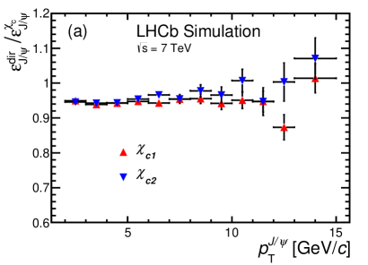
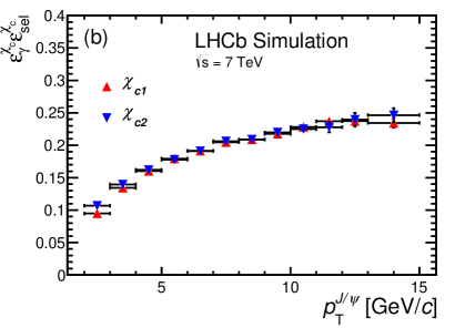
Figure 2: (a) Ratio of the reconstruction and selection efficiency for direct ${J\mskip-3.0mu/\mskip-2.0mu\psi\mskip 2.0mu}$ compared to ${J\mskip-3.0mu/\mskip-2.0mu\psi\mskip 2.0mu}$ from $\chi_{c}$ decays, $\epsilon^{\mathrm{dir}}_{{J\mskip-3.0mu/\mskip-2.0mu\psi\mskip 2.0mu}}/\epsilon^{\chi_{c}}_{{J\mskip-3.0mu/\mskip-2.0mu\psi\mskip 2.0mu}}$, and (b) the photon reconstruction and selection efficiency multiplied by the $\chi_{c}$ selection efficiency, $\epsilon^{\chi_{cJ}}_{\gamma}\epsilon^{\chi_{cJ}}_{\mathrm{sel}}$, obtained from simulation. The efficiencies are presented separately for the $\chi_{c1}$ (red triangles) and $\chi_{c2}$ (inverted blue triangles) states, and as a function of $p_{\mathrm{T}}^{{J\mskip-3.0mu/\mskip-2.0mu\psi\mskip 2.0mu}}$.

The photon detection efficiency obtained using simulation is validated using candidate $B^{+}\rightarrow{J\mskip-3.0mu/\mskip-2.0mu\psi\mskip 2.0mu}K^{+}$ and $B^{+}\rightarrow\chi_{c}K^{+}$ (including charge conjugate) decays selected from the same data set as the prompt ${J\mskip-3.0mu/\mskip-2.0mu\psi\mskip 2.0mu}$ and $\chi_{c}$ candidates. The efficiency to reconstruct and select a photon from a $\chi_{c}$ in $B^{+}\rightarrow\chi_{c}K^{+}$ decays, $\epsilon_{\gamma}$, is evaluated using

$$\epsilon_{\gamma}\,{=}\,\frac{N_{B^{+}\rightarrow\chi_{c}K^{+}}}{N_{B^{+}\rightarrow{J\mskip-3.0mu/\mskip-2.0mu\psi\mskip 2.0mu}K^{+}}}\times\frac{{\cal B}(B^{+}\rightarrow{J\mskip-3.0mu/\mskip-2.0mu\psi\mskip 2.0mu}K^{+})}{{\cal B}(B^{+}\rightarrow\chi_{c}K^{+})\cdot{\cal B}(\chi_{c}\rightarrow{J\mskip-3.0mu/\mskip-2.0mu\psi\mskip 2.0mu}\gamma)}\times R_{\epsilon}$$ (4)

where $N_{B^{+}\rightarrow\chi_{c}K^{+}}$ and $N_{B^{+}\rightarrow{J\mskip-3.0mu/\mskip-2.0mu\psi\mskip 2.0mu}K^{+}}$ are the measured yields of $B^{+}\rightarrow\chi_{c}K^{+}$ and $B^{+}\rightarrow{J\mskip-3.0mu/\mskip-2.0mu\psi\mskip 2.0mu}K^{+}$ and ${\cal B}$ are the known branching fractions. The factor $R_{\epsilon}=1.04\pm 0.02$ is obtained from simulation and takes into account any differences in the acceptance, trigger, selection and reconstruction efficiencies of the $K$, ${J\mskip-3.0mu/\mskip-2.0mu\psi\mskip 2.0mu}$, $\chi_{c}$ (except the photon detection efficiency) and $B^{+}$ in $B^{+}\rightarrow{J\mskip-3.0mu/\mskip-2.0mu\psi\mskip 2.0mu}K^{+}$ and $B^{+}\rightarrow\chi_{c}K^{+}$ decays. All branching fractions are taken from Ref. [12]. The $B^{+}\rightarrow{J\mskip-3.0mu/\mskip-2.0mu\psi\mskip 2.0mu}K^{+}$ branching fraction is ${\cal B}(B^{+}\rightarrow{J\mskip-3.0mu/\mskip-2.0mu\psi\mskip 2.0mu}K^{+})=(1.013\pm 0.034)\times 10^{-3}$. The dominant process for $B^{+}\rightarrow\chi_{c}K^{+}\rightarrow{J\mskip-3.0mu/\mskip-2.0mu\psi\mskip 2.0mu}\gamma K^{+}$ decays is via the $\chi_{c1}$ state, with branching fractions ${\cal B}(B^{+}\rightarrow\chi_{c1}K^{+})=(4.6\pm 0.4)\times 10^{-4}$ and ${\cal B}(\chi_{c1}\rightarrow{J\mskip-3.0mu/\mskip-2.0mu\psi\mskip 2.0mu}\gamma)=(34.4\pm 1.5)\times 10^{-2}$; the contributions from the $\chi_{c0}$ and $\chi_{c2}$ modes are neglected.

The $B^{+}\rightarrow\chi_{c}K^{+}$ and $B^{+}\rightarrow{J\mskip-3.0mu/\mskip-2.0mu\psi\mskip 2.0mu}K^{+}$ candidates are selected keeping as many of the selection criteria in common as possible with the main analysis. The ${J\mskip-3.0mu/\mskip-2.0mu\psi\mskip 2.0mu}$ and $\chi_{c}$ selection criteria are the same as for the prompt analysis, apart from the pseudo-decay time requirement. The bachelor kaon is required to have a well measured track ($\chi^{2}/\mathrm{ndf}<5$), a minimum impact parameter $\chi^{2}$ with respect to all primary vertices of greater than $9$ and a momentum greater than $5\,{\mathrm{\,Ge\kern-1.00006ptV\!/}c}$. The bachelor is identified as a kaon by the RICH detectors by requiring the difference in log-likelihoods between the kaon and pion hypotheses to be larger than $5$. The $B$ candidate is formed from the $\chi_{c}$ or ${J\mskip-3.0mu/\mskip-2.0mu\psi\mskip 2.0mu}$ candidate and the bachelor kaon. The $B$ vertex is required to be well measured ($\chi^{2}/\mathrm{ndf}<9$) and separated from the primary vertex (flight distance $\chi^{2}>50$). The $B$ momentum vector is required to point towards the primary vertex ($\cos\theta>0.9999$, where $\theta$ is the angle between the $B$ momentum and the direction between the primary and $B$ vertices) and have an impact parameter $\chi^{2}$ smaller than $9$. The combinatorial background under the $\chi_{c}$ peak for the $B^{+}\rightarrow\chi_{c}K^{+}$ candidates is reduced by requiring the mass difference $\Delta M_{\chi_{c}}=M(\mu^{+}\mu^{-}\gamma)-M(\mu^{+}\mu^{-})<600{\mathrm{\,Me\kern-1.00006ptV\!/}c^{2}}$. A small number of $B^{+}\rightarrow\chi_{c}K^{+}$ candidates which form a good $B^{+}\rightarrow{J\mskip-3.0mu/\mskip-2.0mu\psi\mskip 2.0mu}K^{+}$ candidate are removed by requiring $|M(\mu^{+}\mu^{-}\gamma K)-M(\mu^{+}\mu^{-}K)|>200{\mathrm{\,Me\kern-1.00006ptV\!/}c^{2}}$.

The $\Delta M_{B^{+}}=M(\mu^{+}\mu^{-}\gamma K)-M(\mu^{+}\mu^{-}\gamma)$ mass distribution for the $B^{+}\rightarrow\chi_{c}K^{+}$ candidates is shown in Fig. 3(a); $\Delta M_{B^{+}}$ is computed to improve the resolution and hence the signal-to-background ratio. The $B^{+}\rightarrow\chi_{c}K^{+}$ yield, $142\pm 15$ candidates, is determined from a fit that uses a Gaussian function to describe the signal peak and a threshold function,

$$f(x)\,{=}\,x^{a}\!\left(1-e^{\frac{m_{0}}{c}\left(1-x\right)}\right)+b\left(x-1\right),$$ (5)

where $x\,{=}\,\Delta M_{B^{+}}\,{/}\,m_{0}$ and $m_{0}$, $a$, $b$ and $c$ are free parameters, to model the background. The reconstructed $B^{+}$ mass distribution for the $B^{+}\rightarrow{J\mskip-3.0mu/\mskip-2.0mu\psi\mskip 2.0mu}K^{+}$ candidates is shown in Fig. 3(b). The $B^{+}\rightarrow{J\mskip-3.0mu/\mskip-2.0mu\psi\mskip 2.0mu}K^{+}$ yield, $8440\pm 96$ candidates, is determined from a fit that uses a Crystal Ball function [13] to describe the signal peak and an exponential to model the background.

The photon efficiency from the observation of $B^{+}\rightarrow\chi_{c}K^{+}$ and $B^{+}\rightarrow{J\mskip-3.0mu/\mskip-2.0mu\psi\mskip 2.0mu}K^{+}$ decays is measured to be $\epsilon_{\gamma}=(11.3\pm 1.2\pm 1.2)\%$ where the first error is statistical and is dominated by the observed yield of $B^{+}\rightarrow\chi_{c}K^{+}$ candidates, and the second error is systematic and is given by the uncertainty on the branching fraction $\cal B$($B^{+}\rightarrow\chi_{c1}K^{+}$). The photon efficiency measured in data can be compared to the photon efficiency, $(11.7\pm 0.3)\%$, obtained using the same procedure on simulated events. The measurements are in good agreement and the uncertainty on the difference between data and simulation is propagated as a $\pm 14\%$ relative systematic uncertainty on the photon efficiency in the measurement of $\sigma(\chi_{c}\rightarrow{J\mskip-3.0mu/\mskip-2.0mu\psi\mskip 2.0mu}\gamma)\,/\,\sigma({J\mskip-3.0mu/\mskip-2.0mu\psi\mskip 2.0mu})$.

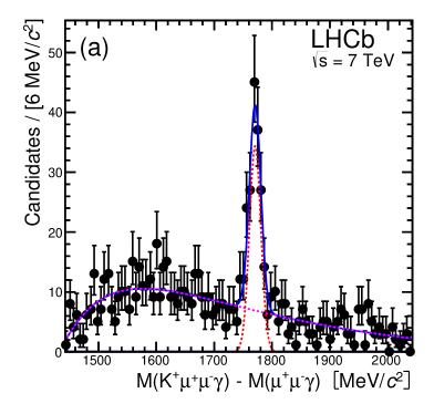
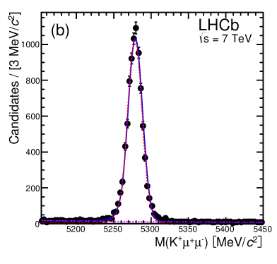
Figure 3: (a) Reconstructed $\Delta M_{B^{+}}=M(\mu^{+}\mu^{-}\gamma K)-M(\mu^{+}\mu^{-}\gamma)$ mass distribution for $B^{+}\rightarrow\chi_{c}K^{+}$ candidates and (b) the reconstructed $B^{+}$ mass distribution for $B^{+}\rightarrow{J\mskip-3.0mu/\mskip-2.0mu\psi\mskip 2.0mu}K^{+}$ candidates. The LHCb data are shown as solid black points, the full fit functions with a solid blue (upper) curve, the contribution from signal candidates with a dashed red (lower curve) and the background with a dashed purple curve.

5 Polarisation

The simulation used to calculate the efficiencies and, hence, extract the result of Eq. (1) assumes that the ${J\mskip-3.0mu/\mskip-2.0mu\psi\mskip 2.0mu}$ and $\chi_{c}$ are unpolarised. The effect of polarised states is studied by reweighting the simulated events according to different polarisation scenarios; the results are shown in Table 1. It is also noted that, since the $\psi{(2S)}$ decays predominantly to ${J\mskip-3.0mu/\mskip-2.0mu\psi\mskip 2.0mu}\pi\pi$, with the $\pi\pi$ in an $S$ wave state [14], and the $\psi{(2S)}$ polarisation should not differ significantly from the polarisation of directly produced ${J\mskip-3.0mu/\mskip-2.0mu\psi\mskip 2.0mu}$ mesons, the effect of the polarisation can be considered independent of the $\psi{(2S)}\rightarrow{J\mskip-3.0mu/\mskip-2.0mu\psi\mskip 2.0mu}X$ contribution [15].

The ${J\mskip-3.0mu/\mskip-2.0mu\psi\mskip 2.0mu}$ and $\chi_{c}\rightarrow{J\mskip-3.0mu/\mskip-2.0mu\psi\mskip 2.0mu}\gamma$ angular distributions are calculated in the helicity frame assuming azimuthal symmetry. This choice of reference frame provides an estimate of the effect of polarisation on the results, pending the direct measurements of the ${J\mskip-3.0mu/\mskip-2.0mu\psi\mskip 2.0mu}$ and $\chi_{c}$ polarisations. The ${J\mskip-3.0mu/\mskip-2.0mu\psi\mskip 2.0mu}$ system is described by the angle $\theta_{{J\mskip-3.0mu/\mskip-2.0mu\psi\mskip 2.0mu}}$, which is the angle between the directions of the $\mu^{+}$ in the ${J\mskip-3.0mu/\mskip-2.0mu\psi\mskip 2.0mu}$ rest frame and the ${J\mskip-3.0mu/\mskip-2.0mu\psi\mskip 2.0mu}$ in the laboratory frame. The $\theta_{{J\mskip-3.0mu/\mskip-2.0mu\psi\mskip 2.0mu}}$ distribution depends on the parameter $\lambda_{{J\mskip-3.0mu/\mskip-2.0mu\psi\mskip 2.0mu}}$ which describes the ${J\mskip-3.0mu/\mskip-2.0mu\psi\mskip 2.0mu}$ polarisation; $\lambda_{{J\mskip-3.0mu/\mskip-2.0mu\psi\mskip 2.0mu}}=+1,-1,0$ corresponds to pure transverse, pure longitudinal and no polarisation respectively. The $\chi_{c}\rightarrow{J\mskip-3.0mu/\mskip-2.0mu\psi\mskip 2.0mu}\gamma$ system is described by three angles: $\theta^{\prime}_{{J\mskip-3.0mu/\mskip-2.0mu\psi\mskip 2.0mu}}$, $\theta_{\chi_{c}}$ and $\phi$, where $\theta^{\prime}_{{J\mskip-3.0mu/\mskip-2.0mu\psi\mskip 2.0mu}}$ is the angle between the directions of the $\mu^{+}$ in the ${J\mskip-3.0mu/\mskip-2.0mu\psi\mskip 2.0mu}$ rest frame and the ${J\mskip-3.0mu/\mskip-2.0mu\psi\mskip 2.0mu}$ in the $\chi_{c}$ rest frame, $\theta_{\chi_{c}}$ is the angle between the directions of the ${J\mskip-3.0mu/\mskip-2.0mu\psi\mskip 2.0mu}$ in the $\chi_{c}$ rest frame and the $\chi_{c}$ in the laboratory frame, and $\phi$ is the angle between the ${J\mskip-3.0mu/\mskip-2.0mu\psi\mskip 2.0mu}$ decay plane in the $\chi_{c}$ rest frame and the plane formed by the $\chi_{c}$ direction in the laboratory frame and the direction of the ${J\mskip-3.0mu/\mskip-2.0mu\psi\mskip 2.0mu}$ in the $\chi_{c}$ rest frame. The general expressions for the angular distributions are independent of the choice of polarisation axis (here chosen as the direction of the $\chi_{c}$ in the laboratory frame) and are detailed in Ref. [4]. The angular distributions of the $\chi_{c}$ states depend on $m_{\chi_{cJ}}$ which is the azimuthal angular momentum quantum number of the $\chi_{cJ}$ state.

For each simulated event in the unpolarised sample, a weight is calculated from the distributions of $\theta^{\prime}_{{J\mskip-3.0mu/\mskip-2.0mu\psi\mskip 2.0mu}}$, $\theta_{\chi_{c}}$ and $\phi$ in the various polarisation hypotheses compared to the unpolarised distributions. The weights shown in Table 1 are then the average of these per-event weights in the simulated sample. For a given ($|m_{\chi_{c1}}|$, $|m_{\chi_{c2}}|$, $\lambda_{{J\mskip-3.0mu/\mskip-2.0mu\psi\mskip 2.0mu}}$) polarisation combination, the central value of the determined cross-section ratio in each $p_{\mathrm{T}}^{{J\mskip-3.0mu/\mskip-2.0mu\psi\mskip 2.0mu}}$ bin should be multiplied by the number in the table. The maximum effect from the possible polarisation of the ${J\mskip-3.0mu/\mskip-2.0mu\psi\mskip 2.0mu}$, $\chi_{c1}$ and $\chi_{c2}$ mesons is given separately from the systematic uncertainties in Table 3 and Fig. 4.

Table 1: Polarisation weights in $p_{\mathrm{T}}^{{J\mskip-3.0mu/\mskip-2.0mu\psi\mskip 2.0mu}}$ bins for different combinations of the ${J\mskip-3.0mu/\mskip-2.0mu\psi\mskip 2.0mu}$, $\chi_{c1}$ and $\chi_{c2}$ polarisations. $\lambda_{{J\mskip-3.0mu/\mskip-2.0mu\psi\mskip 2.0mu}}$ is the ${J\mskip-3.0mu/\mskip-2.0mu\psi\mskip 2.0mu}$ polarisation parameter; $\lambda_{{J\mskip-3.0mu/\mskip-2.0mu\psi\mskip 2.0mu}}=+1,-1,0$ corresponds to fully transverse, fully longitudinal and no polarisation respectively. $m_{\chi_{cJ}}$ is the azimuthal angular momentum quantum number corresponding to total angular momentum $J$; Unpol means the $\chi_{c}$ is unpolarised.

($|m_{\chi_{c1}}|,|m_{\chi_{c2}}|,\lambda_{{J\mskip-3.0mu/\mskip-2.0mu\psi\mskip 2.0mu}}$)	$p_{\mathrm{T}}^{{J\mskip-3.0mu/\mskip-2.0mu\psi\mskip 2.0mu}}$ (${\mathrm{\,Ge\kern-0.50003ptV\!/}c}$)
	2-3	3-4	4-5	5-6	6-7	7-8	8-9	9-10	10-11	11-12	12-13	13-15
(Unpol,Unpol,-1)	1.16	1.15	1.15	1.15	1.15	1.14	1.14	1.13	1.12	1.12	1.10	1.10
(Unpol,Unpol,1)	0.92	0.92	0.92	0.92	0.92	0.92	0.93	0.93	0.93	0.94	0.95	0.94
(Unpol,0,-1)	1.16	1.14	1.13	1.11	1.10	1.09	1.09	1.08	1.07	1.06	1.06	1.07
(Unpol,0,0)	1.00	0.99	0.98	0.97	0.96	0.95	0.95	0.96	0.95	0.95	0.96	0.97
(Unpol,0,1)	0.91	0.91	0.90	0.89	0.88	0.87	0.88	0.89	0.89	0.88	0.91	0.92
(Unpol,1,-1)	1.15	1.14	1.14	1.13	1.13	1.12	1.11	1.11	1.10	1.09	1.08	1.09
(Unpol,1,0)	0.99	0.99	0.99	0.98	0.98	0.98	0.98	0.98	0.98	0.98	0.98	0.98
(Unpol,1,1)	0.90	0.91	0.91	0.90	0.90	0.90	0.91	0.91	0.91	0.91	0.93	0.93
(Unpol,2,-1)	1.18	1.17	1.18	1.20	1.21	1.21	1.20	1.19	1.19	1.19	1.16	1.15
(Unpol,2,0)	1.01	1.02	1.03	1.04	1.05	1.06	1.06	1.05	1.06	1.07	1.05	1.04
(Unpol,2,1)	0.93	0.94	0.94	0.96	0.97	0.98	0.98	0.98	0.99	1.00	1.00	0.99
(0,Unpol,-1)	1.16	1.15	1.18	1.21	1.22	1.23	1.25	1.25	1.26	1.22	1.23	1.25
(0,Unpol,0)	0.99	1.00	1.02	1.05	1.07	1.08	1.10	1.11	1.12	1.10	1.12	1.14
(0,Unpol,1)	0.91	0.93	0.94	0.97	0.98	1.00	1.02	1.04	1.05	1.03	1.06	1.08
(1,Unpol,-1)	1.17	1.15	1.14	1.13	1.12	1.11	1.09	1.08	1.07	1.08	1.05	1.05
(1,Unpol,0)	1.00	1.00	0.99	0.98	0.97	0.97	0.96	0.95	0.95	0.96	0.95	0.95
(1,Unpol,1)	0.92	0.92	0.91	0.90	0.89	0.89	0.89	0.89	0.89	0.90	0.90	0.89
(0,0,-1)	1.15	1.14	1.15	1.17	1.18	1.18	1.20	1.21	1.20	1.17	1.19	1.22
(0,0,0)	0.99	0.99	1.00	1.02	1.02	1.03	1.05	1.07	1.07	1.04	1.08	1.11
(0,0,1)	0.91	0.91	0.92	0.93	0.94	0.95	0.98	1.00	1.00	0.98	1.02	1.05
(0,1,-1)	1.14	1.14	1.16	1.19	1.20	1.21	1.22	1.23	1.23	1.20	1.21	1.24
(0,1,0)	0.98	0.99	1.01	1.03	1.05	1.06	1.08	1.09	1.10	1.07	1.10	1.12
(0,1,1)	0.90	0.92	0.93	0.95	0.96	0.98	1.00	1.02	1.03	1.01	1.04	1.07
(0,2,-1)	1.17	1.17	1.21	1.25	1.29	1.30	1.31	1.31	1.32	1.30	1.28	1.30
(0,2,0)	1.01	1.02	1.05	1.09	1.12	1.14	1.16	1.17	1.19	1.17	1.17	1.18
(0,2,1)	0.92	0.94	0.96	1.01	1.03	1.06	1.08	1.09	1.11	1.10	1.11	1.12
(1,0,-1)	1.16	1.13	1.12	1.09	1.07	1.05	1.04	1.04	1.02	1.02	1.01	1.01
(1,0,0)	1.00	0.99	0.97	0.94	0.93	0.92	0.91	0.91	0.90	0.91	0.91	0.92
(1,0,1)	0.92	0.91	0.89	0.87	0.85	0.84	0.85	0.85	0.84	0.85	0.86	0.86
(1,1,-1)	1.15	1.14	1.13	1.11	1.10	1.08	1.07	1.06	1.05	1.05	1.03	1.03
(1,1,0)	0.99	0.99	0.98	0.96	0.95	0.94	0.94	0.94	0.93	0.94	0.94	0.93
(1,1,1)	0.91	0.91	0.90	0.88	0.87	0.87	0.87	0.87	0.87	0.88	0.88	0.88
(1,2,-1)	1.18	1.17	1.17	1.17	1.18	1.18	1.16	1.14	1.14	1.15	1.11	1.09
(1,2,0)	1.02	1.01	1.01	1.02	1.03	1.03	1.02	1.01	1.02	1.03	1.01	0.99
(1,2,1)	0.93	0.94	0.93	0.94	0.94	0.95	0.94	0.94	0.95	0.97	0.95	0.93

6 Systematic uncertainties

Table 2: Summary of the systematic uncertainties on $\sigma(\chi_{c}\rightarrow{J\mskip-3.0mu/\mskip-2.0mu\psi\mskip 2.0mu}\gamma)\,/\,\sigma({J\mskip-3.0mu/\mskip-2.0mu\psi\mskip 2.0mu})$ in each $p_{\mathrm{T}}^{{J\mskip-3.0mu/\mskip-2.0mu\psi\mskip 2.0mu}}$ bin.

$p_{\mathrm{T}}^{{J\mskip-3.0mu/\mskip-2.0mu\psi\mskip 2.0mu}}$(${\mathrm{\,Ge\kern-0.80005ptV\!/}c}$)	$2-3$	$3-4$	$4-5$	$5-6$	$6-7$	$7-8$
Size of simulation sample	${}^{+0.0006}_{-0.0005}$	${}^{+0.0006}_{-0.0005}$	${}^{+0.0007}_{-0.0006}$	${}^{+0.0009}_{-0.0009}$	${}^{+0.001}_{-0.001}$	${}^{+0.002}_{-0.002}$
Photon efficiency	${}^{+0.011}_{-0.010}$	${}^{+0.013}_{-0.011}$	${}^{+0.013}_{-0.012}$	${}^{+0.016}_{-0.013}$	${}^{+0.016}_{-0.013}$	${}^{+0.017}_{-0.015}$
Non-prompt ${J\mskip-3.0mu/\mskip-2.0mu\psi\mskip 2.0mu}$ fraction	${}^{+0.002}_{-0.005}$	${}^{+0.003}_{-0.005}$	${}^{+0.003}_{-0.006}$	${}^{+0.004}_{-0.008}$	${}^{+0.005}_{-0.010}$	${}^{+0.006}_{-0.011}$
Fit model	${}^{+0.003}_{-0.003}$	${}^{+0.003}_{-0.003}$	${}^{+0.002}_{-0.004}$	${}^{+0.003}_{-0.005}$	${}^{+0.002}_{-0.005}$	${}^{+0.003}_{-0.006}$
Simulation calibration	${}^{+0.010}_{-0.000}$	${}^{+0.010}_{-0.000}$	${}^{+0.012}_{-0.000}$	${}^{+0.012}_{-0.000}$	${}^{+0.015}_{-0.000}$	${}^{+0.014}_{-0.000}$
$p_{\mathrm{T}}^{{J\mskip-3.0mu/\mskip-2.0mu\psi\mskip 2.0mu}}$(${\mathrm{\,Ge\kern-0.80005ptV\!/}c}$)	$8-9$	$9-10$	$10-11$	$11-12$	$12-13$	$13-15$
Size of simulation sample	${}^{+0.002}_{-0.002}$	${}^{+0.003}_{-0.003}$	${}^{+0.004}_{-0.004}$	${}^{+0.006}_{-0.006}$	${}^{+0.008}_{-0.008}$	${}^{+0.008}_{-0.008}$
Photon efficiency	${}^{+0.018}_{-0.016}$	${}^{+0.020}_{-0.016}$	${}^{+0.019}_{-0.016}$	${}^{+0.019}_{-0.018}$	${}^{+0.021}_{-0.020}$	${}^{+0.023}_{-0.019}$
Non-prompt ${J\mskip-3.0mu/\mskip-2.0mu\psi\mskip 2.0mu}$ fraction	${}^{+0.009}_{-0.011}$	${}^{+0.012}_{-0.013}$	${}^{+0.011}_{-0.017}$	${}^{+0.019}_{-0.019}$	${}^{+0.022}_{-0.018}$	${}^{+0.018}_{-0.010}$
Fit model	${}^{+0.002}_{-0.005}$	${}^{+0.002}_{-0.003}$	${}^{+0.006}_{-0.002}$	${}^{+0.001}_{-0.006}$	${}^{+0.003}_{-0.008}$	${}^{+0.002}_{-0.004}$
Simulation calibration	${}^{+0.015}_{-0.000}$	${}^{+0.017}_{-0.000}$	${}^{+0.018}_{-0.000}$	${}^{+0.018}_{-0.000}$	${}^{+0.017}_{-0.000}$	${}^{+0.022}_{-0.000}$

The systematic uncertainties detailed below are measured by repeatedly sampling from the distribution of the parameter under consideration. For each sampled value, the cross-section ratio is calculated and the $68.3\%$ probability interval is determined from the resulting distribution.

The statistical errors from the finite number of simulated events used for the calculation of the efficiencies are included as a systematic uncertainty in the final results. The uncertainty is determined by sampling the efficiencies used in Eq. 1 according to their errors. The relative systematic uncertainty due to the limited size of the simulation sample is found to be in the range ${(0.3}\,{-}\,{3.2)\%}$ and is given for each $p_{\mathrm{T}}^{{J\mskip-3.0mu/\mskip-2.0mu\psi\mskip 2.0mu}}$ bin in Table 2.

The efficiency extracted from the simulation sample for reconstructing and selecting a photon in $\chi_{c}\rightarrow{J\mskip-3.0mu/\mskip-2.0mu\psi\mskip 2.0mu}\gamma$ decays has been validated using $B^{+}\rightarrow\chi_{c}K^{+}$ and $B^{+}\rightarrow{J\mskip-3.0mu/\mskip-2.0mu\psi\mskip 2.0mu}K^{+}$ decays observed in the data, as described in Sect. 4. The relative uncertainty between the photon efficiencies measured in the data and simulation, $\pm 14\%$, arises from the finite size of the observed $B^{+}\rightarrow\chi_{c}K^{+}$ yield and the uncertainty on the known $B^{+}\rightarrow\chi_{c1}K^{+}$ branching fraction, and is taken to be the systematic error assigned to the photon efficiency in the measurement of $\sigma(\chi_{c}\rightarrow{J\mskip-3.0mu/\mskip-2.0mu\psi\mskip 2.0mu}\gamma)\,/\,\sigma({J\mskip-3.0mu/\mskip-2.0mu\psi\mskip 2.0mu})$. The relative systematic uncertainty on the cross-section ratio used in Eq. 1 is determined by sampling the photon efficiency according to its systematic error. It is found to be in the range ${(6.4}\,{-}\,{8.7)\%}$ and is given for each $p_{\mathrm{T}}^{{J\mskip-3.0mu/\mskip-2.0mu\psi\mskip 2.0mu}}$ bin in Table 2.

The ${J\mskip-3.0mu/\mskip-2.0mu\psi\mskip 2.0mu}$ yield used in Eq. 1 is corrected for the fraction of non-prompt ${J\mskip-3.0mu/\mskip-2.0mu\psi\mskip 2.0mu}$, taken from Ref. [2]. For those $p_{\mathrm{T}}^{{J\mskip-3.0mu/\mskip-2.0mu\psi\mskip 2.0mu}}$ and rapidity bins used in this analysis and not covered by Ref. [2] ($13\,{<}\,p_{\mathrm{T}}^{{J\mskip-3.0mu/\mskip-2.0mu\psi\mskip 2.0mu}}\,{<}\,14$${\mathrm{\,Ge\kern-1.00006ptV\!/}c}$ and $3.5\,{<}\,y^{{J\mskip-3.0mu/\mskip-2.0mu\psi\mskip 2.0mu}}\,{<}\,4.5$; $11\,{<}\,p_{\mathrm{T}}^{{J\mskip-3.0mu/\mskip-2.0mu\psi\mskip 2.0mu}}\,{<}\,13$${\mathrm{\,Ge\kern-1.00006ptV\!/}c}$ and $4\,{<}\,y^{{J\mskip-3.0mu/\mskip-2.0mu\psi\mskip 2.0mu}}\,{<}\,4.5$; and $14\,{<}\,p_{\mathrm{T}}^{{J\mskip-3.0mu/\mskip-2.0mu\psi\mskip 2.0mu}}\,{<}\,15$${\mathrm{\,Ge\kern-1.00006ptV\!/}c}$), a linear extrapolation is performed, allowing for asymmetric errors. The systematic uncertainty on the cross-section ratio is determined by sampling the non-prompt ${J\mskip-3.0mu/\mskip-2.0mu\psi\mskip 2.0mu}$ fraction according to a bifurcated Gaussian function. The relative systematic uncertainty from the non-prompt ${J\mskip-3.0mu/\mskip-2.0mu\psi\mskip 2.0mu}$ fraction is found to be in the range ${(1.3}\,{-}\,{10.7)\%}$ and is given for each $p_{\mathrm{T}}^{{J\mskip-3.0mu/\mskip-2.0mu\psi\mskip 2.0mu}}$ bin in Table 2.

The method used to determine the systematic uncertainty due to the fit procedure in the extraction of the $\chi_{c}$ yields is discussed in detail in Ref. [3]. The uncertainty includes contributions from uncertainties on the fixed parameters, the fit range and the shape of the overall fit function. The overall relative systematic uncertainty from the fit is found to be in the range ${(0.4}\,{-}\,{3.2)\%}$ and is given for each bin of $p_{\mathrm{T}}^{{J\mskip-3.0mu/\mskip-2.0mu\psi\mskip 2.0mu}}$ in Table 2.

The systematic uncertainty related to the calibration of the simulation sample is evaluated by performing the full analysis using simulated events and comparing to the expected cross-section ratio from simulated signal events. The results give an underestimate of $10.9\%$ in the measurement of the $\sigma(\chi_{c}\rightarrow{J\mskip-3.0mu/\mskip-2.0mu\psi\mskip 2.0mu}\gamma)\,/\,\sigma({J\mskip-3.0mu/\mskip-2.0mu\psi\mskip 2.0mu})$ cross-section ratio. This deviation is caused by non-Gaussian signal shapes in the simulation which arise from an untuned calorimeter calibration. These are not seen in the data, which is well described by Gaussian signal shapes. This deviation is included as a systematic error by sampling from the negative half of a Gaussian with zero mean and a width of $10.9\%$. The relative uncertainty on the cross-section ratio is found to be in the range ${(6.3}\,{-}\,{8.2)\%}$ and is given for each bin of $p_{\mathrm{T}}^{{J\mskip-3.0mu/\mskip-2.0mu\psi\mskip 2.0mu}}$ in Table 2. A second check of the procedure was performed using simulated events generated according to the distributions observed in the data, i.e. three overlapping Gaussians and a background shape similar to that in Fig. 1. In this case no evidence for a deviation was observed. Other systematic uncertainties due to the modelling of the detector in the simulation are negligible.

In summary, the overall systematic uncertainty is evaluated by simultaneously sampling the deviation of the cross-section ratio from the central value, using the distributions of the cross-section ratios described above. The systematic uncertainty is then determined from the resulting distribution as described earlier in this section. The separate systematic uncertainties are shown in bins of $p_{\mathrm{T}}^{{J\mskip-3.0mu/\mskip-2.0mu\psi\mskip 2.0mu}}$ in Table 2 and the combined uncertainties are shown in Table 3.

7 Results and conclusions

The cross-section ratio, $\sigma(\chi_{c}\rightarrow{J\mskip-3.0mu/\mskip-2.0mu\psi\mskip 2.0mu}\gamma)\,/\,\sigma({J\mskip-3.0mu/\mskip-2.0mu\psi\mskip 2.0mu})$, measured in bins of $p_{\mathrm{T}}^{{J\mskip-3.0mu/\mskip-2.0mu\psi\mskip 2.0mu}}$ is given in Table 3 and shown in Fig. 4. The measurements are consistent with, but suggest a different trend to previous results from CDF using $p\bar{p}$ collisions at $\sqrt{s}=1.8$ TeV [5] as shown in Fig. 4(a), and from HERA-$B$ in $p\mathrm{A}$ collisions at $\sqrt{s}=41.6$ GeV, with $p_{\mathrm{T}}^{{J\mskip-3.0mu/\mskip-2.0mu\psi\mskip 2.0mu}}$ below roughly $5$${\mathrm{\,Ge\kern-1.00006ptV\!/}c}$, which gave $\sigma(\chi_{c}\rightarrow{J\mskip-3.0mu/\mskip-2.0mu\psi\mskip 2.0mu}\gamma)\,/\,\sigma({J\mskip-3.0mu/\mskip-2.0mu\psi\mskip 2.0mu})=0.188\pm 0.013^{+0.024}_{-0.022}$ [4].

Table 3: Ratio $\sigma(\chi_{c}\rightarrow{J\mskip-3.0mu/\mskip-2.0mu\psi\mskip 2.0mu}\gamma)\,/\,\sigma({J\mskip-3.0mu/\mskip-2.0mu\psi\mskip 2.0mu})$ in bins of $p_{\mathrm{T}}^{{J\mskip-3.0mu/\mskip-2.0mu\psi\mskip 2.0mu}}$ in the range $2\,{<}\,p_{\mathrm{T}}^{{J\mskip-3.0mu/\mskip-2.0mu\psi\mskip 2.0mu}}\,{<}\,15~{}{\mathrm{\,Ge\kern-0.90005ptV\!/}c}$ and in the rapidity range $2.0\,{<}\,y^{{J\mskip-3.0mu/\mskip-2.0mu\psi\mskip 2.0mu}}\,{<}\,4.5$. The first error is statistical and the second is systematic (apart from the polarisation). Also given is the maximum effect of the unknown polarisations on the results as described in Sect. 5.

$p_{\mathrm{T}}^{{J\mskip-3.0mu/\mskip-2.0mu\psi\mskip 2.0mu}}$(${\mathrm{\,Ge\kern-1.00006ptV\!/}c}$)	$\sigma(\chi_{c}\rightarrow{J\mskip-3.0mu/\mskip-2.0mu\psi\mskip 2.0mu}\gamma)\,/\,\sigma({J\mskip-3.0mu/\mskip-2.0mu\psi\mskip 2.0mu})$	Polarisation effects
$2-3$	${0.140}^{+0.005\;+0.015}_{-0.005\;-0.011}$	${}^{+0.025}_{-0.014}$
$3-4$	${0.160}^{+0.003\;+0.017}_{-0.004\;-0.012}$	${}^{+0.028}_{-0.015}$
$4-5$	${0.168}^{+0.003\;+0.019}_{-0.003\;-0.012}$	${}^{+0.035}_{-0.018}$
$5-6$	${0.189}^{+0.004\;+0.021}_{-0.004\;-0.015}$	${}^{+0.048}_{-0.025}$
$6-7$	${0.189}^{+0.005\;+0.022}_{-0.004\;-0.016}$	${}^{+0.054}_{-0.028}$
$7-8$	${0.211}^{+0.005\;+0.024}_{-0.005\;-0.017}$	${}^{+0.064}_{-0.033}$
$8-9$	${0.218}^{+0.007\;+0.026}_{-0.007\;-0.019}$	${}^{+0.068}_{-0.034}$
$9-10$	${0.223}^{+0.009\;+0.030}_{-0.009\;-0.019}$	${}^{+0.070}_{-0.034}$
$10-11$	${0.226}^{+0.011\;+0.030}_{-0.011\;-0.022}$	${}^{+0.073}_{-0.036}$
$11-12$	${0.233}^{+0.013\;+0.034}_{-0.013\;-0.026}$	${}^{+0.070}_{-0.036}$
$12-13$	${0.252}^{+0.018\;+0.037}_{-0.017\;-0.029}$	${}^{+0.071}_{-0.035}$
$13-15$	${0.268}^{+0.018\;+0.038}_{-0.017\;-0.025}$	${}^{+0.080}_{-0.037}$

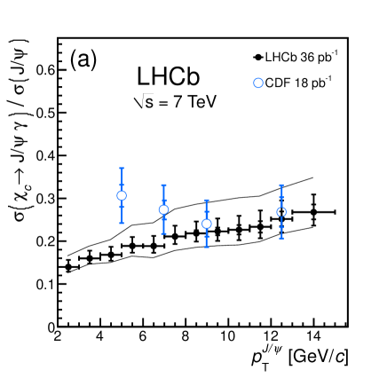
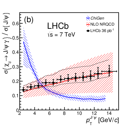
Figure 4: Ratio $\sigma(\chi_{c}\rightarrow{J\mskip-3.0mu/\mskip-2.0mu\psi\mskip 2.0mu}\gamma)\,/\,\sigma({J\mskip-3.0mu/\mskip-2.0mu\psi\mskip 2.0mu})$ in bins of $p_{\mathrm{T}}^{{J\mskip-3.0mu/\mskip-2.0mu\psi\mskip 2.0mu}}$ in the range $2\,{<}\,p_{\mathrm{T}}^{{J\mskip-3.0mu/\mskip-2.0mu\psi\mskip 2.0mu}}\,{<}\,15~{}{\mathrm{\,Ge\kern-0.90005ptV\!/}c}$. The LHCb results, in the rapidity range $2.0\,{<}\,y^{{J\mskip-3.0mu/\mskip-2.0mu\psi\mskip 2.0mu}}\,{<}\,4.5$ and assuming the production of unpolarised ${J\mskip-3.0mu/\mskip-2.0mu\psi\mskip 2.0mu}$ and $\chi_{c}$ mesons, are shown with solid black circles and the internal error bars correspond to the statistical error; the external error bars include the contribution from the systematic uncertainties (apart from the polarisation). The lines surrounding the data points show the maximum effect of the unknown ${J\mskip-3.0mu/\mskip-2.0mu\psi\mskip 2.0mu}$ and $\chi_{c}$ polarisations on the result. The upper and lower limits correspond to the spin states as described in the text. The CDF data points, at $\sqrt{s}\,{=}\,\mbox{${1.8}\>{\mathrm{\,Te\kern-0.90005ptV}}$}$ in $p\bar{p}$ collisions and in the ${J\mskip-3.0mu/\mskip-2.0mu\psi\mskip 2.0mu}$ pseudo-rapidity range $|\eta^{{J\mskip-3.0mu/\mskip-2.0mu\psi\mskip 2.0mu}}|<1.0$, are shown in (a) with open blue circles [5]. The two hatched bands in (b) correspond to the ChiGen Monte Carlo generator prediction [16] and NLO NRQCD [17].

Theory predictions, calculated in the LHCb rapidity range $2.0\,{<}\,y^{{J\mskip-3.0mu/\mskip-2.0mu\psi\mskip 2.0mu}}\,{<}\,4.5$, from the ChiGen Monte Carlo generator [16] and from the NLO NRQCD calculations [17] are shown as hatched bands in Fig. 4(b). The ChiGen Monte Carlo event generator is an implementation of the leading-order colour-singlet model described in Ref. [18]. However, since the colour-singlet model implemented in ChiGen  does not reliably predict the prompt ${J\mskip-3.0mu/\mskip-2.0mu\psi\mskip 2.0mu}$ cross-section, the $\sigma(\chi_{c}\rightarrow{J\mskip-3.0mu/\mskip-2.0mu\psi\mskip 2.0mu}\gamma)\,/\,\sigma({J\mskip-3.0mu/\mskip-2.0mu\psi\mskip 2.0mu})$ prediction uses the ${J\mskip-3.0mu/\mskip-2.0mu\psi\mskip 2.0mu}$ cross-section measurement from Ref. [2] as the denominator in the cross-section ratio.

Figure 4 also shows the maximum effect of the unknown ${J\mskip-3.0mu/\mskip-2.0mu\psi\mskip 2.0mu}$ and $\chi_{c}$  polarisations on the result, shown as lines surrounding the data points. In the first $p_{\mathrm{T}}^{{J\mskip-3.0mu/\mskip-2.0mu\psi\mskip 2.0mu}}$ bin, the upper limit corresponds to a spin state combination $(|m_{\chi_{c1}}|,|m_{\chi_{c2}}|,\lambda_{{J\mskip-3.0mu/\mskip-2.0mu\psi\mskip 2.0mu}})$ equal to $(1,2,-1)$ and the lower limit to $(0,1,1)$. For all subsequent bins, the upper and lower limits correspond to the spin state combinations $(0,2,-1)$ and $(1,0,1)$ respectively.

In summary, the ratio of the $\sigma(\chi_{c}\rightarrow{J\mskip-3.0mu/\mskip-2.0mu\psi\mskip 2.0mu}\gamma)\,/\,\sigma({J\mskip-3.0mu/\mskip-2.0mu\psi\mskip 2.0mu})$ prompt production cross-sections is measured using 36$\mbox{\,pb}^{-1}$ of data collected by LHCb during 2010 at a centre-of-mass energy $\sqrt{s}\,{=}\,\mbox{${7}\>{\mathrm{\,Te\kern-1.00006ptV}}$}$. The results provide a significant statistical improvement compared to previous measurements [4, 5]. The results are in agreement with the NLO NRQCD model [17] over the full range of $p_{\mathrm{T}}^{{J\mskip-3.0mu/\mskip-2.0mu\psi\mskip 2.0mu}}$. However, there is a significant discrepancy compared to the leading-order colour-singlet model described by the ChiGen Monte Carlo generator [16]. At high $p_{\mathrm{T}}^{{J\mskip-3.0mu/\mskip-2.0mu\psi\mskip 2.0mu}}$, NLO corrections fall less slowly with $p_{\mathrm{T}}^{{J\mskip-3.0mu/\mskip-2.0mu\psi\mskip 2.0mu}}$ and become important, it is therefore not unexpected that the model lies below the data. At low $p_{\mathrm{T}}^{{J\mskip-3.0mu/\mskip-2.0mu\psi\mskip 2.0mu}}$, the data appear to put a severe strain on the colour-singlet model.

References

- [1] G. T. Bodwin, E. Braaten, and G. Lepage, Rigorous QCD analysis of inclusive annihilation and production of heavy quarkonium, Phys. Rev. D51 (1995) 1125, arXiv:hep-ph/9407339, Erratum-ibid. D55 (1997) 5853
- [2] LHCb collaboration, R. Aaij et al., Measurement of production in pp collisions at =7 TeV, Eur. Phys. J. C71 (2011) 1645, arXiv:1103.0423
- [3] LHCb collaboration, R. Aaij et al., Measurement of the cross-section ratio for prompt production at TeV, Phys. Lett. B714 (2012) 215, arXiv:1202.1080
- [4] HERA- collaboration, I. Abt et al., Production of the charmonium states and in proton nucleus interactions at = 41.6 GeV, Phys. Rev. D79 (2009) 012001, arXiv:0807.2167
- [5] CDF Collaboration, F. Abe et al., Production of mesons from meson decays in collisions at TeV, Phys. Rev. Lett. 79 (1997) 578
- [6] LHCb collaboration, A. A. Alves Jr et al., The LHCb detector at the LHC, JINST 3 (2008) S08005
- [7] T. Sjöstrand, S. Mrenna, and P. Skands, PYTHIA 6.4 Physics and manual, JHEP 05 (2006) 026, arXiv:hep-ph/0603175
- [8] I. Belyaev et al., Handling of the generation of primary events in Gauss, the LHCb simulation framework, Nuclear Science Symposium Conference Record (NSS/MIC), IEEE (2010) 1155
- [9] D. J. Lange, The EvtGen particle decay simulation package, Nucl. Instrum. Meth. A462 (2001) 152
- [10] E. Barberio and Z. Wa̧s, Photos: a universal Monte Carlo for QED radiative corrections: version 2.0, Comput. Phys. Commun. 79 (1994) 291
- [11] S. Agostinelli et al., Geant4: a simulation toolkit, Nucl. Instrum. Meth. A506 (2003) 250
- [12] Particle Data Group, K. Nakamura et al., Review of particle physics, J. Phys. G37 (2010) 075021, includes 2011 partial update for the 2012 edition.
- [13] T. Skwarnicki, A study of the radiative cascade transitions between the Upsilon-prime and Upsilon resonances. PhD thesis, Institute of Nuclear Physics, Krakow, 1986, DESY-F31-86-02
- [14] BES collaboration, J. Z. Bai et al., decay distributions, Phys. Rev. D62 (2000) 032002, arXiv:hep-ex/9909038
- [15] P. Faccioli and J. Seixas, Observation of and nuclear suppression via dilepton polarization measurements, Phys. Rev. D85 (2012) 074005, arXiv:1203.2033
- [16] L. A. Harland-Lang and W. J. Stirling, http://projects.hepforge.org/superchic/chigen.html
- [17] Y.-Q. Ma, K. Wang, and K.-T. Chao, QCD radiative corrections to production at hadron colliders, Phys. Rev. D83 (2011) 111503, arXiv:1002.3987, calculation in the LHCb rapidity range given by private communication
- [18] E. W. N. Glover, A. D. Martin, and W. J. Stirling, production at large transverse momentum at hadron colliders, Z. Phys. C38 (1988) 473, Erratum-ibid. C49 (1991) 526