On Chubanov’s method for Linear Programming

Abstract

We discuss the method recently proposed by S. Chubanov for the linear feasibility problem. We present new, concise proofs and interpretations of some of his results. We then show how our proofs can be used to find strongly polynomial time algorithms for special classes of linear feasibility problems. Under certain conditions, these results provide new proofs of classical results obtained by Tardos, and Vavasis and Ye.

1 Introduction

In their now classical papers, Agmon [1] and Motzkin and Schoenberg [15] introduced the so called relaxation method to determine the feasibility of a system of linear inequalities (it is well-known that optimization and the feasibility problem are polynomially equivalent to one another). Starting from any initial point, a sequence of points is generated. If the current point $z_{i}$ is feasible we stop, else there must be at least one constraint $c^{T}x\leq d$ that is violated. We will denote the corresponding hyperplane by $(c,d)$. Let $p_{(c,d)}(z_{i})$ be the orthogonal projection of $z_{i}$ onto the hyperplane $(c,d)$, choose a number $\lambda$ (usually chosen between $0$ and $2$), and define the new point $z_{i+1}$ by $z_{i+1}=z_{i}+\lambda(p_{(c,d)}(z_{i})-z_{i})$. Agmon, Motzkin and Schoenberg showed that if the original system of inequalities is feasible, then this procedure generates a sequence of points which converges, in the limit, to a feasible point. So in practice, we stop either when we find a feasible point, or when we are close enough, i.e., any violated constraint is violated by a very small (predetermined) amount.

Many different versions of the relaxation method have been proposed, depending on how the step-length multiplier $\lambda$ is chosen and which violated hyperplane is used. For example, the well-known perceptron algorithms [3] can be thought of as members of this family of methods. In addition to linear programming feasibility, similar iterative ideas have been used in the solution of overdetermined system of linear equations as in the Kaczmarz’s method where iterated projections into hyperplanes are used to generate a solution (see [12, 19, 16]).

The original relaxation method was shown early on to have a poor practical convergence to a solution (and in fact, finiteness could only be proved in some cases), thus relaxation methods took second place behind other techniques for years. During the height of the fame of the ellipsoid method, the relaxation method was revisited with interest because the two algorithms share a lot in common in their structure (see [2, 9, 21] and references therein) with the result that one can show that the relaxation method is finite in all cases when using rational data, and thus can handle infeasible systems. In some special cases the method did give a polynomial time algorithm [14], but in general it was shown to be an exponential time algorithm (see [10, 21]). Most recently in 2004, Betke gave a version that had polynomial guarantee in some cases and reported on experiments [4]. In late 2010 Sergei Chubanov presented a variant of the relaxation algorithm, that was based on the divide-and-conquer paradigm. We will refer to this algorithm as the Chubanov Relaxation algorithm. The purpose of the Chubanov Relaxation algorithm [6] is to either find a solution of

$$\begin{array}[]{l}Ax=b,\\ Cx\leq d\end{array}$$ (1)

in $\mathbb{R}^{n}$, with $A$ an $m\times n$ matrix, $C$ an $l\times n$ matrix, $b\in\mathbb{R}^{m}$, and $d\in\mathbb{R}^{l}$, where the elements of $A$, $b$, $C$, and $d$ are integers, or determine the system has no integer solutions. The advantage of Chubanov’s algorithm is that when the inequalities take the form $\textbf{0}\leq x\leq\textbf{1}$, then the algorithm runs in strongly polynomial time. This result can then be applied to give a new polynomial time algorithm for linear optimization [7]. The purpose of this paper is to investigate these recent ideas in the theory of linear optimization, simplify some of his arguments, and show some consequences.

Our Results

We start by explaining the basic details of Chubanov’s algorithm in Section 2; in particular, we outline the main “Divide and Conquer” subroutine from his paper. We will refer to this subroutine as Chubanov’s D&C algorithm in the rest of the paper. Chubanov’s D&C algorithm is the main ingredient in the Chubanov Relaxation algorithm. In the rest of Section 2, we prove some key lemmas about the D&C algorithm whose content can be summarized in the following theorem.

Theorem 1.1.

Chubanov’s D&C algorithm can be used to infer one of the following statements about the system (1) :

• A feasible solution to (1) exists, and can be found using the output of the D&C algorithm.

• One of the inequalities in $Cx\leq d$ is an implied equality, i.e., there exists $k\in\{1,\ldots,l\}$ such that $c_{k}x=d$ for all solutions to (1).

• There exists $k\in\{1,\ldots,l\}$ such that $c_{k}x=d$ for all integer solutions to (1).

A constructive proof for the above theorem can be obtained using results in Chubanov’s original paper [6]. Our contribution here is to provide a different, albeit existential, proof of this theorem. We feel our proof is more geometric and simpler than Chubanov’s original proof. We hope this will help to expose more clearly the main intuition behind Chubanov’s D&C algorithm, which is the workhorse behind Chubanov’s results. Of course, Chubanov’s constructive proof is more powerful in that it enables him to prove the following fascinating theorem.

Theorem 1.2.

[see Theorem 5.1 in [6]] Chubanov’s Relaxation algorithm either finds a solution to the system

$$\begin{array}[]{l}Ax=b,\\ \mathbf{0}\leq x\leq\mathbf{1},\end{array}$$ (2)

or decides that there are no integer solutions to this system. Moreover, the algorithm runs in strongly polynomial time.

This is an interesting theorem and leads to a new polynomial time algorithm for Linear Programming [7]. However, it suffers from the drawback that it does not lead to a strongly polynomial time linear programming algorithm, even in the restricted setting of variables bounded between 0 and 1. Using the intuition behind our own proofs of Theorem 1.1, we are able to demonstrate how Chubanov’s D&C algorithm can be used to give a strongly polynomial algorithm for deciding the feasibility or infeasibility of a system like (2), under certain additional assumptions. In particular, we show the following result about bounded linear feasibility problems in Section 3.

Theorem 1.3.

Consider the linear program given by

$$\begin{array}[]{l}Ax=b,\\ \mathbf{0}\leq x\leq\lambda\mathbf{1}.\end{array}$$ (3)

Suppose $A$ is a totally unimodular matrix and $\lambda$ is bounded by a polynomial in $n,m$ (the latter happens, for instance, when $\lambda=1$). Furthermore, suppose we know that if (3) is feasible, it has a strictly feasible solution. Then there exists a strongly polynomial time algorithm that either finds a feasible solution of (3), or correctly decides that the system is infeasible. The running time for this algorithm is $O\left(m^{3}+m^{2}n+n^{2}m+n^{2}(2n\lambda\sqrt{2n+1})^{\frac{1}{\log_{2}\left(\frac{7}{5}\right)}}\right)$. If $\lambda=1$, then the running time can be upper bounded by $O(m^{3}+m^{2}n+n^{2}m+n^{5.1})$.

This theorem partially recovers E. Tardos’ result on combinatorial LPs [20]. Tardos’ results were also obtained by Vavasis and Ye using interior point methods [22], which is different from Tardos’ approach. Our Theorem 1.3 proves a weaker version of these classical results using a completely different set of tools, inspired by Chubanov’s ideas. Tardos’ result is much stronger because she does not assume any upper bounds on the variables ($\lambda=\infty$), does not assume strictly feasible solutions, and only assumes that the entries of $A$ are polynomially bounded by $n,m$. Nevertheless our result has some interest as the techniques are completely different from those in [20], [22].

We also show that Chubanov’s D&C subroutine can be used to construct a new algorithm for solving general linear programs. This is completely different from Chubanov’s linear programming algorithm in [7]. However, the general algorithm that we present in this paper is not guaranteed to run in polynomial time. On the other hand, it has the advantage of avoiding some complicated reformulations that Chubanov uses to extract a general purpose LP algorithm from the Chubanov Relaxation algorithm. Moreover, we can solve the problem in a single application of the D&C subroutine, whereas the Chubanov Relaxation algorithm needs multiple applications.

2 Chubanov’s Divide and Conquer Algorithm

In this section we will outline Chubanov’s main subroutines for the D&C algorithm as presented in [6].

First, a couple of assumptions and some notation. We assume the matrices $A$ and $C$ have no zero rows and that $A$ is of full rank. Note if $A$ does not have full rank we can easily transform the system into another, $A^{\prime}x=b^{\prime}$, $Cx\leq d$, such that $A^{\prime}$ has full rank without affecting the set of feasible solutions. Let $a_{i}$ denote the $i$-th row of $A$ and $c_{k}$ denote the $k$-th row of $C$. $P$ will denote the set of feasible solutions of (1). Finally, $B(z,r)$ will denote the open ball centered at $z$ of radius $r$ in $\mathbb{R}^{n}$.

One new idea of Chubanov’s algorithm is its use of new induced inequalities. Unlike Motzkin and Schoenberg [15], who only projected onto the original hyperplanes that describe the polyhedron $P$ (see top of Figure 1), Chubanov constructs new valid inequalities along the way and projects onto them too (bottom part of Figure 1).

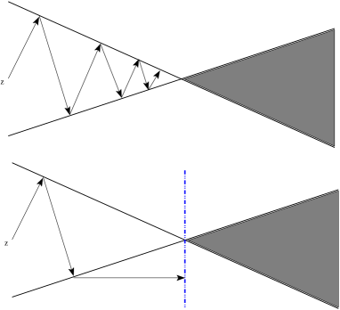
Figure 1: Chubanov’s method generates new inequalities on the way.

The aim of Chubanov’s D&C algorithm is to achieve the following. Given a current guess $z$, a radius $r$ and an error bound $\epsilon>0$, the algorithm will either:

1. Find an $\epsilon$-approximate solution $x^{*}\in B(z,r)$ to (1), i.e. some $x^{*}$ such that

   $$Ax^{*}=b,\ Cx^{*}\leq d+\epsilon\textbf{1},$$

2. Or find an induced hyperplane $hx=\delta$ that separates $B(z,r)$ from $P$.

This task is achieved using a recursive algorithm. In the base case, Chubanov uses a subroutine called Chubanov’s Elementary Procedure (EP), which achieves the above goal if $r$ is small enough; namely, when $r\leq\frac{\epsilon}{2\|c_{\textrm{max}}\|}$, where $\|c_{\textrm{max}}\|=\max_{1\leq k\leq l}(\|c_{k}\|)$. Let $p_{(A,b)}(z)$ denote the projection of $z$ onto the affine subspace defined by $Ax=b$.

Algorithm 2.1.

THE ELEMENTARY PROCEDURE
Input: A system $Ax=b$, $Cx,\leq d$ and the triple $(z,r,\epsilon)$ where $r\leq\frac{\epsilon}{2\|c_{\textrm{max}}\|}$.
Output: Either an $\epsilon$-approximate solution $x^{*}$ or a separating hyperplane $hx=\delta$.

If $\|p_{(A,b)}(z)-z\|<r$ and $\frac{c_{k}z-d_{k}}{\|c_{k}\|}<r$ for all $k$
      Then $x^{*}=p_{(A,b)}(z)$ is an $\epsilon$-approximate solution (see Figure 2)
Else If $\|p_{(A,b)}(z)-z\|\geq r$
      Then let $h=(z-p_{(A,b)}(z))^{T}$ and $\delta=h\cdot p_{(A,b)}(z)$ (see Figure 3)
Else $\frac{c_{k_{0}}z-d_{k_{0}}}{\|c_{k_{0}}\|}\geq r$ for some index $k_{0}$
      Then let $h=c_{k_{0}}$ and $\delta=d_{k_{0}}$ (see Figure 4)
End If

Figure 2: The projection $p(z)$ is an $\epsilon$-approximate solution.

Figure 3: A separating hyperplane is given by the projection direction $(z-p(z))^{T}$.

Figure 4: A separating hyperplane is given by a violated constraint.

Note $\frac{c_{k}z-d_{k}}{\|c_{k}\|}$ tells us how far $z$ is from the hyperplane $c_{k}x=d_{k}$, and it is in fact negative if $z$ satisfies the inequality $c_{k}x\leq d_{k}$. Thus if $\frac{c_{k}z-d_{k}}{\|c_{k}\|}<r$, then any point in $B(z,r)$ is an $\epsilon$-approximation of $c_{k}x\leq d_{k}$. This simple observation is enough to see that the EP procedure solves the task when $r\leq\frac{\epsilon}{2\|c_{\textrm{max}}\|}$. See Chubanov [6] Section 2 for more details and proofs.

The elementary procedure achieves the goal when $r$ is small enough, but what happens when $r>\frac{\epsilon}{2\|c_{\textrm{max}}\|}$? Then the D&C Algorithm makes recursive steps with smaller values of $r$. To complete these recursive steps, the D&C algorithm uses additional projections and separating hyperplanes. We give more details below. Figure 5 illustrates some of the steps in this recursion. A sample recursion tree is shown in Figure 6.

Figure 5: The recursive step in D&C works on two smaller balls with centers $z$ and $z_{0}$

Algorithm 2.2.

THE D&C ALGORITHM
Input: A system $Ax=b$, $Cx\leq d$ and the triple $(z,r,\epsilon)$.
Output: Either an $\epsilon$-approximate solution $x^{*}$, or a separating hyperplane $hx=\delta$.

If $r\leq\frac{\epsilon}{2\|c_{\textrm{max}}\|}$
      Then run the EP on the system
Else recursively run the D&C Algorithm with $(z,\frac{1}{1+\theta}r,\epsilon)$
End If

If the recursive call returns a solution $x^{*}$
      Return $x^{*}$
Else let $h_{1}x=\delta_{1}$ be returned by the recursive call
End If

Set $z_{0}=z-\frac{h_{1}z-\delta_{1}}{h_{1}\cdot h_{1}}\cdot h_{1}$, i.e., project $z$ onto $(h_{1},\delta_{1})$ (see Figure 5)
Run the D&C Algorithm with $(z_{0},\frac{1}{1+\theta}r,\epsilon)$

If the recursive call returns a solution $x^{*}$
      Return $x^{*}$
Else let $h_{2}x=\delta_{2}$ be returned by the recursive call
End If

If $h_{1}=-\gamma h_{2}$ for some $\gamma>0$
      Then STOP, the algorithm fails
Else Find $\alpha$ such that $h=\alpha h_{1}+(1-\alpha)h_{2}$, $\delta=\alpha\delta_{1}+(1-\alpha)\delta_{2}$, and $\frac{hz-\delta}{\|h\|}\geq r$
      Return $hx=\delta$ End If

Figure 6: D&C Recursion Tree

We now state the running time of the Chubanov D&C Algorithm.

Proposition 2.1.

[Theorem 3.1 in [6]] The matrix $A$ is assumed to have $m$ rows and $n$ columns and let $N$ be the number of non-zero entries in the matrix $C$. Let $\mu=\frac{2\epsilon}{28n\lVert c_{max}\rVert^{2}}$ where $c_{max}$ is the row of $C$ with maximum norm. Let $\rho$ be a number such that $|z_{j}|\leq\rho$ and $\rho z_{j}$ is an integer for all components $z_{j}$ of the center $z$ in the input to the D&C algorithm. Let $K=\big{(}\frac{r\lVert c_{max}\rVert}{\epsilon}\big{)}^{\frac{1}{log_{2}(7/5)}}$.

Chubanov’s D&C algorithm performs at most

$$O(m^{3}+m^{2}n+n^{2}m+K\big{(}n\log(\frac{\rho+log(K)(r+n\mu)}{\mu})+n^{2}+N\big{)})$$ (4)

arithmetic operations.

2.1 Using the D&C Algorithm

One possible way to exploit the D&C algorithm is the following. Since D&C returns $\epsilon$-approximate solutions, we can try to run it on the system $Ax=b,Cx\leq d-\epsilon\mathbf{1}$; if the algorithm returns an $\epsilon$-approximate solution, we will have an exact solution for our original system $Ax=b,Cx\leq d$. However, we need a $z$ and an $r$ as input for D&C. To get around this, we can appeal to some results from classical linear programming theory. Suppose one can, a priori, find a real number $r^{*}$ such that if the system $Ax=b,\;Cx\leq d-\epsilon\textbf{1}$ is feasible, then it has a solution with norm at most $r^{*}$. In other words, there exists a solution in $B(0,r^{*})$, if the system is feasible. Such bounds are known in the linear programming literature (see Corollary 10.2b in Schrijver [18]), where $r^{*}$ depends on the entries of $A,b,C,d$ and $\epsilon$. Then one can choose $z=0$ and $r=r^{*}$ for the D&C algorithm. If the algorithm returns an $\epsilon$-approximate solution, we will have an exact solution for our original system $Ax=b,Cx\leq d$; whereas, if the algorithm returns a separating hyerplane, we know that $Ax=b,Cx\leq d-\epsilon\mathbf{1}$ is infeasible by our choice of $r$.

This strategy suffers from three problems.

1. There is a strange outcome in the D&C procedure - when it “fails” and stops. This occurs when the two recursive branches return hyperplanes with normal vectors $h_{1},h_{2}$ with $h_{1}=-\gamma h_{2}$ for some $\gamma>0$. It is not clear what we can learn about the problem from this outcome. Later in this paper, we will interpret this outcome in a manner that is different from Chubanov’s interpretation.

2. It might happen that $Ax=b,Cx\leq d-\epsilon\mathbf{1}$ is infeasible, even if the original system $Ax=b,Cx\leq d$ is feasible. In this case the algorithm may return a separating hyperplane, but we cannot get any information about our original system. All we learn is that $Ax=b,Cx\leq d-\epsilon\mathbf{1}$ is infeasible.

3. Finally, the running time of the D&C algorithm is a polynomial in $n,m$ and $r=r^{*}$. Typically, the classical bounds on $r^{*}$ are exponential in the data. This would mean the running time of the algorithm is not polynomial in the input data.

Let us concentrate on tackling the first two problems, to progress towards a correct linear programming algorithm. Then we can worry about the running time. This requires a second important idea in Chubanov’s work. We address the first two problems above by homogenizing, or parameterizing, our original system, and we show how this helps in the rest of this section. Geometrically this turns the original polyhedron into an unbounded polyhedron, defined by

$$\begin{array}[]{l}Ax-bt=\textbf{0},\\ Cx-dt\leq\textbf{0},\\ -t\leq-1.\end{array}$$ (5)

Note this system (5) is feasible if and only if (1) is feasible. Let $(x^{*},t^{*})$ be a solution to (5). Then $\frac{x^{*}}{t^{*}}$ is a solution of (1). Similarly, if $x^{*}$ is a solution of (1), then $(x^{*},1)$ is a solution of (5). Thus we can apply the D&C to a strengthened parameterized system

$$\begin{array}[]{l}Ax-bt=\textbf{0},\\ Cx-dt\leq-\epsilon\textbf{1},\\ -t\leq-1-\epsilon\end{array}$$ (6)

and any $\epsilon$-approximate solution will be an exact solution of (5), and thus will give us an exact solution of (1). We still need to figure out what $z$ and $r$ to use. For the rest of the paper, we will use $\epsilon=1$ as done by Chubanov in his paper. It turns out that if we choose the appropriate $z$ and $r$, we can get interesting information about the original system $Ax=b,Cx\leq d$ when D&C fails, or returns a separating hyperplane. We explain this next.

Let us summarize before we proceed. Given a system (1) we parameterize and then strengthen with $\epsilon=1$ (to obtain a system in the form (6)). Then we apply the D&C to (6) with appropriately chosen $z$ and $r$. Our three possible outcomes are:

1. The D&C gives us a solution $(x^{*},t^{*})$ which is an $\epsilon=1$-approximate solution to (6). This is the best possible outcome, because we can then return the exact solution $\frac{x^{*}}{t^{*}}$ to (1).

2. The D&C fails. The reader can look ahead to our Proposition 2.4 for an interpretation of this outcome.

3. The D&C returns a separating hyperplane $hx=\delta$. Our Proposition 2.5 tells us how to interpret this outcome.

In the rest of this section, we give some more geometric intuition behind the process of homogenizing the polyhedron and why it is useful. Our goal will be to prove Theorem 1.1.

2.2 Meaning of “Failure” Outcome in D&C

First we show that if the Chubanov D&C algorithm fails on a particular system, then in fact that system is infeasible. This observation is never made in the original paper by Chubanov [6] and, as far as we know, is new.

Proposition 2.2.

Suppose Chubanov’s D&C Algorithm fails on the system $Ax=b,Cx\leq d$, i.e., it returns two hyperplanes $h_{1}x=\delta_{1}$ and $h_{2}x=\delta_{2}$ with $h_{1}=-\gamma h_{2}$ with $\gamma>0$. Then the system $Ax=b,Cx\leq d$ is infeasible.

Proof.

Let $P=\{x\in\mathbb{R}^{n}\mid Ax=b,Cx\leq d\}$. If Chubanov’s algorithm fails, then there exists $z\in\mathbb{R}^{n},r>0$ such that the following two things happen :

1. $h_{1}x\leq\delta_{1}$ is valid for $P$ and for all $y\in B(z,\frac{1}{1+\theta}r)$, $h_{1}y>\delta_{1}$.

2. $h_{2}x\leq\delta_{2}$ is valid for $P$ and for all $y\in B(z_{0},\frac{1}{1+\theta}r)$, $h_{2}y>\delta_{2}$, where $z_{0}=z-\frac{h_{1}z-\delta_{1}}{h_{1}\cdot h_{1}}\cdot h_{1}$.

Since $z_{0}-\frac{r}{2(1+\theta)}\frac{h_{2}}{\lVert h_{2}\rVert}\in B(z_{0},\frac{1}{1+\theta}r)$, $h_{2}\cdot(z_{0}-\frac{r}{2(1+\theta)}\frac{h_{2}}{\lVert h_{2}\rVert})>\delta_{1}$. Therefore,

$$h_{2}z_{0}-\frac{r\lVert h_{2}\rVert}{2(1+\theta)}>\delta_{2}.$$ (7)

Now we use the fact that $h_{1}=-\gamma h_{2}$ and so $-\frac{1}{\gamma}h_{1}=h_{2}$ which we substitute into (7) to get $-\frac{1}{\gamma}h_{1}z_{0}-\frac{r\lVert h_{2}\rVert}{2(1+\theta)}>\delta_{2}$. From the definition of $z_{0}$, we have $h_{1}z_{0}=\delta_{1}$. Therefore, $-\frac{1}{\gamma}\delta_{1}>\frac{r\lVert h_{2}\rVert}{2(1+\theta)}+\delta_{2}>\delta_{2}$. So $\delta_{1}<-\gamma\delta_{2}$. Now $h_{1}x\leq\delta_{1}$ is valid for $P$ using (i) above. Using $h_{1}=-\gamma h_{2}$ and $\delta_{1}<-\gamma\delta_{2}$, we get $-\gamma h_{2}x<-\gamma\delta_{2}$ is valid for $P$, i.e., $h_{2}x>\delta_{2}$ is valid for $P$. But we also know that $h_{2}x\leq\delta_{2}$ is valid for $P$ from (ii) above. This implies that $P=\emptyset$ and the system $Ax=b,Cx\leq d$ is infeasible.∎

We now interpret the “failure” outcome of the D&C algorithm on the strengthened parameterized system. First we prove the following useful lemma.

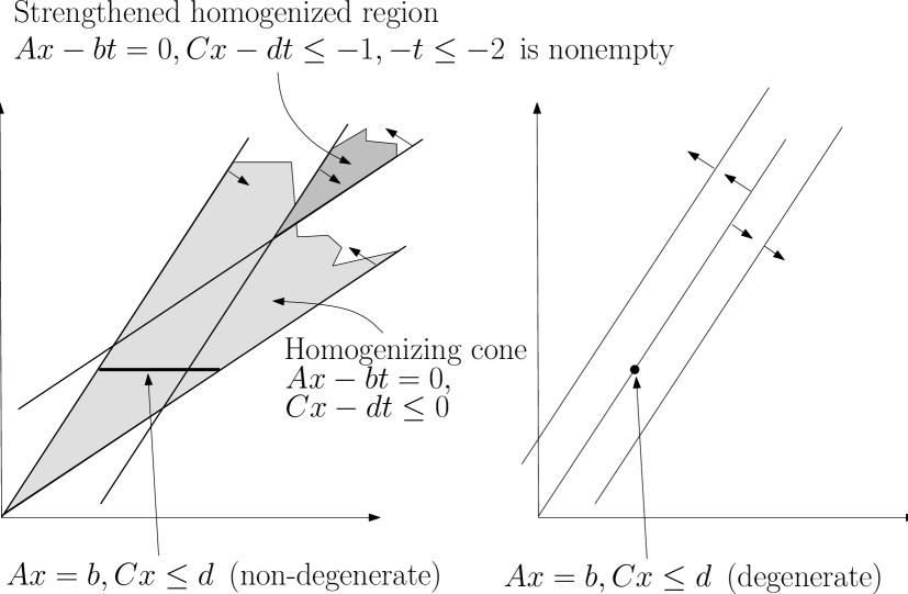
Figure 7: This Figure illustrates our Lemma 2.3. In the left figure, the original feasible region is non-degenerate and so the strengthened, homogenized cone is nonempty. The figure on the right shows an example where the original system is degenerate; the strengthened cone is empty because we have two parallel hyperplanes which get pushed away from each other, creating infeasibility in the strengthened system.

Lemma 2.3.

If the system $Ax-bt=0,Cx-dt\leq-1,-t\leq-2$ is infeasible, then there exists $l\in\{1,\ldots,k\}$ such that $c_{l}\cdot x=d_{l}$ for all $x$ satisfying $Ax=b,Cx\leq d$.

Proof.

We prove the contrapositive. So suppose that for all $k\in\{1,\ldots,l\}$, there exists $x_{k}$ satisfying $Ax_{k}=b,Cx_{k}\leq d$ with $c_{k}\cdot x_{k}<d_{k}$. Then using $\bar{x}=\frac{1}{l}(x_{1}+\ldots+x_{l})$, we get that $A\bar{x}=b$ and $c_{k}\bar{x}<d_{k}$ for all $k\in\{1,\ldots,l\}$. Let $\eta_{k}=d_{k}-c_{k}\cdot\bar{x}>0$ and let $\eta=\min\{\frac{1}{2},\eta_{1},\ldots,\eta_{l}\}$. Therefore, $\eta>0$. Let $x^{*}=\frac{\bar{x}}{\eta}$ and $t^{*}=\frac{1}{\eta}$. Then

$$Ax^{*}-bt^{*}=\frac{1}{\eta}(A\bar{x}-b)=0.$$

For every $k\in\{1,\ldots,l\}$,

$$d_{k}t^{*}-c_{k}x^{*}=\frac{1}{\eta}(d_{k}-c_{k}\bar{x})=\frac{\eta_{k}}{\eta}\geq 1.$$

Therefore, $c_{k}x^{*}-d_{k}t^{*}\leq-1$ for every $k\in\{1,\ldots,l\}$. Finally, since $t=\frac{1}{\eta}\geq 2$ by definition of $\eta$, we have $-t\leq-2$. ∎

An illustration of the above lemma appears in Figure 7. The following is the important conclusion one makes if the D&C algorithm “fails” on the strengthened parameterized system.

Proposition 2.4.

If Chubanov’s D&C algorithm fails on the system $Ax-bt=0,Cx-dt\leq-1,-t\leq-2$, then there exists $l\in\{1,\ldots,k\}$ such that $c_{l}\cdot x=d_{l}$ for all $x$ satisfying $Ax=b,Cx\leq d$.

Proof.

Follows from Proposition 2.2 and Lemma 2.3.∎

2.3 The meaning of when a separating hyperplane is returned by D&C

We now make the second useful observation about the strengthened parameterized system $Ax-bt=0,Cx-dt\leq-1,-t\leq-2$. Suppose we know that all solutions to $Ax=b,Cx\leq d$ have norm at most $r^{*}$. Then we will show that if all solutions to the strengthened system are “too far” from the origin, then the original system is “very thin” (this intuition is illustrated in Figure 8). More precisely, we show that if all solutions to the strengthened parameterized system have norm greater than $2k(r^{*}+1)$, then there exists an inequality $c_{l}x\leq d_{l}$ such that all solutions to $Ax=b,Cx\leq d$ satisfy $d_{l}-\frac{1}{2}\leq c_{l}x$. That is, the original polyhedron lies in a “thin strip” $d_{l}-\frac{1}{2}\leq c_{l}x\leq d_{l}$. This would then imply that all integer solutions to $Ax=b,Cx\leq d$ satisfy $c_{l}x=d_{l}$ since $c_{l},d_{l}$ have integer entries. Here is the precise statement of this observation.

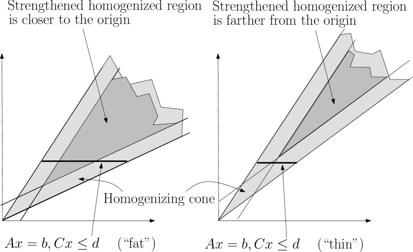
Figure 8: This Figure illustrates our Proposition 2.5. When the original feasible region is “thinner”, the strengthened homogenized cone is pushed farther away from the origin.

Proposition 2.5.

Suppose $r^{*}\in\mathbb{R}$ is such that $\lVert x\rVert\leq r^{*}$ for all $x$ satisfying $Ax=b,Cx\leq d$. If $\lVert(x,t)\rVert>2k(r^{*}+1)$ for all $(x,t)$ satisfying $Ax-bt=0,Cx-dt\leq-1,-t\leq-2$, then there exists $l\in\{1,\ldots,k\}$ such that $d_{l}-\frac{1}{2}\leq c_{l}x\leq d_{l}$ for all $x$ satisfying $Ax=b,Cx\leq d$.

Proof.

Suppose to the contrary that for all $j\in\{1,\ldots,k\}$, there exists $x^{j}$ such that $Ax^{j}=b,Cx^{j}\leq d$, and $c_{j}x^{j}\leq d^{j}-\frac{1}{2}$, i.e., $c_{j}(2x^{j})-2d_{j}\leq-1$. This implies that the following equations hold for all $j\in\{1,\ldots,k\}$

$$\begin{array}[]{l}c_{j}(2x^{j})-2d_{j}\leq-1,\\ c_{j}(2x^{i})-2d_{j}\leq 0\qquad\forall i\neq j.\end{array}$$ (8)

Now consider $\hat{x}=\sum_{j=1}^{k}2x^{j}$ and $\hat{t}=2k$. It is easily verified $A\hat{x}-b\hat{t}=0$ since $Ax^{j}=b$ for all $j\in\{1,\ldots,k\}$. Moreover, adding together the inequalities in (8), we get that $c_{j}\hat{x}-d_{j}\hat{t}\leq-1$ for all $j\in\{1,\ldots,k\}$. Therefore, $(\hat{x},\hat{t})$ satisfies the constraints $Ax-bt=0,Cx-dt\leq-1,-t\leq-2$.

Finally, $\lVert(\hat{x},\hat{t})\rVert\leq\lVert\hat{x}\rVert+2k\leq\sum_{j=1}^{k}2\lVert x^{j}\rVert+2k\leq 2k(r^{*}+1)$, where the last inequality follows from the fact that all solutions to $Ax=b,Cx\leq d$ have norm at most $r^{*}$. We have thus reached a contradiction with the hypothesis that $\lVert(x,t)\rVert>2k(r^{*}+1)$ for all $(x,t)$ satisfying $Ax-bt=0,Cx-dt\leq-1,-t\leq-2$.∎

The above proposition shows that if Chubanov’s D&C algorithm returns a separating hyperplane separating the feasible region of $Ax-bt=0,Cx-dt\leq-1,-t\leq-2$ from the ball $B(0,2k(r^{*}+1))$, one can infer that there exists an inequality $c_{l}x\leq d_{l}$ that is satisfied at equality by all integer solutions to $Ax=b,Cx\leq d$.

We now have all the tools to prove Theorem 1.1.

Proof of Theorem 1.1.

As discussed earlier, we can assume that there exists $r^{*}$ such that $\lVert x\rVert\leq r^{*}$ for all $x$ satisfying $Ax=b,Cx\leq d$. We then run the D&C algorithm on the strengthened system (6) with $\epsilon=1$, $z=0$ and $r=2k(r^{*}+1)$. Recall the three possible outcomes of this algorithm. In the first outcome, we can find an exact solution of $Ax=b,Cx\leq d$ - this is (i) in the statement of the theorem. In the second outcome, when D&C fails, Proposition 2.4 tells that we have an implied equality, which is (ii) in the statement of the theorem. Finally, in the third outcome, D&C returns a separating hyperplane. By Proposition 2.5, we know that there exists an inequality $c_{l}x\leq d_{l}$ that is satisfied at equality by all integer solutions to $Ax=b,Cx\leq d$. This is (iii) in the statement of the theorem. ∎

2.4 Chubanov’s proof of Theorem 1.2

Chubanov is able to convert the existential results of Propositions 2.4 and 2.5 into constructive procedures, wherein he can find the corresponding implied equalities in strongly polynomial time. He then proceeds to apply the D&C procedure iteratively and reduce the number of inequalities by one at every iteration. One needs at most $l$ such iterations and at the end one is left with a system of equations. This system can be tested for feasibility in strongly polynomial time by standard linear algebraic procedures. This is the main idea behind the Chubanov Relaxation algorithm and the proof of Theorem 1.2 that appears in [6].

3 Linear feasibility problems with strictly feasible solutions

We will now demonstrate that using the lemmas we proved in Section 2, we can actually give strongly polynomial time algorithms for certain classes of linear feasibility problems. More concretely, we aim to prove Theorem 1.3. Consider a linear feability problem in the following standard form.

$$\begin{array}[]{l}Ax=b,\\ -x\leq\textbf{0},\end{array}$$ (9)

where $A\in\mathbb{R}^{m\times n}$ and $b\in\mathbb{R}^{m}$. We will assume that the entries of $A$ and $b$ are integers and that $A$ has full row rank. Let

$$\Delta_{A}=\max\{|det(B)|\mid B\textrm{ is an }n\times n\textrm{ submatrix of }A\}$$

be the maximum subdeterminant of the matrix $A$. Let $P(A,b)=\{x\in\mathbb{R}^{n}\mid Ax=b,-x\leq\textbf{0}\}$ denote the feasible region of (9).

Lemma 3.1.

Let $x$ be any vertex of $P(A,b)$. If $x_{i}>0$ for some $i\in\{1,\ldots,n\}$, then $x_{i}\geq\frac{1}{\Delta_{A}}$.

Proof.

Since $x$ is a vertex, there exists a nonsingular $n\times n$ submatrix $B$ of $A$ such that $x$ is the basic feasible solution corresponding to the basis $B$. That is, the non basic variables are $0$ and the basic variable values are given in the vector $B^{-1}b$. If for some $i$, $x_{i}>0$ then this is a basic variable and therefore its value is at least $\frac{1}{|det(B)|}$ since $b$ is an integer vector. Since $|det(B)|\leq\Delta_{A}$, we have that $x_{i}\geq\frac{1}{\Delta_{A}}$. ∎

Lemma 3.2.

Suppose we know that (9) has a strictly feasible solution, i.e. there exists $\bar{x}\in\mathbb{R}^{n}$ such that $A\bar{x}=b$ and $\bar{x}_{i}>0$ for all $i\in\{1,\ldots,n\}$. If $P(A,b)$ is bounded, then there exists a solution $x^{*}\in\mathbb{R}^{n}$ such that $Ax^{*}=b$ and $x^{*}_{i}\geq\frac{1}{n\Delta_{A}}$ for all $i\in\{1,\ldots,n\}$.

Proof.

Since we have a strictly feasible solution and $P(A,b)$ is a polytope, then for every $i\in\{1,\ldots,n\}$ there exists a vertex $\bar{x}^{i}$ of $P$ such that $\bar{x}^{i}_{i}>0$. By Lemma 3.1, we have that $\bar{x}^{i}_{i}\geq\frac{1}{\Delta_{A}}$. Therefore, if we consider the solution

$$x^{*}=\frac{1}{n}\sum_{i=1}^{n}\bar{x}^{i},$$

i.e., the convex hull of all these $n$ vertices, then $x^{*}_{i}\geq\frac{1}{n\Delta_{A}}$ for all $i\in\{1,\ldots,n\}$. ∎

We now consider linear feasibility problems of the form (9) such that either it is infeasible or has a strictly feasible solution. We will present an algorithm to decide if such linear feasibility problems are feasible or infeasible. We call this algorithm the LFS Algorithm, as an acronym for Linear Feasibility problems with Strict solutions. As part of the input, we will take $\Delta_{A}$, as well as a real number $r$ such that $P(A,b)\subset B(0,r)$, i.e., $\lVert x\rVert<r$ for all feasible solutions $x$. The running time of our algorithm will depend on $\Delta_{A},r$, and $n$.

Algorithm 3.1.

THE LFS ALGORITHM
Input: $Ax=b$, $-x\leq\textbf{0}$, such that either this system is infeasible, or there exists a strictly feasible solution. We are also given a real number $r$ such that $P(A,b)\subset B(0,r)$, i.e., $\lVert x\rVert<r$ for all feasible solutions $x$. Moreover, we are given $\Delta_{A}$ as part of the input.
Output: A feasible point $x^{*}$ or the decision that the system is infeasible.
Parameterize (9):

$$\begin{array}[]{l}Ax-bt=0,\\ -x\leq 0,\\ -t\leq-1.\end{array}$$ (10)

Run Chubanov’s D&C subroutine on the strengthened version of (10):

$$\begin{array}[]{l}Ax-bt=0,\\ -x\leq-1,\\ -t\leq-2.\end{array}$$ (11)

with $z=\textbf{0}$, $\hat{r}=2n\Delta_{A}\sqrt{r^{2}+1}$, and $\epsilon=1$
If Chubanov’s D&C subroutine finds an $\epsilon$-feasible solution $(x^{*},t^{*})$
      Return $\hat{x}=\frac{x^{*}}{t^{*}}$ as a feasible solution for (9).
Else (Chubanov’s D&C subroutine fails or returns a separating hyperplane)
      Return “The system (9) is INFEASIBLE”

Theorem 3.3.

The LFS Algorithm correctly determines a feasible point $x^{*}$ of (9) or determines the system is infeasible. The running time is

$$O\left(m^{3}+m^{2}n+n^{2}m+(2n\Delta_{A}\sqrt{r^{2}+1})^{\frac{1}{\log_{2}\left(\frac{7}{5}\right)}}\left(n^{2}+n\log\Delta_{A}+n\log(r)\right)\right)$$

Proof.

We first confirm the running time. We will use Proposition 2.1. Observe that for our input to the D&C algorithm, $\lVert c_{max}\rVert=1$, $\epsilon=1$ and $\hat{r}=2n\Delta_{A}\sqrt{r^{2}+1}$ and $N=n$. Therefore, $K=(2n\Delta_{A}\sqrt{r^{2}+1})^{\frac{1}{\log_{2}\left(\frac{7}{5}\right)}}$, $\rho=0$ since we use the origin as the initial center for the D&C algorithm, $\mu=\frac{1}{14n}$. Substituting this into (4), we get the stated running time for the LFS algorithm.

To prove the correctness of the algorithm, we need to look at each of the three cases Chubanov’s D&C can return.

CASE 1: An $\epsilon$-approximate solution $(x^{*},t^{*})$ is found for (17). Then $(x^{*},t^{*})$ is an exact solution to (10), and $\frac{x^{*}}{t^{*}}$ is a solution to (9).

CASE 2: The D&C algorithm fails to complete, returning consecutive separating hyperplanes $(h_{1},\delta_{1})$ and $(h_{2},\delta_{2})$ such that $h_{1}=-\gamma h_{2}$ for some $\gamma>0$. Then Proposition 2.4 says that there exists $i\in\{1,\ldots,n\}$ such that $x_{i}=0$ for all feasible solutions to (9). But then the original system (9) has no strictly feasible solution, and by our assumption, is therefore actually infeasible. Therefore if the D&C fails, our original system $Ax=b$, $-x\leq\textbf{0}$ is infeasible.
CASE 3: The final case is when the D&C algorithm returns a separating hyperplane $(h,\delta)$, separating $B(0,\hat{r})$ from the feasible set of (11). We now show that this implies the original system $Ax=b$, $-x\leq\textbf{0}$ is infeasible.

If not, then from our assumption, we have a strictly feasible solution $x^{*}$ for (9). By Lemma 3.2, we know that $x^{*}_{i}\geq\frac{1}{n\Delta_{A}}$ for all $i\in\{1,\ldots,n\}$. Consider the point $(\bar{x},\bar{t})=(2n\Delta_{A}x^{*},2n\Delta_{A})$ in $\mathbb{R}^{n+1}$. We show that $(\bar{x},\bar{t})$ is feasible to (11). Since $Ax^{*}=b$, we have that $A\bar{x}-b\bar{t}=0$. Moreover, since $x^{*}_{i}\geq\frac{1}{n\Delta_{A}}$ for all $i\in\{1,\ldots,n\}$, we have that $\bar{x}=2n\Delta_{A}x^{*}\geq\textbf{1}$, i.e., $-\bar{x}\leq-1$. Finally, $\bar{t}=2n\Delta_{A}\geq 2$, since $\Delta_{A}\geq 1$ and $n\geq 1$. Therefore, $-\bar{t}\leq-2$. Now we check the norm of this point $\lVert(\bar{x},\bar{t})\rVert=\lVert(2n\Delta_{A}x^{*},2n\Delta_{A})\rVert=2n\Delta_{A}\lVert(x^{*},1)\rVert$. Since $x^{*}\in P(A,b)\subset B(0,r)$, we know that $\lVert x^{*}\rVert<r$. Therefore, $\lVert(\bar{x},\bar{t})\rVert<\hat{r}$. So $(\bar{x},\bar{t})$ is a feasible solution to (11) and $(\bar{x},\bar{t})\in B(0,\hat{r})$. But D&C returned a separating hyperplane separating $B(0,\hat{r})$ from the feasible set of (11). This is a contradiction. Hence, we conclude that $Ax=b$, $-x\leq\textbf{0}$ is infeasible. ∎

Corollary 3.4.

Consider the following system.

$$\begin{array}[]{l}Ax=b,\\ \textbf{0}\leq x\leq\lambda\textbf{1}.\end{array}$$ (12)

Suppose that we know that the above system is either infeasible, or has a strictly feasible solution, i.e., there exists $\bar{x}$ such that $A\bar{x}=b$ and $\textbf{0}<\bar{x}<\lambda\textbf{1}$. Then there exists an algorithm which either returns a feasible solution to (12), or correctly decides that the system is infeasible, with running time

$$O\left(m^{3}+m^{2}n+n^{2}m+(2n\Delta_{A}\lambda\sqrt{2n+1})^{\frac{1}{\log_{2}\left(\frac{7}{5}\right)}}\left(n^{2}+n\log\Delta_{A}+n\log(\lambda)\right)\right).$$

Proof.

We first put (12) a standard form.

$$\begin{array}[]{l}Ax=b,\\ x+y=\lambda\textbf{1},\\ -x\leq\textbf{0},\\ -y\leq\textbf{0}.\end{array}$$ (13)

We will use the constraint matrix of (13) :

$$\tilde{A}=\left[\begin{array}[]{cc}A&\mathbf{0}_{m\times n}\\ I_{n}&I_{n}\end{array}\right],$$

where $\mathbf{0}_{m\times n}$ denotes the $m\times n$ matrix with all 0 entires, and $I_{n}$ is the $n\times n$ identity matrix. Therefore, $P(\tilde{A},[b,\lambda\textbf{1}])$ is the feasible set for (13). Also, note that $\Delta_{\tilde{A}}=\Delta_{A}$. Since $\textbf{0}\leq x,y\leq\lambda\textbf{1}$ for all $(x,y)\in P(\tilde{A},[b,\lambda\textbf{1}])$, we know that $P(\tilde{A},[b,\textbf{1}])\subset B(0,\lambda\sqrt{2n})$. Therefore, we run LFS with $r=\lambda\sqrt{2n}$ and the system (13) as input. Observe that since (12) has a strictly feasible solution, so does (13). By Theorem 3.3, LFS either returns a feasible solution to (13) which immediately gives a feasible solution to (12), or correctly decides that (13) is infeasible and hence (12) is infeasible. Moreover, the running time for LFS is

$$\begin{array}[]{c}O\left((m^{3}+m^{2}n+n^{2}m+(2n\Delta\sqrt{r^{2}+1})^{\frac{1}{\log_{2}\left(\frac{7}{5}\right)}}\left(n^{2}+n\log\Delta_{A}+n\log(r)\right)\right)\\ =O\left(m^{3}+m^{2}n+n^{2}m+(2n\Delta_{A}\lambda\sqrt{2n+1})^{\frac{1}{\log_{2}\left(\frac{7}{5}\right)}}\left(n^{2}+n\log\Delta_{A}+n\log(\lambda)\right)\right).\end{array}$$

∎

Corollary 3.4 is related to the following theorem of Schrijver. Let $\tilde{\Delta}_{A}=\max\{|det(B^{-1})|\mid B\textrm{ is a nonsingular submatrix of A}\}$.

Theorem 3.5 (Theorem 12.3 in [18]).

A combination of the relaxation method and the simultaneous diophantine approximation method solves a system $Ax\leq b$ of rational linear inequalities in time polynomially bounded by $size(A,b)$ and by $\tilde{\Delta}_{A}$.

On one hand, we have the additional assumptions of being bounded and having strictly feasible solutions. On the other hand, we can get rid of the dependence of the running time on $size(A,b)$ and the use of the simultaneous diophantine approximation method, which utilizes non-trivial lattice algorithms. It is also not immediately clear how $\Delta_{A}$ is related to $\tilde{\Delta}_{A}$. We finally prove Theorem 1.3.

Proof of Theorem 1.3.

If $A$ is totally unimodular, then $\Delta_{A}=1$. The result now follows from Corollary 3.4.∎

4 A General Algorithm for Linear Feasibility Problems

In this section, we describe an algorithm for solving general linear feasibility problems using Chubanov’s D&C algorithm and the ideas developed in Section 2. We call this algorithm the LFG Algorithm, as an acronym for Linear Feasibility problems in General. Before we can state our algorithm and prove its correctness, we need a couple of other pieces.

Lemma 4.1.

[Schrijver Corollary 10.2b] Let $P$ be a rational polyhedron in $\mathbb{R}^{n}$ of facet complexity $\phi$. Define

$$Q=P\cap\{x\in\mathbb{R}^{n}|-2^{5n^{2}\phi}\leq x_{i}\leq 2^{5n^{2}\phi}\ \textrm{for}\ i=1,\ldots,n\}.$$

Then dim$(P)$ = dim$(Q)$.

Thus, if we use $\hat{r}=2^{5n^{2}\phi}\sqrt{n}$ then $B(\textbf{0},\hat{r})$ will circumscribe the hypercube in the above lemma from Schrijver. We will also have dim$(P)$ = dim$(P\cap B(\textbf{0},\hat{r}))$.

The second piece we need comes from Papadimitriou and Stieglitz [17]. Simply put, the theorem states that (1) is feasible if and only if some other system is strictly feasible (i.e. all the inequalities are strict inequalities). The lemma stated below is a stronger version of their Lemma 8.7 in [17].

Lemma 4.2.

[Lemma 8.7 in [17]] The system (1) is feasible if and only if

$$\begin{array}[]{l}Ax=b,\\ Cx<d+\nu.\\ \end{array}$$ (14)

is feasible, where $\nu=2^{-2T}$ when $T$ is the size of the input data. Moreover, given a solution to (14), we can construct a solution to (1) in strongly polynomial time.

Algorithm 4.1.

THE LFG ALGORITHM
Input: $Ax=b$, $-x\leq 0$.
Output: A feasible point $x^{*}$ or the decision the system is infeasible.
Set $\nu=2^{-2T}$ where $T$ is the bit length of the input data
Set a new system

$$\begin{array}[]{l}Ax=b,\\ Cx\leq d+\frac{\nu}{2}.\end{array}$$ (15)

Parameterize (15):

$$\begin{array}[]{l}Ax-bt=0,\\ Cx-(d+\frac{\nu}{2})t\leq 0,\\ -t\leq-1.\end{array}$$ (16)

Run Chubanov’s D&C subroutine on the strengthened version of (16)

$$\begin{array}[]{l}Ax-bt=0,\\ Cx-(d+\frac{\nu}{2})t\leq-1,\\ -t\leq-2.\end{array}$$ (17)

with $z=\textbf{0}$, $r=\hat{r}$ from Lemma 3.2 applied to (17), and $\epsilon=1$
If a feasible solution $(x^{*},t^{*})$ is found
      Return $\hat{x}$ from the proof of Lemma 3.3, with $x_{0}=\frac{x^{*}}{t^{*}}$
Else Lemma 3.1 implies one of our inequalities is an implied equality
      Return “The system (15) is INFEASIBLE”

Theorem 4.3.

The LFG Algorithm correctly determines a feasible point $x^{*}$ of (1) or determines the system is infeasible in a finite number of steps.

Proof.

To prove the correctness of the algorithm, we need to look at each of the three cases Chubanov’s D&C can return.
CASE 1: An $\epsilon$-approximate solution $(x^{*},t^{*})$ is found for (17). Then $(x^{*},t^{*})$ is an exact solution to (16), and $\frac{x^{*}}{t^{*}}$ is a solution to (15), and hence is also a solution to (14). Using Lemma 4.2, we can construct a feasible solution to our original system (1).
CASE 2: The D&C algorithm fails to complete, returning consecutive separating hyperplanes $(h_{1},\delta_{1})$ and $(h_{2},\delta_{2})$ such that $h_{1}=-\gamma h_{2}$ for some $\gamma>0$. By Proposition 2.4, we know that there exists $k\in\{1,\ldots,l\}$ such that $c_{k}x=d_{l}+\frac{\nu}{2}$ for all solutions to $Ax=b,Cx\leq d+\frac{\nu}{2}$. But this simply implies that $Ax=b,Cx\leq d$ is infeasible.
CASE 3: The final case is when the D&C returns a separating hyperplane $(h,\delta)$. Note that due to the $\hat{r}$ we use, this already implies (17) is infeasible. Then by Lemma 2.3, we know there exists some $l$ such that $c_{l}x=d_{l}+\frac{\nu}{2}$ for all $x$ satisfying $Ax=b,Cx\leq d+\frac{\nu}{2}$. Again, as in Case 2, this implies that $Ax=b$, $Cx\leq d$ is infeasible.∎

Since the running time of the D&C subroutine is a polynomial in $\hat{r}$, and $\hat{r}$ is exponential in the input data, our algorithm is not guaranteed to run in polynomial time. However, as mentioned in the Introduction, it has certain advantages over Chubanov’s polynomial time LP algorithm from [7]. Firstly, it avoids the complicated reformulations used by Chubanov, which can potentially cause the actual runtime of his algorithm to be bad in practice. Secondly, the Chubanov Relaxation algorithm requires multiple iterations of the D&C subroutine, whereas the LFG algorithm uses only one application of the D&C subroutine.

5 Computational Experiments

In this final section, we investigate the computational performance of the various relaxation methods mentioned in the preceding sections. We used MATLAB to implement the following algorithms.

1. The Chubanov D&C algorithm, as described in Section 2. We use this algorithm on linear feasibility problems in the following way. We choose $z=0$, $\epsilon=1\times 10^{-6}$ and $r$ is taken as $\sqrt{n+1}$ for binary problems, and it is taken as the input dependent bound given in Lemma 4.1. This would mean that when the algorithm terminates, we either have an $\epsilon$-approximate solution, or we conclude that the system is infeasible.

2. The Chubanov Relaxation algorithm, as described in [6]. Apart from the input data $A,b,C,d$, this algorithm requires as input a real number $r$ such that the feasible region is contained in $B(0,r)$. As with the Chubanov D&C algorithm above, $r$ is taken as $\sqrt{n+1}$ for binary problems, and it is taken as the input dependent bound given in Lemma 4.1 for general linear feasibility.

3. The LFS algorithm, as described in Section 3. This algorithm also requires as input a real number $r$ such that the feasible region is contained in $B(0,r)$. As with the Chubanov D&C algorithm above, $r$ is taken as $\sqrt{n+1}$ for binary problems, and it is taken as the input dependent bound given in Lemma 4.1 for general linear feasibility problems. Moreover, we require as input $\Delta_{A}$, the maximum subdeterminant of the matrix $A$. We use the standard bound $\Delta_{A}\leq n^{\frac{n}{2}}|a_{max}|^{n}$, where $a_{max}$ is the entry of $A$ with largest absolute value.

4. Two versions of the original relaxation algorithm developed by Agmon [1], and Motzkin and Schoenberg [15].

Recall that the Chubanov Relaxation algorithm is not really a linear feasibility algorithm; it may sometimes report that the solution has no integer solutions (see the statement of Theorem 1.2). However, we feel it is still interesting to study its practical run time, and compare it with our linear feasibility algorithms which are also based on the Chubanov D&C algorithm.

It has already been shown that, for most purposes, the original relaxation method is not able to compete with other linear programming algorithms [10, 21]. Thus, the purpose of these experiments is not to compare the running times with current commercial software. Rather, we want to determine how the new relaxation-type algorithms, based on the Chubanov D&C algorithm, compare with the original relaxation algorithm suggested by Agmon, and Motzkin and Schoenberg. Despite the improved theoretical performance of the new algorithms, the tables below show that, in practice, the original relaxation method is by far the preferred method in almost every case.

As noted above, the algorithms and experiment scripts were all developed in MATLAB 7.12.0. No parallelization was incorporated into the algorithms. The computational experiments were run on a personal computer with an Intel Core i5 M560 2.67 GHz processor. The problems used were drawn from the Netlib repository [8], the MIPLIB repository [5, 13], Hoffman’s experiments [11], Telgen’s and Goffin’s example [10, 21] which shows the exponential behavior of the original relaxation method, and some randomly generated problems. The code and the problems used are available at http://www.math.ucdavis.edu/$\sim$mjunod/.

In every table, a dash “–” denotes an experiment that exceeded our default time limit of 10 minutes. For example, in Table 1 Chubanov’s algorithm timed out on the third Telgen experiment. Given the size and complexity of the problems involved, we determined that any algorithm exceeding 10 minutes had already shown how practically inefficient it was for that problem. When all of the algorithms timed out on a single problem, the results for the problem are not reported in the tables. We note here that for some experiments we rely on some familiarity with the problem and determine our own bound for $r$ in the algorithms, to speed up the computations. All of the run times reported are in seconds.

We note here that our LFS algorithm timed out on all instances tried. The Chubanov Relaxation algorithm and the Chubanov D&C algorithms timed out on all Netlib and MIPLIB problems, as well as on all the problems from Hoffman’s experiments. Hence, the LFS algorithm is not reported in any table. Results for the Chubanov Relaxation algorithm and the Chubanov D&C algorithms on the Telgen examples are reported in Table 1, and their results on the random $0-1$ instances are reported in Table 3.

Table 1: Telgen Results for the Chubanov Relaxation Algorithm and the Chubanov D&C Algorithm

	Chubanov Relaxation		Chubanov D&C
Experiment	Recursions	Time	Recursions	Time
		(Sec)		(Sec)
Telgen ($\alpha=1$)	139254	30.4761	51	0.0010
Telgen ($\alpha=2$)	$2.12991\times 10^{6}$	451.817	109	0.0177
Telgen ($\alpha=3$)	–	–	116	0.0211
Telgen ($\alpha=4$)	–	–	124	0.0169
Telgen ($\alpha=5$)	–	–	132	0.0218

Table 2 compares two variants of the original relaxation method. The two versions of the original relaxation method differ only in how the violated constraint is chosen. See [1, 15] for a full explanation of the algorithm. In the first implementation, called “Regular” in the tables, we chose the maximally violated constraint as specified by Agmon, and Motzkin and Schoenberg. Our second implementation, called “Random” in the tables, randomly chooses a violated constraint to see if there is any practical gain, as Needell’s paper on the Kaczmarz method [16] suggests might be possible. Every time we ran the “Random” version on a problem, we ran it 100 times and we are reporting the average number of iterations, time in seconds, and the standard deviation of each data set. In the experiments labeled Telgen, only two constraints exist in the problem and only one is violated at any iteration. Thus only the “Regular” version is reported as the two gave identical results. For every experiment we set $\lambda=1.9$ as a higher over-projection constant increases the speed of convergence, and let $\epsilon=1\times 10^{-6}$ be our error constant.

Table 3 compares the performance of the Chubanov Relaxation algorithm, the Chubanov D&C algorithm and the original relaxation algorithm, on the randomly generated 0-1 problem set. These were problems of the form $Ax=b$, $\textbf{0}\leq x\leq\textbf{1}$ with the dimension noted in each row. We limited ourselves to a randomly generated 0-1 matrix $A$ with anywhere from 1 to $n-1$ rows, also randomly chosen, and populated $b$ with integers randomly chosen from the set $\{1,\ldots,n\}$. For each dimension, we generated 10 random problems and then reported the average behavior along with the standard deviation. Note that for the D&C algorithm, the high standard deviations indicate that for the vast majority of the problems it ran quickly.

Despite what appears to be the reasonable performance of the Chubanov D&C algorithm with the Random 0-1 problems, both the Chubanov Relaxation algorithm and the LFS algorithm performed much worse (in fact, the LFS algorithm timed out on all instances). Ironically, it is actually the D&C subroutine in these algorithms that causes this. Indeed, when we strengthen and homogenize the linear system, we greatly increase the parameter $r$ that is used by the D&C subroutine in these two algorithms, creating a very large number of new nodes that are added to the recursion tree of the D&C algorithm. This creates a significant increase in the run times of these new algorithms, and as a result, they cannot compete practically.

Table 2: Test Results for the Original Relaxation Algorithms

	Regular		Random
Experiment	Iterations	Time (Sec)	Iterations		Time (Sec)
			Avg/Std Dev	Min/Max	Avg/Std Dev	Min/Max
Telgen ($\alpha=1$)	7	0.0077	N/A
Telgen ($\alpha=2$)	14	0.0013	N/A
Telgen ($\alpha=3$)	28	0.0033	N/A
Telgen ($\alpha=4$)	94	0.0073	N/A
Telgen ($\alpha=5$)	2153	0.0991	N/A
ADLITTLE	1774	0.29	–	–	–	–
AFIRO	1018	0.0795	948/0	948/948	0.1102/0.0052	0.1082/0.1583
BEACONFD	882	0.3296	–	–	–	–
BLEND	56241	7.4636	4783/0	4783/4783	1.1451/0.0179	1.1198/1.2377
E226	$1.01592\times 10^{6}$	490.399	–	–	–	–
RECIPELP	11008	0.7245	–	–	–	–
SC50A	24	0.0245	137/0	137/137	0.0373/0.0034	0.0239/0.0587
SC50B	9	0.0194	86/0	86/86	0.0321/0.0028	0.0178/0.0422
SC105	504	0.1133	856/0	856/856	0.1238/0.0094	0.1078/0.2107
SCAGR7	41716	8.377	26144/0	26144/26144	4.8554/0.0507	4.7997/5.0119
SHARE2B	591986	58.7718	18469/0	18469/18469	5.8692/0.0316	5.8274/6.0655
STOCFOR1	$1.7042\times 10^{6}$	236.971	–	–	–	–
Hoffman (6D)	8	0.0017	6.64/0.6594	5/7	0.0138/0.0015	0.0125/0.0164
Hoffman (7D)	11	0.0026	8.78/0.9383	6/10	0.0141/0.0012	0.0131/0.0185
Hoffman (8D)	11	0.0019	10.04/2.6777	7/16	0.0139/0.0019	0.0045/0.0151
Hoffman (9D)	49	0.0045	61.32/6.6087	40/77	0.0179/0.0020	0.0148/0.0191
Hoffman (10D)	9982	0.3253	–	–	–	–

Table 3: Test Results for Random Problems Bounded by the 0-1 Cube $[0,1]^{n}$

	Chubanov Relaxation		Chubanov D&C		Original Relaxation
Experiment	Recursions	Time (Sec)	Recursions	Time (Sec)	Iterations	Time (Sec)
	(Avg/SD)	(Avg/SD)	(Avg/SD)	(Avg/SD)	(Avg/SD)	(Avg/SD)
Random 2D	61420/	12.309/	64.7/	0.0051/	0.5/	0.0004/
	0	0.2771	21.679	0.0026	0.5	0.0003
Random 3D	151522/	30.057/	1258.3/	0.2122/	0.75/	0.0005/
	0	0.2518	3799.59	0.6538	0.5	0.0002
Random 4D	520152/	102.52/	419657.3/	70.566/	0.6667/	0.0004/
	0	0.7359	$1.1198\times 10^{6}$	187.59	0.5774	0.0003
Random 5D	$1.012\times 10^{6}$/	199.94/	$1.3395\times 10^{6}$/	247.76/	0.3333/	0.0002/
	0	1.8034	$1.6308\times 10^{6}$	304.01	0.5774	0.0001
Random 6D	$1.733\times 10^{6}$/	344.36/	774996.6/	140.28/	20/	0.0015/
	0	1.0829	$1.63\times 10^{6}$	250.41	26.870	0.0016
Random 7D	$2.6938\times 10^{6}$/	544.78/	772084.4/	120.01/	–	–
	68925	19.641	$1.6303\times 10^{6}$	252.98
Random 8D	–	–	165.3/	0.0108/	0.6667/	0.0004/
			355.41	0.0209	0.5774	0.0002
Random 9D	–	–	309896.5/	60.004/	1/	0.0004/
			979808.4	189.74	0	0
Random 10D	–	–	32224.1/	2.0451/	239/	0.0127/
			101037.4	6.3976	0	0

References

- [1] S. Agmon. The relaxation method for linear inequalities. Canadian J. Math., 6:382–392, 1954.
- [2] E. Amaldi and R. Hauser. Boundedness theorems for the relaxation method. Math. Oper. Res., 30(4):939–955, 2005.
- [3] A. Belloni, R. Freund, and S. Vempala. An efficient re-scaled perceptron algorithm for conic systems. Mathematics of Operations Research, 34(3):621–641, 2009.
- [4] U. Betke. Relaxation, new combinatorial and polynomial algorithms for the linear feasibility problem. Discrete Comput. Geom., 32(3):317–338, 2004.
- [5] R. E. Bixby, S. Ceria, C. M. McZeal, and M. W. P Savelsbergh. An updated mixed integer programming library: MIPLIB 3.0. Optima, 58:12–15, 1998.
- [6] S. Chubanov. A strongly polynomial algorithm for linear systems having a binary solution. Mathematical Programming (to appear), pages 1–38, 2011. 10.1007/s10107-011-0445-3.
- [7] S. Chubanov. A polynomial relaxation-type algorithm for linear programming, unpublished manuscript (2011).
- [8] D. M. Gay. Electronic mail distribution of linear programming test problems. 13:10–12, 1985.
- [9] J.-L. Goffin. The relaxation method for solving systems of linear inequalities. Math. Oper. Res., 5(3):388–414, 1980.
- [10] J.-L. Goffin. On the nonpolynomiality of the relaxation method for systems of linear inequalities. Math. Programming, 22(1):93–103, 1982.
- [11] A. Hoffman, M. Mannos, D. Sokolowsky, and N. Wiegmann. Computational experience in solving linear programs. Journal of the Society for Industrial and Applied Mathematics, 1(1):pp. 17–33, 1953.
- [12] S. Kaczmarz. Approximate solution of systems of linear equations. Internat. J. Control, 57(6):1269–1271, 1993. Translated from the German original of 1933.
- [13] Thorsten Koch, Tobias Achterberg, Erling Andersen, Oliver Bastert, Timo Berthold, Robert E. Bixby, Emilie Danna, Gerald Gamrath, Ambros M. Gleixner, Stefan Heinz, Andrea Lodi, Hans Mittelmann, Ted Ralphs, Domenico Salvagnin, Daniel E. Steffy, and Kati Wolter. MIPLIB 2010. Mathematical Programming Computation, 3(2):103–163, 2011.
- [14] J.-F. Maurras, K. Truemper, and M. Akgül. Polynomial algorithms for a class of linear programs. Math. Programming, 21(2):121–136, 1981.
- [15] T. S. Motzkin and I. J. Schoenberg. The relaxation method for linear inequalities. Canadian J. Math., 6:393–404, 1954.
- [16] D. Needell. Randomized Kaczmarz solver for noisy linear systems. BIT, 50(2):395–403, 2010.
- [17] C. H. Papadimitriou and K. Steiglitz. Combinatorial Optimization : Algorithms and Complexity. Dover Books on Computer Science. Courier Dover Publications, 1998.
- [18] A. Schrijver. Theory of linear and integer programming. Wiley-Interscience Series in Discrete Mathematics. John Wiley & Sons Ltd., 1986. A Wiley-Interscience Publication.
- [19] T. Strohmer and R. Vershynin. A randomized Kaczmarz algorithm with exponential convergence. J. Fourier Anal. Appl., 15(2):262–278, 2009.
- [20] E. Tardos. A strongly polynomial algorithm to solve combinatorial linear programs. Math. of Oper. Res., 34(2):250–256, 1986.
- [21] J. Telgen. On relaxation methods for systems of linear inequalities. European J. Oper. Res., 9(2):184–189, 1982.
- [22] S. Vavasis and Y. Ye. A primal-dual interior point method whose running time depends only on the constraint matrix. Mathematical Programming, 74:79–120, 1996.