Phase Diagrams, Distinct Conformal Anomalies and Thermodynamics of Spin-1 Bond-Alternating Heisenberg Antiferromagnetic Chain in Magnetic Fields

Abstract

The ground state phase diagrams and thermodynamic properties of a spin-1 bond-alternating Heisenberg antiferromagnetic chain with a single-ion anisotropy in longitudinal and transverse magnetic fields are investigated jointly by means of the infinite time evolving block decimation, the linearized tensor renormalization group and the density matrix renormalization group methods. It is found that in the magnetic field-bond alternating ratio plane six phases such as singlet dimer, Haldane, two Tomonaga-Luttinger liquid, 1/2 magnetization plateau and spin polarized phases are identified in a longitudinal field, while in a transverse field there are fives phases including singlet dimer, Haldane, Z₂ symmetry breaking, quasi-1/2 magnetization plateau and quasi spin polarized phases. A reentrant behavior of the staggered magnetization in a transverse field is observed. The quantum critical behaviors in longitudinal and transverse magnetic fields are disclosed to fall into different universality classes with corresponding conformal field central charge $c=1$ and $1/2$, respectively. The experimental data of the compound NTENP under both longitudinal and transverse magnetic fields are nicely fitted, and the Luttinger liquid behavior of low temperature specific heat experimentally observed is also confirmed.

I Introduction

Low dimensional quantum spin systems have been active subjects in quantum many-body physics for many years. Owing to strong quantum fluctuations and competitions between various interactions in these systems, a number of exotic and fascinating quantum emergent phenomena are expected to occur, which thus arouses persistently considerable interest not only in condense matter physics but also in other fields such as quantum information and quantum computation andrew .

Among others, the spin-1 bond alternating Heisenberg antiferromagnetic chain (BAHAFC) in longitudinal and transverse magnetic fields is of particular interest, for a series of materials, such as NENP S.Ma , NMOAP Narumi , NDOAP Narumi2 , and NTENP escuer can be well described by the spin S=1 BAHAFC, and the ideal model compound Ni(C₉H₂₄N₄)(NO₂)ClO₄ (NTENP) has been extensively studied both experimentally and theoretically in recent years [Narumi, ; Narumi3, ; Narumi2, ; Zheludev, ; Hagiwara, ; Suzuki, ; regnault, ; Hagiwara2, ; glazkov, ], where the effects of magnetic field and the bond alternating ratio on low-lying magnetic excitations, spin correlations and low-temperature specific heat of the compound NTENP have been investigated. It is known that in a magnetic field the one-dimensional (1D) Heisenberg quantum spin chains with periodic ground states would exhibit a topological quantization of magnetization according to the necessary condition $n(S-m)=integer$ Oshikawa , where $n$ is the period of the system, $S$ is the spin and $m$ is the magnetization per site. Such magnetic plateau states have been addressed in some polymerized Heisenberg antiferromagnetic or ferrimagnetic spin chains (e.g. Refs. [su, ]). High-field magnetization measurements on NTENP also revealed that a $m=1/2$ magnetization plateau appears around 700 kOe Narumi ; Narumi2 ; the neutron scattering experiments indicated that the spin dynamics of NTENP quite differs from that of a Haldane spin chain Zheludev ; Hagiwara ; glazkov ; and the low-temperature specific heat measurement showed a Tomonaga-Luttinger liquid (TLL) behavior in NTENP in a longitudinal magnetic field Hagiwara2 . Although the experimental studies on NTENP gain obvious advances, some ambiguities still remain on further understanding its physical properties. For instance, the compound NTENP was experimentally studied under both longitudinal and transverse magnetic fields, but only the data in a longitudinal field have been fitted by quantum Monte Carlo simulations; no direct numerical evidence of low-temperature specific heat of this material was reported to verify the TLL behavior; the sharp peaks of the specific heat in the NTENP were observed experimentally in both longitudinal and transverse magnetic fields, where the peak positions move to high temperature side with the increase of the transverse field, while retain almost intact with increasing the longitudinal field; and so on. The remaining issues are very worthy to address.

Apart from that the spin-1 BAHAFC with a single-ion anisotropy [Eq. (1) below] is believed to be a pertinent model in describing the physical characters of NTENP, which has been studied previously Zheludev ; Gomez ; Tsvelik ; Kitazawa ; Singh ; Kohno , this model itself has also fascinating properties that deserve to investigate. When the bond alternating ratio $\alpha=0$, it reduces to the singlet dimers; when $\alpha=1$, it becomes a spin-1 uniform chain (Haldane chain). In these two special cases, the system shows an excitation gap from the singlet dimer or Haldane ground state to the triplet excited state. The latter uniform chain under both longitudinal ($h_{z}$) and transverse ($h_{x}$) magnetic fields has been extensively discussed (e.g. Refs. [Affleck, ; X.G.Wen, ; Xing, ]). However, the overall phase diagrams in $\alpha-h_{z,x}$ plane for the S=1 BAHAFC with a single-ion anisotropy are still absent. Therefore, it is really necessary to tackle these above questions.

In this paper, by means of jointly the infinite time evolving block decimation (iTEBD) G. Vidal , the linearized tensor renormalization group (LTRG) Li , and the density matric renormalization group (DMRG) methods White , we shall study systematically the ground state phase diagrams, magnetic and thermodynamic properties of the S=1 BAHAFC with a single-ion anisotropy in longitudinal and transverse magnetic fields. The iTEBD, LTRG and DMRG methods are the numerical algorithms with very good accuracy and high efficiency that were recently developed for low-dimensional quantum lattice systems, which allow for calculating with nice precision the critical properties and the extremely low temperature behaviors of quantum many-body lattice systems. These methods can assist us to fit well the experimental data on the NTENP with the accurately calculated results, thereby capable of reasonably determining the material parameters and better understanding the fundamental features of the NTENP in both longitudinal and transverse magnetic fields.

II Model and Ground State Phase Diagrams

II.1 Model Hamiltonian and Calculational Method

Let us start with the model Hamiltonian given by

$$H = J\sum_{i}^{L/2}(\mathbb{S}_{2i-1}\cdot\mathbb{S}_{2i}+\alpha\mathbb{S}_{2i}\cdot\mathbb{S}_{2i+1})$$ (1)

$$+ \sum_{i}^{L}[\Delta(S_{i}^{z})^{2}-g_{\|}\mu_{B}h_{z}S_{i}^{z}-g_{\bot}\mu_{B}h_{x}S_{i}^{x}],$$

where $J$ is the coupling constant, $L$ (even) is the number of lattice sites, $\mathbb{S}_{i}$ is the spin operator at $i$th site, $\Delta$ is the single-ion anisotropy, $g_{\|}$, $g_{\bot}$ are the Landé g-factors, $\mu_{B}$ is the Bohr magneton, $h_{z}$ and $h_{x}$ are the longitudinal and transverse magnetic fields, respectively.

In the following calculations, $g_{\|}\mu_{B}=g_{\bot}\mu_{B}=1$ is assumed unless the fittings to experimental data are concerned, and $J$ is taken as the energy scale. The ground state properties were studied by utilizing the iTEBD G. Vidal imaginary time projection scheme along with DMRG method White , and the thermodynamic properties and fittings to the experimental data of NTENP were performed by invoking the LTRG approach Li . In iTEBD calculations we take the smallest Trotter step $\tau=10^{-7}$.

II.2 Magnetization and Phase Diagram in a Longitudinal Field

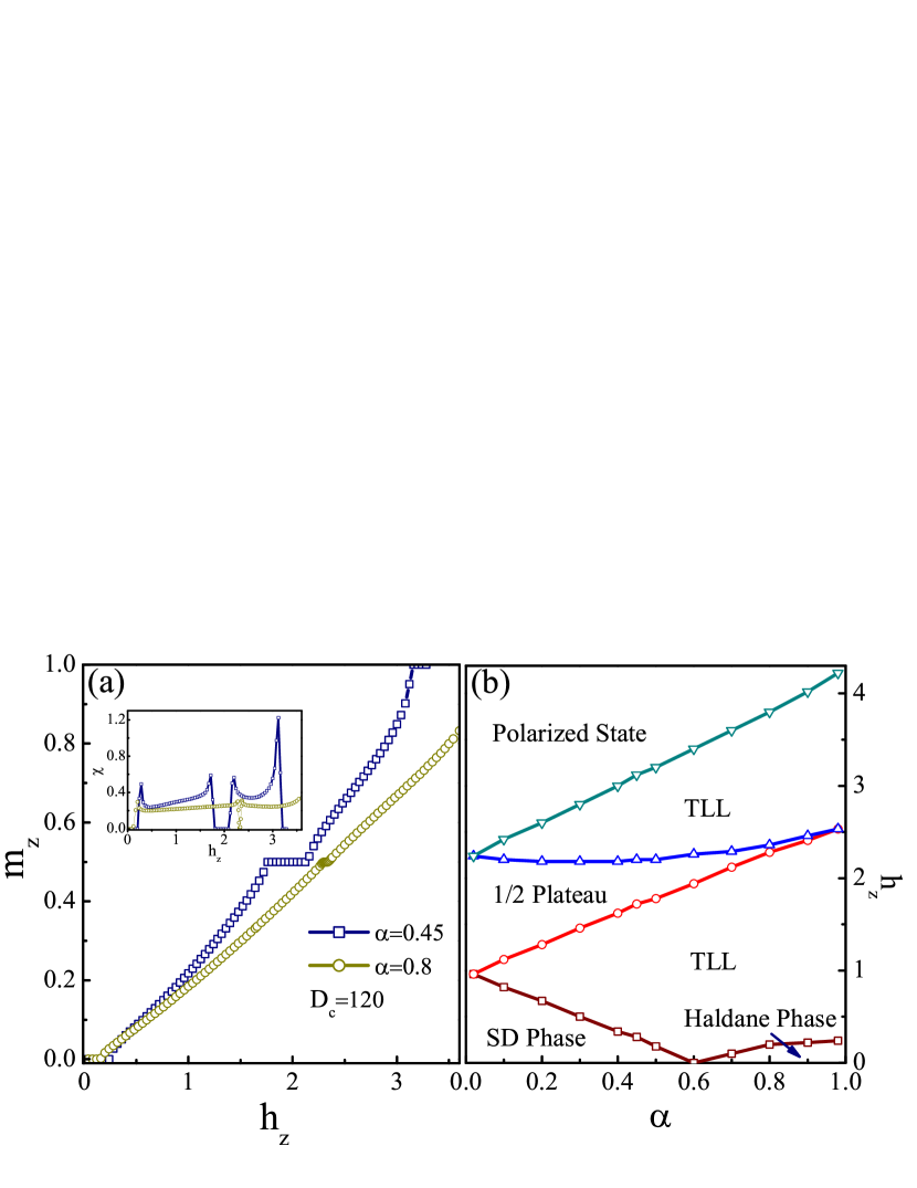
Figure 1: (Color online) (a) The magnetic curves of spin-1 bond alternating Heisenberg antiferromagnetic chain (BAHAFC) with a single-ion anisotropy in longitudinal magnetic fields $h_{z}$, where three magnetization plateaux ($m=0$, 1/2, and 1) are observed. The inset shows the singularities of the susceptibility as a function of magnetic field, which signal the occurrence of quantum phase transitions. (b) The ground state phase diagram in the plane of the bond alternating ratio ($\alpha$) vs. longitudinal magnetic field ($h_{z}$), where the Haldane, singlet-dimer (SD), m=1/2 magnetic plateau, Tomonaga-Luttinger liquid (TLL), and spin polarized phases are identified. The single-ion anisotropy $\Delta=0.25$ is taken.

Figure 1(a) presents the field dependence of magnetization per site $m_{z}$ for the system defined by Eq. (1) in the longitudinal magnetic field for $\alpha=0.45$ and $0.8$, where the bond dimension $D_{c}=120$ of a matrix product state is presumed. When $\alpha=0.45$, it is clear to see that there are three magnetization plateaux occurring at $m$=0, 1/2 and 1 in some regions of $h_{z}$. The $m$=0 plateau suggests that a gap remains in the absence of magnetic field, implying that the system is in the singlet-dimer phase, as it should be in the same phase as $\alpha=0$. Based on the valence-bond solid picture, the $m=1/2$ plateau corresponds to that one of the two bonds in each coupled spin-1 dimer is broken su . The $m=1$ plateau is in the spin fully polarized state. Near the critical fields, the magnetization per site $m_{z}$ depends on the magnetic field in a square root behavior, similar to the case of spin-1 HAFC in a magnetic field. In the ranges between the plateaus, the spin correlations should be in a power law decay, indicating a quasi long-range order. The critical magnetic fields for closure of the gap can be accurately determined by the field dependence of the susceptibility, where the sharp peaks appear, as shown in the inset of Fig. 1(a). When $\alpha=0.8$, the three magnetic plateaux still remain, but the width of $1/2$ plateau decreases, indicating that the corresponding gap becomes narrower. For the spin-1 BAHAFC, as the ground state period is $n=2$, the topological quantization condition $n(S-m)=integer$ is satisfied by $m$=0, 1/2 and 1, i.e., there should exist at most three plateaux in the longitudinal field for $0\leq\alpha<1$, which is well confirmed in Fig. 1(a). At the special case of $\alpha=1$, $n$ becomes 1, and there should be two plateaus at $m$=0 and 1.

For $0\leq\alpha\leq 1$, we have calculated the magnetization curves and the corresponding susceptibilities in the ground state, and collected all critical values of magnetic fields at which the susceptibility exhibits obvious singularities, which allows us for readily obtaining a global ground state phase diagram in $\alpha-h_{z}$ plane for the spin-1 BAHAFC with a single-ion anisotropy $\Delta=0.25$, as shown in Fig. 1(b). There are six phases, including the singlet-dimer (SD) phase, Haldane phase, two TLL phases separated by the $m=1/2$ magnetic plateau phase, and the spin fully polarized phase. At a critical bond alternating ratio $\alpha_{c}\approx 0.6$, there exists a quantum phase transition from the gapped SD state into the gapped Haldane phase. The $m$=1/2 plateau state persists for all values of $\alpha$ until it disappears at $\alpha=1$. At all six phase boundaries, the gap closes. In these phases, the spin-spin correlation function $\langle S_{i}^{z}S_{j}^{z}\rangle$ reveals different spatial behaviors, which is short-range ordered except that in the TLL phase it decays in an algebraic way.

II.3 Magnetization and Phase Diagram in a Transverse Field

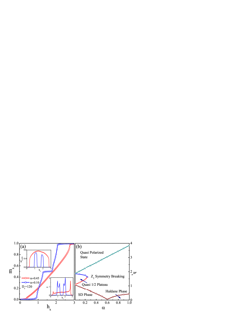
Figure 2: (Color online) (a) The magnetic curves of S=1 BAHAFC with a single-ion anisotropy in transverse magnetic fields $h_{x}$. The up-left inset shows the staggered magnetization along the $y$ axis, and the down-right inset presents the corresponding susceptibility as a function of magnetic field. For $\alpha=0.1$, three plateau-like steps are observed. (b) The ground state phase diagram in the plane of the bond alternating ratio ($\alpha$) vs. transverse magnetic field ($h_{x}$), where the Haldane, singlet-dimer (SD), Z₂ symmetry breaking Néel ordered, quasi 1/2 magnetic plateau, and quasi spin polarized phases are identified. The single-ion anisotropy $\Delta=0.25$ is taken.

In a transverse magnetic field $h_{x}$, the field dependence of magnetization per site $m_{x}$ and $m_{y}$ and the corresponding susceptibility of the model under interest are presented in Fig. 2(a) for $\alpha=0.1$ and 0.45. Three steps around $m_{x}$=0, 1/2 and 1 in magnetic curves ($m_{x}$ vs. $h_{x}$) are observed for $\alpha=0.1$. The corresponding susceptibility $\chi$ is illustrated in the lower inset of Fig. 2(a), where one may notice that, due to the non-conservation of total $S_{x}$, at these three steps $\chi$ does not exactly vanish although it is negligibly small. Thus, we call these steps as quasi magnetic plateaus. In the regions between the quasi plateaus, $m_{y}$ has large values as shown in the upper inset of Fig. 1(a). The reason is that the existence of the single-ion anisotropy makes the spins tend to arrange in $xy$ plane, and when the magnetic field is applied along the $x$ direction, the staggered magnetization $m_{y}$ is induced to form a canted Ising order. In addition, for $\alpha=0.1$ we observed from the upper inset of Fig. 2(a) that with increasing $h_{x}$ the staggered magnetization $m_{y}$ first is negligible small, and then exhibits a sharp valley structure, which illustrates a reentrant behavior of the staggered magnetization Diep ; Hieida . For $\alpha=0.45$, only two steps appear in the magnetic curve, and the quasi $m=1/2$ step disappears. In this case, $m_{y}$ has even larger values in the region between the two steps. For other larger $\alpha$, the magnetic curves in the transverse field $h_{x}$ have the behaviors similar to that of $\alpha=0.45$.

Utilizing the method similar to Fig. 1(b) and sweeping various values of $\alpha$, we can collect all critical magnetic fields by finding the singular positions of susceptibility, and then obtain the whole ground state phase diagram in $\alpha-h_{x}$ plane for the system under investigation, as depicted in Fig. 2(b). It can be seen that there are five phases, namely, the SD, Haldane, quasi $m=1/2$ magnetic plateau, Z₂ symmetry breaking (or spin canted) and the quasi spin polarized phases. The quantum critical point $\alpha_{c}\approx 0.6$ is recovered here. In contrast to the case under a longitudinal field where the $m=1/2$ plateau phase persists into the whole region of $\alpha<1$ and separates two TLL phases, the quasi $m=1/2$ plateau phase sets only in a small region ($\alpha\leq 0.24$). Starting from the SD and Haldane phases, when we increase the field $h_{x}$, the gap is gradually closed at the phase boundaries. If one continues to increase the magnetic field $h_{x}$, another gap opens because of the breaking of the discrete symmetry, giving rise to a Z₂ symmetry breaking phase, which displays a long range behavior.

III Entanglement Entropy and Conformal Anomalies

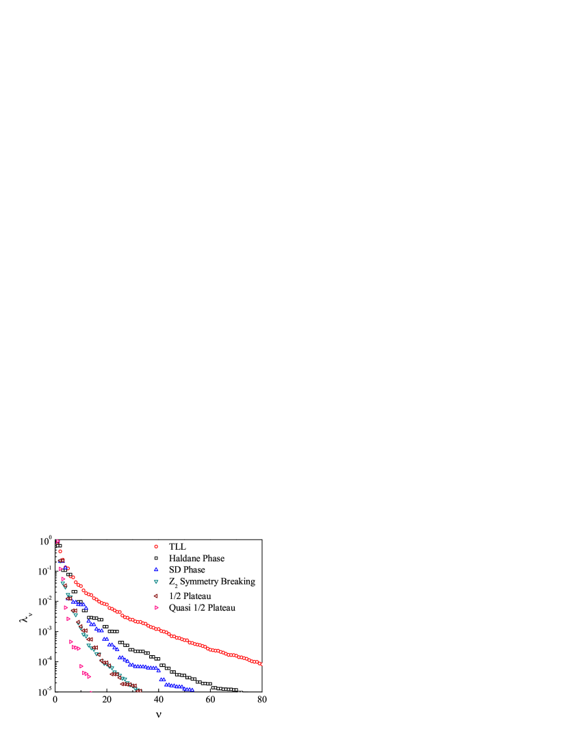
Figure 3: (Color online) The normalized Schmidt coefficient $\lambda_{\nu}$ as a function of the number of kept states $\nu$ for different phases, where $D_{c}=80$.

This present system demonstrates quite different behaviors in longitudinal and transverse magnetic fields. To gain further insight into the underlying physics behind this character, we have studied the conformal anomalies of this system at the critical regimes. The conformal field theory (CFT) tells us that the conformal invariance at the critical point sets useful constraints on the critical behaviors of two-dimensional classical or 1D quantum systems conformal , and the universality class can be characterized by the conformal anomaly or central charge $c$ of the Virasoro algebra. For a system with a continuous symmetry $G$, if G=SU(N), the possible conformal central charge is given by $c=(N^{2}-1)k/(N+k)$, $k=1,2,3,...$ Affleck0 . For the spin-S uniform antiferromagnetic quantum chains, G=SU(2), $c=3S/(1+S)$. For S=1/2, $c=1$; S=1, $c=3/2$. For the present spin-1 BAHAFC with a single-ion anisotropy, the SU(2) symmetry is not satisfied, and the conformal central charge should be calculated via other ways. The von Neumann entropy $S$, defined by

$$S=-Tr(\hat{\rho}_{sys}\log_{2}\hat{\rho}_{sys})=-Tr(\hat{\rho}_{env}\log_{2}\hat{\rho}_{env}),$$ (2)

offers a possible way to get the central charge of quantum spin chains, where $\hat{\rho}_{sys(env)}$ is the reduced density matrix (DM) of system (environment). In critical and noncritical regimes, the entanglement entropy has different asymptotic behaviors arealaw ; Vidal2 . In critical regimes, the CFT predicts wilczek

$$S\approx\frac{c}{3}\log_{2}(L)+k,$$ (3)

where $L$ is the number of spins for a block embedding in an infinite chain, $c$ is the central charge and $k$ is a non-universal constant. In noncritical regimes, $S$ vanishes for all L or grows monotonically with L until saturation. In the following, we shall invoke the iTEBD method to study the entanglement entropy for the case in a transverse magnetic field. Because of the nearly unitary evolution, the iTEBD algorithm gives the canonical form of infinite matrix product states (iMPS). We can make a Schmidt decomposition on the ground state wave function such that

$$|\psi\rangle=\sum_{\nu=1}^{D_{c}}\lambda_{\nu}|\psi^{A}_{\nu}\rangle|\psi^{B}_{\nu}\rangle$$ (4)

on each bond, where $|\psi_{\nu}^{A,B}\rangle$ is the orthonormalized basis states (Schmidt bases) for two parts $A$ and $B$ of the infinite chain, and $\lambda_{\nu}$ is the Schmidt coefficient (SC). Fig. 3 presents $\lambda_{\nu}$ as a function of $\nu$ for different phases. It is seen that in the TLL phase, the SC attenuates much slower than those in

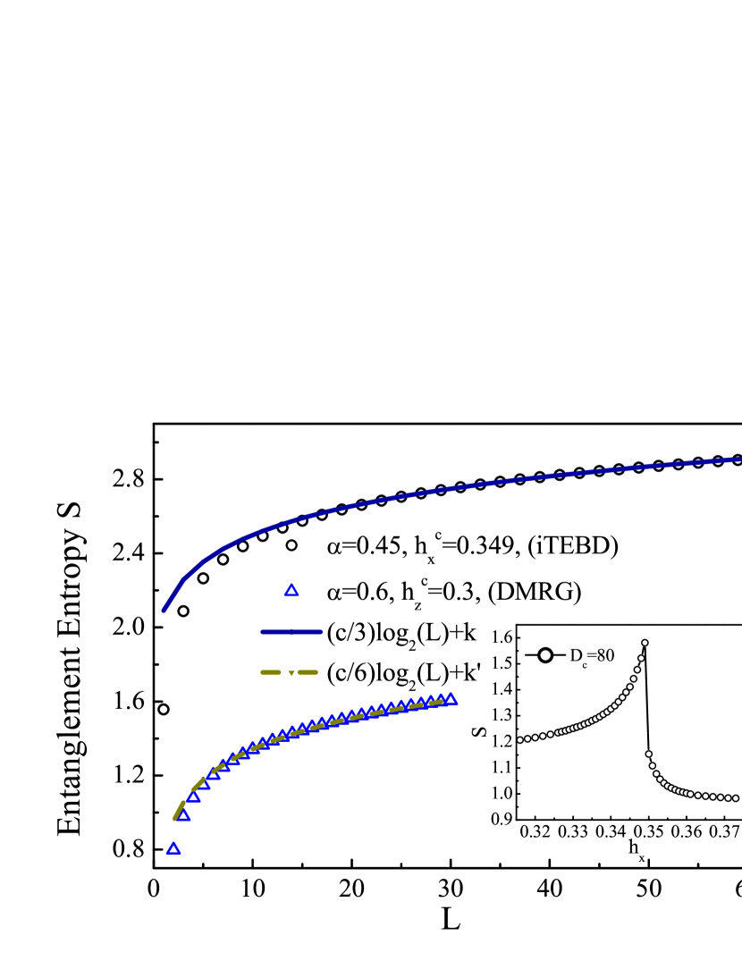
Figure 4: (Color online) The entanglement entropy $S$ as a function of chain length $L$ calculated by the iTEBD in a transverse field for $\alpha=0.45$ and $D_{c}=100$, and by the DMRG in a longitudinal magnetic field for $\alpha=0.6$ where the optimal states were kept as 400. In both cases, the single-ion anisotropy $\Delta=0.25$. The solid line is the fitting curve to Eq. (3), giving the central charge $c=1/2$ at a critical transverse field $h_{x}^{c}=0.349$; the inset shows that the entanglement entropy as a function of $h_{x}$ for a semi-infinite chain length is singular at $h_{x}^{c}=0.349$. The dashed line is the fitting curve for the case (TLL phase) at a longitudinal magnetic field $h_{z}=0.3$, giving the central charge $c=1$.

other gapped phases. The double degeneracy of SC only appears in the Haldane phase, indicating the existence of the topological string order entang_spectrum . Given a canonical form of iMPS, if the system in Eq. (2) is chosen as the semi-infinite chain, it is easy to directly calculate the von Neumann entropy, $S=-\sum_{\nu=1}^{D_{c}}\lambda_{\nu}^{2}\log_{2}(\lambda_{\nu}^{2})$. In addition, we can also calculate the entanglement entropy when the system is successive L spins embedding in an infinite chain, where we may set $L=2$ for an example. In particular, we can write

$$|\psi\rangle=\sum_{\alpha,\beta,\gamma=1}^{D_{c}}\sum_{i,j=1}^{d}\lambda_{\alpha}\Gamma^{i}_{\alpha,\beta}\lambda_{\beta}\Gamma^{j}_{\beta,\gamma}\lambda_{\gamma}|\Phi_{\alpha}\rangle|i\rangle|j\rangle|\Phi_{\gamma}\rangle,$$ (5)

where $\Gamma^{i}_{\alpha,\beta}$ is the tensor on the $i$-th site, $|i\rangle(|j\rangle)$ is the spin basis states on the $i(j)$-th site, $|\Phi_{\alpha}\rangle$ and $|\Phi_{\gamma}\rangle$ are the left Schmidt basis of the $i$-th site and the right Schmidt basis of the $j$-th site, respectively. By contracting two tensors, we will obtain the reduced DM

$$\hat{\rho} = Tr_{ij}|\psi\rangle\langle\psi|$$ (6)

$$= \sum_{\alpha,\gamma=1}^{D_{c}}\sum_{\alpha^{\prime},\gamma^{\prime}=1}^{D_{c}}[\sum_{i,j=1}^{d}\sum_{\beta,\beta^{\prime}=1}^{D_{c}}\lambda_{\alpha}\Gamma^{i}_{\alpha,\beta}\lambda_{\beta}\Gamma^{j}_{\beta,\gamma}\lambda_{\gamma}$$

$$\lambda_{\alpha^{\prime}}(\Gamma^{i}_{\alpha^{\prime},\beta^{\prime}})^{*}\lambda_{\beta^{\prime}}(\Gamma^{j}_{\beta^{\prime},\gamma^{\prime}})^{*}\lambda_{\gamma^{\prime}}]|\alpha\rangle|\gamma\rangle\langle\alpha^{\prime}|\langle\gamma^{\prime}|.$$

One can diagonalize this matrix and calculate the entanglement entropy. For a larger $L$, we need to contract $L$ tensors and select Schmidt basis to construct the reduced DM. For all $L$, the dimension of the reduced DM is $D_{c}^{2}\times{D_{c}^{2}}$. By calculating the von Neumann entropy for a semi-infinite chain in a transverse magnetic field, we observe that the cusp position of the entanglement entropy just gives the phase transition point $h_{x}^{c}=0.349(2)$. By fitting our calculated results to Eq. (3), we find $c=1/2$ for $h_{x}^{c}=0.349$, as shown in Fig. 4. In the TLL phase of the case in a longitudinal magnetic field, the iTEBD algorithm gives the ground state with a staggered magnetization perpendicular to $z$ direction so that it cannot yield a correct wave function. The reason is that there does not have an excitation gap and the iTEBD algorithm cannot project the right ground state wave function. In order to calculate the central charge in the TLL phase, we utilize the DMRG algorithm with open boundary condition at $h_{z}=0.3$, $\alpha=0.6$, and $\Delta=0.25$. The result is also included in Fig. 4, where the fitting result gives the central charge $c=1$ in this TLL phase note . Consequently, this implies that the critical behaviors of the spin-1 BAHAFC with a single-ion anisotropy in transverse fields quite differ from those in longitudinal fields, and the universality falls into two distinct classes with conformal central charges $c=1/2$ and $c=1$, respectively.

IV Thermodynamic Properties and Comparison to Experiments

IV.1 Susceptibility, Magnetization and Comparison to Experiments

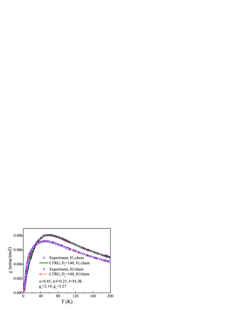
Figure 5: (Color online) The temperature dependence of susceptibility of NTENP measured experimentally is well fitted to the LTRG calculated data for both longitudinal and transverse magnetic fields. The experimental data are taken from Ref. [Narumi2, ].

The thermodynamic properties of this system were explored by using recently proposed LTRG algorithm Li that allows for accurately calculating the thermodynamic quantities at very low temperature. In the following LTRG calculations we keep the Trotter step $\tau=0.1$.

Fig. 5 gives the temperature dependence of susceptibilities of the spin-1 BAHAFC in longitudinal and transverse magnetic fields, where the fittings to the experimental data of NTENP under both fields are also included. One may see that the theoretical results are nicely fitted to the experimental data, generating a set of material parameters of NTENP: $\alpha=0.45$, $\Delta/J=0.25$, $J=54.2K$, $g_{\|}=2.14$, and $g_{\bot}=2.27$. It should be noted that in a longitudinal field, these parameters are in agreement with the previous results from the quantum Monte Carlo calculations Narumi2 , while in a transverse field the fitting to the experimental data of NTENP is for the first time done. The magnetization curves of NTENP were measured at T=1.3 K up to 700 kOe in Ref. [Narumi2, ], which are well fitted to our LTRG calculated results, giving the same set of fitting parameters as those obtained from the data of susceptibility except that $g_{\bot}=2.24$ here, as shown in Fig. 6. Considering that the two sets of experimental data from susceptibility and magnetic curves are independent, a slight difference on $g_{\bot}$ is reasonable. Thus, $g_{\bot}$ of NTENP should be around 2.24 $\sim$ 2.27. The high-field magnetization curve is also well fitted with our LTRG results (inset of Fig. (6)) using the same parameters.

Figure 6: (Color online) The magnetic curves of NTENP are well fitted to the LTRG calculated data for both longitudinal and transverse fields, where the fitting parameters are consistent with those from the susceptibilities. Inset is the high-field magnetic curve up to 700 kOe fitted with the corresponding LTRG calculated data. The experimental data are taken from Ref. [Narumi2, ].

IV.2 Specific Heat in Magnetic Fields

The temperature dependence of the specific heat $C(T)$ of the S=1 BAHAFC in longitudinal and transverse magnetic fields is obtained by the LTRG method down to very low temperatures, as shown in Fig. 7 for $h_{z}=0.5$ and $h_{x}=0.5$. In a transverse field, there are one round peak and a low temperature shoulder in $C(T)$, while in a longitudinal field the specific heat exhibits only one broad peak. It appears that at low temperature the specific heat displays distinct behaviors. To show this point clearly, we have carefully calculated the specific heat of this model at extremely low temperatures by the LTRG algorithm that is very powerful and efficient for calculating the low-temperature properties than other numerical methods gubo . Shown in the lower inset of Fig. 7, two different behaviors in both fields at low temperature are clearly demonstrated, where in a longitudinal field, the specific heat displays a linear T-dependent character, showing a TLL behavior, while in a transverse field, $C(T)$ exhibits an exponential decay (the fitting curve is given in the upper inset of Fig. 7), that can be ascribed to the $Z_{2}$ symmetry breaking with an open of an Ising gap.

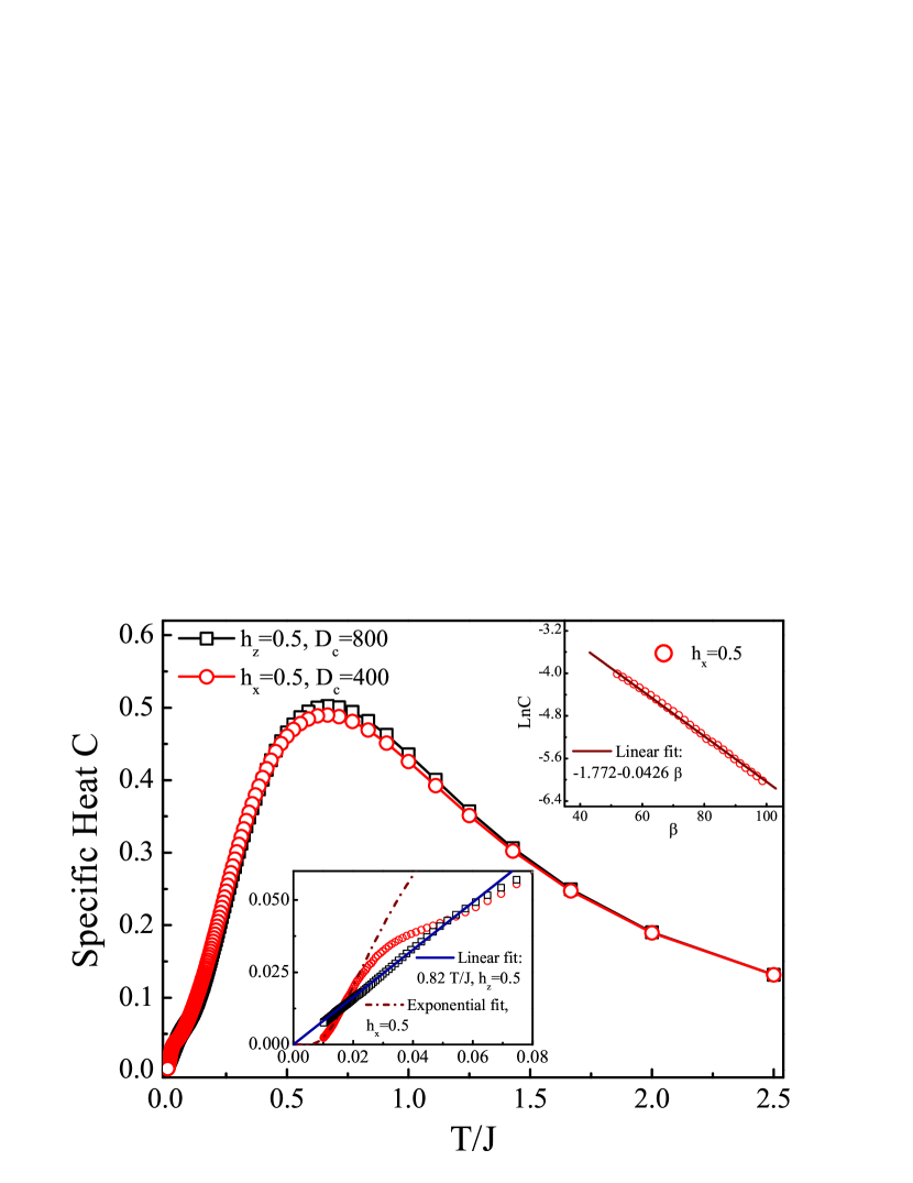
Figure 7: (Color online) The temperature dependence of the specific heat of S=1 BAHAFC under both longitudinal and transverse magnetic fields. Although the whole profiles look similar for both cases, the extremely low temperature behaviors shown in the down-left inset quite differ, where the linear-T dependence of the specific heat in a longitudinal field is clearly seen at low temperature, suggesting a Tomonaga-Luttinger liquid behavior, while an exponential decay for the T-dependence of the specific heat is observed in a transverse field owing to the appearance of an Ising gap, as seen in the up-right inset. The single-ion anisotropy $\Delta=0.25$ and the bond alternating ratio $\alpha=0.45$ are taken.

The specific heat $C(T)$ of NTENP was also measured experimentally Hagiwara2 , where the linear T-dependence of $C(T)$ at low temperature in a longitudinal field above the critical field $h{{}_{z}}^{c}=9.3$ T was observed, which was identified as a TLL behavior. Our low temperature LTRG calculations at $h_{z}=0.5$ ($>h{{}_{z}}^{c}$) on the S=1 BAHAFC model strongly supports this experimental observation. In a transverse field, the experiment on NTENP gives a distinct nonlinear low-temperature behavior of $C(T)$ from that in a longitudinal field, which is also backed up by our LTRG results. We should remark here that the sharp peaks in the temperature dependent specific heat of NTENP were observed in both fields, which cannot be explained by using this spin-1 BAHAFC model, as revealed by our present studies, because we do not find any field-dependent sharp peaks of $C(T)$ in this 1D model. Those sharp peaks may signal the field-induced long-range orders from the 3D effect of inter-chain interactions in NTENP. It is this reason that makes us not directly fit our LTRG results with the experimental data of specific heat of NTENP. Nevertheless, our present studies on the spin-1 BAHAFC model may give a possible clue to understand the experimentally observed low-temperature sharp peaks of $C(T)$ Hagiwara2 . In a longitudinal field, as long as the magnetic field is higher than the critical field ($h{{}_{z}}^{c}$), the system will enter the TLL phase that has a quasi LRO, and the true LRO can be established only by interchain couplings. Thus the peak position is almost determined by the strength of interchain interactions and hardly moves with the increase of the magnetic field. In a transverse field, in the range that the experiment was performed, the staggered magnetization that could enhance the interchain couplings increases monotonously with increasing the magnetic field, so the low-temperature sharp peak moves to the high temperature side with the increase of the transverse field.

V Summary and Conclusion

In summary, we have investigated the spin-1 BAHAFC model with a single-ion anisotropy in longitudinal and transverse magnetic fields by employing the iTEBD and LTRG methods. The ground state phase diagrams in the plane of field versus the bond alternating ratio under both fields are obtained, where various phases are identified for two cases. From the entanglement entropy, the conformal central charges in both critical longitudinal and transverse fields are determined to be $c=1$ and $1/2$, respectively, suggesting that the universality in critical regimes falls into different classes for both fields. The TLL behavior at low $T$ observed experimentally in NTENP is verified via our accurate calculations, while an exponential decay of low-temperature specific heat is uncovered in a transverse field. The experimental data of the model material NTENP are well fitted with our LTRG results, and the parameters for characterizing NTENP are determined.

- (1) † These authors contribute equally to this work.
- (2) A. S. Darmawan, and S. D. Bartlett, Phys. Rev. A 82, 012328 (2010).
- (3) S. Ma, C. Broholm, D. H. Reich, B. J. Sternlieb, and R. W. Erwin, Phys. Rev. Lett. 69, 3571 (1992)
- (4) Y. Narumi, M. Hagiwara, R. Sato, K. Kindo, H. Nakano, and M. Takahashi, Physica B 509, 246-247 (1998).
- (5) Y. Narumi, K. Kindo, M. Hagiwara, H. Nakano, A. Kawaguchi, K. Okunishi, M. Kohno, Phys. Rev. B 69, 174405 (2004).
- (6) A. Escuer, R. Vicente, and X. Solans, J. Chem. Soc. Dalton Trans. (1997), 531.
- (7) Y. Narumi, M. Hagiwara, M. Kohno, and K. Kindo, Phys. Rev. Lett. 86, 324 (2001).
- (8) A. Zheludev, T. Masuda, B. Sales, D. Mandrus, T. Papenbrock, T. Barnes, and S. Park, Phys. Rev. B 69, 144417 (2004).
- (9) M. Hagiwara, L. P. Regnault, A. Zheludev, A. Stunault, N. Metoki, T. Suzuki, S. Suga, K. Kakurai, Y. Koike, P. Vorderwisch, and J. -H. Chung, Phys. Rev. Lett. 94, 177202 (2005).
- (10) T. Suzuki and S. Suga, Phys. Rev. B 72, 014434 (2005).
- (11) L. P. Regnault, A. Zheludev, M. Hagiwara, and A. Stunault, Phys. Rev. B 73, 174431 (2006).
- (12) M. Hagiwara, H. Tsujii, C.R. Rotundu, B. Andraka, Y. Takano, N. Tateiwa, T.C. Kobayashi, T. Suzuki, and S. Suga, Phys. Rev. Lett. 96, 147203 (2006).
- (13) V. N. Glazkov, A. I. Smirnov, A. Zheludev and B. C Sales, Phys. Rev. B 82, 184406 (2010).
- (14) M. Oshikawa, M. Yamanaka, and I. Affleck, Phys. Rev. Lett. 78, 1984 (1997).
- (15) B. Gu, G. Su, and S. Gao, J. Phys.: Condens. Matter 17, 6081 (2005); B. Gu, G. Su, and S. Gao, Phys. Rev. B 73, 134427 (2006); B. Gu and G. Su, Phys. Rev. Lett. 97, 089701 (2006); Phys. Rev. B 75, 174437 (2007); S. S. Gong and G. Su, ibid. 78, 104416 (2008); S. S. Gong, S. Gao, and G. Su, ibid. 80, 014413 (2009); S. S. Gong and G. Su, Phys. Rev. A 80, 012323 (2009); Y. Zhao, S. S. Gong, W. Li, and G. Su, Appl. Phys. Lett. 96, 162503 (2010); S. S. Gong, W. Li, Y. Zhao, and G. Su, Phys. Rev. B 81, 214431 (2010).
- (16) G. Gómez-Santos, Phys. Rev. Lett. 63, 790 (1989).
- (17) A. M. Tsvelik, Phys. Rev. B 42, 10499 (1990).
- (18) R. R. P. Singh and M. P. Gelfand, Phys. Rev. Lett. 61, 2133 (1988).
- (19) M. Kohno and M. Takahashi, Phys. Rev. B 57, 1046 (1998).
- (20) A. Kitazawa, K. Nomura, and K. Okamoto, Phys. Rev. Lett. 76, 4038 (1996).
- (21) I. Affleck, Phys. Rev. B 43, 3215 (1991).
- (22) Z. C. Gu and X. G. Wen, Phys. Rev. B 80, 155131 (2009).
- (23) H. Z. Xing, G. Su, S. Gao, and J. H. Chu, Phys. Rev. B 66, 054419 (2002).
- (24) G. Vidal, Phys. Rev. Lett. 98, 070201 (2007); R. Orús and G. Vidal, Phys. Rev. B 78, 155117 (2008).
- (25) W. Li, S.-J. Ran, S.-S. Gong, Y. Zhao, B. Xi, F. Ye, and G. Su, Phys. Rev. Lett. 106, 127202 (2011).
- (26) S. R. White, Phys, Rev. Lett. 96, 2863 (1992).
- (27) P. Azaria, H. T. Diep, and H. Giacomini, Phys. Rev. Lett. 59, 1629 (1987).
- (28) Y. Hieida, K. Okunishi, and Y. Akutsu, Phys. Rev. B 64, 224422 (2001).
- (29) A. A. Belavin, A. M. Polyakov, and A. B. Zamolodchikov, J. Stat. Phys. 34, 763 (1984); Nucl. Phys. B 241, 333 (1984); D. Friedan, Z, Qiu, and S. Shenker, Phys. Rev. Lett. 52, 1575 (1984).
- (30) I. Affleck, Phys. Rev. Lett. 56, 746 (1986).
- (31) H. W. G. Blöte, J. L. Cardy, and M. P. Nightingale, Phys. Rev. Lett. 56, 742(1986).
- (32) G. Vidal, J. I. Latorre, E. Rico, and A. Kitaev, Phys. Rev. Lett. 90, 227902 (2003).
- (33) J. Eisert, M. Cramer, and M. B.Plenil, Rev. Mod. Phys. 82, 277 (2010).
- (34) C. Holzhey, F. Larsen, and F. Wilczek, Nucl. Phys. B 424, 443 (1994).
- (35) F. Pollmann, A. M. Turner, E. Berg, M. Oshikawa, Phys. Rev. B 81, 064439 (2010).
- (36) In the infinite chain DMRG algorithm with open boundary condition, the entanglement entropy in critical regimes should take the form of ; see also P. Calabrese, and J. Cardy, J. Stat. Mech. P06002 (2004).
- (37) B. Gu, Ph. D. Thesis, Graduate University of Chinese Academy of Sciences, Beijing, China, (2006).