Differential rotation of main-sequence dwarfs: predicting the dependence on surface temperature and rotation rate

Abstract

Gyrochronology and recent theoretical findings are used to reduce the number of input parameters of differential rotation models. This eventually leads, after having fixed our turbulence model parameters, to a theoretical prediction for the surface differential rotation as a function of only two stellar parameters - surface temperature and rotation period - that can be defined observationally. An analytical approximation for this function is suggested. The tendency for the differential rotation to increase with temperature is confirmed. The increase is much steeper for late F-stars compared to G- and K-dwarfs. Slow and fast rotation regimes for internal stellar rotation are identified. A star attains its maximum differential rotation at rotation rates intermediate between these two regimes. The amplitude of the meridional flow increases with surface temperature and rotation rate. The structure of the flow changes considerably between cases of slow and fast rotation. The flow in rapid rotators is concentrated in the boundary layers near the top and bottom of the convection zone with very weak circulation in between.

1 Introduction

Rotation of the sun and other stars with external convection zones is not uniform. The rotation period depends on latitude and typically increases from the equator to the poles (Donahue et al., 1996; Collier Cameron, 2003, 2007). The phenomenon of differential rotation is closely related to magnetic activity and has long been a subject of theoretical studies. The currently leading theoretical concept pioneered by Lebedinskii (1941) explains differential rotation by the interaction between convection and rotation. Convective motions in a rotating star are disturbed by Coriolis force. Back reaction disturbs rotation to make it not uniform.

Theoretical models reproduce the observed rotation of the sun quite closely (Kitchatinov & Rüdiger, 2005; Miesch et al., 2006). In the case of the sun, however, the differential rotation theory has to explain what is already known from helioseismology. The detailed helioseismological picture of the internal solar rotation (Wilson et al., 1997; Schou et al., 1998) left no opportunity for theoretical predictions. The theory then has to test its predictive ability with other stars, and this is very tempting to do in view of the rapid development of asteroseismology (Christensen-Dalsgaard & Houdek, 2010). Some computations of differential rotation as a function of stellar mass and rotation rate have been already attempted (Kitchatinov & Rüdiger, 1999) and were even to some extent supported by observations (Barnes et al., 2005). A systematic study of stellar differential rotation was, however, not possible because the stellar parameters on which it depends are too many. The resulting differential rotation depends on mass, chemical composition (metallicity), rotation period, and age of a star. Exploring four-dimensional parametric space is an unbearable task.

The situation has changed recently. First, the development of a new branch of astronomy named Gyrochronology has led to the establishment of a functional relation between stellar mass, age, and rate of rotation (Barnes, 2003, 2007, 2010; Collier Cameron et al., 2009; Meibom et al., 2009). Second, theoretical modeling shows that main-sequence stars of different mass and metallicity have (almost) the same differential rotation when their surface temperatures coincide (Kitchatinov & Olemskoy 2011, hereafter KO11). In other words, the dependencies on mass and metallicity can be combined into a common dependence on effective temperature. These two developments reduce the number of independent parameters on which differential rotation depends by two. The dependence on the remaining two parameters can well be explored numerically.

In our preceding publication (KO11), a new mean-field model for differential rotation was presented. Performance of the model was tested by applying it to the sun and individual stars including two rapid rotators (AB Dor and LQ Hya) and two moderate rotators ($\epsilon$ Eri and $\kappa^{1}$ Ceti) whose rotation has been studied well observationally (Donati & Collier Cameron, 1997; Kovári et al., 2004; Croll et al., 2006; Walker et al., 2007). The temperature dependence of differential rotation of young stars observed by Barnes et al. (2005) was modeled. This new paper reports and summarizes the results of extensive computations of stellar differential rotation. We find that after a solar-like star arrives at the main sequence, its differential rotation initially increases and then decreases as the star ages. The rotation period, at which the differential rotation is maximum, decreases with stellar mass. The dependence on rotation rate is, however, mild. The differential rotation depends more strongly on surface temperature, the hotter the star, the larger it is. In this paper, we suggest an analytical approximation for the numerically defined dependence of differential rotation on rotation period and surface temperature. The theoretical prediction can be tested by observations if only rotation period, surface temperature and the surface differential rotation are simultaneously measured. Dependence of the meridional flow amplitude and structure on rotation rate and temperature is also studied. The next Section 2 describes our model and method. Section 3 presents and discusses the results, which are summarized in Section 4.

2 Model and method

2.1 The model

Our model is based on the mean-field theory of differential rotation. This means that the velocity field ($v$) is split in its mean ($V$) and fluctuating ($u$) parts,

$${\mbox{\boldmath$v$}}={\mbox{\boldmath$V$}}+{\mbox{\boldmath$u$}},\ \ \ {\mbox{\boldmath$V$}}=\langle{\mbox{\boldmath$v$}}\rangle,\ \ \ \langle{\mbox{\boldmath$u$}}\rangle=0,$$ (1)

and equations for the mean flow, $V$, are formulated. The equations are then solved numerically. The angular brackets in (1) signify an averaging procedure that smoothes out random fluctuations of turbulent fields. The steady equation for the mean flow,

$$\left({\mbox{\boldmath$V$}}\cdot{\mbox{\boldmath$\nabla$}}\right){\mbox{\boldmath$V$}}+\frac{1}{\rho}{\mbox{\boldmath$\nabla$}}P-{\mbox{\boldmath$g$}}=\frac{1}{\rho}{\mbox{\boldmath$\nabla$}}\cdot{\mbox{\boldmath$R$}},$$ (2)

involves the effects of turbulence via the Reynolds stress tensor,

$$R_{ij}=-\rho\langle u_{i}u_{j}\rangle.$$ (3)

In equation (2), $\rho$, $P$, and $g$ are the mean density, pressure, and gravity respectively. Reynolds stress (3) includes two parts representing the turbulent viscosity and non-viscous flux of momentum,

$$R_{ij}=-\rho Q^{\Lambda}_{ij}+\rho{\cal N}_{ijkl}\frac{\partial V_{k}}{\partial r_{l}},$$ (4)

where the summation convention over the repeated subscripts is assumed, ${\cal N}_{ijkl}$ is the eddy viscosity tensor, and $Q^{\Lambda}_{ij}$ represents the non-viscous part of the stress (cf. Appendix of KO11 for detailed expressions for both parts of the Reynolds stress (4)). The presence of non-viscous flux of angular momentum in rotating turbulent fluids was called the ‘$\Lambda$-effect’ (Rüdiger, 1989). This effect is the principal driver of differential rotation in our model.

The direction of the angular momentum transport by the $\Lambda$-effect is controlled by two dimensionless parameters, $V^{(0)}$ and $H^{(1)}$, of the $Q^{\Lambda}$-tensor

$$Q_{ij}^{\Lambda} = \nu_{{}_{\mathrm{T}}}\Omega_{k}\hat{r}_{l}\left(V^{(0)}(\Omega^{*})\left(\hat{r}_{i}\varepsilon_{jkl}+\hat{r}_{j}\varepsilon_{ikl}\right)\right.$$ (5)

$$+ \left.H^{(1)}(\Omega^{*})\frac{\left({\hat{\mbox{\boldmath$r$}}}\cdot{\mbox{\boldmath$\Omega$}}\right)}{\Omega^{2}}\left(\Omega_{i}\varepsilon_{jkl}+\Omega_{j}\varepsilon_{ikl}\right)\right),$$

where $\Omega$ is the angular velocity vector, $\hat{\mbox{\boldmath$r$}}$ is the radial unit vector,

$$\nu_{{}_{\mathrm{T}}}=-\frac{\tau\ell^{2}g}{15c_{\mathrm{p}}}\frac{\partial S}{\partial r}$$ (6)

is the eddy viscosity parameter, $S$ is the specific entropy, $g$ is gravity, $c_{\mathrm{p}}$ is the specific heat at constant pressure, $\ell=\alpha_{{}_{\mathrm{MLT}}}H_{\mathrm{p}}$ is the mixing length, $H_{\mathrm{p}}$ is the pressure scale height,

$$\Omega^{*}=2\tau\Omega$$ (7)

is the Coriolis number,

$$\tau=\left(\frac{4c_{\mathrm{p}}\rho\ell^{2}T}{3g\delta F}\right)^{1/3}$$ (8)

is the convective turnover time, $\delta F=L(4\pi r^{2})^{-1}-F^{\mathrm{rad}}$ is the ‘residual’ heat flux that convection has to transport, and $F^{\mathrm{rad}}$ is the radiative heat flux.

Coriolis number (7) measures the intensity of interaction between convection and rotation. Its value defines whether the turbulent eddies are living long enough for rotation to influence them considerably. The Coriolis number, $\Omega^{*}=4\pi\mathrm{Ro}^{-1}$, is reciprocal to the Rossby number $\mathrm{Ro}=P_{\mathrm{rot}}\tau^{-1}$; $P_{\mathrm{rot}}$ is the rotation period. Explicit expressions for the functions $V^{(0)}(\Omega^{*})$ and $H^{(1)}(\Omega^{*})$ of (5) were derived by Kitchatinov & Rüdiger (1995,2005). In the slow rotation limit, $\Omega^{*}\ll 1$, $H^{(1)}(\Omega^{*})$ is small compared to $V^{(0)}(\Omega^{*})$ and $V^{(0)}(\Omega^{*})$ is negative. This means that the non-diffusive flux of angular momentum is close to the inward radial direction. In the opposite limit of rapid rotation, $\Omega^{*}\gg 1$, $V^{(0)}(\Omega^{*})$ is small compared to $H^{(1)}(\Omega^{*})$. Angular momentum flux is parallel to the rotation axis and points to the equatorial plane in this case. As the Coriolis number increases from small to large values, the angular momentum transport by the $\Lambda$-effect changes smoothly from radial inward to equatorward and parallel to the rotation axis. This picture generally agrees with 3D numerical simulations of Käpylä & Brandenburg (2008) and Käpylä et al. (2011).

The differential rotation model of this paper is identical to that of KO11. A detailed formulation of the model can be found in that paper and in the references given there. We just outline the model here.

The azimuthal component of Eq. (2) in spherical coordinates ($r,\theta,\phi$) gives the mean-field equation for the angular momentum balance,

$$\mathrm{div}\left(\rho r\sin\theta\langle u_{\phi}\mbox{\boldmath$u$}\rangle+\rho r^{2}\sin^{2}\theta\ \Omega\mbox{\boldmath$V$}^{\mathrm{m}}\right)=0,$$ (9)

where ${\mbox{\boldmath$V$}}^{\mathrm{m}}$ is the meridional flow velocity. Upon substitution of an explicit expression for Reynolds stress in (9), an equation for angular velocity can be obtained, which involves the meridional flow and is thus not closed.

The origin of meridional flow can be seen from the equation, which can be obtained as the azimuthal component of the curled equation (2),

$${\cal D}(\mbox{\boldmath$V$}^{\mathrm{m}})\ =\ \sin\theta\ r{\partial\Omega^{2}\over\partial z}\ -\ {g\over c_{\rm p}r}{\partial S\over\partial\theta},$$ (10)

where $\partial/\partial z=\cos\theta\partial/\partial r-r^{-1}\sin\theta\partial/\partial\theta$ is the spatial derivative along the rotation axis. The left part of this equation describes the viscous drag on the meridional flow

$${\cal D}(\mbox{\boldmath$V$}^{\mathrm{m}})\ \equiv-\varepsilon_{\phi jk}\frac{\partial}{\partial r_{j}}\left(\frac{1}{\rho}\frac{\partial}{\partial r_{l}}\left(\rho\ {\cal N}_{klmn}\frac{\partial V_{m}}{\partial r_{n}}\right)\right)$$ (11)

(see Appendix in KO11 for the expression for ${\cal D}(\mbox{\boldmath$V$}^{\mathrm{m}})$ in spherical coordinates).

The right part of the meridional flow equation (10) includes two sources of meridional flow: the centrifugal driving of the flow by non-conservative part of centrifugal force (known also as the ‘gyroscopic pumping’) and the baroclinic driver due to the meridional gradient of entropy (thermal wind). Each term on the right side of (10) is large compared to the left side. The two terms on the right, therefore, almost balance each other, this state is known as the Taylor-Proudman balance. The meridional flow results from a slight deviation from the balance. The meridional flow attains its largest velocities near the boundaries of the convection zone because the stress-free boundary conditions are not compatible with the Taylor-Proudman balance. Therefore, the Taylor-Proudman balance has to be violated near the stress-free boundaries where the source of meridional flow in the right side of (10) attains its largest values (Kitchatinov & Rüdiger, 1999; Miesch & Hindman, 2011).

Direction of the convective heat flux,

$$F^{\mathrm{conv}}_{i}=-\rho T\chi_{ij}\frac{\partial S}{\partial r_{j}},$$ (12)

depends on the structure of the eddy conductivity tensor,

$$\chi_{ij}=\chi\delta_{ij}+\chi_{\|}\frac{\Omega_{i}\Omega_{j}}{\Omega^{2}}.$$ (13)

The rotationally induced anisotropy of the conductivity (13) results in a deviation of the heat flux (12) from a radial direction to the poles, which in turn produces the dependence of entropy on latitude. This ‘differential temperature’ is, therefore, produced not only by the dependence of thermal conductivity on latitude (Weiss, 1965) but mainly by the anisotropy of the conductivity (Rüdiger et al., 2005).

The model solves the system of three joint equations governing distributions of angular velocity, meridional flow, and entropy inside the convection zone. These steady equations are solved numerically by the relaxation method.

It should be noted that the model relies on a uniform theoretical basis: all the model needs, including the $\Lambda$-effect, eddy viscosities and thermal conductivities was derived within the same quasi-linear approximation of turbulence theory. In particular, the eddy conductivities (13) were derived as fully nonlinear functions of the Coriolis number:

$$\chi=\chi_{{}_{\mathrm{T}}}\phi(\Omega^{*}),\ \ \ \chi_{\|}=c_{\chi}\chi_{{}_{\mathrm{T}}}\phi_{\|}(\Omega^{*})$$ (14)

(Kitchatinov et al., 1994). In this equation, $\chi_{{}_{\mathrm{T}}}$ is the isotropic eddy conductivity which would take place under actual sources of turbulence (actual superadiabaticity) but in non-rotating fluid. The mixing-length relation

$$\chi_{{}_{\mathrm{T}}}=-\frac{\tau\ell^{2}g}{12c_{\mathrm{p}}}\frac{\partial S}{\partial r},$$ (15)

defines the conductivity in terms of the entropy gradient. This gradient is controlled by the solution of the model equations. Similarly, the eddy viscosity tensor,

$${\cal N}_{ijkl} = \nu_{1}\left(\delta_{ik}\delta_{jl}\ +\ \delta_{jk}\delta_{il}\right)$$ (16)

$$+ \nu_{2}\big{(}\delta_{il}\frac{\Omega_{j}\Omega_{k}}{\Omega^{2}}+\delta_{jl}\frac{\Omega_{i}\hat{\Omega}_{k}}{\Omega^{2}}$$

$$+ \delta_{ik}\frac{\Omega_{j}\hat{\Omega}_{l}}{\Omega^{2}}+\delta_{jk}\frac{\Omega_{i}\hat{\Omega}_{l}}{\Omega^{2}}+\delta_{kl}\frac{\Omega_{i}\hat{\Omega}_{j}}{\Omega^{2}}\big{)}$$

$$+ \nu_{3}\delta_{ij}\delta_{kl}-\nu_{4}\delta_{ij}\frac{\Omega_{k}\hat{\Omega}_{l}}{\Omega^{2}}+\nu_{5}\frac{\Omega_{i}\hat{\Omega}_{j}\hat{\Omega}_{k}\hat{\Omega}_{l}}{\Omega^{4}},$$

involves the rotationally induced anisotropy and quenching via dependence of the viscosity coefficients

$$\nu_{n}=\nu_{{}_{\mathrm{T}}}\phi_{n}(\Omega^{*})\ \ \ \ n=1,2,...5$$ (17)

on the Coriolis number (7). Explicit expressions for the viscosity quenching functions, $\phi_{n}(\Omega^{*})$, are given in Kitchatinov et al. (1994) and the background viscosity $\nu_{{}_{\mathrm{T}}}$ is defined in terms of the entropy gradient in (6).

In other words, all the eddy transport coefficients are not prescribed but computed. Such an approach helps to avoid arbitrariness in prescribing uncertain parameters. Still, two parameters remained for some time uncertain. First, the $\Lambda$-effect depends - apart from the well known (nearly adiabatic) density stratification - also on turbulence anisotropy, which is uncertain. The contribution of anisotropy was put to zero in the former version of our model (Kitchatinov & Rüdiger, 1999) but then fixed by comparison with 3D f-plane simulations of thermal convection (Kitchatinov & Rüdiger, 2005) and never varied since then. Second, the $c_{\chi}$ parameter of (14) is uncertain ($c_{\chi}=1$ in Kitchatinov & Rüdiger 1999). It was found in KO11 that $c_{\chi}=1.5$ gives close agreement with helioseismology. Since then, $c_{\chi}=1.5$ is used for stellar applications also (Küker et al., 2011) and not varied any more. It is $c_{\chi}=1.5$ in this paper also.

After the two uncertain parameters were fixed, no further tuning is possible in the mean-field model for differential rotation. In this sense, the model does not have free parameters.

2.2 Reducing the number of input parameters

Input parameters of the model include the rotation period ($P_{\mathrm{rot}}$) and a set of parameters, all of which can be taken from a structure model of a (non-rotating) star. We use the EZ code of stellar evolution by Paxton (2004) to specify the structure of a main-sequence star of given mass, age, and metallicity. The four basic input parameters - rotation period, mass, age, and metallicity - are, however, not independent.

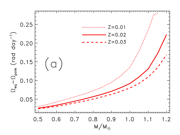
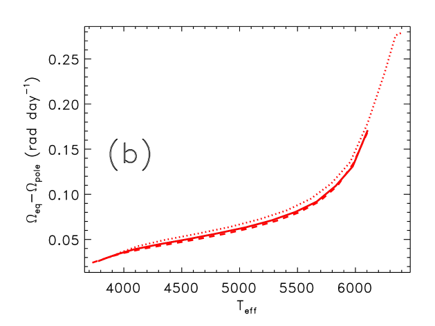
Figure 1: Surface differential rotation as function of stellar mass (a) and surface temperature (b) after our model. Lines of different styles correspond to different metallicities $Z$. Computations were performed for 1 Gyr old stars with $P_{\mathrm{rot}}=10$ days.

Figure 1 shows the surface differential rotation computed with our model for stars of different mass and metallicity. All stars are at the age of 1 Gyr. A rotation period $P_{\mathrm{rot}}=10$ days was prescribed. The dependence on metallicity for stars of given mass is quite pronounced. However, the dependence almost disappears when differential rotation is considered as a function of surface temperature. The same scaling was found in KO11 for ZAMS stars with $P_{\mathrm{rot}}=1$ day. We conclude that the values of surface differential rotation computed for stars of different masses and metallicities but fixed rotation period lie on a single line when plotted as a function of the effective temperature ($T_{\mathrm{eff}}$). A number of other computations were done to confirm this temperature-scaling for stars with not too low metallicities (Population I stars). The scaling reduces the number of input parameters by one: the mass and metallicity dependencies are combined into a common dependence on temperature.

Further reduction is achieved by using Gyrochronology. The rotation rate of solar- and late-type stars is a function of $T_{\mathrm{eff}}$ and age ($t$). Gyrochronology generalizes the Skumanich (1972) law, $P_{\mathrm{rot}}\propto t^{0.5}$, by specifying the proportionality constant in this law as a function of $T_{\mathrm{eff}}$ or other equivalent parameter. We use the empirical relation of Barnes (2007),

$$P_{\mathrm{rot}}=at^{n}\left(B-V-c\right)^{b}\ \mathrm{days},$$ (18)

with $n=0.519$, $a=0.773$, $b=0.601$, $c=0.4$, to specify the rotation period of a star of given $B-V$ colour and age $t$ measured in Myr. The relation does not apply to very young rapidly rotating stars of the so-called ‘C-sequence’ (Barnes, 2007). The structure of a star, however, changes little over its C-sequence life. Therefore, the relation (18) can still be used for our purposes even for very young stars. We used the tables of colour-temperature relations and the interpolation code of VandenBerg & Clem (2003) to compute $B-V$ colour of Eq. (18).

In this paper we fix the metallicity $Z=0.02$ and compute differential rotation for main-sequence dwarfs of different masses and ages. The computations cover the mass range from $0.5M_{\odot}$ to $1.3M_{\odot}$. The stellar masses were spanned by $0.05M_{\odot}$ in the range of $0.5\leq M/M_{\odot}\leq 1.1$. The mass dependence of differential rotation steepens for more massive stars. Accordingly, the span was reduced to $0.025M_{\odot}$ for the range of $1.1\leq M/M_{\odot}\leq 1.3$. For a given mass, structure models were generated for a sequence of ages. Then, rotation periods of Eq. (18) were estimated for every age and corresponding structure, and a sequence of differential rotation models was computed. This gives the differential rotation as a table-given function of rotation period and temperature. The surface differential rotation is then approximated by a neural network with one hidden layer (Conway, 1998):

$$\Delta\Omega=W_{0}+\sum\limits_{n=1}^{N}W_{n}\tanh\left(w_{n}+w^{T}_{n}T_{\mathrm{eff}}+w^{P}_{n}P_{\mathrm{rot}}\right),$$ (19)

where $\Delta\Omega=\Omega_{\mathrm{eq}}-\Omega_{\mathrm{pole}}$ is the angular velocity difference between the equator and pole. The convenience of this approximation is related to i) its universality: any continuous function can be represented by one hidden layer network to an arbitrary accuracy given sufficiently large $N$, and ii) availability of reliable numerical routines for tuning the parameters of the network (19). Using the regression formula (19), a theoretical prediction for the surface differential rotation of a star can be inferred from an observed rotation period and effective temperature.

3 Results and discussion

Figures 2 and 3 show the computed differential rotation as a function of the rotation period for a variety of stellar masses. Lines of these plots were computed for a certain initial mass but not for a given stellar structure. The structure changes as a star ages and rotation period increases.

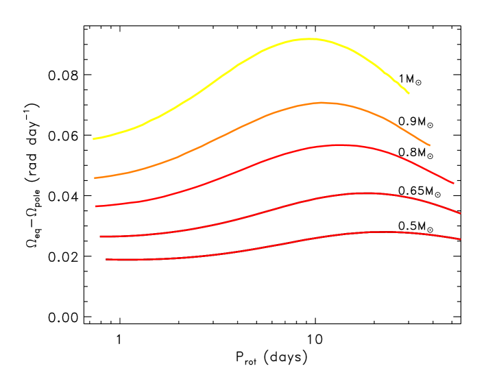
Figure 2: Surface differential rotation as a function of the rotation period for stars of subsolar masses.

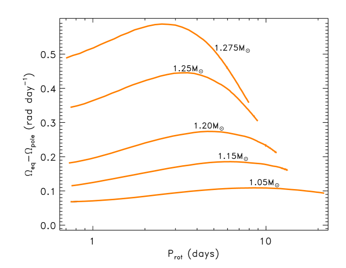
Figure 3: Surface differential rotation as a function of the rotation period for stars more massive than the sun.

Dwarf stars do not spin-down beyond a certain maximum rotation period depending on spectral type (see Fig. 1 of Rengarajan 1984). The dependence can be approximated by the linear function of the $B-V$ colour,

$$P_{\mathrm{rot}}^{\mathrm{max}}=109\left(B-V\right)-43\ \ \mathrm{day}.$$ (20)

Lines of Fig. 2 and 3 are terminated shortly beyond the maximum rotation period of Eq. (20).

The dependence of differential rotation on rotation rate is rather mild. Figures 2 and 3 show much stronger dependence on stellar mass, with more massive and hotter stars having larger differential rotation. The temperature dependence steepens as temperature increases. The dependence is in at least qualitative agreement with differential rotation measurements by Doppler imaging of Barnes et al. (2005) (for quantitative comparison of observed and computed rotation of young stars see Fig. 4 of Kitchatinov 2011). The line of Fig. 3 for the hottest star shows the $\Delta\Omega$ values slightly exceeding the largest differential rotation observed to date (Jeffers & Donati, 2008).

We used statistics of the results of Fig. 2 and 3 and also the results of computations for stellar masses intermediate between the lines of these Figures to define the coefficients of the regression (19). Only the results for rotation periods from slightly less than 1 day to $P_{\mathrm{rot}}^{\mathrm{max}}$ of Eq. (20) were included. Total statistics consists of about 1600 entries from differential rotation computations. The neural network (19) with $N=6$ gives quite a satisfactory approximation with a typical error of about 3%. Coefficients of the regression are given in Table 1.

Table 1: Coefficients of the neural network approximation (19) for the surface differential rotation in terms of the effective temperature and rotation period.

n	$W_{n}\left(\frac{\mathrm{rad}}{\mathrm{day}}\right)$	$w_{n}$	$w^{T}_{n}\left(K^{-1}\right)$	$w^{P}_{n}\left(\mathrm{day}^{-1}\right)$
$0$	$0.4521$	-	-	-
$1$	$0.1819$	$-3.573$	$5.075\times 10^{-4}$	$-3.118\times 10^{-2}$
$2$	$0.1063$	$2.532$	$-3.968\times 10^{-4}$	$0.1139$
$3$	$0.6062$	$-32.78$	$5.139\times 10^{-3}$	$-0.2310$
$4$	$0.1858$	$-18.55$	$2.993\times 10^{-3}$	$-5.674\times 10^{-2}$
$5$	$0.4596$	$17.90$	$-2.831\times 10^{-3}$	$0.4013$
$6$	$-0.1293$	$0.6043$	$-1.250\times 10^{-4}$	$1.206\times 10^{-3}$

Given the observed rotation period and temperature of a star, a theoretical prediction for the surface differential rotation can easily be estimated by using coefficients of this Table. It should be noted that the estimation applies to single main-sequence dwarfs only. It cannot be used for giants, close binaries, or pre-main sequence stars.

For a given mass, the amount of the surface differential rotation of Fig. 2 and 3 varies by about 30% as the rotation period changes. This mild variation is, however, worth discussing. The surface differential rotation increases initially up to a maximum but then decreases with $P_{\mathrm{rot}}$. Maxima on all lines are positioned at the values of the Coriolis number (7) between 10 and 20 (the Coriolis number is estimated for the middle of convection zone). Stars of smaller mass host slower convection with larger $\tau$ and attain their largest differential rotation at smaller rotation rates. The increase of differential rotation with angular velocity for not too rapid rotation was also found in 3D simulations of Brown et al. (2008). The 3D simulations predict, however, much larger differential rotation compared to our mean-field model.

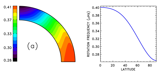
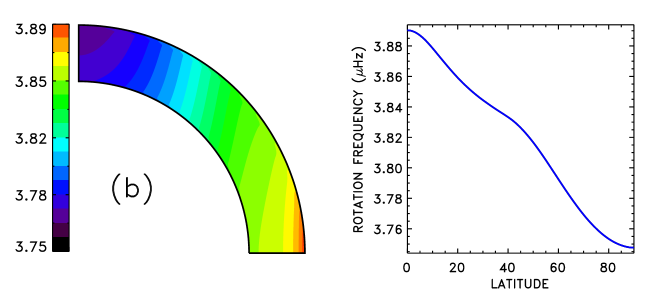
Figure 4: Angular velocity isolines in the convection zone and the angular velocity profile on the surface of $1M_{\odot}$ stars rotating with periods of 30 days (a) and 3 days (b).

The character of differential rotation changes between cases of slow ($\Omega^{*}<10$) and rapid ($\Omega^{*}>20$) rotation. Figure 4 shows the computed internal rotation of $1M_{\odot}$ stars rotating with periods of 30 and 3 days. The slow rotator has a smooth distribution of angular velocity on the surface and inside its convection zone. Isorotational surfaces are far from cylinders. The rapid rotator has thin boundary layers near the top and bottom of its convection zone. The layers result from violation of the Taylor-Proudman balance near the stress-free boundaries. The boundary layers were found in mean-field computations of Durney (1989) and Kitchatinov & Rüdiger (1999) as well as in 3D simulations of Brun & Toomre (2002) and Brown et al. (2008). The profile of angular velocity on the surface of the rapid rotator has a ‘peculiarity’ around the latitude where the angular velocity isoline tangential to the inner boundary at the equator arrives at the surface. Isorotational surfaces for the rapid rotator are much closer to cylinders.

Isorotational surfaces are cylinder-shaped near the equator and disk-shaped near the axis of rotation in all our computations. Isorotational surfaces are normal to the equatorial plane due to the symmetry of angular velocity distribution about the equator. As the distribution should be regular at the poles, isorotational surfaces are also normal to the rotation axis. Therefore, it is a general, though elementary rule, that isorotational surfaces are cylinder-shaped near the equator and disk-shaped near the poles (for an alternative opinion see Balbus 2009).

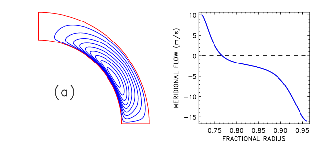
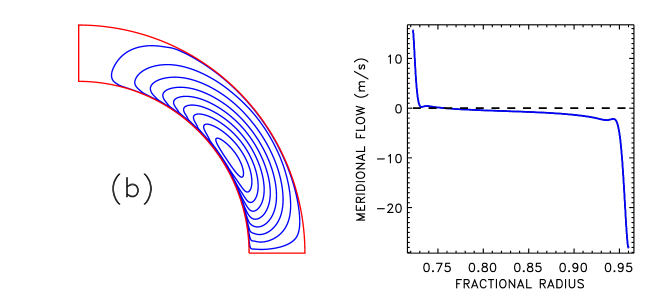
Figure 5: Meridional flow stream lines and the flow velocity as function of radius at the latitude of 45^∘ for $1M_{\odot}$ stars rotating with periods of 30 days (a) and 3 days (b). Negative velocity means poleward flow.

Violation of the Taylor-Proudman balance in the boundary layers results in relatively large values of the sources of meridional flow written on the right side of (10). Accordingly, the flow attains its largest velocities close to the boundaries. Figure 5 shows the meridional flow structure for the same computations as Fig. 4. The boundary layers in slow rotators are relatively thick (KO11). The flow is smoothly distributed over the entire thickness of the convection zone in this case. In a rapid rotator, however, the flow is confined in thin layers near the boundaries. This agrees with 3D simulations of Brown et al. (2008, 2010, 2011) who found a decrease of the meridional flow energy with rotation rate.

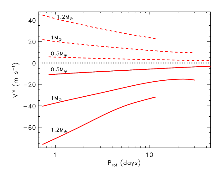
Figure 6: Dependence of meridional velocities on the top (full lines) and bottom of convection zone (dashed) on rotation period for stars of different mass. The velocities are taken at the latitude of 45^∘. Negative values mean poleward flow.

The near-boundary flows are significant. The surface flow is important because it is potentially observable. The flow near the bottom of the convection zone is increasingly recognized as important for dynamos (Choudhuri, 2011). Figure 6 shows how the near-boundary flows vary with stellar mass and rotation rate in our computations. The bottom flow is smaller but not much smaller compared to the surface. Note, however, that the flow does not penetrate deep beneath the convection zone. The meridional velocity decreases rapidly with depth below the convection zone (Gilman & Miesch, 2004). Similar to differential rotation, the flow amplitude increases with stellar mass and it increases steadily with rotation rate. The flow in the bulk of the convection zone, however, has the opposite tendency to decrease with rotation rate (Fig. 5).

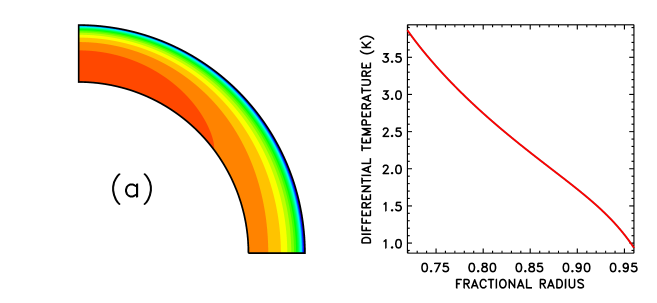
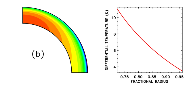
Figure 7: Entropy isolines and depth profiles of the pole-equator temperature difference (21) for $1M_{\odot}$ stars rotating with periods of 30 days (a) and 3 days (b).

The meridional flow is produced, in particular, by the effect of thermal wind due to the temperature dependence on latitude. Figure 7 shows the depth profiles of the ‘differential temperature’

$$\delta T(r)=\frac{T}{c_{\mathrm{p}}}\left(S(r,\theta)\mid_{\theta=0}-S(r,\theta)\mid_{\theta=\frac{\pi}{2}}\right)$$ (21)

for the same computations as Figs. 4 and 5. The differential temperature in mean-field models is produced partly by the dependence of thermal eddy conductivity on latitude but mainly by anisotropy of the thermal conductivity tensor (13) (Rüdiger et al., 2005). The anisotropy is induced by rotation and it increases with rotation rate. Accordingly, the differential temperature in faster rotating star of Fig. 7 is larger. There were many attempts to observe the small temperature difference between the equator and poles of the sun. Recent observations of Rast et al. (2008) suggest that the solar poles are warmer than the equator by about 2.5 K.

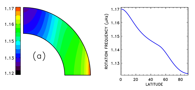
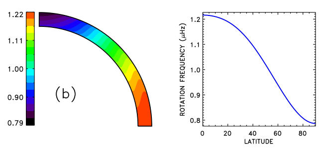
Figure 8: Differential rotation of $0.5M_{\odot}$ (a) and $1.2M_{\odot}$ (b) stars, both with $P_{\mathrm{rot}}=10$ days.

The anisotropy of thermal eddy conductivity is very important for differential rotation formation. It was not possible to reproduce the differential rotation of the sun neglecting this anisotropy (Rüdiger et al., 2005). Reducing the anisotropy, e.g., twice results in a change in the sense of differential rotation to an anti-solar state (the equator rotating slower than the poles) in slowly rotating stars. Only in this way were we able to reproduce a similar change in the sense of differential rotation found in the 3D simulations of Matt et al. (2011) and Bessolaz & Brun (2011).

Whether the differential rotation of a star belongs to the slow or rapid rotation regime is not solely controlled by the rotation period. Figure 8 compares the rotational states of $0.5M_{\odot}$ and $1.2M_{\odot}$ stars with the same $P_{\mathrm{rot}}=10$ days. The more massive star with $\Omega^{*}=3.7$ is a typical slow rotator while the smaller star with $\Omega^{*}=49$ is not.

4 Summary

Our main purpose was to predict the surface differential rotation in terms of measurable stellar parameters. This purpose is achieved by formulating the analytical approximation (19) for the differential rotation of main-sequence dwarfs as a function of their surface temperature and rotation period (Table 1 gives the coefficients of the approximation).

The prediction is based on the mean-field model of differential rotation (KO11), which relies on the quasi-linear theory of turbulent transport coefficients for rotating fluids (Rüdiger & Hollerbach, 2004). The results of extensive computations for stars of different mass and ages were processed using Gyrochronology (Barnes, 2003, 2007) and temperature scaling for differential rotation. The scaling means that the dependence of differential rotation on chemical composition and mass can be combined into a common dependence on temperature. The temperature scaling and Gyrochronology help to reduce the number of stellar parameters on which the differential rotation depends to just two - rotation period and temperature.

Our computations suggest that the main trend in the dependence of differential rotation on stellar parameters is its increase with effective temperature. The increase steepens for F-stars compared to cooler stars (Fig. 1) so that the maximum surface differential rotation, $\Delta\Omega\simeq 0.6$ rad day^-1, is achieved for the hottest F-stars we considered. There is also a weaker dependence on rotation rate, which is not monotonous. The surface differential rotation of young stars increases initially by about 30% as the star ages and rotation period increases but then it changes to a decrease with $P_{\mathrm{rot}}$. The maximum differential rotation is achieved at the values of the Coriolis number (7) between 10 and 20. This range of the Coriolis number separates the regimes of fast and slow rotation. Angular velocity distribution in slow rotators is smooth. Rapid rotators have thin boundary layers near the top and bottom of their convection zones where angular velocity and meridional flow vary sharply.

One-cell meridional flow with poleward flow on the surface and a return flow at the bottom of the convection zone was found in all our computations. The flow attains its maximum velocity on the top boundary. The amplitude of the flow increases with the effective temperature, but not as much as differential rotation does, and remains of an order of several tens of meters per second. The flow amplitude increases smoothly with rotation rate. The structure of the flow, however, changes considerably between cases of slow and fast rotation. The flow is distributed smoothly over depth in the convection zone in slow rotators. In rapid rotators, however, the flow is concentrated in the boundary layers near top and bottom with very weak meridional circulation in the bulk of the convection zone.

References

- Balbus (2009) Balbus S. A., 2009, MNRAS, 395, 2056
- Barnes et al. (2005) Barnes J. R., Collier Cameron A., Donati J.-F., James D. J., Marsden S. C., Petit P., 2005, MNRAS, 357, L1
- Barnes (2003) Barnes S. A., 2003, ApJ, 586, 464
- Barnes (2007) Barnes S. A., 2007, ApJ, 669, 1167
- Barnes (2010) Barnes S. A., 2010, ApJ, 722, 222
- Bessolaz & Brun (2011) Bessolaz N., Brun A. S., 2011, ApJ, 728, 115
- Brown et al. (2008) Brown B. P., Browning M. K., Brun A. S., Miesch M. S., Toomre J., 2008, ApJ, 689, 1354
- Brown et al. (2010) Brown B. P., Browning M. K., Brun A. S., Miesch M. S., Toomre J., 2010, ApJ, 711, 424
- Brown et al. (2011) Brown B. P., Miesch M. S., Browning M. K., Brun A. S., Toomre J., 2011, ApJ, 731, 69
- Brun & Toomre (2002) Brun A. S., Toomre J., 2002, ApJ, 570, 865
- Choudhuri (2011) Choudhuri A. R., 2011, in Proc IAU Symp. 273 Vol. 273, Origin of solar magnetism. pp 28–36
- Christensen-Dalsgaard & Houdek (2010) Christensen-Dalsgaard J., Houdek G., 2010, Ap&SS, 328, 51
- Collier Cameron (2003) Collier Cameron A., 2003, in S. Turcotte, S. C. Keller, & R. M. Cavallo ed., 3D Stellar Evolution Vol. 293 of ASPC, Stellar surface differential rotation from doppler imaging. p. 235
- Collier Cameron (2007) Collier Cameron A., 2007, Astron. Nachr., 328, 1030
- Collier Cameron et al. (2009) Collier Cameron A., Davidson V. A., Hebb L., et al. 2009, MNRAS, 400, 451
- Conway (1998) Conway A. J., 1998, New Astron. Rev., 42, 343
- Croll et al. (2006) Croll B., Walker G. A. H., Kuschnig et al. 2006, ApJ, 648, 607
- Donahue et al. (1996) Donahue R. A., Saar S. H., Baliunas S. L., 1996, ApJ, 466, 384
- Donati & Collier Cameron (1997) Donati J.-F., Collier Cameron A., 1997, MNRAS, 291, 1
- Durney (1989) Durney B. R., 1989, ApJ, 338, 509
- Gilman & Miesch (2004) Gilman P. A., Miesch M. S., 2004, ApJ, 611, 568
- Jeffers & Donati (2008) Jeffers S. V., Donati J.-F., 2008, MNRAS, 390, 635
- Käpylä & Brandenburg (2008) Käpylä P. J., Brandenburg A., 2008, A&A, 488, 9
- Käpylä et al. (2011) Käpylä P. J., Mantere M. J., Guerrero G., Brandenburg A., Chatterjee P., 2011, A&A, 531, A162
- Kitchatinov (2011) Kitchatinov L. L., 2011, ASInC, 2, 71
- Kitchatinov & Olemskoy (2011) Kitchatinov L. L., Olemskoy S. V., 2011, MNRAS, 411, 1059 (KO11)
- Kitchatinov et al. (1994) Kitchatinov L. L., Pipin V. V., Rüdiger G., 1994, Astron. Nachr., 315, 157
- Kitchatinov & Rüdiger (1995) Kitchatinov L. L., Rüdiger G., 1995, A&A, 299, 446
- Kitchatinov & Rüdiger (1999) Kitchatinov L. L., Rüdiger G., 1999, A&A, 344, 911
- Kitchatinov & Rüdiger (2005) Kitchatinov L. L., Rüdiger G., 2005, Astron. Nachr., 326, 379
- Kovári et al. (2004) Kovári Z., Strassmeier K. G., Granzer T., Weber M., Oláh K., Rice J. B., 2004, A&A, 417, 1047
- Küker et al. (2011) Küker M., Rüdiger G., Kitchatinov L. L., 2011, A&A, 530
- Lebedinskii (1941) Lebedinskii A. I., 1941, Astron. Zh., 18, 10
- Matt et al. (2011) Matt S. P., Do Cao O., Brown B. P., Brun A. S., 2011, Astronomische Nachrichten, 332, 897
- Meibom et al. (2009) Meibom S., Mathieu R. D., Stassun K. G., 2009, ApJ, 695, 679
- Miesch et al. (2006) Miesch M. S., Brun A. S., Toomre J., 2006, ApJ, 641, 618
- Miesch & Hindman (2011) Miesch M. S., Hindman B. W., 2011, ApJ, 743, 79
- Paxton (2004) Paxton B., 2004, PASP, 116, 699
- Rast et al. (2008) Rast M. P., Ortiz A., Meisner R. W., 2008, ApJ, 673, 1209
- Rengarajan (1984) Rengarajan T. N., 1984, ApJ, 283, L63
- Rüdiger (1989) Rüdiger G., 1989, Differential rotation and stellar convection. Gordon & Breach, New York
- Rüdiger et al. (2005) Rüdiger G., Egorov P., Kitchatinov L. L., Küker M., 2005, A&A, 431, 345
- Rüdiger & Hollerbach (2004) Rüdiger G., Hollerbach R., 2004, The magnetic universe. WILEY-VCH
- Schou et al. (1998) Schou J., Antia H. M., Basu S., et al. 1998, ApJ, 505, 390
- Skumanich (1972) Skumanich A., 1972, ApJ, 171, 565
- VandenBerg & Clem (2003) VandenBerg D. A., Clem J. L., 2003, AJ, 126, 778
- Walker et al. (2007) Walker G. A. H., Croll B., Kuschnig et al. 2007, ApJ, 659, 1611
- Weiss (1965) Weiss N. O., 1965, The Observatory, 85, 37
- Wilson et al. (1997) Wilson P. R., Burtonclay D., Li Y., 1997, ApJ, 489, 395