Entry and Spectrum Sharing Scheme Selection in Femtocell Markets^†

Abstract

Focusing on a femtocell communications market, we study the entrant network service provider’s (NSP’s) long-term decision: whether to enter the market and which spectrum sharing technology to select to maximize its profit. This long-term decision is closely related to the entrant’s pricing strategy and the users’ aggregate demand, which we model as medium-term and short-term decisions, respectively. We consider two markets, one with no incumbent and the other with one incumbent. For both markets, we show the existence and uniqueness of an equilibrium point in the user subscription dynamics, and provide a sufficient condition for the convergence of the dynamics. For the market with no incumbent, we derive upper and lower bounds on the optimal price and market share that maximize the entrant’s revenue, based on which the entrant selects an available technology to maximize its long-term profit. For the market with one incumbent, we model competition between the two NSPs as a non-cooperative game, in which the incumbent and the entrant choose their market shares independently, and provide a sufficient condition that guarantees the existence of at least one pure Nash equilibrium. Finally, we formalize the problem of entry and spectrum sharing scheme selection for the entrant and provide numerical results to complement our analysis.

I Introduction

Enhancing indoor wireless connectivity is a major challenge that hinders the proliferation of future-generation wireless networks operating at high frequencies, as signals at these frequencies suffer from severe fading and attenuation. Recently, femtocells (i.e., home base stations) have been proposed as an enabling solution to improve the indoor wireless communications service in 4G data networks [1]. Due to the wireless nature of femtocells, spectrum management for the coexistence of femtocells and macrocells is essential to realize the full potential of femtocells, which will be a key factor in the successful adoption of femtocells in the future communications market. Broadly speaking, there are three spectrum sharing schemes (or technologies) for the coexistence of femtocell and macrocell base stations [1]: (1) “split”: part of the spectrum owned by the NSPs is dedicated to femtocells; (2) “common”: the macrocell and the femtocells operate on the same spectrum and hence interfere with each other; (3) “partially shared”: the femtocells operate only on a fraction of the spectrum used by the macrocells. While these three spectrum sharing schemes have their respective advantages (e.g., spectrum efficiency, interference level), there is an ongoing debate over which scheme shall be adopted [2].

Figure 1: Three-stage decision-making problems of entrant and incumbent NSPs.

Because of the potential of significantly improving indoor communications services, femtocells are being adopted by more and more NSPs and meanwhile, create new business opportunities for start-ups which can enter the communications market by providing femtocell services. Thus, it is important to investigate whether or not it is profitable for an entrant NSP to enter a market with femtocell services and with which technologies (e.g., which spectrum sharing schemes). From an economics perspective, we study in this paper the problem of entry and spectrum sharing scheme selection faced by a profit-maximizing entrant network service provider (NSP) in a femtocells communications market. In particular, our study shall quantitatively characterize which spectrum sharing scheme shall be adopted by the entrant to maximize its profit and under which conditions. Two markets, one with no incumbent and the other with one incumbent, shall be investigated in this paper. Throughout the paper, we use “spectrum sharing scheme” and “technology” interchangeably wherever applicable. The structure of our analysis is shown in Fig. 1. Specifically, we consider a three-stage decision making process: in the long term, the entrant NSP, denoted by $\mathcal{S}_{2}$, makes entry and technology selection decisions to maximize its long-run profit; in the medium term, the incumbent NSP, denoted by $\mathcal{S}_{1}$, and NSP $\mathcal{S}_{2}$ make pricing (or market share) decisions to maximize their own revenue; and in the short term, users make subscription decisions to maximize their their own per-period utility. This three-stage hierarchical order of decision making can be explained as follows. Although dynamic spectrum management for femtocells has been proposed as a research thrust (e.g., [20]), deployment of a spectrum sharing scheme incurs a large cost, as it requires the network infrastructure and femtocell terminals to be manufactured in compliance with the chosen spectrum sharing scheme [2]. It also requires the support of protocol stacks, which is costly to develop. For instance, if “split” is chosen, then the femtocells terminals should be designed and manufactured such that they are only able to operate on certain bandwidths dedicated to femtocells. Therefore, the spectrum sharing scheme is difficult to change once deployed and hence, it is a long-term strategy for an NSP [2]. In contrast, an NSP can adjust its price over the lifespan of its network infrastructure, although the price cannot be updated as frequently as the users change their subscription decisions. Overall, we can assume that the users may change their subscription decisions frequently (e.g., a few days or weeks as a period), an NSP’s price is changed less frequently (e.g., several months or years as a period), while an NSP’s technology is a long-term decision (e.g., several years as a period). In order to evaluate and compare the long-term profitability of networks with different technologies, the entrant NSP needs to predict its maximum profit for each available technology. To maximize revenue given the technology and the associated cost, the NSP needs to know the users’ aggregate demand and their willingness to pay for the service, and then choose their optimal prices. Hence, we study first users’ dynamic decisions as to whether or not they subscribe to the entrant for communications services (i.e., the short-term problem), then revenue-maximizing pricing strategies (i.e., the medium-term problem), and finally entry and technology selection for the potential entrant (i.e., the long-term problem). A similar hierarchical analysis was considered in [3] in the contexts of Internet markets. Note that our study of user subscription dynamics provides a deeper understanding of the users’ subscription decisions than directly assuming a certain form of demand function (e.g., [3]), since our study characterizes both the dynamics and equilibrium point in the process of users’ subscription decisions.

When more users share the same network infrastructure, congestion effects are typically observed in communications networks and especially in wireless networks where interferences add to the difficulty in spectrum management [9][14]. In economics terms, congestion effects can be classified as a type of negative network externalities [27]. To capture congestion effects, we assume that the entrant provides each user with a QoS which is modeled as a non-increasing function in terms of the number of subscribers. In the first part of this paper, we focus on a market with no incumbent. By jointly considering the provided QoS and the charged price, users can dynamically decide whether or not to subscribe to the entrant. Under the assumption that users make their subscription decisions based on the most recent QoS and the current price, we show that, for any QoS function and price, there exists a unique equilibrium point of the user subscription dynamics at which the number of subscribers does not change. Given a spectrum sharing scheme, if the QoS degrades too fast when more users subscribe to the entrant, the user subscription dynamics may not converge to the equilibrium point. Hence, we find a sufficient condition for the QoS function to ensure the global convergence of the user subscription dynamics. We also derive upper and lower bounds on the optimal price and market share that maximize the entrant’s revenue. With linearly-degrading QoS functions (which we show can approximate very well the actual QoS functions), we obtain the optimal price in a closed form. Then, the entrant can select a technology out of its available options such that its long-term profit is maximized. Next, we turn to the analysis of a market with one incumbent in the second part of our paper. For the convenience of analysis, we assume that the incumbent has sufficient resources to provide each subscriber a guaranteed QoS (or to be more precise, a QoS that degrades sufficiently slowly such that it can be approximated as a constant without losing much accuracy). Given the provided QoS and the charged prices, users dynamically select the NSP that yields a higher (positive) utility. We first show that, for any prices, the considered user subscription dynamics always admits a unique equilibrium point, at which no user wishes to change its subscription decision. We next obtain a sufficient condition for the QoS functions to guarantee the convergence of the user subscription dynamics. Then, we analyze competition between the two NSPs. Specifically, modeled as a strategic player in a non-cooperative game, each NSP aims to maximize its own revenue by selecting its own market share while regarding the market share of its competitor as fixed. This is in sharp contrast with the existing related literature which typically studies price competition among NSPs. For the formulated market share competition game, we derive a sufficient condition on the QoS function that guarantees the existence of at least one pure Nash equilibrium (NE). Finally, we formalize the problem of entry and spectrum sharing scheme selection for the entrant, and complete our analysis by showing numerical results.

The rest of this paper is organized as follows. Section II reviews related work, and Section III describes the model. In Sections IV and V, we consider a market with no and with one incumbent, respectively, to study the user subscription dynamics and revenue maximization. The problem of technology selection is formalized in Section VI, and numerical results are shown in Section VII. Finally, concluding remarks are offered in Section VIII.

II Related Work

Recently, communications markets have been attracting an unprecedented amount of attention from various research communities, due to their rapid expansion. For instance, [2] compared the profitability of different spectrum sharing schemes in a femtocell market, whereas the user subscription dynamics and the problem of spectrum sharing scheme selection were neglected. In [3], the authors studied an Internet market and derived the optimal capacity investments for Internet service providers under various regulation policies. [4] studied technology adoption and competition between incumbent and emerging network technologies. Nevertheless, only constant QoS functions were considered in [4]. [5] investigated market dynamics emerging when next-generation networks and conventional networks coexist, by applying a market model that consists of content providers, NSPs, and users. Nevertheless, the level of QoS that a certain technology can provide was not considered in the model. In [6], the authors showed that non-cooperative communications markets suffer from unfair revenue distribution among NSPs and proposed a revenue-sharing mechanism that requires cooperation among NSPs. The behavior of users and its impact on the revenue distribution, however, were not explicitly considered in [6]. Without considering the interplay between different NSPs, the authors in [7] formulated a rate allocation problem by incorporating the participation of content providers into the model, and derived equilibrium prices and data rates. Another paper related to our work is [8] in which the authors examined the evolution of network sizes in wireless social community networks. A key assumption, based on which equilibrium was derived, is that a social community network provides a higher QoS to each user as the number of subscribers increases. While this assumption is valid if network coverage is the dominant factor determining the QoS or positive network externalities exist, it does not capture QoS degradation due to, for instance, user traffic congestion incurred at an NSP. [9] focused on a communications market with congestion costs and studied efficiency loss in terms of social welfare in both monopoly and oligopoly markets. However, an implicit assumption in [9] is that users are homogeneous in the sense that their valuations of QoS are the same. In [12], the authors considered users’ time-dependent utilities and proposed time-dependent pricing schemes that maximize either social welfare or the service provider’s revenue. Although congestion effects were taken into account, the convergence of the user subscription dynamics and competition between NSPs were not studied.

III Model

In this section, we provide a general model for the NSPs and users in a femtocell communications market. Note that in addition to femtocell markets, our model also applies to other communications markets such as cognitive radio markets.

III-A NSPs

Consider a femtocell market with one incumbent NSP and a potential entrant NSP, denoted by $\mathcal{S}_{1}$ and $\mathcal{S}_{2}$, respectively. In the paper, we focus on the entry and technology selection for the entrant. Thus, it is assumed that the incumbent NSP $\mathcal{S}_{1}$ has already deployed its technology, whereas the entrant NSP $\mathcal{S}_{2}$, if it decides to enter the market, can select a technology from its $L$ available options, denoted by $\{\mathcal{T}_{1},\mathcal{T}_{2},\cdots\mathcal{T}_{L}\}$, to maximize its long-term profit. It should be pointed out that we use $L$ instead of a specific integer to keep the model general. For the completeness of definition, we use $\mathcal{T}_{0}=\text{``Not Enter''}$ to represent that the entrant chooses not to enter the market, which yields zero long-term profit. In our considered scenario, a technology represents a spectrum sharing scheme and the available options for the entrant are “split”, “common”, and “partially shared” (or a subset of these three) in addition to “Not Enter”, whereas the decision of spectrum allocation (i.e., how much bandwidth allocated to femtocells and macrocells) is not explicitly considered in the paper. However, the spectrum allocation decision can be captured if we treat different spectrum allocations (but possibly with the same spectrum sharing scheme) as different technologies in the set $\{\mathcal{T}_{0},\mathcal{T}_{1},\mathcal{T}_{2},\cdots\mathcal{T}_{L}\}$. Moreover, we can also incorporate the entrant’s network capacity decision into our model by considering different capacities (but possibly with the same spectrum sharing scheme and/or spectrum allocation) as different technologies. Thus, a technology can be considered as a combination of resources (e.g., spectrum) and the way to utilize available resources. Note that, as we stated in Section I, technology selection is a long-term decision, while users’ subscription and NSPs’ pricing decisions are short-term and medium-term, respectively. Hence, the incumbent cannot change its technology regardless of whether the entrant enters the market or not [3]. We also assume that the incumbent NSP $\mathcal{S}_{1}$ has sufficient resources (e.g., network capacity) while the entrant NSP $\mathcal{S}_{2}$ does not. An example that fits into our assumptions on the NSPs is that the entrant is a small start-up. Hence, the QoS provided by the incumbent degrades much more slowly than that provided by the entrant and can be approximated as a constant without losing much accuracy (see Fig. 4 and its explanation for more details). On the other hand, as in [15][18] where the authors considered congestion effects because of limited resources, we consider that the QoS provided by the entrant NSP $\mathcal{S}_{2}$ degrades with the number of its subscribers. Let $\lambda_{i}$ be the fraction of users subscribing to NSP $\mathcal{S}_{i}$ for $i=1,2$. Then $\lambda_{1}$ and $\lambda_{2}$ satisfy $\lambda_{1},\lambda_{2}\geq 0$ and $\lambda_{1}+\lambda_{2}\leq 1$. Also, let $q_{i}$ be the QoS provided by NSP $\mathcal{S}_{i}$ for $i=1,2$. We assume that $q_{1}$ is independent of $\lambda_{1}$ while $q_{2}$ is non-increasing in $\lambda_{2}$. We use a function $g_{l}(\cdot)$ defined on $[0,1]$ to express the QoS provided by NSP $\mathcal{S}_{2}$ as $q_{2}=g_{l}(\lambda_{2})$, if NSP $\mathcal{S}_{2}$ selects $\mathcal{T}_{l}$ as its technology. We suppress the subscript $T_{l}$ when we analyze user subscription dynamics and NSP pricing decisions for notional convenience. Note that the QoS metric can be anything that users care about (e.g., throughput, delay, etc.). By considering average (normalized) throughput as the QoS metric, we shall discuss in Section VII how to derive the QoS function as a function of the number of subscribers. If the QoS is subject to multiple factors (e.g., throughput and delay), then we can express the QoS as a multi-variable function that takes into account all these factors.

III-B Users

There are a continuum of users that can potentially subscribe to one of the NSPs for communication services. The continuum model approximates well the real user population if there are a sufficiently large number of users in the market so that each individual user is negligible. As in [8][14], we assume throughout this paper that each user can subscribe to at most one NSP at any time instant. Users are heterogeneous in the sense that they may value the same level of QoS differently. Each user $k$ is characterized by a non-negative real number $\alpha_{k}$, which represents its valuation of QoS. Specifically, when user $k$ subscribes to NSP $\mathcal{S}_{i}$, its utility is given by

$$u_{k,i}=\alpha_{k}q_{i}-p_{i},$$ (1)

where $p_{i}$ is the subscription price charged by NSP $\mathcal{S}_{i}$, for $i=1,2$. Note that no other fees are charged by the NSPs. Users that do not subscribe to either of the two NSPs obtain zero utility. In (1), the product of the QoS and the valuation of QoS represents benefit received by a user and the price represents cost. We assume that a user’s utility is benefit from the service minus monetary cost. The unit of user $k$’s valuation of QoS (i.e., $\alpha_{k}$) is chosen such that $\alpha_{k}q_{i}$ has the same unit with that of the payment $p_{i}$, for $i=1,2$. Note that in our model the NSPs are allowed to engage in neither QoS discrimination nor price discrimination. That is, all users subscribing to the same NSP receive the same QoS and pay the same subscription price.

Now, we impose assumptions on the QoS function of NSP $\mathcal{S}_{2}$, user subscription decisions, and the users’ valuations of QoS as follows.

Assumption 1: For any technology $\mathcal{T}_{l}$, $l=1,2,\cdots,L$, $g(\cdot)$ is a non-increasing and continuously differentiable function, and $0<g(\lambda_{2})<q_{1}$ for all $\lambda_{2}\in[0,1]$.

Assumption 2: Each user $k$ subscribes to NSP $\mathcal{S}_{i}$ if $u_{k,i}>u_{k,j}$ and $u_{k,i}\geq 0$ for $i,j\in\{1,2\}$ and $i\not=j$. If $u_{k,1}=u_{k,2}\geq 0$, user $k$ subscribes to NSP $\mathcal{S}_{1}$.

Assumption 3: The users’ valuations of QoS follow a probability distribution whose probability density function (PDF) $f(\cdot)$ is strictly positive and continuous on $[0,\beta]$ for some $\beta>0$. For completeness of definition, we have $f(\alpha)=0$ for all $\alpha\notin[0,\beta]$. The cumulative density function (CDF) is given by $F(\alpha)=\int_{-\infty}^{\alpha}f(x)dx$ for all $\alpha\in\mathbb{R}$.

We briefly discuss the above three assumptions. Assumption 1 captures congestion effects that users experience when subscribing to NSP $\mathcal{S}_{2}$ with limited resources. Since NSP $\mathcal{S}_{1}$ has more resources than NSP $\mathcal{S}_{2}$, it is natural that $0<g(\lambda_{2})<q_{1}$ for $\lambda_{2}\in[0,1]$ (see Fig. 4 for illustration). Assumption 2 can be interpreted as a rational subscription decision. A rational user will subscribe to the NSP that provides a higher utility if at least one NSP provides a non-negative utility, and to neither NSP otherwise. Assumption 3 can be considered as an expression of user diversity in terms of the valuations of QoS. The lower bound on the interval is set as zero to simplify the analysis, and as considered in [2], this will be the case when there is enough diversity in the users’ valuations of QoS so that there are non-subscribers for any positive price.

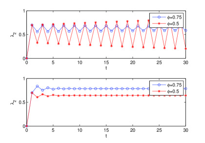
Figure 2: User subscription dynamics in a market with no incumbent. $u_{2,k}=\alpha_{k}\bar{q}_{2}-\delta\lambda_{2}+\beta\lambda_{2}^{\gamma}-p_{2}$. $p_{2}=0.3$, $\bar{q_{2}}=1.0$, $\delta=0.8$, and $\gamma=0.2$. $\delta=1.2$ (upper) and $\delta=0.8$ (lower).

III-C Assumptions and Remarks

In the following, we list important assumptions made in this paper to further clarify our model and the scenario that we focus on.

a. Constant QoS provided by the incumbent: The incumbent has sufficient (or over-provisioned) resources, such as available spectrum, and thus, it can provide a constant QoS to each user regardless of the number of subscribers.

b. No positive network externalities: The QoS provided by the entrant NSP is (weakly) decreasing in the number of its subscribers.

c. Lower QoS provided by the entrant than by the incumbent: The QoS provided by the entrant is lower than that provided by the incumbent.

d. Pricing-taking users: Users take the prices set by the NSPs as given, rather than anticipating the impacts of their decisions on the prices.

e. No switching cost: There is no cost, referred to as switching cost, incurred when users change their subscription decisions (see Section IV-A for more details).

Before proceeding with the analysis, we explain some of the assumptions in the following remarks.

Remark 1 (Constant QoS provided by the incumbent): Given sufficient resources, the QoS provided by the incumbent degrades sufficiently slowly such that it can be approximated as a constant without losing much accuracy (see Fig. 4 for more details). If the qualities of services provided by both the incumbent and the entrant are degrading as more users subscribe, then the price and the degradable QoS will jointly affect the users’ subscription decisions. Although the corresponding quantitative results will be different, the qualitative results remain unchanged. For example, the entrant NSP providing a uniformly lower QoS needs to charge a lower price in order to maximize its revenue.

Remark 2 (No positive network externalities): We note that compared to positive network externalities, negative network externalities are typically considered as dominating effects in wireless networking research, including femtocell research (e.g., [2]). For instance, when more users subscribe, congestion and interferences become intolerable, if the network resource (e.g., capacity) is not sufficient, and will significantly affect the users’ experiences. In general, suppressing the positive network externalities while only focusing on negative network effects (i.e., congestion effects) is a common approach in wireless networking and some operational research to studying the interaction among multiple network service providers (see, e.g., [2][3][9][10][14][15][16] and references therein). If positive network externalities are also taken into account in our model, there may exist multiple and possibly unstable equilibrium points in the user subscription dynamics. By considering the utility function $u_{i,k}=\alpha_{k}\bar{q}_{i}-\delta\lambda_{i}+\phi\lambda_{i}^{\gamma}-p_{i}$ for user $k$ where $0\leq\phi<\gamma$, $\gamma<1$, and $\phi\lambda_{i}^{\gamma}$ captures the positive network externalities), we show in Fig. 2 the user subscription dynamics with positive network externalities in a market with no incumbent. The details of specifying the user subscription dynamics are provided in Section IV-A. We see that if $\delta=0.8$ (i.e., not too large compared to $\bar{q}_{2}=1.0$, or the effects of negative externalities do not increase significantly when more users subscribe), then the convergence can be observed (from different starting points). Fig. 2 only shows a few instances for the ease of illustration, while more numerical results can be shown to support our statement. Note that, because of the term $\phi\lambda_{i}^{\gamma}$ with $\gamma<1$ representing the positive network externalities, we cannot theoretically guarantee the convergence starting from any initial points and given any charged price. Nevertheless, with $\gamma\geq 1$, it can be shown based on contraction mapping [24] that the existence of a unique equilibrium point and the convergence can be guaranteed for any charged price and any initial point $\lambda_{2}^{0}\in[0,1]$ if the condition

$$\left[{\max_{\alpha\in[0,\beta]}f(\alpha)}\right]\cdot\frac{\phi\gamma+\delta}{\bar{q}_{2}}<1$$ (2)

is satisfied. We see from (2) that $\delta$ cannot be too large given $\phi$ and $\gamma$. This is similar to our derived sufficient condition for the convergence of user subscription dynamics without positive network externalities. Similar results hold for the market with one incumbent, and are not shown here for brevity. A comprehensive investigation of the coexistence of both positive and negative network externalities will be left for our future work.

Remark 3 (Lower QoS provided by the entrant than by the incumbent): Given the three-stage decisions shown in Fig. 1, we implicitly assume that the NSP can afford any available technology at the beginning and hence, there is no need to “upgrade” the initially chosen technology afterwards. In general, there are two types of constraints – budget and technology – that limit the entrant’s technology selection. “No budget constraint” is assumed in the sense that the entrant can choose any technologies which are available for its selection. Thus, technology selection is primarily subject to the technology availability. Specifically, we focus on the case in which the technology available for the entrant is inferior to the incumbent’s in terms of QoS provisioning (i.e., $g(\lambda_{2})<q_{1}$ for $\lambda_{2}\in[0,1]$). In particular, in the case where the entrant has fewer resources than the incumbent (but the way to utilize the resources, e.g., spectrum sharing scheme, is the same), the QoS offered by the entrant will be lower than that offered by the incumbent (see, e.g., Fig. 4). This situation may arise in several practical scenarios. For example, if the incumbent is a wireless operator serving primary users while the incumbent operates a cognitive radio network serving secondary users that only opportunistically access to the “spectrum holes”. Another scenario is that upon the entrant’s entry into a femtocell market, only very limited spectrum is available, while the incumbent has already obtained a much larger range of spectrum. In each of these scenarios, we expect that the QoS provided by the entrant is not as good as the incumbent’s, even though the incumbent’s budget is sufficient to cover its entry and technology selection.

Remark 4 (Price-taking users): The assumption of price-taking users is reasonable when there are a sufficiently large number potential subscribers. In such cases, the impact of a single individual’s subscription decision on the decisions of the NSPs is negligible. In this paper, we use a continuum model to analyze the case of a sufficiently large number potential subscribers.

Remark 5 (Applicability of our model): Besides the femtocell market we focus on, our proposed model applies to a number of other communications markets. In particular, we can apply the model to study the spectrum acquisition decision (i.e., how much spectrum to purchase/lease from the spectrum owner) made by a small wireless carrier providing wireless cellular services, by a mobile virtual network operator (MVNO) [21] or by an entrant providing cognitive radio access services [22]. In such scenarios, the long-term “technology selection” in our model becomes “spectrum acquisition decision”, whereas the medium-term pricing decision and short-term user subscription decisions remain unaffected.

IV Femtocell Market With No Incumbent

In this section, we study user subscription dynamics and revenue maximization for the entrant in a femtocell market with no incumbent. In this scenario, the entrant becomes the monopolist in the market. In practice, this corresponds to an emerging market which an entrant tries to explore. We study first the user subscription dynamics and then the problem of revenue maximization, based on which the entrant can finally select its technology with which its profit is maximized.

IV-A User Subscription Dynamics

When the entrant NSP $\mathcal{S}_{2}$ operates in a market with no incumbent, each user has a choice of whether to subscribe to NSP $\mathcal{S}_{2}$ or not at each time instant. Since the QoS provided NSP $\mathcal{S}_{2}$ is varying with the fraction of its subscribers, each user will form a belief on the QoS of NSP $\mathcal{S}_{2}$ when it makes a subscription decision. To describe the dynamics of user subscription, we construct and analyze a dynamic model which specifies how users form their beliefs and make decisions based on their beliefs. We consider a discrete-time model with time periods indexed $t=1,2,\ldots$. At each period $t$, user $k$ holds a belief on the QoS of NSP $\mathcal{S}_{2}$, denoted by $\tilde{q}_{2,k}^{t}$ and the subscript $k$ denotes the user index, and makes a subscription decision to maximize its expected utility in the current period. Then, user $k$ subscribes to NSP $\mathcal{S}_{2}$ at period $t$ if and only if $\alpha_{k}\tilde{q}_{2,k}^{t}\geq p_{2}$. As in [4][8], an implicit assumption is that that, other than the subscription price, there is no cost involved in subscription decisions (e.g., initiation fees, termination fees, device prices). We specify that every user expects that the QoS in the current period is equal to that in the previous period. That is, we have $\tilde{q}_{2,k}^{t}=g(\lambda_{2}^{t-1})$ for $t=1,2,\ldots$, where $\lambda_{2}^{t}$ is the fraction of subscribers at period $t$.

By substituting $\tilde{q}_{2,k}^{t}=g(\lambda_{2}^{t-1})$ into $\alpha_{k}\tilde{q}_{2,k}^{t}\geq p_{2}$, we can see that user $k$ subscribes to NSP $\mathcal{S}_{2}$ if and only if $\alpha_{k}\geq\frac{p_{2}}{g(\lambda_{2}^{t-1})}$. That is, only those users with a valuation of QoS greater than or equal to $\frac{p_{2}}{g(\lambda_{2}^{t-1})}$ will subscribe to NSP $\mathcal{S}_{2}$ at time $t$. Thus, the fraction of subscribers of NSP $\mathcal{S}_{2}$ evolves following a sequence $\{\lambda_{2}^{t}\}_{t=0}^{\infty}$ in $[0,1]$ generated by

$$\lambda_{2}^{t}=h_{m}(\lambda_{2}^{t-1})\triangleq 1-F\left(\frac{p_{2}}{g(\lambda_{2}^{t-1})}\right),$$ (3)

for $t=1,2,\ldots$, starting from a given initial point $\lambda_{2}^{0}\in[0,1]$. Note that the price $p_{2}$ of NSP $\mathcal{S}_{2}$ is held fixed over time. Given the user subscription dynamics (3), we are interested in whether the fraction of subscribers will stabilize in the long run and, if so, to what value. As a first step, we define an equilibrium point of the user subscription dynamics.

Definition 1: $\lambda_{2}^{*}$ is an equilibrium point of the user subscription dynamics in the monopoly market of NSP $\mathcal{S}_{2}$ if it satisfies

$$h_{m}(\lambda_{2}^{*})=\lambda_{2}^{*}.$$ (4)

Definition 4 implies that once an equilibrium point is reached, the fraction of subscribers remains the same from that point on. Thus, equilibrium points are natural candidates for the long-run fraction of subscribers. The following Proposition, whose proof is deferred to to Appendix A, establishes the existence and uniqueness of an equilibrium point.

Proposition 1.

For any non-negative price $p_{2}$, there exists a unique equilibrium point of the user subscription dynamics in the market of NSP $\mathcal{S}_{2}$. $\square$

Although the analysis in this paper applies to a general QoS function $g(\lambda_{2})$, we consider a class of simple QoS functions defined below in order to obtain a closed-form expression of the equilibrium point and solve the revenue maximization problem explicitly.

Definition 2: The QoS function $g(\cdot)$ is linearly-degrading if $g(\lambda_{2})=\bar{q}_{2}-c\lambda_{2}$ for all $\lambda_{2}\in[0,1]$, for some $\bar{q}_{2}>0$ and $c\in[0,\bar{q}_{2})$. In particular, a linearly-degrading QoS function with $c=0$, i.e., $g(\lambda_{2})=\bar{q}_{2}$ for all $\lambda_{2}\in[0,1]$, is referred to as a constant QoS function.

Linearly-degrading QoS functions model a variety of applications including flow control in [13] and capacity sharing in [15]. More importantly, it can be viewed as an affine approximation of real QoS functions and we shall see in the numerical results that the affine approximation is reasonably close to the actual QoS functions. With a linearly-degrading QoS function and uniformly distributed valuations of QoS, we can obtain a simple closed-form expression of the equilibrium point. Specifically, with $g(\lambda_{2})=\bar{q}_{2}-c\lambda_{2}$ for $\lambda_{2}\in[0,1]$ and $f(\alpha)=1/\beta$ for $\alpha\in[0,\beta]$, the equilibrium point of the user subscription dynamics in the market of NSP $\mathcal{S}_{2}$ can be expressed as a function of $p_{2}$ as follows:

$$\lambda_{2}^{*}(p_{2})=\left\{\begin{matrix}\frac{\bar{q}_{2}+c-\sqrt{(\bar{q}_{2}-c)^{2}+\frac{4cp_{2}}{\beta}}}{2c},&&\hfill\text{for }p_{2}\in[0,\beta\bar{q}_{2}],\\ 0,\hfill&&\hfill\text{for }p_{2}\in(\beta\bar{q}_{2},\infty),\end{matrix}\right.$$ (5)

if $c\in(0,\bar{q}_{2})$, and $\lambda_{2}^{*}(p_{2})=\max\{0,1-p_{2}/(\beta\bar{q}_{2})\}$ if $c=0$.

Our equilibrium analysis so far guarantees the existence of a unique stable point of the user subscription dynamics. However, it does not discuss whether the unique stable point will be eventually reached. To answer this question, we turn to the analysis of the convergence properties of the user subscription dynamics. The convergence of the user subscription dynamics is not always guaranteed, especially when the QoS provided by the monopolist degrades rapidly with respect to the fraction of subscribers. As a hypothetical example, suppose that only a small fraction of users subscribe to NSP $\mathcal{S}_{2}$ at period $t$ and each subscriber obtains a high QoS. In our model of belief formation, users expect that the QoS will remain high at period $t+1$, and thus a large fraction of users subscribe at period $t+1$, which will result in a low QoS at period $t+1$. This in turn will induce a small fraction of subscribers at period $t+2$. When the QoS is very sensitive to the fraction of subscribers, the user subscription dynamics may oscillate around or diverge away from the equilibrium point and thus convergence may not be obtained. The following theorem provides a sufficient condition under which the user subscription dynamics always converges.

Theorem 1.

For any non-negative price $p_{2}$, the user subscription dynamics specified by (3) converges to the unique equilibrium point starting from any initial point $\lambda_{2}^{0}\in[0,1]$ if

$$\max_{\lambda_{2}\in[0,1]}\left\{-\frac{g^{\prime}(\lambda_{2})}{g(\lambda_{2})}\right\}<\frac{1}{K},$$ (6)

where $K=\max_{\alpha\in[0,\beta]}f(\alpha)\alpha$.

Proof.

See Appendix B. $\square$

By applying Theorem 1 to linearly-degrading QoS functions, we obtain the following result.

Corollary 1.

If the QoS function $g(\cdot)$ is linearly-degrading, i.e., $g(\lambda_{2})=\bar{q}_{2}-c\lambda_{2}$ for $\lambda_{2}\in[0,1]$, and

$$\frac{c}{\bar{q}_{2}}<\frac{1}{1+K}$$ (7)

where $K=\max_{\alpha\in[0,\beta]}f(\alpha)\alpha$, then the user subscription dynamics converges to the unique equilibrium point starting from any initial point $\lambda_{2}^{0}\in[0,1]$. $\square$

The condition (6) in Theorem 1 is sufficient but not necessary for the convergence of the user subscription dynamics. In particular, we observe through numerical simulations that in some cases (e.g., $g(\lambda_{2})=1-0.9\lambda_{2}$ for $\lambda_{2}\in[0,1]$ and $f(\alpha)=1$ for $\alpha\in[0,1]$) the user subscription dynamics converges for a wide range of prices although the condition (6) is violated. Nevertheless, the sufficient condition provides us with the insight that if QoS degradation is too fast (i.e., $-Kg^{\prime}(\lambda_{2})$ is larger than $g(\lambda_{2})$ for some $\lambda_{2}\in[0,1]$), the dynamics may oscillate or diverge. If our analysis is applied to study the spectrum acquisition decision, a practical implication of the derived convergence condition (which may also be mapped into the spectrum requirement) is that the acquired spectrum should be sufficiently large such that the congestion does not grow too rapidly when more users subscribe [19].

We set up our basic model by assuming that all the users will simultaneously make their subscription decisions at the beginning of each decision period, i.e., “simultaneous/synchronous move”. However, it should be noted that we can generalize the user subscription dynamics by assuming that only $\epsilon$ fraction of users, where $\epsilon\in(0,1]$, change their subscription decisions in each period. In this generalized scenario, not all the users make their decisions simultaneously, while only $\epsilon$ fraction of users in the market do. We still assume that all the users that change their subscription decisions expect that the QoS they receive in the next time period will be the same as that in the current time period. This can be viewed as “asynchronous move”, under which the user subscription dynamics is generated by

$$\lambda_{2}^{t}=(1-\epsilon)\lambda_{2}^{t-1}+\epsilon h_{m}(\lambda_{2}^{t-1})$$ (8)

for $t=1,2,\ldots$, starting from an initial point $\lambda_{2}^{0}\in[0,1]$. For the more general user subscription dynamics in 8, our original existence and uniqueness analysis is still valid, whereas the convergence analysis (Theorem 1) is affected and the sufficient convergence condition is modified as

$$\max_{\lambda_{2}\in[0,1]}\left\{-\frac{g^{\prime}(\lambda_{2})}{g(\lambda_{2})}\right\}<\frac{1}{\epsilon K}.$$ (9)

As the condition (9) is more easily satisfied for a smaller $\epsilon$, we see that there is a trade-off between the guarantee of convergence and the speed of convergence. There exist other dynamics, such as continuous-time dynamics, modeling the user subscription process and interested readers may refer to [4] for a detailed analysis.

Next, we discuss the cost involved when users change their subscription decisions. For simplicity, we assume that the costs of activating and terminating the subscription are the same, and we refer to this cost as switching cost denoted by $c_{s}$, which includes, but is not limited to, time spent in calling the customer service, activation fees and early termination fees. By charging this cost, the NSP creates the effect of user “lock-in”, which we note may result in multiple equilibrium points and different convergence behaviors, subject to the initial point. For instance, in the extreme case in which the cost is so high (e.g., greater than $\beta g(0)$ which is the highest benefit that a user can possibly gain by subscribing to NSP $\mathcal{S}_{2}$) that no users would like to change their subscription decisions, every possible value of $\lambda_{2}\in[0,1]$ is an equilibrium point. In general, if user $k$ is a subscriber in the time period $t$, it will continue the subscription in the next time period $t+1$ if

$$\begin{split}\alpha_{k}g(\lambda_{2}^{t})-p_{2}\geq-c_{s}.\end{split}$$ (10)

On the other hand, if user $k$ is not a subscriber in the time period $t$, it will choose to subscribe to the NSP in the next time period $t+1$ if

$$\begin{split}\alpha_{k}g(\lambda_{2}^{t})-p_{2}-c_{s}\geq 0.\end{split}$$ (11)

While rigorous analysis of $c_{s}$ is left as our future work, we show in Fig. 3 the impact of switching cost $c_{s}$ on the users’ subscription decisions. The upper plot indicates that switching costs may make the user subscription dynamics converge even though the QoS degrades rapidly such that the user subscription dynamics does not converge without switching costs. We explain this point by noting that, with switching costs, fewer users will change their subscription decisions and hence the user subscription dynamics converges under milder conditions. With switching costs imposed, it can also be seen from Fig. 3 that there may exist multiple equilibria in the user subscription dynamics and the equilibrium, to which the user subscription dynamics converges, depends on the initial point. Since the analysis of the NSP’s pricing decision and technology selection largely relies on the equilibrium point of the user subscription dynamics, the existence of multiple equilibrium points is challenging to deal with and loses mathematical tractability. Thus, as in the existing related literature (e.g., [4][8][15]), the switching cost is not considered in our paper. Moreover, neglecting the switching cost is particularly applicable in a setting where handover and service provider selection in real time are possible.

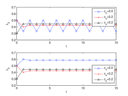
Figure 3: User subscription dynamics in a market with no incumbent. $p_{2}=0.4$. For $\lambda_{2}\in[0,1]$, $g(\lambda_{2})=1.2-1.2\lambda_{2}$ (upper) and $g(\lambda_{2})=1.2-0.4\lambda_{2}$ (lower).

IV-B Revenue Maximization

Building on the equilibrium analysis of the user subscription dynamics, we are now interested in finding an optimal price of NSP $\mathcal{S}_{2}$ that maximizes its equilibrium revenue in the market with no incumbent. Note that the optimal revenue is associated with the technology selected by NSP $\mathcal{S}_{2}$. To keep the notion succinct, we omit the subscript of $\mathcal{T}_{l}$ in the revenue and express it as

$$R_{2}(p_{2})=p_{2}\lambda_{2}^{*}(p_{2}),$$ (12)

where $\lambda_{2}^{*}(p_{2})$ is the equilibrium point of the user subscription dynamics at price $p_{2}$. It can be shown that $\lambda_{2}^{*}(0)=1$, $\lambda_{2}^{*}(\cdot)$ is strictly decreasing on $[0,\beta g(0)]$, and $\lambda_{2}^{*}(p_{2})=0$ for all $p_{2}\geq\beta g(0)$, where $\beta$ is the maximum valuation of QoS of all the users. As a result, NSP $\mathcal{S}_{2}$ will gain a positive revenue only if it sets a price $p_{2}$ in $(0,\beta g(0))$, and thus a revenue-maximizing price lies in $(0,\beta g(0))$. However, it is difficult to directly obtain an explicit expression of $p_{2}\in(0,\beta g(0))$ that maximizes $R_{2}(p_{2})$ even when the QoS function is linearly-degrading and the users’ valuations of QoS are uniformly distributed, since $\lambda_{2}^{*}(p_{2})$ is a complicated function of $p_{2}$ as can be seen in (5). In the following analysis, we reformulate the revenue maximization problem by applying the marginal user principle [17][18]. Specifically, we change the choice variable in the revenue maximization problem.

Suppose that a marginal user exists, whose valuation of QoS is denoted by $\alpha$. Then from the utility function in (1), we can see that all the users with valuations of QoS greater than $\alpha$ receive a positive utility and thus subscribe to NSP $\mathcal{S}_{2}$ [2][17]. Hence, when a marginal user has a valuation of QoS $\alpha\in[0,\beta]$, the fraction of subscribers is given by $\lambda_{2}=1-F(\alpha)$. Also, for a given price $p_{2}\in[0,\beta g(0)]$, there exists a unique valuation of QoS of a marginal user $\alpha\in[0,\beta]$, and the relationship between $p_{2}$ and $\alpha$ is given by

$$p_{2}=\alpha g(1-F(\alpha)).$$ (13)

Based on the above relationships between $p_{2}$, $\alpha$, and $\lambda_{2}$, we can formulate the revenue maximization problem using different choice variables as follows:

$$\begin{split}\max_{p_{2}\in[0,\beta g(0)]}p_{2}\lambda_{2}^{*}(p_{2})&=\max_{\alpha\in[0,\beta]}\alpha g(1-F(\alpha))\left[1-F(\alpha)\right]\\ &=\max_{\lambda_{2}\in[0,1]}F^{-1}(1-\lambda_{2})g(\lambda_{2})\lambda_{2},\end{split}$$ (14)

where $F^{-1}(\cdot)$ is the inverse function of $F(\cdot)$ defined on $[0,1]$. It is clear that a solution to each of the above three problems exists, since the constraint set is compact and the objective function is continuous. Let $p^{*}$, $\alpha^{*}$, and $\lambda_{2}^{**}$ be a solution to each respective problem in (14). By imposing an assumption on the distribution of the users’ valuations of QoS, we obtain upper and lower bounds on $p^{*}$, $\alpha^{*}$, and $\lambda_{2}^{**}$ in Proposition 2, whose proof is given in Appendix C.

Proposition 2.

Suppose that $f(\cdot)$ is non-increasing on $[0,\beta]$. Then optimal variables solving the revenue maximization problem in (14) satisfy $F^{-1}(1/2)g(1/2)\leq p_{2}^{*}<\beta g(0)$, $F^{-1}(1/2)\leq\alpha^{*}<\beta$, and $0<\lambda_{2}^{**}\leq 1/2$. $\square$

The non-increasing property of $f(\cdot)$ can be considered as representing a class of emerging markets where there are fewer users with higher valuations of QoS provided by the NSP [27]. Proposition 2 shows that when the monopolist maximizes its revenue in an emerging market, no more than a half of the users, only those whose valuations are sufficiently high, are served. In other words, in an emerging market, the NSP will serve a minority of users with high valuations to maximize its revenue. Since a uniform distribution satisfies the non-increasing property, applying Proposition 2 to the case of a uniform distribution of the users’ valuations of QoS (i.e., $f(\alpha)=1/\beta$ and $F(\alpha)=\alpha/\beta$ for $\alpha\in[0,\beta]$) yields $(\beta/2)g(1/2)\leq p_{2}^{*}<\beta g(0)$ and $\beta/2\leq\alpha^{*}<\beta$. If, in addition, the QoS function satisfies the sufficient condition (6) for convergence, we obtain tighter bounds on optimal variables.

Corollary 2.

Suppose that $f(\alpha)=1/\beta$ for $\alpha\in[0,\beta]$ and $-g^{\prime}(\lambda_{2})/g(\lambda_{2})<1$ for all $\lambda_{2}\in[0,1]$. Then optimal variables solving the revenue maximization problem in (14) satisfy $(\beta/2)g(1/2)\leq p_{2}^{*}<[(\sqrt{5}-1)/2]\beta g((3-\sqrt{5})/2)$, $\beta/2\leq\alpha^{*}<[(\sqrt{5}-1)/2]\beta$, and $(3-\sqrt{5})/2<\lambda_{2}^{**}\leq 1/2$.

Proof.

The proof is omitted due to space limitations. $\square$

With a uniform distribution of the users’ valuations of QoS and a linearly-degrading QoS function, we can obtain explicit expressions of optimal variables of the revenue maximization problem as follows:

$$\alpha^{*}=\frac{2c-\bar{q}_{2}+\sqrt{\bar{q}_{2}^{2}+c^{2}-c\bar{q}_{2}}}{3c}\beta,$$ (15)

$$\lambda_{2}^{**}=\frac{c+\bar{q}_{2}-\sqrt{\bar{q}_{2}^{2}+c^{2}-c\bar{q}_{2}}}{3c},$$ (16)

and $p_{2}^{*}=\alpha^{*}(\bar{q}_{2}-c\lambda_{2}^{**})$. The high-level insight from this result is that the optimal price maximizing the NSP’s revenue should be decreased if the QoS degrades more quickly and that the optimal market share is independent of the interval on which the users’ valuation of QoS is uniformly distributed. Moreover, the result quantifies the impacts of the QoS function (i.e., maximum QoS and degrading rate) as well as the users’ valuation of QoS on the optimal price. For instance, as shown in Fig. 5(a), the NSP does not incur a significant revenue loss if its equilibrium market share is around one half, whereas its revenue loss is nearly 10% and more if its equilibrium market share is less than 0.4 or greater than 0.6. This indicates that the NSP’s revenue is near to its optimum if the NSP serves around one half of the market, while both under-serving and over-serving will significantly reduce the NSP’s revenue. Due to the implicit and explicit coupling involved in our considered three-decision making process, it is difficult to see how the quantitative results in the pricing decision stage directly affects the entrant’s long-term technology selection. Nevertheless, solving the revenue maximization problem (i.e., medium-term problem) explicitly serves as a basis for the entrant to decide whether or not to enter the market and select the technology that maximizes its long-term profit (i.e., long-term problem).

Finally, we note that in order to maximize its equilibrium revenue, the entrant needs to know the distribution of the users’ valuations of QoS by conducting market surveys and using data-mining and learning techniques. The details of information acquisition are beyond the scope of this paper.

V Femtocell Market With One Incumbent

In this section, we analyze user subscription dynamics and market competition for the entrant in a femtocel market with one incumbent. In other words, the two NSPs operate and compete against each other in a duopoly market.

V-A User Subscription Dynamics

With the two NSPs operating in the market, each user has three possible choices at each time instant: subscribe to NSP $\mathcal{S}_{1}$, subscribe to NSP $\mathcal{S}_{2}$, and subscribe to neither. As in the market with no incumbent, we consider a dynamic model in which the users update their beliefs and make subscription decisions at discrete time period $t=1,2,\ldots$. The users expect that the QoS provided by NSP $\mathcal{S}_{2}$ in the current period is equal to that in the previous period and make their subscription decisions to maximize their expected utility in the current period [8]. We assume that, other than the subscription price, there is no cost involved in subscription decisions (e.g., initiation fees, termination fees) when users switch between NSP $\mathcal{S}_{1}$ and NSP $\mathcal{S}_{2}$ [4]. By Assumption 2, at period $t=1,2\cdots$, user $k$ subscribes to NSP $\mathcal{S}_{1}$ if and only if

$$\alpha_{k}q_{1}-p_{1}\geq\alpha_{k}g(\lambda_{2}^{t-1})-p_{2}\text{ and }\alpha_{k}q_{1}-p_{1}\geq 0,$$ (17)

to NSP $\mathcal{S}_{2}$ if and only if

$$\alpha_{k}g(\lambda_{2}^{t-1})-p_{2}>\alpha_{k}q_{1}-p_{1}\text{ and }\alpha_{k}g(\lambda_{2}^{t-1})-p_{2}\geq 0,$$ (18)

and to neither NSP if and only if

$$\alpha_{k}q_{1}-p_{1}<0\text{ and }\alpha_{k}g(\lambda_{2}^{t-1})-p_{2}<0.$$ (19)

By solving (17)–(19), it can be shown that, given the prices $(p_{1},p_{2})$, the user subscription dynamics is described by a sequence $\{(\lambda_{1}^{t},\lambda_{2}^{t})\}_{t=0}^{\infty}$ in $\Lambda=\{(\lambda_{1},\lambda_{2})\in\mathbb{R}_{+}^{2}\;|\;\lambda_{1}+\lambda_{2}\leq 1\}$ generated by

$$\lambda_{1}^{t} =h_{d,1}(\lambda_{1}^{t-1},\lambda_{2}^{t-1})\triangleq 1-F\left(\frac{p_{1}-p_{2}}{q_{1}-g(\lambda_{2}^{t-1})}\right),$$ (20)

$$\lambda_{2}^{t} =h_{d,2}(\lambda_{1}^{t-1},\lambda_{2}^{t-1})\triangleq F\left(\frac{p_{1}-p_{2}}{q_{1}-g(\lambda_{2}^{t-1})}\right)-F\left(\frac{p_{2}}{g(\lambda_{2}^{t-1})}\right)$$ (21)

if $p_{1}/q_{1}>p_{2}/g(\lambda_{2}^{t-1})$, and by

$$\lambda_{1}^{t} =h_{d,1}(\lambda_{1}^{t-1},\lambda_{2}^{t-1})\triangleq 1-F\left(\frac{p_{1}}{q_{1}}\right),$$ (22)

$$\lambda_{2}^{t} =h_{d,2}(\lambda_{1}^{t-1},\lambda_{2}^{t-1})\triangleq 0$$ (23)

if $p_{1}/q_{1}\leq p_{2}/g(\lambda_{2}^{t-1})$, for $t=1,2,\ldots$, starting from a given initial point $(\lambda_{1}^{0},\lambda_{2}^{0})$. Note that there are two regimes of the user subscription dynamics, and which regime governs the dynamics depends on the relative values of the prices per QoS, i.e., $p_{1}/q_{1}$ and $p_{2}/g(\lambda_{2}^{t-1})$. Specifically, if the price per QoS offered by NSP $\mathcal{S}_{1}$ is higher than that offered by NSP $\mathcal{S}_{2}$ (i.e., $p_{1}/q_{1}>p_{2}/g(\lambda_{2}^{t-1})$), then users who are sensitive to prices (i.e., those whose valuations are not sufficiently high and lie between $\frac{p_{1}-p_{2}}{q_{1}-g(\lambda_{2}^{t-1})}$ and $\frac{p_{2}}{g(\lambda_{2}^{t-1})}$) will prefer NSP $\mathcal{S}_{2}$ to NSP $\mathcal{S}_{1}$.

We give the definition of an equilibrium point, which is similar to Definition 1.

Definition 3: $(\lambda_{1}^{*},\lambda_{2}^{*})$ is an equilibrium point of the user subscription dynamics in duopoly the market of NSP $\mathcal{S}_{1}$ and $\mathcal{S}_{2}$ if it satisfies

$$h_{d,1}(\lambda_{1}^{*},\lambda_{2}^{*})=\lambda_{1}^{*}\text{ and }h_{d,2}(\lambda_{1}^{*},\lambda_{2}^{*})=\lambda_{2}^{*}.$$ (24)

We establish the existence and uniqueness of an equilibrium point and provide equations characterizing it in Proposition 3, whose proof is deferred to Appendix D.

Proposition 3.

For any non-negative price pair $(p_{1},p_{2})$, there exists a unique equilibrium point $(\lambda_{1}^{*},\lambda_{2}^{*})$ of the user subscription dynamics in the market with one incumbent. Moreover, $(\lambda_{1}^{*},\lambda_{2}^{*})$ satisfies

$$\left\{\begin{split}\lambda_{1}^{*}=1-F\left(\frac{p_{1}}{q_{1}}\right)\text{, }\lambda_{2}^{*}=0,\;\;\;\;\;\;\;\;\;\;\;\;\;\;\;\;\;\;\;\;\text{ if }\frac{p_{1}}{q_{1}}\leq\frac{p_{2}}{g(0)},\\ \lambda_{1}^{*}=1-F\left(\theta_{1}^{*}\right)\text{, }\lambda_{2}^{*}=F\left(\theta_{1}^{*}\right)-F\left(\theta_{2}^{*}\right),\;\;\;\text{if }\frac{p_{1}}{q_{1}}>\frac{p_{2}}{g(0)},\end{split}\right.$$ (25)

where $\theta_{1}^{*}=(p_{1}-p_{2})/(q_{1}-g(\lambda_{2}^{*}))$ and $\theta_{2}^{*}=p_{2}/g(\lambda_{2}^{*})$. $\square$

Proposition 3 indicates that, given any prices $(p_{1},p_{2})$, the market shares of the two NSPs are uniquely determined when the fraction of users subscribing to each NSP no longer changes. Theoretically, this result ensures that if the NSPs choose the optimal price (and also the entrant NSP selects the optimal technology), then their corresponding profits will be maximized, since the resulting outcome (e.g., equilibrium) is unique and the NSPs face no uncertainty in the user subscription dynamics. Proposition 3 also shows that the structure of the equilibrium point depends on the relative values of $p_{1}/q_{1}$ and $p_{2}/g(0)$. Specifically, if the price per QoS of NSP $\mathcal{S}_{1}$ is always lower than or equal to that of NSP $\mathcal{S}_{2}$, i.e., $p_{1}/q_{1}\leq p_{2}/g(0)$, then no users subscribe to NSP $\mathcal{S}_{2}$ at the equilibrium point. On the other hand, if NSP $\mathcal{S}_{2}$ offers a lower price per QoS to its first subscriber than NSP $\mathcal{S}_{1}$ does, i.e., $p_{1}/q_{1}>p_{2}/g(0)$, then both NSP $\mathcal{S}_{1}$ and NSP $\mathcal{S}_{2}$ may attract a positive fraction of subscribers. This result regarding the price per QoS quantifies the necessary condition on prices that the entrant NSP should set such that it can receive a positive revenue. We note that, although it may be familiar to researchers and/or managers, this result is important and relevant for the completeness of study, as it rigorously characterizes the equilibrium outcome in the user subscription dynamics and serves as the basis for both NSPs to make pricing decisions and for the entrant to make technology decisions. The importance of Proposition 3 can also be reflected in recent works (e.g., [4][8][15][2]) which establish similar results under various settings.

We now investigate whether the user subscription dynamics specified by (20)–(23) stabilizes as time passes. As in the market with no incumbent, the considered user subscription dynamics is guaranteed to converge to the unique equilibrium when the QoS degradation of NSP $\mathcal{S}_{2}$ is not too fast. In the following theorem, we provide a sufficient condition for convergence.

Theorem 2.

For any non-negative price pair $(p_{1},p_{2})$, the user subscription dynamics specified by (20)–(23) converges to the unique equilibrium point starting from any initial point $(\lambda_{1}^{0},\lambda_{2}^{0})\in\Lambda$ if

$$\max_{\lambda_{2}\in[0,1]}\left\{-\frac{g^{\prime}(\lambda_{2})}{g(\lambda_{2})}\cdot\frac{q_{1}}{q_{1}-g(\lambda_{2})}\right\}<\frac{1}{K},$$ (26)

where $K=\max_{\alpha\in[0,\beta]}f(\alpha)\alpha.$

Proof.

See Appendix E. $\square$

Note that the condition (26) imposes a more stringent requirement on the QoS function $g(\cdot)$ than the condition (6) does, since $q_{1}/(q_{1}-g(\lambda_{2}))>1$ for all $\lambda_{2}\in[0,1]$. However, the condition (26) provides us with a similar insight that, if QoS degradation is severe, the user subscription dynamics may exhibit oscillation or divergence.

V-B Revenue Maximization

We now study revenue maximization in the market with one incumbent. In the economics literature, competition among a small number of firms has been analyzed using game theory, following largely two distinct approaches: Bertrand competition and Cournot competition [25]. In Bertrand competition, firms choose prices independently while supplying quantities demanded at the chosen prices. On the other hand, in Cournot competition, firms choose quantities independently while prices are determined in the markets to equate demand with the chosen quantities. In the case of monopoly, whether the monopolist chooses the price or the quantity does not affect the outcome since there is a one-to-one relationship between the price and the quantity given a downward-sloping demand function. This point was illustrated with our model in Section IV-B. On the contrary, in the presence of strategic interaction, whether firms choose prices or quantities can affect the outcome significantly. For example, it is well-known that identical firms producing a homogeneous good obtain zero profit in the equilibrium of Bertrand competition while they obtain a positive profit in the equilibrium of Cournot competition, if they have a constant marginal cost of production and face a linear demand function.

We first consider Bertrand competition between the two NSPs. Let $\lambda_{i}^{*}(p_{1},p_{2})$ be the market share of NSP $\mathcal{S}_{i}$, for $i=1,2$, at the unique equilibrium point of the considered user subscription dynamics given a price pair $(p_{1},p_{2})$. $\lambda_{i}^{*}(\cdot)$ can be interpreted as a demand function of NSP $\mathcal{S}_{i}$, and the revenue of NSP $\mathcal{S}_{i}$ at the equilibrium point can be expressed as $R_{i}(p_{1},p_{2})=p_{i}\lambda_{i}^{*}(p_{1},p_{2})$, for $i=1,2$. Bertrand competition in the market can be formulated as a non-cooperative game specified by

$$\mathcal{G}_{B}=\left\{\mathcal{S}_{i},R_{i}(p_{1},p_{2}),p_{i}\in\mathbb{R}_{+}\;|\;i=1,2\right\}.$$ (27)

A price pair $(p_{1}^{*},p_{2}^{*})$ is said to be a (pure) NE of $\mathcal{G}_{B}$ (or a Bertrand equilibrium) if it satisfies

$$R_{i}(p_{i}^{*},p_{-i}^{*})\geq R_{i}(p_{i},p_{-i}^{*}),\;\forall\,p_{i}\in\mathbb{R}_{+},\forall\,i=1,2\,.$$ (28)

It can be shown that, if a Bertrand equilibrium $(p_{1}^{*},p_{2}^{*})$ exists, it must satisfy

$$0<\frac{p_{2}^{*}}{g(0)}<\frac{p_{1}^{*}}{q_{1}}<\beta$$ (29)

and $\lambda_{i}^{*}(p_{1}^{*},p_{2}^{*})\in(0,1)$ so that $R_{i}(p_{1}^{*},p_{2}^{*})>0$, for $i=1,2$. However, since the functions $\lambda_{i}^{*}(p_{1},p_{2})$, $i=1,2$, are defined implicitly by (25), it is difficult to provide a primitive condition on $g(\cdot)$ that guarantees the existence of a Bertrand equilibrium.

We now consider Cournot competition between the two NSPs. Let $\lambda_{i}\in[0,1]$ be the market share chosen by NSP $\mathcal{S}_{i}$, for $i=1,2$. Suppose that $\lambda_{1}+\lambda_{2}\leq 1$ so that the chosen market shares are feasible. Let $p_{i}(\lambda_{1},\lambda_{2})$, $i=1,2$, be the prices that clear the market, i.e., the prices that satisfy $\lambda_{i}=\lambda_{i}^{*}(p_{1}(\lambda_{1},\lambda_{2}),p_{2}(\lambda_{1},\lambda_{2}))$ for $i=1,2$. Note first that, given a price pair $(p_{1},p_{2})$, if a user $k$ subscribes to NSP $\mathcal{S}_{1}$, i.e., $\alpha_{k}q_{1}-p_{1}\geq\alpha_{k}g(\lambda_{2})-p_{2}$ and $\alpha_{k}q_{1}-p_{1}\geq 0$, then all the users whose valuations of QoS are larger than $\alpha_{k}$ also subscribe to NSP $\mathcal{S}_{1}$. Also, if a user $k$ subscribes to one of the NSPs, i.e., $\max\{\alpha_{k}q_{1}-p_{1},\alpha_{k}g(\lambda_{2})-p_{2}\}\geq 0$, then all the users whose valuations of QoS are larger than $\alpha_{k}$ also subscribe to one of the NSPs. Therefore, realizing positive market shares $\lambda_{1},\lambda_{2}>0$ requires two types of marginal users whose valuations of QoS are specified by $\alpha_{m,1}$ and $\alpha_{m,2}$ with $\alpha_{m,1}>\alpha_{m,2}$. $\alpha_{m,1}$ is the valuation of QoS of a marginal user that is indifferent between subscribing to NSP $\mathcal{S}_{1}$ and NSP $\mathcal{S}_{2}$, while $\alpha_{m,2}$ is the valuation of QoS of a marginal user that is indifferent between subscribing to NSP $\mathcal{S}_{2}$ and neither. The expressions for $\alpha_{m,1}$ and $\alpha_{m,2}$ that realize $(\lambda_{1},\lambda_{2})$ such that $\lambda_{1},\lambda_{2}>0$ and $\lambda_{1}+\lambda_{2}\leq 1$ are given by

$$\alpha_{m,1}(\lambda_{1},\lambda_{2}) =z_{1}(\lambda_{1})\triangleq F^{-1}(1-\lambda_{1}),$$ (30)

$$\alpha_{m,2}(\lambda_{1},\lambda_{2}) =z_{2}(\lambda_{1},\lambda_{2})\triangleq F^{-1}(1-\lambda_{1}-\lambda_{2}).$$ (31)

Also, by solving the indifference conditions, $\alpha_{m,1}q_{1}-p_{1}=\alpha_{m,1}g(\lambda_{2})-p_{2}$ and $\alpha_{m,2}g(\lambda_{2})-p_{2}=0$, we obtain a unique price pair that realizes $(\lambda_{1},\lambda_{2})$ such that $\lambda_{1},\lambda_{2}>0$ and $\lambda_{1}+\lambda_{2}\leq 1$,

$$p_{1}(\lambda_{1},\lambda_{2})= F^{-1}(1-\lambda_{1})\left[q_{1}-g(\lambda_{2})\right]$$

$$+F^{-1}(1-\lambda_{1}-\lambda_{2})g(\lambda_{2}),$$ (32)

$$p_{2}(\lambda_{1},\lambda_{2})= F^{-1}(1-\lambda_{1}-\lambda_{2})g(\lambda_{2}).$$ (33)

Note that the expressions (30)–(33) are still valid even when $\lambda_{i}=0$ for some $i=1,2$, although uniqueness is no longer obtained. Hence, we can interpret $p_{i}(\cdot)$, $i=1,2$, as a function defined on $\Lambda=\{(\lambda_{1},\lambda_{2})\in\mathbb{R}_{+}^{2}\;|\;\lambda_{1}+\lambda_{2}\leq 1\}$, i.e., an inverse demand function in economics terminology. Then the revenue of $\mathcal{S}_{i}$ when the NSPs choose $(\lambda_{1},\lambda_{2})\in\Lambda$ is given by $R_{i}(\lambda_{1},\lambda_{2})=\lambda_{i}p_{i}(\lambda_{1},\lambda_{2})$, for $i=1,2$. We define $R_{i}(\lambda_{1},\lambda_{2})=0$, $i=1,2$, if $\lambda_{1}+\lambda_{2}>1$, i.e., if the market shares chosen by the NSPs are infeasible. Cournot competition in the market can be formulated as a non-cooperative game specified by

$$\mathcal{G}_{C}=\left\{\mathcal{S}_{i},R_{i}(\lambda_{1},\lambda_{2}),\lambda_{i}\in[0,1]\;|\;i=1,2\right\}.$$ (34)

A market share pair $(\lambda_{1}^{**},\lambda_{2}^{**})$ is said to be a (pure) NE of $\mathcal{G}_{C}$ (or a Cournot equilibrium) if it satisfies

$$R_{i}(\lambda_{i}^{**},\lambda_{-i}^{**})\geq R_{i}(\lambda_{i},\lambda_{-i}^{**}),\;\forall\;\lambda_{i}\in[0,1],\forall\;i=1,2\,.$$ (35)

Note that $(1,1)$ is a NE of $\mathcal{G}_{C}$, which yields zero profit to both NSPs. To eliminate this inefficient and counterintuitive equilibrium, we restrict the strategy space of each NSP to $[0,1)$. Deleting 1 from the strategy space can also be justified by noting that $\lambda_{i}=1$ is a weakly dominated strategy for NSP $\mathcal{S}_{i}$, for $i=1,2$, since $R_{i}(1,\lambda_{-i})=0\leq R_{i}(\lambda_{i},\lambda_{-i})$ for all $(\lambda_{i},\lambda_{-i})\in[0,1]^{2}$. We use $\tilde{\mathcal{G}}_{C}$ to represent the Cournot competition game with the restricted strategy space $[0,1)$. The following lemma bounds the market shares that solve the revenue maximization problem of each NSP, when the PDF of the users’ valuations of QoS satisfies the non-increasing property as in Proposition 2.

Lemma 1.

Suppose that $f(\cdot)$ is non-increasing on $[0,\beta]$. Let $\tilde{\lambda}_{i}(\lambda_{-i})$ be a market share that maximizes the revenue of NSP $\mathcal{S}_{i}$ provided that NSP $\mathcal{S}_{-i}$ chooses $\lambda_{-i}\in[0,1)$, i.e., $\tilde{\lambda}_{i}(\lambda_{-i})\in\arg\max_{\lambda_{i}\in[0,1)}R_{i}(\lambda_{i},\lambda_{-i})$. Then $\tilde{\lambda}_{i}(\lambda_{-i})\in(0,1/2]$ for all $\lambda_{-i}\in[0,1)$, for all $i=1,2$. Moreover, $\tilde{\lambda}_{i}(\lambda_{-i})\neq 1/2$ if $\lambda_{-i}>0$, for $i=1,2$.

Proof.

The proof is similar to that of Proposition 2 and omitted for brevity. $\square$

Lemma 1 implies that, when the strategy space is specified as $[0,1)$ and $f(\cdot)$ satisfies the non-increasing property, strategies $\lambda_{i}\in\{0\}\cup(1/2,1)$ is strictly dominated for $i=1,2$. Hence, if a NE $(\lambda_{1}^{**},\lambda_{2}^{**})$ of $\tilde{\mathcal{G}}_{C}$ exists, then it must satisfy $(\lambda_{1}^{**},\lambda_{2}^{**})\in(0,1/2)^{2}$, which yields positive revenues for both NSPs. Furthermore, since a revenue-maximizing NSP never uses a strictly dominated strategy, the set of NE of $\tilde{\mathcal{G}}_{C}$ is not affected by restricting the strategy space to $[0,1/2]$. Based on the discussion so far, we can provide a sufficient condition on $f(\cdot)$ and $g(\cdot)$ that guarantees the existence of a NE of $\tilde{\mathcal{G}}_{C}$.

Theorem 3.

Suppose that $f(\cdot)$ is non-increasing and continuously differentiable on $[0,\beta]$. If $f(\cdot)$ and $g(\cdot)$ satisfy (36) and (37) (shown on the top of the next page),

$$\left\{\frac{1}{f(F^{-1}(1-\lambda_{1}-\lambda_{2}))}+\frac{\lambda_{1}f^{\prime}(F^{-1}(1-\lambda_{1}-\lambda_{2}))}{[f(F^{-1}(1-\lambda_{1}-\lambda_{2}))]^{3}}\right\}g(\lambda_{2})\qquad$$

$$+\left\{F^{-1}(1-\lambda_{1})-\frac{\lambda_{1}}{f(F^{-1}(1-\lambda_{1}))}-F^{-1}(1-\lambda_{1}-\lambda_{2})+\frac{\lambda_{1}}{f(F^{-1}(1-\lambda_{1}-\lambda_{2}))}\right\}g^{\prime}(\lambda_{2})\geq 0$$ (36)

$$\left\{\frac{1}{f(F^{-1}(1-\lambda_{1}-\lambda_{2}))}+\frac{\lambda_{2}f^{\prime}(F^{-1}(1-\lambda_{1}-\lambda_{2}))}{[f(F^{-1}(1-\lambda_{1}-\lambda_{2}))]^{3}}\right\}g(\lambda_{2})+\frac{\lambda_{2}}{f(F^{-1}(1-\lambda_{1}-\lambda_{2}))}g^{\prime}(\lambda_{2})\geq 0$$ (37)

for all $(\lambda_{1},\lambda_{2})\in[0,1/2]^{2}$, then the game $\tilde{\mathcal{G}}_{C}$ has at least one NE.

Proof.

See Appendix F. $\square$

We briefly discuss the conditions (36) and (37) in Theorem 3 as follows. Under these conditions, one NSP lowers its market share to maximize its revenue when the other NSP increases its market share. In other words, if we treat $-\lambda_{1}$ as the action of NSP $\mathcal{S}_{1}$, then the game becomes a supermodular game and exhibits a strategic complementarity, i.e., the NSPs’ strategies are compliments to each other [26]. Due to the general distribution of the users’ valuations of QoS, it is difficult to characterize QoS functions satisfying the conditions (36) and (37). Nevertheless, if we focus on the uniform distribution of the users’ valuations of QoS, the conditions (36) and (37) coincide and reduce to $g(\lambda_{2})+\lambda_{2}g^{\prime}(\lambda_{2})\geq 0$, and thus we obtain the following corollary.

Corollary 3.

Suppose that the users’ valuations of QoS are uniformly distributed, i.e., $f(\alpha)=1/\beta$ for $\alpha\in[0,\beta]$. If $g(\lambda_{2})+\lambda_{2}g^{\prime}(\lambda_{2})\geq 0$ for all $\lambda_{2}\in[0,1/2]$, then the game $\tilde{\mathcal{G}}_{C}$ has at least one NE. $\square$

Corollary 3 states that if the elasticity of the QoS provided by NSP $\mathcal{S}_{2}$ with respect to the fraction of its subscribers is no larger than 1 (i.e., $-[g^{\prime}(\lambda_{2})\lambda_{2}/g(\lambda_{2})]\leq 1$), the Cournot competition game with the strategy space $[0,1)$ has at least one NE. Note that the condition (6) in Theorem 1 can be rewritten as $g(\lambda_{2})+Kg^{\prime}(\lambda_{2})>0$ for all $\lambda_{2}\in[0,1]$, where $K=\max_{\alpha\in[0,\beta]}f(\alpha)\alpha$. Thus, the condition in Corollary 3 is analogous to the sufficient conditions for convergence in that it requires that the QoS provided by NSP $\mathcal{S}_{2}$ cannot degrade too fast with respect to the fraction of subscribers. We explain this point by considering a hypothetical scenario as follows. If NSP $\mathcal{S}_{1}$ increases its action $-\lambda_{1}$ (i.e., lowers its market share) and the QoS provided by NSP $\mathcal{S}_{2}$ degrades very rapidly when more users subscribe, then NSP $\mathcal{S}_{2}$ does not necessarily want to increase its market share to maximize its revenue. This is because if NSP $\mathcal{S}_{2}$ increases its market share, then its QoS may be very low due to the severe degradation. Correspondingly, NSP $\mathcal{S}_{2}$ has to charge a very low price to maintain the increased market share and hence, its revenue may not be maximized. Thus, strategic complementarity does not necessarily hold and an NE may not necessarily exist. With a linearly-degrading QoS function $g(\lambda_{2})=\bar{q}_{2}-c\lambda_{2}$, we can obtain explicit expressions of the NSPs’ best responses as follows:

$$\mathcal{B}_{1}(\lambda_{2})=\frac{q_{1}-\lambda_{2}(\bar{q}_{2}-c\lambda_{2})}{2q_{1}},$$ (38)

$$\mathcal{B}_{2}(\lambda_{1})=\frac{c(1-\lambda_{1})+\bar{q}_{2}-\sqrt{\bar{q}_{2}^{2}+c^{2}(1-\lambda_{1})^{2}-c\bar{q}_{2}(1-\lambda_{1})}}{3c}.$$ (39)

Moreover, we have the following corollary regarding the NE of the game $\tilde{\mathcal{G}}_{C}$.

Corollary 4.

If the users’ valuations of QoS are uniformly distributed, i.e., $f(\alpha)=1/\beta$ for $\alpha\in[0,\beta]$, and the QoS function $g(\cdot)$ is linearly-degrading, i.e., $g(\lambda_{2})=\bar{q}_{2}-c\lambda_{2}$ for $\lambda_{2}\in[0,1]$, then the game $\tilde{\mathcal{G}}_{C}$ has a unique NE, which can be reached through the best response dynamics specified in (38) and (39).
Proof: By plugging $g(\lambda_{2})=\bar{q}_{2}-c\lambda_{2}$ into the condition $g(\lambda_{2})+\lambda_{2}g^{\prime}(\lambda_{2})\geq 0$, for all $\lambda_{2}\in[0,1/2]$, in Corollary 3, we see that $\bar{q}_{2}-2c\lambda_{2}\geq 0$, for all $\lambda_{2}\in[0,1/2]$, since $c<\bar{q}_{2}$. Hence, the existence of NE is proved. The uniqueness of NE can be proved by solving the NE condition and checking that only one point $(\lambda_{1}^{**},\lambda_{2}^{**})$ satisfies $\lambda_{1}^{**}\in[0,1/2]$ and $\lambda_{2}^{**}\in[0,1/2]$. Since the condition in Corollary 3 is satisfied, if we treat $-\lambda_{1}$ as the action of NSP $\mathcal{S}_{1}$, then the game is a supermodular game with a unique NE, to which the best response dynamics always converges [26]. Thus, in the game $\tilde{\mathcal{G}}_{C}$, the best response dynamics also converges to the NE. The details are omitted for brevity. $\square$

If the NSPs do not have complete information regarding the market (e.g., an NSP does not know how its competitor responds to its price and market share change in the future), then an NE may not necessarily be achieved directly and thus, we briefly discuss an iterative process to reach a NE of the Cournot competition game. Theorem 3 is based on the fact that the Cournot competition game with the strategy space $[0,1/2]$ can be transformed to a supermodular game [26] when (36) and (37) are satisfied. It is known that the largest and the smallest NE of a supermodular game can be obtained by iterated strict dominance, which uses the best response. A detailed analysis of this process requires an explicit expression of the best response correspondence of each NSP, which is not readily available without specific assumptions on $f(\cdot)$ and $g(\cdot)$. If the users’ valuations of QoS are uniformly distributed and the QoS function $g(\cdot)$ is linearly-degrading, then the NSPs $\mathcal{S}_{1}$ and $\mathcal{S}_{2}$ can adopt the best responses given in (38) and (39), respectively, until the unique NE is reached. As illustrated in Fig. 1, there are three levels of time horizons. In the short-term horizon, users make subscription decisions, whereas in the medium-term horizon, the NSPs adjust their market shares based on the best responses specified in (38) and (39). The long-term horizon is the life-span of technologies. These different time horizons reflect that the NSPs do not change their prices (determined by their desired market shares) as often as the users change their subscription decisions, while the NSPs change their prices more frequently than they make entry and technology selection decisions. We assume that the medium-term horizon is sufficiently longer than the short-term horizon such that once the NSPs choose their prices (or desired market shares), the equilibrium market shares are quickly reached by the users. At the same time, we assume that the long-term horizon is sufficiently longer than the medium-term horizon such that that the NSPs have enough time to reach the NE of the game given their technologies. In this sense, the best response dynamics is a reasonable approach to reach the NE, when the NSPs do not have sufficient information to compute NE and thus cannot play it directly. Moreover, for multi-stage decision making (i.e., leader-follower model) considered in our study, it is common that decision makers adopt best response dynamics to reach an equilibrium given the decisions made by their “leaders”. For instance, a two-stage decision making process was studied in [3], where the authors neglected the user subscription dynamics and derived the best-response prices for Internet service providers.

VI Entry and Technology Selection

In the previous two sections, we have studied the user subscription dynamics and revenue maximization for markets with no incumbents and with one incumbent. In this section, we formalize the problem of entry and technology selection as follows. Denote the set of available options by $\{\mathcal{T}_{0},\mathcal{T}_{1},\mathcal{T}_{2}\cdots\mathcal{T}_{L}\}$, where $\mathcal{T}_{0}=\text{``Not Enter''}$ represents that the entrant chooses not to enter the market.

We assume that the entrant knows the (expected) life-span of technologies, and $k_{l}\geq 0$ is the average cost per period over the life-span associated with the technology $\mathcal{T}_{l}$, for $l=1,2\cdots L$, i.e., total cost divided by the number of periods in the life-span. Typically, the life-span of technologies is sufficiently long compared to a short-term period of user subscriptions, and hence the maximum average revenue per period is approximately equal to the maximum per-period revenue at the equilibrium (i.e., the revenue obtained during the first few periods, e.g., time required for the user subscription dynamics to converge, can be ignored) [3]. For the convenience of analysis, $k_{l}$ is assumed to be independent of the fraction of subscribers served by the entrant, once the technology $\mathcal{T}_{l}$ is selected and deployed. Thus, the long-term profit during each period is $R_{2,{l}}^{*}-k_{l}$, where $R_{2,{l}}^{*}$ is the per-period revenue obtained by solving (14) for the market with no incumbent and the per-period revenue at the Nash equilibrium for the market with one incumbent. The subscript $l$ stresses that the revenue is associated with the technology ${\mathcal{T}_{l}}$ selected by the entrant, for $l=1,2\cdots L$. Note that if $\mathcal{T}_{0}=\text{``Not Enter''}$ is selected, then the associated cost $k_{0}=0$ and the corresponding revenue is zero. Mathematically, the entry and technology selection problem can be stated as

$$\begin{split}\max_{{\mathcal{T}_{l}}\in\{\mathcal{T}_{0},\mathcal{T}_{1},\mathcal{T}_{2}\cdots\mathcal{T}_{L}\}}\left(R_{2,{l}}^{*}-k_{l}\right),\end{split}$$ (40)

which can be solved by enumerating all the available options $\{\mathcal{T}_{0},\mathcal{T}_{1},\mathcal{T}_{2}\cdots\mathcal{T}_{L}\}$. For the market with no incumbent, if the users’ valuations of QoS are uniformly distributed and the QoS is linearly-degrading, then the optimal revenue can be expressed in a closed form and hence, the entry and technology selection problem can be explicitly solved based on (40).

TABLE I: Network Parameters

Parameter	Value
Broadband factor	Incumbent: 2
	Entrant (split): 1.90
	Entrant (common): 1.85
Activity ratio	0.8
Macrocell capacity	0.5
Degradation coefficient	0.4
Fraction outside	0.3

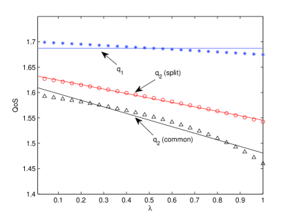
Figure 4: QoS function (with a unit of “bit/sec”) and approximation. The actual and approximated QoS functions are plotted in markers and solid lines, respectively. Approximated QoS functions: $q_{1}=1.687$, $q_{2}=g(\lambda_{2})=1.633-0.088\lambda_{2}$ (split), $q_{2}=g(\lambda_{2})=1.611-0.129\lambda_{2}$ (common).

VII Numerical Results

In this section, we provide numerical results to complement the analysis. For simplicity, we focus on two spectrum sharing schemes, namely, “split” and ‘’common”, which are available for the entrant. Mathematically, the set of available options for the entrant can be denoted by $\{\mathcal{T}_{0}=``\text{Not Enter''},\mathcal{T}_{1}=\text{``Split''},\mathcal{T}_{2}=\text{``Common''}\}$. Since we mainly focus on the entry and technology selection for the entrant, we assume as an example that the incumbent uses the “split” spectrum sharing scheme for its femtocells and macrocells. Note that we can carry out a similar analysis while assuming that the incumbent operates under the “common” spectrum sharing scheme, although the specific results of entry and technology selection for the entrant may be different. We also assume that the incumbent has three times the bandwidth as the entrant, which reflects the fact that the incumbent has more resources than the entrant, and that the users’ valuations of QoS are uniformly distributed in $[0,1]$, i.e., $f(\alpha)=1$ for $\alpha\in[0,1]$.

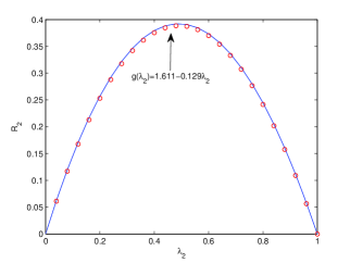
(a) Revenue versus the market share with no incumbent. The revenues based on the actual and approximated QoS functions are plotted in circles and solid line, respectively.

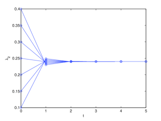
(b) Convergence of the user subscription dynamics with no incumbent. $p_{2}=1.2$ and $q_{2}=g(\lambda_{2})=1.633-0.088\lambda_{2}$ (split).

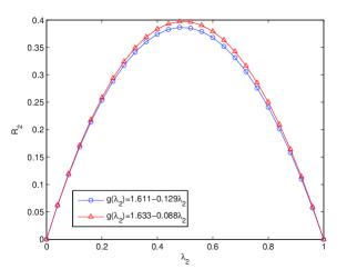
(c) Revenue versus the market share with no incumbent. Circle: common; triangle: split.

Figure 5: Market with no incumbent.

Although our analysis applies to any QoS metric and QoS function satisfying Assumption 1, we shall explicitly consider “average (normalized) throughput”, which has a unit of bit/sec and measures the average transmission rate offered by the NSPs. In a femtocell market, if a user subscribes to either of the two NSPs, it can use femtocell at home and macrocell base stations while staying outdoors. Hence, to derive the average throughput, both the users’ outdoor and indoor accesses need to be considered [2] and the average throughput can be expressed as

$$\begin{split}\mathbb{E}(T_{f})=(1-f_{o})\cdot\mathbb{E}(T_{b})+f_{o}\cdot\mathbb{E}(T_{m}),\end{split}$$ (41)

where $f_{o}$ the fraction of time that users spend outdoors, $T_{b}$ is the throughput obtained by a user from his broadband connection via the femtocell, and $T_{m}$ is the throughput obtained via macrocells. By considering the users’ time-varying positions, transmitted data sizes, and network congestions, the authors in [2] derived an explicit expression of (41) which, due to its complexity, is not shown here. In Table I, we show the network parameters, the meaning of which can be found in [2]. We compute the NSPs’ QoS functions based on (41) derived in [2] and plot them in Fig. 4. Using minimum mean square error fitting, we approximate the QoS provided by NSP $\mathcal{S}_{1}$ using a constant and the QoS provided by NSP $\mathcal{S}_{2}$ using an affine function (i.e., linearly-degrading QoS). The approximated QoS functions are shown as solid lines in Fig. 4. We see from Fig. 4 that although the QoS function of NSP $\mathcal{S}_{1}$ is also decreasing in the number of subscribers, its slope is much less than that of NSP $\mathcal{S}_{2}$’s QoS function and approximating it using a constant still stays close to the actual QoS (within $2\%$). It is also observed from Fig. 4 that the QoS provided by NSP $\mathcal{S}_{2}$ satisfies the property of non-increasing in the number of subscribers. While approximating the QoS using an affine function when NSP $\mathcal{S}_{2}$ uses the “split” spectrum sharing scheme is fairly accurate, the affine approximation is not close to the actual QoS if the “common” spectrum sharing scheme is used. Nevertheless, it can be seen from Fig. 5(a) that the revenue obtained for the (approximated) linearly-degrading QoS function is very close to that obtained for the actual QoS function (within $1\%$). Then, by using the marginal user principle, the optimal prices obtained based on the approximated linearly-degrading and actual QoS functions are $0.837$ and $0.839$, respectively, which are very close to each other (within $1\%$). Thus, approximating the QoS function using an affine function is sufficiently accurate for the purpose of maximizing the revenue, and our previous analysis based on linearly-degrading QoS functions can be applied without losing much accuracy.

VII-A With no incumbent

We first consider a market with no incumbent. Fig. 5(b) illustrates the convergence of the user subscription dynamics for a particular price $p_{2}=1.2$, when the entrant uses the split spectrum sharing technology. Note that given any price $p_{2}\geq 0$, convergence will always be obtained, since the QoS function satisfies the sufficient condition for convergence given in Theorem 1. Note that convergence can also be observed if the entrant uses the common spectrum sharing technology, which is not shown in the paper for brevity. Fig. 5(c) verifies Proposition 2 that the optimal market share maximizing the revenue of NSP $\mathcal{S}_{2}$ is upper bounded by $1/2$. We also observe from Fig. 5(c) that the split spectrum sharing technology can yield a higher revenue for NSP $\mathcal{S}_{2}$, since it provides a higher QoS, compared to the common spectrum sharing technology. Nevertheless, to select the technology that maximizes the entrant’s long-term profit, it also needs to take into account the cost associated with the employed technology (such as developing and implementing spectrum sharing protocol stacks, build base stations that complies with employed technology, etc.). We illustrate in the upper plot of Fig. 6 the technology selection made by the entrant for different costs $k_{1}$ and $k_{2}$. It shows that, even though the split spectrum sharing technology (“split”) offers a higher QoS than the common spectrum sharing technology (“common”) at any number of subscribers, the entrant may still select the “common” technology if the associated cost is sufficiently lower than that associated with the “split” technology. This result quantifies the condition under which the entrant should select “split” or “common”, and serves as a quantitative guidance for the entrant to choose a spectrum sharing technology and maximize its profit.

Figure 6: Technology selection for different costs. Top: with no incumbent; bottom: with one incumbent.

VII-B With one incumbent

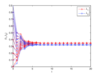
(a) Convergence of market shares under the best-response dynamics.

(b) Convergence of prices under the best-response dynamics.

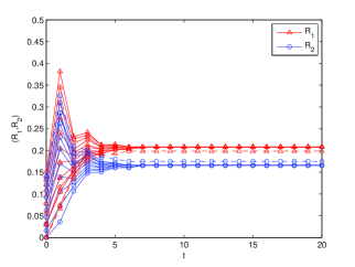
(c) Convergence of revenues under the best-response dynamics.

Figure 7: Market with one incumbent. Dashed and solid lines represent that the entrant uses the split and common spectrum sharing technologies, respectively.

Now, we provide some numerical results regarding the market share competition game. The QoS functions we use in the numerical results are approximate affine functions, rather than the actual QoS functions. Note, however, that we can obtain almost the same results if we use the actual QoS functions, since the affine approximation is sufficiently accurate for analyzing the revenue. The convergence of the considered user subscription dynamics is similar with that in the market with no incumbent, and hence it is omitted due to the space limitations. Starting from different initial points, Figs. 7(a), 7(b), and 7(c) show the convergence of market shares, prices, and revenues, respectively, when both NSPs $\mathcal{S}_{1}$ and $\mathcal{S}_{2}$ update their market shares by choosing their best responses to the market share of the other NSP in the previous period. Since the considered QoS functions satisfy the conditions in Corollary 4, the Cournot competition game with the strategy space $[0,1/2]$ has a unique NE, as verified in Fig. 7(a). Moreover, Fig. 7(a) is consistent with Lemma 1 as the best-response market shares of both NSPs do not exceed 1/2. It can also be observed from Figs. 7(a) and 7(c) that if NSP $\mathcal{S}_{2}$ uses the common spectrum sharing technology that provides a lower QoS (shown in solid lines) compared to that provided by the split spectrum sharing technology (shown in dashed lines), it obtains a smaller revenue, while NSP $\mathcal{S}_{1}$ obtains a higher revenue. This is because when NSP $\mathcal{S}_{2}$ has a lower QoS, it tries to maintain its market share by lowering its price to compensate for the lower QoS, as can be seen from Fig. 7(b). By comparing the entrant’s technology selection in a market with no and one incumbent (shown in Fig. 6), we notice that competition from the incumbent sets a barrier for the entrant to enter the market. That is, the presence of an incumbent lowers the cost threshold under which the entrant earns positive profit from entering the market. Moreover, our analysis provides the entrant with a quantitative guideline as to whether to enter a communications market and which technology to select such that it can maximize its long-term profit.

VIII Conclusion

Focusing on a femtocell market, we studied in this paper the problem of long-term entry and spectrum sharing scheme decision for an entrant. To address the long-term decision, we also studied two related problems: the entrant’s medium-term pricing decisions and the users’ short-term subscription decisions. We considered two scenarios, one with no incumbent and the other with one incumbent. In each scenario, we constructed the user subscription dynamics based on static learning, and showed that there exists a unique equilibrium point of the user subscription dynamics at which the number of subscribers does not change. We provided a sufficient condition on the entrant’s QoS function that ensures the global convergence of the user subscription dynamics. We also examined the revenue maximization problem by the NSPs. With no incumbent in the market, we derived upper and lower bounds on the optimal price and the resulting market share that maximize the entrant’ revenue, for a non-increasing PDF of the users’ valuations of QoS. With one incumbent in the market, we studied competition between the two NSPs, primarily focusing on market share competition. We modeled the NSPs as strategic players in a non-cooperative game where each NSP aims to maximize its own revenue by choosing its market share. We obtained a sufficient condition that ensures the existence of at least one NE of the game. Finally, we formalized the problem of entry and spectrum sharing scheme selection for the entrant and provided numerical results to complete our analysis. Our analysis provides the entrant with a quantitative guideline as to whether to enter a communications market and which technology to select such that it can maximize its long-term profit. Future research directions include, but are not limited to: (1) multiple incumbents and/or entrants in the market; (2) general QoS functions for the incumbents; and (3) social welfare maximization.

Appendix A Proof of Proposition 1

To facilitate the proof, we first define $\tilde{h}_{m}(\lambda_{2})=h_{m}(\lambda_{2})-\lambda_{2}$ for $\lambda_{2}\in[0,1]$, where $h_{m}(\cdot)$ is defined in (3). By Definition 1, $\lambda_{2}^{*}$ is an equilibrium point if and only if it is a root of $\tilde{h}_{m}(\cdot)$. Hence, it suffices to show that $\tilde{h}_{m}(\cdot)$ has a unique root on its domain.

Suppose $p_{2}=0$. Then $h_{m}(\lambda_{2})=1$ for all $\lambda_{2}\in[0,1]$. Thus, $\tilde{h}_{m}(1)=0$ while $\tilde{h}_{m}(\lambda_{2})>0$ for all $\lambda_{2}\in[0,1)$. This implies that $\lambda_{2}=1$ is the unique root of $\tilde{h}_{m}(\cdot)$.

Suppose $0<p_{2}\leq\beta g(1)$. By the fundamental theorem of calculus, $F(\cdot)$ is differentiable on $(0,\beta)$ with $F^{\prime}(\cdot)=f(\cdot)$. By applying the chain rule, we have

$$\frac{d{h}_{m}(\lambda_{2})}{d\lambda_{2}}=f\left(\frac{p_{2}}{g(\lambda_{2})}\right)\frac{g^{\prime}(\lambda_{2})p_{2}}{[g(\lambda_{2})]^{2}}$$ (42)

for all $\lambda_{2}\in(0,1)$. By Assumption 1, $g^{\prime}(\cdot)\leq 0$ on $(0,1)$, and thus $d{h}_{m}(\cdot)/d\lambda_{2}\leq 0$ on $(0,1)$. Since $d\tilde{h}_{m}(\cdot)/d\lambda_{2}=d{h}_{m}(\cdot)/d\lambda_{2}-1$, $\tilde{h}_{m}(\cdot)$ is strictly decreasing on $[0,1]$. Next, we note that $\tilde{h}_{m}(0)=h_{m}(0)=1-F(p_{2}/g(0))\geq 0$ and $\tilde{h}_{m}(1)=-F(p_{2}/g(1))<0$. Since $\tilde{h}_{m}(\cdot)$ is continuous on $[0,1]$, we obtain a unique root of $\tilde{h}_{m}(\cdot)$ on $[0,1]$ by applying the intermediate value theorem.

Suppose $\beta g(1)<p_{2}<\beta g(0)$. Let $\bar{\lambda}_{2}=\min\{\lambda_{2}\in[0,1]|\beta g(\lambda_{2})\leq p_{2}\}$. Note that $\bar{\lambda}_{2}\in(0,1)$. Also, $h_{m}(\lambda_{2})=0$ for all $\lambda_{2}\geq\bar{\lambda}_{2}$, and thus $\tilde{h}_{m}(\lambda_{2})=-\lambda_{2}<0$ for all $\lambda_{2}\geq\bar{\lambda}_{2}$. Hence, if a root of $\tilde{h}_{m}(\cdot)$ exists, it must be in $[0,\bar{\lambda}_{2})$. By applying a similar argument as above to the interval $[0,\bar{\lambda}_{2}]$, we can show that $\tilde{h}_{m}(\cdot)$ has a unique root on $[0,\bar{\lambda}_{2}]$.

Suppose $p_{2}\geq\beta g(0)$. Then $h_{m}(\lambda_{2})=0$ for all $\lambda_{2}\in[0,1]$. Thus, $\tilde{h}_{m}(0)=0$ while $\tilde{h}_{m}(\lambda_{2})<0$ for all $\lambda_{2}\in(0,1]$. This implies that $\lambda_{2}=0$ is the unique root of $\tilde{h}_{m}(\cdot)$. $\blacksquare$

Appendix B Proof of Theorem 1

We prove the convergence of the user subscription dynamics in the market with no incumbent based on the contraction mapping theorem.

Definition 4 [24]: A mapping $\mathbf{T}:\,\mathcal{X}\to\mathcal{X}$, where $\mathcal{X}$ is a closed subset of $\mathbb{R}^{n}$, is called a contraction if there is a real number $\kappa\in[0,1)$ such that

$$\|\mathbf{T}(x_{1})-\mathbf{T}(x_{2})\|\leq\kappa\|x_{1}-x_{2}\|,\;\;\;\forall\;x_{1},x_{2}\in\mathcal{X},$$ (43)

where $\|\cdot\|$ is some norm defined on $\mathcal{X}$.

Proposition 1.1 in Chapter 3 of [24] shows an important property of a contraction mapping $\mathbf{T}$ that the update sequence generated by $x^{t+1}=\mathbf{T}(x^{t})$, $t=0,1,2,\ldots$, converges to a fixed point $x^{*}$ satisfying $\mathbf{T}(x^{*})=x^{*}$ starting from any initial value $x^{0}\in\mathcal{X}$. To prove Theorem 1, we shall show that the function $h_{m}(\cdot)$, defined in (3), is a contraction mapping on $[0,1]$ with respect to the absolute value norm if the condition (6) is satisfied.

Suppose $p_{2}=0$. Then $h_{m}(\lambda_{2})=1$ for all $\lambda_{2}\in[0,1]$, and thus $h_{m}(\cdot)$ is a contraction with $\kappa=0$.

Suppose $p_{2}>0$. Let $\lambda_{2,a}$ and $\lambda_{2,b}$ be two different real numbers arbitrarily chosen from the interval $[0,1]$, and suppose without loss of generality that $\lambda_{2,a}>\lambda_{2,b}$. We will show that

$$|h_{m}(\lambda_{2,a})-h_{m}(\lambda_{2,b})|\leq\kappa_{m}|\lambda_{2,a}-\lambda_{2,b}|,$$ (44)

where $\kappa_{m}=K\cdot\max_{\lambda_{2}\in[0,1]}\{-g^{\prime}(\lambda_{2})/g(\lambda_{2})\}$. Then the condition (6) implies that $\kappa_{m}\in[0,1)$, establishing that $h_{m}(\cdot)$ is a contraction. Since $0<p_{2}/g(\lambda_{2,b})\leq p_{2}/g(\lambda_{2,a})$, we can consider three cases.

Case 1 ($p_{2}/g(\lambda_{2,a}),p_{2}/g(\lambda_{2,b})<\beta$): Note that $h_{m}$ is continuous on $[0,1]$ and differentiable on $(\lambda_{2,b},\lambda_{2,a})$. Hence, by the mean value theorem, there exists $\lambda_{2,c}\in(\lambda_{2,b},\lambda_{2,a})$ such that

$$h^{\prime}_{m}(\lambda_{2,c})=\frac{h_{m}(\lambda_{2,a})-h_{m}(\lambda_{2,b})}{\lambda_{2,a}-\lambda_{2,b}}.$$ (45)

Then we obtain

$$|h_{m}(\lambda_{2,a})-h_{m}(\lambda_{2,b})|$$ (46)

$$= \left|f\left(\frac{p_{2}}{g(\lambda_{2,c})}\right)\frac{p_{2}}{g(\lambda_{2,c})}\frac{g^{\prime}(\lambda_{2,c})}{g(\lambda_{2,c})}\right||\lambda_{2,a}-\lambda_{2,b}|$$ (47)

$$\leq \kappa_{m}|\lambda_{2,a}-\lambda_{2,b}|.$$ (48)

Case 2 ($p_{2}/g(\lambda_{2,b})<\beta\leq p_{2}/g(\lambda_{2,a})$): Let $\bar{\lambda}_{2}=\min\{\lambda_{2}\in[0,1]|\ \beta g(\lambda_{2})\leq p_{2}\}$. Note that $\lambda_{2,b}<\bar{\lambda}_{2}\leq\lambda_{2,a}$. Applying the mean value theorem to $h_{m}(\cdot)$ on the interval $[\lambda_{2,b},\bar{\lambda}_{2}]$ yields

$$|h_{m}(\bar{\lambda}_{2})-h_{m}(\lambda_{2,b})|\leq\kappa_{m}|\bar{\lambda}_{2}-\lambda_{2,b}|.$$ (49)

Since $h_{m}(\bar{\lambda}_{2})=h_{m}(\lambda_{2,a})=0$ and $\kappa_{m}\geq 0$, we obtain

$$\begin{split}|h_{m}(\lambda_{2,a})-h_{m}(\lambda_{2,b})|&=|h_{m}(\bar{\lambda}_{2})-h_{m}(\lambda_{2,b})|\\ &\leq\kappa_{m}|\bar{\lambda}_{2}-\lambda_{2,b}|\\ &\leq\kappa_{m}|\lambda_{2,a}-\lambda_{2,b}|.\end{split}$$ (50)

Case 3 ($p_{2}/g(\lambda_{2,a}),p_{2}/g(\lambda_{2,b})\geq\beta$): In this case, $h_{m}(\lambda_{2,a})=h_{m}(\lambda_{2,b})=0$, and (44) is trivially satisfied. $\blacksquare$

Appendix C Proof of Proposition 2

To prove Proposition 2, we shall show that a solution $\lambda_{2}^{**}$ of $\max_{\lambda_{2}\in[0,1]}F^{-1}(1-\lambda_{2})g(\lambda_{2})\lambda_{2}$ satisfies $0<\lambda_{2}^{**}\leq 1/2$. Then $F^{-1}(1/2)\leq\alpha^{*}<\beta$ follows from the relationship $\alpha^{*}=F^{-1}(1-\lambda_{2}^{**})$ and $F^{-1}(1/2)g(1/2)\leq p_{2}^{*}<\beta g(0)$ from $p_{2}^{*}=\alpha^{*}g(1-F(\alpha^{*}))$. Note first that $\lambda_{2}^{**}$ cannot be zero because the maximum revenue is positive. Thus, it remains to show $\lambda_{2}^{**}\leq 1/2$.

Let $z(\lambda_{2})=F^{-1}(1-\lambda_{2})$ for $\lambda_{2}\in[0,1]$. Then $z(\cdot)$ is differentiable on $(0,1)$ with the derivative $z^{\prime}(\lambda_{2})=dz(\lambda_{2})/d\lambda_{2}=-1/f(z(\lambda_{2}))$. Note that $z^{\prime}(\lambda_{2})<0$ for all $\lambda_{2}\in(0,1)$, which implies that $z(\cdot)$ is strictly decreasing on $[0,1]$. Also, since $f(\cdot)$ is non-increasing on $[0,\beta]$, $z^{\prime}(\cdot)$ is non-decreasing on $(0,1)$. The revenue of NSP $\mathcal{S}_{2}$ can be expressed as a function of $\lambda_{2}$, $R_{2}(\lambda_{2})=\lambda_{2}g(\lambda_{2})z(\lambda_{2})$. Since $R_{2}(\cdot)$ is differentiable and $\lambda_{2}^{**}\in(0,1)$ ($\lambda_{2}=1$ yields zero revenue and thus cannot be optimal), the first-order necessary condition implies that

$$\begin{split}\frac{dR_{2}(\lambda_{2}^{**})}{d\lambda_{2}}=&\left[z(\lambda_{2}^{**})+\lambda_{2}^{**}z^{\prime}(\lambda_{2}^{**})\right]g(\lambda_{2}^{**})\\ &+\lambda_{2}^{**}z(\lambda_{2}^{**})g^{\prime}(\lambda_{2}^{**})=0.\end{split}$$ (51)

Note that $\lambda_{2}^{**}z(\lambda_{2}^{**})g^{\prime}(\lambda_{2}^{**})\leq 0$. Thus, $z(\lambda_{2}^{**})+\lambda_{2}^{**}z^{\prime}(\lambda_{2}^{**})\geq 0$. By the mean value theorem, there exists $\hat{\lambda}_{2}\in(\lambda_{2}^{**},1)$ such that $z(\lambda_{2}^{**})=z(\lambda_{2}^{**})-z(1)=z^{\prime}(\hat{\lambda}_{2})(\lambda_{2}^{**}-1)$. Then we have

$$0 \leq z(\lambda_{2}^{**})+\lambda_{2}^{**}z^{\prime}(\lambda_{2}^{**})$$ (52)

$$=z^{\prime}(\hat{\lambda}_{2})(\lambda_{2}^{**}-1)+\lambda_{2}^{**}z^{\prime}(\lambda_{2}^{**})$$ (53)

$$\leq z^{\prime}(\lambda_{2}^{**})(\lambda_{2}^{**}-1)+\lambda_{2}^{**}z^{\prime}(\lambda_{2}^{**})$$ (54)

$$=z^{\prime}(\lambda_{2}^{**})(2\lambda_{2}^{**}-1),$$ (55)

which implies $\lambda_{2}^{**}\leq 1/2$. $\blacksquare$

Appendix D Proof of Proposition 3

We consider two cases depending on the relative values of $p_{1}/q_{1}$ and $p_{2}/g(0)$.

Case 1 ($p_{1}/q_{1}\leq p_{2}/g(0)$): Let $\lambda_{1}^{*}=1-F(p_{1}/q_{1})$ and $\lambda_{2}^{*}=0$. Since $p_{1}/q_{1}\leq p_{2}/g(\lambda_{2}^{*})$, $h_{d,1}(\lambda_{1}^{*},\lambda_{2}^{*})$ and $h_{d,2}(\lambda_{1}^{*},\lambda_{2}^{*})$ are determined by (22) and (23), respectively. Thus, $h_{d,1}(\lambda_{1}^{*},\lambda_{2}^{*})=\lambda_{1}^{*}$ and $h_{d,2}(\lambda_{1}^{*},\lambda_{2}^{*})=\lambda_{2}^{*}$, and by Definition 3, $(\lambda_{1}^{*},\lambda_{2}^{*})$ is an equilibrium point. By the non-increasing property of $g(\cdot)$, we have $p_{1}/q_{1}\leq p_{2}/g(0)\leq p_{2}/g(\lambda_{2})$ for all $\lambda_{2}\in[0,1]$. Thus, the user subscription dynamics in Case 1 is described by (22) and (23). This establishes the uniqueness of the equilibrium point $(\lambda_{1}^{*},\lambda_{2}^{*})$, because $h_{d,i}(\cdot)$ cannot take a value different from $\lambda_{i}^{*}$, for $i=1,2$.

Case 2 ($p_{1}/q_{1}>p_{2}/g(0)$): Since $h_{d,2}(\cdot)$ is independent of $\lambda_{1}$, we can express $h_{d,2}(\cdot)$ as a function of $\lambda_{2}$ only:

$$h_{d,2}(\lambda_{2})=\left\{\begin{array}[]{ll}F\left(\frac{p_{1}-p_{2}}{q_{1}-g(\lambda_{2})}\right)-F\left(\frac{p_{2}}{g(\lambda_{2})}\right)&\text{if }\frac{p_{1}}{q_{1}}>\frac{p_{2}}{g(\lambda_{2})},\\ 0&\;\;\;\;\;\;\text{otherwise}.\end{array}\right.$$ (58)

Note that $h_{d,2}(\cdot)$ is continuous and non-increasing on $[0,1]$. Let $\tilde{h}_{d,2}(\lambda_{2})=h_{d,2}(\lambda_{2})-\lambda_{2}$ for all $\lambda_{2}\in[0,1]$. Then $\tilde{h}_{d,2}(\cdot)$ is continuous and strictly decreasing on $[0,1]$. Since $p_{1}/q_{1}>p_{2}/g(0)$, we have

$$\tilde{h}_{d,2}(0)=h_{d,2}(0)-0=F\left(\frac{p_{1}-p_{2}}{q_{1}-g(0)}\right)-F\left(\frac{p_{2}}{g(0)}\right)>0.$$ (59)

Also,

$$\tilde{h}_{d,2}(1) =h_{d,2}(1)-1$$

$$=\left\{\begin{array}[]{ll}F\left(\frac{p_{1}-p_{2}}{q_{1}-g(1)}\right)-F\left(\frac{p_{2}}{g(1)}\right)-1&\text{if }\frac{p_{1}}{q_{1}}>\frac{p_{2}}{g(1)},\\ -1&\;\;\;\;\text{otherwise}.\end{array}\right.$$ (62)

Hence, $\tilde{h}_{d,2}(1)\leq 0$, and there exists unique $\lambda_{2}^{*}\in(0,1]$ such that $h_{d,2}(\lambda_{2}^{*})=\lambda_{2}^{*}$. Suppose that $p_{1}/q_{1}\leq p_{2}/g(\lambda_{2}^{*})$. Then $\lambda_{2}^{*}=h_{d,2}(\lambda_{2}^{*})=0$, which is a contradiction. Hence, $\lambda_{2}^{*}$ must satisfy $p_{1}/q_{1}>p_{2}/g(\lambda_{2}^{*})$. Let $\lambda_{1}^{*}=F\left((p_{1}-p_{2})/(q_{1}-g(\lambda_{2}^{*}))\right)$. Then it is easy to verify that $(\lambda_{1}^{*},\lambda_{2}^{*})$ is an equilibrium point. This equilibrium point is unique because $\lambda_{2}^{*}$ is the unique fixed point of $h_{d,2}(\cdot)$. $\blacksquare$

Appendix E Proof of Theorem 2

For notational convenience, we use $h_{d,1}(\lambda_{2})$ and $h_{d,2}(\lambda_{2})$ instead of $h_{d,1}(\lambda_{1},\lambda_{2})$ and $h_{d,2}(\lambda_{1},\lambda_{2})$, respectively, since they are independent of $\lambda_{1}$. Note that $h_{d,1}(\cdot)$ is a non-decreasing function of $\lambda_{2}$ while $h_{d,2}(\cdot)$ is a non-increasing function of $\lambda_{2}$. Define a mapping $\mathbf{h}_{d}:\Lambda\to\Lambda$ by

$$\mathbf{h}_{d}(\lambda_{1},\lambda_{2})=\left(h_{d,1}(\lambda_{2}),h_{d,2}(\lambda_{2})\right).$$ (63)

To prove Theorem 2, we shall show that the mapping $\mathbf{h}_{d}(\cdot)$ is a contraction on $\Lambda$ with respect to the maximum norm [24] if the condition (26) is satisfied.

Let $\lambda_{a}=(\lambda_{1,a},\lambda_{2,a})$ and $\lambda_{b}=(\lambda_{1,b},\lambda_{2,b})$ be two different vectors arbitrarily chosen from the set $\Lambda$, and suppose without loss of generality that $\lambda_{2,a}\geq\lambda_{2,b}$. We will show that

$$\|\mathbf{h}_{d}(\lambda_{1,a},\lambda_{2,a})-\mathbf{h}_{d}(\lambda_{1,b},\lambda_{2,b})\|_{\infty}\leq\kappa_{d}\left\|\lambda_{a}-\lambda_{b}\right\|_{\infty},$$ (64)

where $\kappa_{d}=K\cdot\max_{\lambda_{2}\in[0,1]}\left\{[-g^{\prime}(\lambda_{2})/g(\lambda_{2})]\cdot[q_{1}/(q_{1}-g(\lambda_{2}))]\right\}$. Then the condition (26) implies that $\kappa_{d}\in[0,1)$, establishing that $\mathbf{h}_{d}(\cdot)$ is a contraction. Since $p_{2}/g(\lambda_{2,b})\leq p_{2}/g(\lambda_{2,a})$, we can consider three cases.

Case 1 ($p_{2}/g(\lambda_{2,a}),p_{2}/g(\lambda_{2,b})<p_{1}/q_{1}$): In this case, both $\mathbf{h}_{d}(\lambda_{1,a},\lambda_{2,a})$ and $\mathbf{h}_{d}(\lambda_{1,b},\lambda_{2,b})$ are determined by (20) and (21). Hence,

$$\|\mathbf{h}_{d}(\lambda_{1,a},\lambda_{2,a})-\mathbf{h}_{d}(\lambda_{1,b},\lambda_{2,b})\|_{\infty}$$ (65)

$$= \max_{i=1,2}\{\left|h_{d,i}(\lambda_{2,a})-h_{d,i}(\lambda_{2,b})\right|\}$$ (67)

$$= \max\left\{F\left(\frac{p_{1}-p_{2}}{q_{1}-g(\lambda_{2,b})}\right)-F\left(\frac{p_{1}-p_{2}}{q_{1}-g(\lambda_{2,a})}\right)\right.,$$

$$\;\;\;\;\;\;\;\;\;F\left(\frac{p_{1}-p_{2}}{q_{1}-g(\lambda_{2,b})}\right)-F\left(\frac{p_{1}-p_{2}}{q_{1}-g(\lambda_{2,a})}\right)$$

$$\left.\;\;\;\;\;\;\;\;\;+F\left(\frac{p_{2}}{g(\lambda_{2,a})}\right)-F\left(\frac{p_{2}}{g(\lambda_{2,b})}\right)\right\}$$

$$= h_{d,2}(\lambda_{2,b})-h_{d,2}(\lambda_{2,a})\,.$$ (68)

Note that (64) is trivially satisfied if $\lambda_{2,a}=\lambda_{2,b}$. Thus, we assume that $\lambda_{2,a}>\lambda_{2,b}$. We first consider the case where $0<p_{2}/g(\lambda_{2,b})\leq p_{2}/g(\lambda_{2,a})<\beta$ and $0<(p_{1}-p_{2})/(q_{1}-g(\lambda_{2,a}))\leq(p_{1}-p_{2})/(q_{1}-g(\lambda_{2,b}))<\beta$ so that $h_{d,2}(\cdot)$ is differentiable on $(\lambda_{2,b},\lambda_{2,a})$. Then by the mean value theorem, there exists $\lambda_{2,c}\in(\lambda_{2,b},\lambda_{2,a})$ such that $h_{d,2}(\lambda_{2,b})-h_{d,2}(\lambda_{2,a})=h^{\prime}_{d,2}(\lambda_{2,c})(\lambda_{2,b}-\lambda_{2,a})$. Therefore,

$$\left\|\mathbf{h}_{d}(\lambda_{1,a},\lambda_{2,a})-\mathbf{h}_{d}(\lambda_{1,b},\lambda_{2,b})\right\|_{\infty}$$ (69)

$$= \Bigg{\{}-f\left(\frac{p_{1}-p_{2}}{q_{1}-g(\lambda_{2,c})}\right)\frac{\left(p_{1}-p_{2}\right)g^{\prime}(\lambda_{2,c})}{\left[q_{1}-g(\lambda_{2,c})\right]^{2}}$$ (70)

$$-f\left(\frac{p_{2}}{g(\lambda_{2,c})}\right)\frac{p_{2}g^{\prime}(\lambda_{2,c})}{(g(\lambda_{2,c}))^{2}}\Bigg{\}}\left|\lambda_{2,a}-\lambda_{2,b}\right|$$ (71)

$$\leq \ K\left[-\frac{g^{\prime}(\lambda_{2,c})}{q_{1}-g(\lambda_{2,c})}-\frac{g^{\prime}(\lambda_{2,c})}{g(\lambda_{2,c})}\right]\left|\lambda_{2,a}-\lambda_{2,b}\right|$$ (72)

$$= \ K\left[-\frac{g^{\prime}(\lambda_{2,c})}{g(\lambda_{2,c})}\cdot\frac{q_{1}}{q_{1}-g(\lambda_{2,c})}\right]\left|\lambda_{2,a}-\lambda_{2,b}\right|$$ (73)

$$\leq \ \kappa_{d}\left\|\lambda_{a}-\lambda_{b}\right\|_{\infty}.$$ (74)

The cases where $0<p_{2}/g(\lambda_{2,b})\leq p_{2}/g(\lambda_{2,a})<\beta$ or $0<(p_{1}-p_{2})/(q_{1}-g(\lambda_{2,a}))\leq(p_{1}-p_{2})/(q_{1}-g(\lambda_{2,b}))<\beta$ does not hold can be covered as in the proof of Theorem 1.

Case 2 ($p_{2}/g(\lambda_{2,b})<p_{1}/q_{1}\leq p_{2}/g(\lambda_{2,a})$): In this case, $\mathbf{h}_{d}(\lambda_{1,a},\lambda_{2,a})$ is determined by (22) and (23), while $\mathbf{h}_{d}(\lambda_{1,b},\lambda_{2,b})$ is determined by (20) and (21). Hence,

$$\|\mathbf{h}_{d}(\lambda_{1,a},\lambda_{2,a})-\mathbf{h}_{d}(\lambda_{1,b},\lambda_{2,b})\|_{\infty}$$ (75)

$$= \max\left\{F\left(\frac{p_{1}-p_{2}}{q_{1}-g(\lambda_{2,b})}\right)-F\left(\frac{p_{1}}{q_{1}}\right),\right.$$ (76)

$$\left.\;\;\;\;\;\;\;\;\;F\left(\frac{p_{1}-p_{2}}{q_{1}-g(\lambda_{2,b})}\right)-F\left(\frac{p_{2}}{g(\lambda_{2,b})}\right)\right\}$$ (77)

$$= F\left(\frac{p_{1}-p_{2}}{q_{1}-g(\lambda_{2,b})}\right)-F\left(\frac{p_{2}}{g(\lambda_{2,b})}\right)$$ (78)

$$= h_{d,2}(\lambda_{2,b})-h_{d,2}(\lambda_{2,a})$$ (79)

Let $\bar{\lambda}_{2}=\min\{\lambda_{2}\in[0,1]|\ g(\lambda_{2})p_{1}/q_{1}\leq p_{2}\}$. Note that $\lambda_{2,b}<\bar{\lambda}_{2}\leq\lambda_{2,a}$. Again, we focus on the case where $0<p_{2}/g(\lambda_{2,b})\leq p_{2}/g(\bar{\lambda}_{2})<\beta$ and $0<(p_{1}-p_{2})/(q_{1}-g(\bar{\lambda}_{2}))\leq(p_{1}-p_{2})/(q_{1}-g(\lambda_{2,b}))<\beta$, while omitting the other cases. Applying the mean value theorem to $h_{d,2}(\cdot)$ on the interval $[\lambda_{2,b},\bar{\lambda}_{2}]$ yields

$$|h_{d,2}(\bar{\lambda}_{2})-h_{d,2}(\lambda_{2,b})|\leq\kappa_{d}|\bar{\lambda}_{2}-\lambda_{2,b}|.$$ (80)

Since $h_{d,2}(\bar{\lambda}_{2})=h_{d,2}(\lambda_{2,a})=0$ and $\kappa_{d}\geq 0$, we obtain

$$\|\mathbf{h}_{d}(\lambda_{1,a},\lambda_{2,a})-\mathbf{h}_{d}(\lambda_{1,b},\lambda_{2,b})\|_{\infty}$$ (81)

$$= |h_{d,2}(\lambda_{2,a})-h_{d,2}(\lambda_{2,b})|$$ (82)

$$= |h_{d,2}(\bar{\lambda}_{2})-h_{d,2}(\lambda_{2,b})|$$ (83)

$$\leq \kappa_{d}|\bar{\lambda}_{2}-\lambda_{2,b}|\leq\kappa_{d}|\lambda_{2,a}-\lambda_{2,b}|$$ (84)

$$\leq \kappa_{d}\left\|\lambda_{a}-\lambda_{b}\right\|_{\infty}.$$ (85)

Case 3 ($p_{2}/g(\lambda_{2,a}),p_{2}/g(\lambda_{2,b})\geq p_{1}/q_{1}$): In this case, both $\mathbf{h}_{d}(\lambda_{1,a},\lambda_{2,a})$ and $\mathbf{h}_{d}(\lambda_{1,b},\lambda_{2,b})$ are determined by (22) and (23). Hence, $\mathbf{h}_{d}(\lambda_{1,a},\lambda_{2,a})=\mathbf{h}_{d}(\lambda_{1,b},\lambda_{2,b})=(1-F(p_{1}/q_{1}),0)$, and (64) is trivially satisfied. $\blacksquare$

Appendix F Proof of Theorem 3

Let $\tilde{\mathcal{G}}^{\prime}_{C}=\left\{\mathcal{S}_{i},R_{i}(\lambda_{1},\lambda_{2}),\lambda_{i}\in[0,1/2]\;|\;i=1,2\right\}$. Since $f(\cdot)$ is non-increasing, the set of NE of $\tilde{\mathcal{G}}_{C}$ is equal to that of $\tilde{\mathcal{G}}^{\prime}_{C}$ by Lemma 1, and thus it suffices to prove the existence of NE of $\tilde{\mathcal{G}}^{\prime}_{C}$. Since $[0,1/2]^{2}\subset\Lambda$, the expression of $R_{i}(\lambda_{1},\lambda_{2})$ in $\tilde{\mathcal{G}}^{\prime}_{C}$ is given by $R_{i}(\lambda_{1},\lambda_{2})=\lambda_{i}p_{i}(\lambda_{1},\lambda_{2})$, for $i=1,2$. Since $f(\cdot)$ is continuously differentiable on $[0,\beta]$, $R_{i}(\cdot)$ is twice continuously differentiable on $[0,1/2]^{2}$. The second-order mixed partial derivatives of $R_{1}(\cdot)$ and $R_{2}(\cdot)$ are given by the negative of the left-hand sides of (36) and (37), respectively. Therefore, (36) and (37) imply that $\frac{\partial^{2}R_{i}(\lambda_{1},\lambda_{2})}{\partial\lambda_{1}\partial\lambda_{2}}\leq 0$, for all $(\lambda_{1},\lambda_{2})\in[0,1/2]^{2}$, for all $i=1,2$. Consider a transformed game of $\tilde{\mathcal{G}}^{\prime}_{C}$,

$$\begin{split}\tilde{\mathcal{G}}^{\prime\prime}_{C}=&\left\{\mathcal{S}_{1},\mathcal{S}_{2},\tilde{R}_{1}(\mu_{1},\lambda_{2}),\tilde{R}_{2}(\mu_{1},\lambda_{2}),\right.\\ &\;\;\;\;\;\mu_{1}\in[-1/2,0],\lambda_{2}\in[0,1/2]\Big{\}},\end{split}$$ (86)

where $\tilde{R}_{i}(\mu_{1},\lambda_{2})=R_{i}(-\mu_{1},\lambda_{2})$ for all $(\mu_{1},\lambda_{2})\in[-1/2,0]\times[0,1/2]$, for $i=1,2$. Since $\tilde{R}_{1}(\cdot)$ and $\tilde{R}_{2}(\cdot)$ are continuous in both arguments and have increasing differences in $(\mu_{1},\lambda_{2})$ and in $(\lambda_{2},\mu_{1})$, respectively, $\tilde{\mathcal{G}}^{\prime\prime}_{C}$ is a supermodular game [26]. Therefore, $\tilde{\mathcal{G}}^{\prime\prime}_{C}$ has at least one pure NE, and $\tilde{\mathcal{G}}^{\prime}_{C}$ also has a corresponding NE. $\blacksquare$

References

- [1] J. D. Hobby and H. Claussen, “Deployment options for femtocells and their impact on existing macrocellular networks,” Bell Labs Tech. Jnl., vol. 13, no. 4, pp. 145 C160, 2009.
- [2] N. Shetty, S. Parekh, and J. Walrand, “Economics of femtocells,” IEEE Globecom, Dec. 2009.
- [3] N., Shetty, G. Schwartz, and J. Walrand, “Internet QoS and regulations,” IEEE/ACM Trans. Networking, vol. 18, no. 6, pp. 1725-1737, Dec. 2010.
- [4] Y. Jin, S. Sen, R. Guerin, K. Hosanagar, and Z.-L. Zhang, “Dynamics of competition between incumbent and emerging network technologies,” NetEcon, Seattle, WA, USA, August 22, 2008.
- [5] J. Musacchio and D. Kim, “Network platform competition in a two-sided market: implications to the net neutrality issue,” TPRC: Conference on Communication, Information, and Internet Policy, Sep. 2009.
- [6] L. He and J. Walrand, “Pricing and revenue sharing strategies for Internet service providers,” IEEE J. Sel. Areas Commun., vol. 24, no. 5, pp. 942-951, May 2006.
- [7] P. Hande, M. Chiang, A. R. Calderbank, and S. Rangan, “Network pricing and rate allocation with content provider participation,” IEEE Infocom, Apr. 2009.
- [8] M. Manshaei, J. Freudiger, M. Felegyhazi, P. Marbach, and J. P. Hubaux, “On wireless social community networks,” IEEE Infocom, Apr. 2008.
- [9] D. Acemoglu and A. Ozdaglar, “Competition and efficiency in congested markets,” Mathematics of Operations Research, vol. 32, no. 1, pp. 1-31, 2007.
- [10] R. Johari, G.Y. Weintraub, and B. Van Roy, “Investment and market structure in industries with congestion,” Operations Research, vol. 58 no. 5, pp. 1303-1317, 2010.
- [11] O. Candogan, K. Bimpikis, and A. Ozdaglar, “Optimal pricing in networks with externalities,” available at http://arxiv.org/abs/1101.5617.
- [12] L. Jiang, S. Parekh, and J. Walrand, “Time-dependent network pricing and bandwidth trading,” IEEE Intl. Workshop Bandwidth on Demand, 2008.
- [13] Z. Zhang and C. Douligeris, “Convergence of synchronous and asynchronous greedy algorithm in a multiclass telecommunications environment,” IEEE Tran. Commun., vol. 40, pp. 1277-1281, 1992.
- [14] A. Zemlianov and G. de Veciana, “Cooperation and decision making in wireless multiprovider setting,” IEEE Infocom, Mar. 2005.
- [15] C. K. Chau, Q. Wang, and D. M. Chiu, “On the viability of Paris metro pricing for communication and service networks,” IEEE Infocom, Mar. 2010.
- [16] Z. Kun, D. Niyato, and P. Wang, “Optimal bandwidth allocation with dynamic service selection in heterogeneous wireless networks,” to appear in IEEE Globecom, Dec. 2010.
- [17] S. Shakkottai, R. Srikant, A. Ozdaglar and D. Acemoglu, “The price of simplicity,” IEEE J. Sel. Areas in Commun., pp. 1269-1276, vol. 26, no. 7, Sep. 2008.
- [18] D. Acemoglu, A. Ozdaglar, and R. Srikant, “The marginal user principle for resource allocation in wireless networks,” IEEE CDC, 2004.
- [19] S. Ren and M. van der Schaar “Data demand dynamics in wireless communications markets,” IEEE Trans. Signal Process., vol. 60, no. 4, pp. 1986-2000, Apr. 2011.
- [20] J. Lee, J. Yoon, M. Nguyen, and H. Lee, “Traffic pattern based resource hopping schemes of femto base stations,” IEEE CNCC, 2010.
- [21] M. Cheboldaeff, “Interactions between a Mobile Virtual Network Operator and External Networks with Regard to Service Triggering” IEEE Intl. Conf. Networking, 2007.
- [22] S. Haykin, “Cognitive radio: Brain-empowered wireless communications” IEEE J. Sel. Areas Commun., vol. 23, no. 2, pp. 201-220, Feb. 2005.
- [23] G. W. Evans and S. Honkapohja, Learning and Expectations in Macroeconomics Princeton, NJ: Princeton Univ. Press, 2001.
- [24] D. P. Bertsekas and J. N. Tsitsiklis, Parallel and Distributed Computation: Numerical Methods, Belmont, MA: Athena Scientific, 1989.
- [25] M. J. Osborne and A. Rubinstein, A Course in Game Thoeory. Cambridge, MA: MIT Press, 1994.
- [26] D. M. Topkis, Supermodularity and Complementarity. Princeton, NJ: Princeton Univ. Press, 1998.
- [27] J. Tirole, The Theory of Industrial Organization. Cambridge, MA: MIT Press, 1988.