HII Regions, Embedded Protostars, and Starless Cores in Sharpless 2-157

Abstract

We present arcsecond resolution 1.4mm observations of the high mass star forming region, Sharpless 2-157, that reveal the cool dust associated with the first stages of star formation. These data are compared with archival images at optical, infrared, and radio wavelengths, and complemented with new arcsecond resolution mid-infrared data. We identify a dusty young HII region, numerous infrared sources within the cluster envelope, and four starless condensations. Three of the cores lie in a line to the south of the cluster peak, but the most massive one is right at the center and associated with a jumble of bright radio and infrared sources. This presents an interesting juxtaposition of high and low mass star formation within the same cluster which we compare with similar observations of other high mass star forming regions and discuss in the context of cluster formation theory.

1. Introduction

Decades of observations of the closest molecular clouds have revealed much about the formation of isolated low mass stars and the stages of individual core collapse, protostellar birth, disk accretion, and eventual dissipation of the surrounding envelope (Evans et al., 2009; McKee & Ostriker, 2007). Such regions, however, are not the typical birth environments of most stars, as is clear from the statistics of stellar clusters (Lada & Lada, 2003) and as inferred from the number of high mass, ionizing stars in the Galaxy and the expectation from the IMF that they be accompanied by large numbers of lower mass stars (McKee & Williams, 1997). There is also considerable cosmochemical evidence that our Sun formed in a large cluster, in close proximity to a massive star (Dauphas & Chaussidon, 2011; Williams, 2010). A more complete understanding of our origins requires studies of a broader range of stellar birth environments including clusters and high mass star forming regions.

High mass stars, $M_{\ast}\gtrsim 8\,M_{\odot}$, cannot form in exactly the same way that solar mass stars form because spherically symmetric accretion at the thermal sound speed would be turned back by radiation pressure (Wolfire & Cassinelli, 1987). Self-similar turbulence provides a way to extend the low mass paradigm to higher masses by providing enhanced accretion at the turbulent, rather than thermal, speed (McKee & Tan, 2003). Infall onto the star may also slip through radiation bubbles via Rayleigh-Taylor instabilities (Krumholz et al., 2009). Bonnell et al. (1998) proposed the coalescence of low mass stars as a means to bypass the radiation pressure problem but the observed density of young stellar clusters does not appear high enough for this to be viable. The main alternative to the picture of quasistatic collapse of a massive core is the dynamic scenario of competitive accretion of a cluster of stars in a dense clump (Bonnell & Bate, 2006). Here, stars at the center of the cluster potential well grow rapidly to high masses, whereas stars in the outer parts grow more slowly. Detailed, multi-wavelength observations are required to test these different scenarios.

Massive stars evolve much faster than low mass stars, achieving hydrogen fusion while still accreting material from their surroundings. Together with their intrinsic rarity, this means that high mass protostars are few and far between. High resolution observations are therefore required to distinguish them from their clustered surroundings. Their high luminosities, however, make them readily apparent and the ionized (HII) gas that they produce shortly after their birth can be detected at radio wavelengths where Galactic extinction is negligible and is an unambiguous signature of their nature as massive stars.

Here, we present a high resolution, multi-wavelength study of the massive star forming region, Sh2-157. First cataloged by Sharpless (1959) on the basis of its optical nebulosity, this well studied region has an estimated kinematic distance of 2.5 kpc (Fich & Blitz, 1984). The large HII region, Sh2-157A, is powered by a late O star (Chopinet & Lortet-Zuckermann, 1972) but radio observations by Israel et al. (1973) found a second, ultra-compact HII region, Sh2-157B, to the southwest which is likely powered by an early B-star (Kurtz et al., 1994), and a third, fainter, HII region further to the southwest (Kurtz et al., 1999). A large scale radio-optical-near-infrared view of the region is shown in the leftmost panel of Figure 1. The optical nebulosity is centered in Sh2-157A and Sh2-157B lies near the northern end of a string of infrared sources.

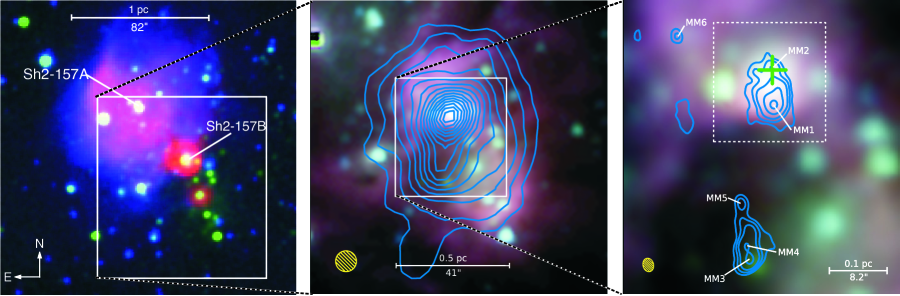
Figure 1.— The Sh2-157 HII massive star forming region over a range of scales and wavelengths. The leftmost panel presents the overview of the entire region with red indicating VLA 3.6 cm emission from ionized gas, green indicating 2MASS K-band $2.2\,\mu$m emission mainly from embedded protostars, and blue showing R-band optical nebulosity and stars from the Digitized Sky Survey. The box shows the region in the center panel which zooms onto the ultra-compact HII region Sh2-157B and accompanying cool, dusty envelope. The background three color image is Spitzer IRAC bands 1,2, 3 ($3.6,4.5,5.8\,\mu$m respectively) and the blue contour overlay shows SCUBA $450\,\mu$m emission. The contour levels begin at, and increment in steps of, 1 Jy beam^-1 and the $7\farcs 5$ SCUBA beamsize is shown as the hashed circle in the lower left corner. The box indicates the region in the rightmost panel which zooms further onto Sh2-157B and the envelope ridge to the south. The background image is the same Spitzer three color image and the blue contour overlays are SMA 1.4 mm emission with levels at $[3,5,8,20,35]\times 1.6$ mJy beam^-1. The $1\farcs 8\times 1\farcs 5$ beamsize is shown as the hashed ellipse in the lower left corner. The green cross indicates the centroid of the VLA 3.6 cm emission.

This region was imaged with the Spitzer Space Telescope as part of a survey of ultra-compact HII regions (PI: Sean Carey). Sh2-157B is a bright, extended source in these data. It also lies at the peak of the SCUBA $450\,\mu$m and $850\,\mu$m maps of Thompson et al. (2006). These submillimeter data show the emission from cool dust in a large cluster envelope. The total integrated $450\,\mu$m flux is 151 Jy which implies a total mass $\sim 700\,M_{\odot}$ (under standard assumptions that are spelled out in §3.1). We plot the archival IRAC and SCUBA data to show the embedded protostellar population in the central panel of Fig 1. The infrared sources mostly lie along a line away from Sh2-157B whereas the envelope extends in a more southerly direction.

The lack of infrared emission along the dense envelope ridge suggests a mass reservoir for continued star formation. In this paper, we present 1.4 mm interferometric observations of the cluster envelope to show its structure at comparable resolution to the optical, infrared, and radio data. We have also carried out ground-based mid-infrared observations of Sh2-157B to obtain higher resolution images than the Spitzer data. We find an elongated structure consisting of three low-mass starless cores in the south and a tight mixture of protostellar evolutionary states in the ultra-compact HII region at the center. This provides new detail into how massive stars and stellar clusters form and also provides an interesting juxtaposition of high and low mass star formation in adjacent regions. Section 2 describes the data acquisition and reduction. Section 3 describes the images and source characterization. We discuss the implications of this work for massive star formation in Section 4 and summarize in Section 5.

2. Observations

We used the Submillimeter Array (SMA) to image the compact condensations within the dusty envelope around Sh2-157B. Observations were carried out in the extended configuration (70–240 meter baselines) on 2008 August 18 and in the compact configuration (20–70 meter baselines) on 2008 September 22. A five pointing Nyquist sampled mosaic was made to provide uniform coverage over the full region of SCUBA emission.

The shape of the bandpass was measured by observing 3C279 and 3C273. The time dependent gains were determined by 5 minute observations of BLLac between 20 minute observations on source. The absolute flux scale was determined from observations of Titan. We used the data reduction package MIR calibrate the visibilities and produced the images using standard MIRIAD routines. The 1.4 mm continuum map was made from the line free channels and spanned 4 GHz in bandwidth (lower plus upper sidebands). The final map was made by inverting the uniformly weighted compact and extended datasets together and has an rms noise level of 1.3 mJy beam^-1 and beamsize $1\farcs 8\times 1\farcs 5$.

The receivers were tuned to place the H₂CO 3_1,2–2_1,1 line at 225.7 GHz in the upper sideband and the DCN 3–2 line at 217.2 GHz in the lower sideband. This was the same setup that proved useful in a similar study of AFGL961 as diagnostics of infall, outflow, and cold core chemistry (Williams et al., 2009). Both these lines were detected in Sh2-157B but we did not find clear evidence for infall or outflow, and they are not used in the analysis described here.

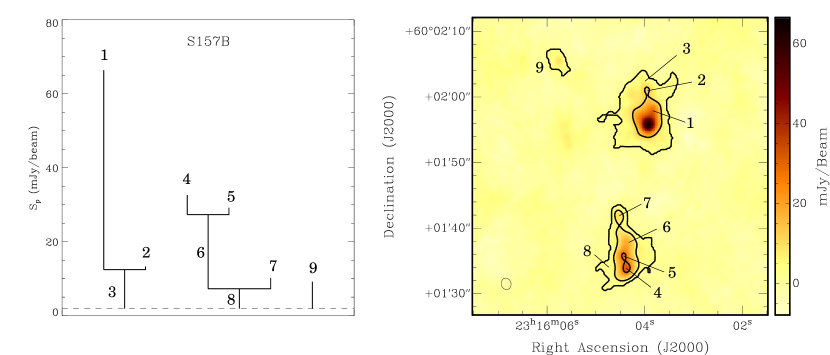
Figure 2.— Dendogram structure decomposition of the SMA 1.4 mm continuum image of S157. The left panel shows the dendogram tree and the right panel labels each feature on the continuum map with contours at break levels between different structures in the dendogram.

We used the mid-infrared camera, MIRSI (Kassis et al., 2008), on the Infrared Telescope Facility (IRTF) to image Sh2-157B at higher resolution and at longer wavelengths than the Spitzer IRAC data. We observed in the N ($10.4\,\mu$m) and Q ($20.9\,\mu$m) filters, on 2009 July 17 to 19 in dry, stable conditions. The images were diffraction limited at $0\farcs 9$ and $1\farcs 7$ resolution respectively. We used a 10^′′ $\times$ 10^′′ dithering pattern and also chopped off the chip with chopping 60^′′ north–south and nodding 90^′′ east–west in order to obtain better sky subtraction in this crowded area. Calibration was performed via observations of $\beta$ Peg throughout the night. The data reduction was performed with an IDL pipeline written by staff astronomer Eric Volquardsen. The plate scale and rotation had been well determined from previous calibration observations and the final images were registered to an absolute astrometric grid by aligning with source 23160401+6002011 in the 2MASS Point Source Catalog that is well detected in both MIRSI bands (and lies at the northeast corner of the leftmost panel of Figure 1.)

3. Results

The SMA continuum emission is shown as contour overlays on the Spitzer IRAC band 3 ($3.5\,\mu$m) image in the rightmost panel of Figure 1. The interferometer spatially filters out much of the envelope and reveals the compact cores within. As with all aspects of the interstellar medium, there is a hierarchy of structures and, even with the spatial filtering, local peaks lie within common regions of extended emission. We first describe the decomposition of the map structure and the resulting bounds to the masses of the compact features and then discuss the relation of the two main groups of sources in the context of their star forming nature.

3.1. Structure decomposition of the millimeter emission

There is an inherent ambiguity in the identification of irregularly shaped objects that overlap in projection or share a common envelope. Visual inspection of the SMA map shows a handful of local peaks nested in two main groups of lower level emission. Based on the nomenclature suggested by Williams et al. (2000), we consider these to be cores within clumps with the connection to star formation being that cores may produce individual stellar systems (single or small order close-multiple) and that clumps are the potential progenitors of stellar groups.

To calculate the properties of the cores and clumps, and their relation to each other, we first decompose the map into a tree network or “dendogram” (Rosolowsky et al., 2008). This reveals nine features which are shown in relation to each in the left panel of Figure 2, and labeled in the image in the right panel. There are three distinct “roots”, one of which (feature 9) is a low level, isolated feature associated with diffuse infrared emission. The other two roots correspond to the two local peaks in the SCUBA $450\,\mu$m map and labeled G111.282–0.665SMM and G111.281–0.670SMM by Thompson et al. (2006). The peaks at the end of these roots are “leaves” and are linked, in one case, by an intermediate hierarchy or ”branch”. Table 1 lists the nine features and their position in the hierarchy, along with basic observational quantities; peak and total intensities, and deconvolved area. Of the six leaves, only two are resolved.

The total intensity of a leaf in Table 1 is the sum above the emission level at which the feature is defined. It therefore provides a minimum mass to the core (this similarly applies to the size). The mass may be considerably higher if we allow for lower level emission from the branches and roots below. The connection to the actual physical properties of the core are less certain in this case but a well defined algorithm, CLUMPFIND, exists to allocate common envelope emission to the local peaks within (Williams et al., 1994). The dendogram analysis provides the emission levels at which the different features separate (“nodes” in the nomenclature of Rosolowsky et al. (2008)) – these are the contours shown in Figure 2 – and we use these as inputs into CLUMPFIND to extend the cores (or “leaves”) to lower levels. This effectively provides an upper limit to the total flux, and therefore maximum mass, to each core.

Table 1Dendogram Structure Analysis

Feature	Type	$F_{\rm peak}$	$F_{\rm total}$	Area
		(mJy/beam)	(mJy)	($\square^{{}^{\prime\prime}}$)
1	Leaf	66.3	177.4	20.0
2	Leaf	13.3	2.9	unresolved
3	Root	66.3	304.4	91.3
4	Leaf	32.6	13.4	unresolved
5	Leaf	29.2	6.4	unresolved
6	Branch	32.6	122.6	23.1
7	Leaf	10.2	5.9	unresolved
8	Root	32.6	180.2	63.4
9	Leaf	9.2	13.0	9.3

Table 2Millimeter Cores

Core	Dendogram	$\alpha$(2000)	$\delta$(2000)	$F_{\rm total}$	$M_{\rm core}$
	Feature	(h:m:s)	(d:m:s)	(mJy)	($M_{\odot}$)
Sh2-157B-MM1	1	23:16:03.93	60:01:56.0	177.4–239.2	12.5–17.0
Sh2-157B-MM2	2	23:16:03.96	60:02:01.0	2.9–25.9	0.2–1.8
Sh2-157B-MM3	4	23:16:04.36	60:01:34.0	13.4–63.9	0.9–4.5
Sh2-157B-MM4	5	23:16:04.43	60:01:35.8	6.4–46.8	0.5–3.3
Sh2-157B-MM5	7	23:16:04.53	60:01:42.0	5.9–14.4	0.4–1.0
Sh2-157B-MM6	9	23:16:05.76	60:02:05.5	13.0	0.9

We calculate the millimeter emitting mass from the SMA 1.4 mm flux, $F_{\rm SMA}$, using the simple, optically thin, relation $M=F_{\rm SMA}d^{2}/\kappa_{\nu}B_{\nu}(T)$, where $d=2.5$ kpc and $B_{\nu}(T)$ is the Planck function. We assume a uniform temperature $T=20K$ and a dust opacity $\kappa_{\nu}=0.1(\nu/1200\,{\rm GHz})$ cm² g^-1 (Hildebrand, 1983) that implicitly includes a gas-to-dust ratio of 100. Although we do not know the dust temperature and opacity for these particular objects, these are typical values for protostellar cores as determined from detailed studies of other regions (e.g., Evans, 1999) and allow for direct comparisons. The positions of the six cores, labeled Sh2-157B-MM1 through Sh2-157B-MM6 and hereafter referred to as MM1 though MM6, are listed in Table 2 along with the range of millimeter fluxes and masses. Because of the blending, the difference between the minimum and maximum mass can be quite large but a clear distinction can nevertheless be made. That is, core MM1 has a mass in excess of $10\,M_{\odot}$ and the other five bracket a solar mass. Their star forming nature is discussed for each clump (dendogram roots 3 and 8) below.

3.2. Protostars and cores in the northern clump

The northern clump, labeled G111.282–0.665SMM by Thompson et al. (2006), is centered on the peak of the SCUBA maps. It has a rising spectrum at infrared wavelengths and is saturated in the Spitzer images in IRAC band 4 ($4.5\,\mu$m) and MIPS bands 1 and 2 (24 and $70\,\mu$m). Our MIRSI N and Q band (10 and $20\,\mu$m) images therefore not only provide higher resolution than the Spitzer data but also the first infrared photometry beyond $8\,\mu$m. The MIRSI data are shown in Figure 3 with a contour overlay of the SMA emission. There are two infrared sources, Sh2-157B-IR1 and Sh2-157B-IR2 (hereafter IR1 and IR2), at $10\,\mu$m and extended emission between them. Both sources are also apparent at $20\,\mu$m but the northernmost source, IR1, is diffuse rather than point-like at this wavelength. IR1 corresponds to the VLA source, i.e., the HII region Sh2-157B, which is similarly extended at 2 cm (Kurtz et al., 1994), and the SMA core MM2. IR2 lies within the SMA contours but is significantly offset from the emission peak, core MM1. We conclude that there are three distinct sources in this region: IR1/MM2 with infrared, millimeter, and radio emission, the infrared source IR2, and the massive core, MM1, that is detected only in the millimeter.

Figure 3.— Mid-infrared MIRSI images resolve Sh2-157B region into two sources IR1 and IR2. The origin of the maps is $\alpha(2000)=23^{\rm h}16^{\rm m}04^{\rm s}.01,\delta(2000)=60^{\circ}02^{\prime}01\farcs 2$. The top panel shows the N-band ($10.6\,\mu$m) image on a linear scale range from 3 to 10 mJy per $0\farcs 27$ pixel. The bottom panel shows the Q–band ($20.9\,\mu$m) image on a linear scale range from 23 to 140 mJy per $0\farcs 27$ pixel. Both panels include blue contour overlays of SMA 1.4 mm emission at $[3,5,8,20,35]\times 1.6$ mJy beam^-1. The blue hashed ellipse in the lower left corner of the bottom panel is the $1\farcs 8\times 1\farcs 5$ SMA beamsize.

Table 3Infrared Sources: Photometry

Source	$\alpha$(2000)	$\delta$(2000)	J	H	K	N	Q
	(h:m:s)	(d:m:s)	(Jy)	(Jy)	(Jy)	(Jy)	(Jy)
Sh2-157B-IR1	23:16:03.96	60:02:01.4	0.015	0.027	0.034	1.0	33.5
Sh2-157B-IR2	23:16:03.71	60:01:57.0	0.002	$<0.019\tablenotemark{a}$	$<0.028$	1.1	13.6

Both IR1 and IR2 have counterparts in the 2MASS catalog and their fluxes from 1.2 to $20.9\,\mu$m are listed in Table 3. The spectral energy distributions (SEDs) are rising throughout this range and, because we do not know where they peak, our interpretation of their nature is limited. A lower limit to their luminosity can be derived by integrating the portion of each SED that is measured, and gives $L_{\rm IR1}>580\,L_{\odot},L_{\rm IR2}>320\,L_{\odot}$. A more realistic estimate comes from comparing the fluxes with the large grid of protostellar models in Robitaille et al. (2007). The 100 lowest $\chi^{2}$ fits have SEDs that peak between 50 and $100\,\mu$m and a mean and standard deviation bolometric luminosity, $L_{\rm IR1}=4200\pm 2200\,L_{\odot},L_{\rm IR2}=1600\pm 700\,L_{\odot}$. Such high luminosities suggest that IR1 and IR2 are massive protostars but the uncertainty in how much of the luminosity is due to accretion prevents us from determining the stellar masses with much precision.

Nevertheless, the diffuse morphology of IR1 at $20\,\mu$m and its association with both millimeter and centimeter emission leads us to conclude that it is a warm, dusty HII region embedded within the cold clump. The integrated 1.3 cm VLA flux toward IR1 is 90 mJy which implies a Lyman continuum flux, $N_{\rm Lyc}=6\times 10^{46}\,{\rm s}^{-1}$, that is a factor of 6 less than an O9.5 star (Martins et al., 2005), and consistent with being an early B star. The low centimeter luminosity is also comparable to many more evolved HII regions that have carved out interstellar bubbles in the Galactic plane (Beaumont & Williams, 2010).

IR2 is about half the luminosity of IR1 and a point source in the near- and mid-infrared. The lack of centimeter emission indicates that it is not a strongly ionizing source. It lies on the edge of the millimeter core and it is therefore hard to place limits on the amount of cool dust around it but it appears to have largely dispersed its own protostellar envelope. We conclude it is likely lower in mass and more evolved than IR1.

The millimeter core itself, MM1, lacks an infrared counterpart at the limits of detection in the MIRSI image. Its proximity to the infrared sources, however, limits how low we can constrain its luminosity from the Spitzer images (see Figure 1) but it is certainly lower than the other Spitzer sources in the region. That is, it has a much lower luminosity than the typical low mass members of the cluster. The core mass lies in the range $12.5-17\,M_{\odot}$ which is much higher than typical low mass star forming cores. Its size and mass imply a surface density $\sim 1$ g cm^-2 that is on the boundary for high mass star formation (Krumholz & McKee, 2008), but unless the efficiency is very high, there is simply not enough mass to form an ionizing star and it may be a progenitor to something more similar to IR2 than IR1.

3.3. Starless cores in the southern clump

Although Thompson et al. (2006) labeled it as a distinct object, G111.281–0.670SMM, the southern clump appears more as an elongation connected to the emission peak in the SCUBA maps. The SMA filters out most of the extended emission and reveals the compact cores within this elongated structure (see the lower half of the rightmost panel in Figure 1).

We identify three distinct cores, labeled MM3–5 in Figure 1, with positions and masses given in Table 2. Their masses are not well determined because of the uncertain contribution from the shared envelope emission but are in the range typical of low mass star forming cores ($M_{\ast}\lesssim 1\,M_{\odot}$) seen in Gould Belt clouds (Sadavoy et al., 2010). They are all unresolved at the $1\farcs 8\times 1\farcs 5$ resolution of these data, implying sizes $\lesssim 4000$ AU, and therefore rough limits on column densities $\gtrsim 10^{22}$ cm^-2, and volume densities $\gtrsim 10^{6}$ cm^-3. These values are high and indicative of objects that are, or shortly will, form stars. None of the cores show detectable infrared emission, however, either in the 2MASS or Spitzer archival images. Comparing these upper limits to the Robitaille et al. (2007). grid of protostellar models, shows that the total luminosity of any embedded sources is less than about $80\,L_{\odot}$, and these are either very young, deeply embedded, relatively low mass ($M_{*}\lesssim 2.5\,M_{\odot}$) protostars or starless cores. It is tempting to speculate that this region will form a small chain of stars, somewhat akin to the angled chain of infrared protostars offset to the west in Figure 1.

4. Discussion

It has been well established that high mass stars tend to form in clusters at the peaks of dense molecular clumps (Zinnecker & Yorke, 2007). Our observations here show two additional luminous objects within a few arcseconds ($<10^{4}$ AU) of the ionizing source of Sh2-157B. One is a luminous, but non-ionizing, protostar and the other is a dense millimeter core with mass $\sim 15\,M_{\odot}$ that is either starless or contains a deeply embedded object. In other words, a cluster is being formed but the individual stars are not born together in perfect synchronicity.

There are also many other lower mass stars visible in the optical and infrared images of the region, as well as apparently low mass, starless cores in the SMA map. The latter, in particular, are found away from the main clump peak at lower average surface densities and with a spatial distribution that follows the elongation of the clump.

The results here resemble our findings from similar MIRSI and SMA imaging of the ultra-compact HII region AFGL961 in the Rosette molecular cloud (Williams et al., 2009) where we also found a compact group of protostars in diverse evolutionary states and a filamentary chain connecting to a starless core. Several other studies using different tracers and looking at different objects find comparable results. For example, Palau et al. (2007) found a cluster of YSOs in the ultra-compact HII region IRAS 20293+3952 with a similar range of infrared-millimeter colors as found here. Although we do not discuss spectral line observations here, these provide many additional ways to delineate evolutionary stages, through signatures of masers, hot and cold core chemistry, core collapse, and protostellar outflows (Beuther et al., 2007; Fontani et al., 2009; Brogan et al., 2009; Palau et al., 2010; Brogan et al., 2011; Wang et al., 2011).

To translate evolutionary states into statistical timescales requires a large systematic survey in much the same way as has been carried out on low mass, more isolated star forming environments (Evans et al., 2009). This would provide a way to assess how star formation depends on the local environment and test models of cluster formation. For example, if Class 0 cores in and around ultra-compact HII regions are found at a similar frequency to those in more isolated regions, then tidal stripping of protostellar envelopes may not be as important as dynamical models of cluster formation suggest (Bate et al., 2003) and would be a point in favor of the picture of quasi-equilibrium cluster formation (Tan et al., 2006).

The tight clustering of sources in a range of evolutionary states show the necessity of arcsecond (or better) resolution images at multiple wavelengths to gain a more complete picture of cluster birth. Ground based infrared imaging to follow up on Spitzer obervations plus sensitive millimeter and centimeter wavelength interferometry provide a powerful combination and promise a bright future as the ALMA and Jansky VLA begin operations.

5. Summary

We have carried out a high resolution, multi-wavelength study of the Sh2-157B region and find evidence for a wide range of protostellar evolutionary states in close proximity to each other. The central ionizing source of the HII region lies at the peak of a massive, dusty clump. Our ground-based mid-infrared imaging and millimeter interferometry show three distinct sources here, all with different infrared-millimeter colors that suggests the individual components of a cluster do not form simultaneously but over an extended, and resolvable, period of time.

Away from the center, we find a chain of three low mass starless cores. These resemble, at an earlier evolutionary stage, a neighboring chain of embedded low luminosity infrared sources that also point back towards the HII region. On these larger scales, then, we also see that different parts of the cluster form at different times and perhaps in coherent structures that derive from the collapsing clump.

These observations are only baby steps toward understanding star formation in clusters. They will soon be greatly superseded by sensitive ALMA observations and, by exploring in more detail the issues raised here, we can begin to place the subject of clustered, high mass star formation on a similar level as our current knowledge of isolated, low mass star formation in nearby clouds.

References

- Bate et al. (2003) Bate, M. R., Bonnell, I. A., & Bromm, V. 2003, MNRAS, 339, 577
- Beaumont & Williams (2010) Beaumont, C. N., & Williams, J. P. 2010, ApJ, 709, 791
- Beuther et al. (2007) Beuther, H., Zhang, Q., Bergin, E. A., Sridharan, T. K., Hunter, T. R., & Leurini, S. 2007, A&A, 468, 1045
- Bonnell & Bate (2006) Bonnell, I. A., & Bate, M. R. 2006, MNRAS, 370, 488
- Bonnell et al. (1998) Bonnell, I. A., Bate, M. R., & Zinnecker, H. 1998, MNRAS, 298, 93
- Brogan et al. (2011) Brogan, C. L., Hunter, T. R., Cyganowski, C. J., Friesen, R. K., Chandler, C. J., & Indebetouw, R. 2011, ApJ, 739, L16
- Brogan et al. (2009) Brogan, C. L., Hunter, T. R., Cyganowski, C. J., Indebetouw, R., Beuther, H., Menten, K. M., & Thorwirth, S. 2009, ApJ, 707, 1
- Chopinet & Lortet-Zuckermann (1972) Chopinet, M., & Lortet-Zuckermann, M. C. 1972, A&A, 18, 373
- Dauphas & Chaussidon (2011) Dauphas, N., & Chaussidon, M. 2011, Annual Review of Earth and Planetary Sciences, 39, 351
- Evans (1999) Evans, II, N. J. 1999, ARA&A, 37, 311
- Evans et al. (2009) Evans, II, N. J., et al. 2009, ApJS, 181, 321
- Fich & Blitz (1984) Fich, M., & Blitz, L. 1984, ApJ, 279, 125
- Fontani et al. (2009) Fontani, F., Zhang, Q., Caselli, P., & Bourke, T. L. 2009, A&A, 499, 233
- Hildebrand (1983) Hildebrand, R. H. 1983, QJRAS, 24, 267
- Israel et al. (1973) Israel, F. P., Habing, H. J., & de Jong, T. 1973, A&A, 27, 143
- Kassis et al. (2008) Kassis, M., Adams, J. D., Hora, J. L., Deutsch, L. K., & Tollestrup, E. V. 2008, PASP, 120, 1271
- Krumholz et al. (2009) Krumholz, M. R., Klein, R. I., McKee, C. F., Offner, S. S. R., & Cunningham, A. J. 2009, Science, 323, 754
- Krumholz & McKee (2008) Krumholz, M. R., & McKee, C. F. 2008, Nature, 451, 1082
- Kurtz et al. (1994) Kurtz, S., Churchwell, E., & Wood, D. O. S. 1994, ApJS, 91, 659
- Kurtz et al. (1999) Kurtz, S. E., Watson, A. M., Hofner, P., & Otte, B. 1999, ApJ, 514, 232
- Lada & Lada (2003) Lada, C. J., & Lada, E. A. 2003, ARA&A, 41, 57
- Martins et al. (2005) Martins, F., Schaerer, D., & Hillier, D. J. 2005, A&A, 436, 1049
- McKee & Ostriker (2007) McKee, C. F., & Ostriker, E. C. 2007, ARA&A, 45, 565
- McKee & Tan (2003) McKee, C. F., & Tan, J. C. 2003, ApJ, 585, 850
- McKee & Williams (1997) McKee, C. F., & Williams, J. P. 1997, ApJ, 476, 144
- Palau et al. (2007) Palau, A., Estalella, R., Girart, J. M., Ho, P. T. P., Zhang, Q., & Beuther, H. 2007, A&A, 465, 219
- Palau et al. (2010) Palau, A., Sánchez-Monge, Á., Busquet, G., Estalella, R., Zhang, Q., Ho, P. T. P., Beltrán, M. T., & Beuther, H. 2010, A&A, 510, A5
- Robitaille et al. (2007) Robitaille, T. P., Whitney, B. A., Indebetouw, R., & Wood, K. 2007, ApJS, 169, 328
- Rosolowsky et al. (2008) Rosolowsky, E. W., Pineda, J. E., Kauffmann, J., & Goodman, A. A. 2008, ApJ, 679, 1338
- Sadavoy et al. (2010) Sadavoy, S. I., et al. 2010, ApJ, 710, 1247
- Sharpless (1959) Sharpless, S. 1959, ApJS, 4, 257
- Tan et al. (2006) Tan, J. C., Krumholz, M. R., & McKee, C. F. 2006, ApJ, 641, L121
- Thompson et al. (2006) Thompson, M. A., Hatchell, J., Walsh, A. J., MacDonald, G. H., & Millar, T. J. 2006, A&A, 453, 1003
- Wang et al. (2011) Wang, Y., et al. 2011, A&A, 527, A32
- Williams (2010) Williams, J. P. 2010, Contemporary Physics, 51, 381
- Williams et al. (2000) Williams, J. P., Blitz, L., & McKee, C. F. 2000, Protostars and Planets IV, 97
- Williams et al. (1994) Williams, J. P., de Geus, E. J., & Blitz, L. 1994, ApJ, 428, 693
- Williams et al. (2009) Williams, J. P., et al. 2009, ApJ, 699, 1300
- Wolfire & Cassinelli (1987) Wolfire, M. G., & Cassinelli, J. P. 1987, ApJ, 319, 850
- Zinnecker & Yorke (2007) Zinnecker, H., & Yorke, H. W. 2007, ARA&A, 45, 481