Nonlinear modal coupling in a high-stress doubly-clamped nanomechanical resonator

Abstract

We present results from a study of the nonlinear intermodal coupling between different flexural vibrational modes of a single high-stress, doubly-clamped silicon nitride nanomechanical beam. The measurements were carried out at 100 mK and the beam was actuated using the magnetomotive technique. We observed the nonlinear behavior of the modes individually and also measured the coupling between them by driving the beam at multiple frequencies. We demonstrate that the different modes of the resonator are coupled to each other by the displacement induced tension in the beam, which also leads to the well known Duffing nonlinearity in doubly-clamped beams.

I Introduction

The nonlinear dynamics of nanoelectromechanical systems (NEMS) has attracted considerable interest over recent years.Blick2002 ; Lifshitz ; Rhoads ; Postma2005 ; aldridge ; kozinsky2 ; buks2 ; kozinsky ; Karabalin2009 ; Westra2010 ; Dunn2010 ; collin Nonlinear behavior is of practical importance in NEMS as it can limit their use as sensors operating in the linear regime,ekinci ; Postma2005 though it also opens up the possibility of devices that are designed to exploit it.aldridge ; guerra However, the very high operating frequencies of NEMS devices (which typically have resonant frequencies in the MHz range) make them ideal for investigating fundamental aspects of nonlinear dynamics.aldridge ; kozinsky ; buks2 ; Karabalin2009 ; Westra2010 ; collin Because NEMS devices are engineered systems and their nonlinearities can be extensively tuned,kozinsky2 it should be possible to use them to study complex nonlinear phenomenacross in which a large number of different mechanical modes interact.buksmems Furthermore, when cooled to very low temperatures, the nonlinear behavior in nanomechanical devices would provide important signatures of the transition from classical to quantum regimes.quantum

Nonlinearity can arise in a wide variety of different ways in NEMS devices.Lifshitz External potentials generated electrostatically by fixed electrodes can be used to induce (or suppress) nonlinear behavior in NEMS.kozinsky2 However, nonlinearities can be intrinsic to a given device or material; for example when a doubly clamped beam is excited its displacement leads to a stretching of the beam which generates a Duffing type nonlinearity in a given mode as well as generating inter-mode couplings.Westra2010 ; Dunn2010 The damping of nanomechanical devices can also be quite nonlinear, something which appears to be particularly important for carbon based devices.eichler

Experiments have begun to explore the coupled nonlinear dynamics of mechanical modes either in two adjacent resonatorsKarabalin2009 or occuring as different harmonics within a single beam.Westra2010 ; Dunn2010 In a recent work Westra et al.Westra2010 explored the nonlinear coupling between the first and third harmonics of a micromechanical doubly clamped beam with mode frequencies in the kHz range. Although the Q-factor of the modes was rather low ($\simeq 10^{2}$) they were able to see clear evidence of nonlinear coupling between the modes induced by the stretching nonlinearity in their beam.

In this paper, we present a systematic study of the nonlinear response of three of the flexural modes of a nanomechanical beam resonator, together with the associated inter-mode couplings. We report the results of a series of measurements taken at 100 mK on the fundamental, third and fifth harmonics (all of which are in the MHz range) of a doubly-clamped beam fabricated from high-stress ($\sim$ 1 GPa) silicon nitride. In a first set of measurements, we excite one mode at a time and find that they display a Duffing like behavior which can be understood quite naturally in terms of the nonlinearity arising from the stretching of the beam. We then measured the response when two modes are driven at the same time, with one mode acting as a probe of the displacement of the other. The high tensile stress and the low temperature mean that the Q-factor of the modes is high enoughsini to allow us to observe the higher mode resonance signals as well as the frequency shifts induced by nonlinear mode-mode couplings which are much larger than the linewidth. Using the single-mode results to calibrate our measuring scheme we are able to make a detailed quantitative comparison (without the need for any fitting parameters) between our results and the predictions of a simple model of the stretching nonlinearity.

This paper is organized as follows. Section II introduces a simple theoretical model of the stretching nonlinearity in beam resonators. The experimental set-up is outlined in Sec. III and in Sec. IV we describe our results. We give our conclusions in Sec. V.

II Theoretical background

Here we review the theoretical description of a beam under tension,Bokaian starting from Euler-Bernoulli equation extended to include the geometric nonlinearity arising from the stretching of the beam that accompanies its flexure.Nayfeh ; Lifshitz For a single mode, this nonlinearity leads naturally to the Duffing equation where a term proportional to the cube of the displacement is added to the usual harmonic equation of motion.Lifshitz However, the non-linearity also generates important couplings between different modes.Westra2010

We start by considering a doubly-clamped beam of length $L$, lying along the $x$-axis, with cross-sectional area $A=wh$, where $w$ is the width and $h$ the thickness. The beam is assumed to be under intrinsic tension, $T_{0}$, and we include, to lowest order, the nonlinear tension arising from the stretching of the beam.Lifshitz The equation of motion for the displacement, $y$, is given by

$$\rho A\ddot{y}+\eta\dot{y}+EI_{y}y^{\prime\prime\prime\prime}-\left[T_{0}+\frac{EA}{2L}\int_{0}^{L}(y^{\prime})^{2}dx\right]y^{\prime\prime}=F_{L},$$ (1)

where $\rho$ is the density, $\eta$ characterizes the damping, $I_{y}=hw^{3}/12$ is the moment of inertia, $F_{L}$ is the force per unit length exerted on the beam and $E$ the Young’s modulus. The non-linearity arises from the second term within the square brackets.

The mode frequencies and mode functions for the corresponding linear problem are knownBokaian and provide a convenient starting point for describing the non-linear regime. If the system is driven harmonically, $F_{L}=F_{n}\cos(\omega_{n}t)$, at a frequency close to one of the linear mode frequencies $\omega_{n,0}$, we can then approximate the displacement of the beam as $y(x,t)=wg_{n}(x)u_{n}(t)$ where $g_{n}(x)$ is the $n$-th mode function, normalized so that $\int_{0}^{1}g_{n}^{2}(\tilde{x})d\tilde{x}=1$ where $\tilde{x}=x/L$.

The dimensionless function $u_{n}(t)$ obeys the equation of motion,Lifshitz

$$\frac{d^{2}u_{n}}{dt^{2}}+\frac{\omega_{n,0}}{Q_{n}}\frac{du_{n}}{dt}+\omega_{n,0}^{2}{u}_{n}+\lambda I_{nn}^{2}{u}_{n}^{3}=f_{n}\cos({\omega}_{n}t),$$ (2)

where $\lambda=(Ew^{2})/(2\rho L^{4})$, $f_{n}=F_{n}\xi_{n}/(hw^{2}\rho)$, with $\xi_{n}=\int_{0}^{1}d\tilde{x}g_{n}(\tilde{x})$ (the mode parameter), and the Q-factor of the $n$-th mode is given by $Q_{n}=\omega_{n,0}(A\rho/\eta)$. The strength of the nonlinearity is controlled by the parameter $I_{nn}$ which is defined by an integral of the form, $I_{ij}=\int_{0}^{1}d\tilde{x}g_{i}^{\prime}(\tilde{x})g_{j}^{\prime}(\tilde{x})$ (with $i$ and $j$ labeling any two modes of the beam).

Since the equation of motion [Eq. 2] is that of the familiar Duffing oscillator, we proceed to analyse it using standard methods.Hand Substituting a solution of the form,

$${u}_{n}=a_{n}\cos({\omega}_{n}t)+b_{n}\sin({\omega}_{n}t),$$ (3)

into Eq. 2, we obtain an equation for the amplitude of the motion, $r_{n}=(a_{n}^{2}+b_{n}^{2})^{1/2}$,

$$r_{n}=f_{n}\left[\left(\omega_{n,0}^{2}+\frac{3}{4}\lambda I_{nn}^{2}r_{n}^{2}-{\omega}_{n}^{2}\right)^{2}+\left(\frac{{\omega}_{n}{\omega}_{n,0}}{Q_{n}}\right)^{2}\right]^{-1/2}.$$ (4)

For a large enough quality factor, $Q_{n}$, and for relatively small amplitudes, $r_{n}$, the main effect of the nonlinearity is to shift the frequency of peak response to

$$\omega_{n,1}=\omega_{n,0}\sqrt{1+\frac{3}{4}\lambda I_{nn}^{2}r_{n}^{2}}.$$ (5)

In the weakly nonlinear regime, the frequency of the resonator shifts from its natural (undriven) value quadratically with increasing amplitude (frequency pulling).Hand ; Nayfeh

We now consider a situation where the drive contains two harmonic components,

$$F_{L}=F_{n}\cos(\omega_{n}t)+F_{m}\cos(\omega_{m}t),$$ (6)

with the two drives frequencies $\omega_{n}$ and $\omega_{m}$ chosen to be close to the resonant frequencies of two different modes, $\omega_{0n}$ and $\omega_{0m}$, respectively. In this case we assume the beam displacement can be approximated as, $y(x,t)=w[u_{n}(t)g_{n}(x)+u_{m}(t)g_{m}(x)]$.

Following the same approach as for the one mode case, assuming $u_{n}$ and $u_{m}$ each oscillate at a single frequency (i.e. they take the form of Eq. 3), we obtain a modified expression for the amplitude of mode $n$,

$$r_{n}=f_{n}\left[\left(\omega_{n,2}^{2}-{\omega}_{n}^{2}\right)^{2}+\left(\frac{{\omega}_{n}{\omega}_{n,0}}{Q_{n}}\right)^{2}\right]^{-1/2}.$$ (7)

where

$$\omega_{n,2}=\omega_{n,0}\sqrt{1+\frac{3}{4}\lambda I_{nn}^{2}r_{n}^{2}+{\lambda}\left(\frac{1}{2}I_{nn}I_{mm}+I_{nm}^{2}\right)r_{m}^{2}.}$$ (8)

Thus we see that the frequency of a given mode depends not just on the amplitude of its own motion, but the amplitude of the other mode that is excited. In particular, the frequency shift of one mode initially grows quadratically with the amplitude of the other one.

III Experimental Set-up

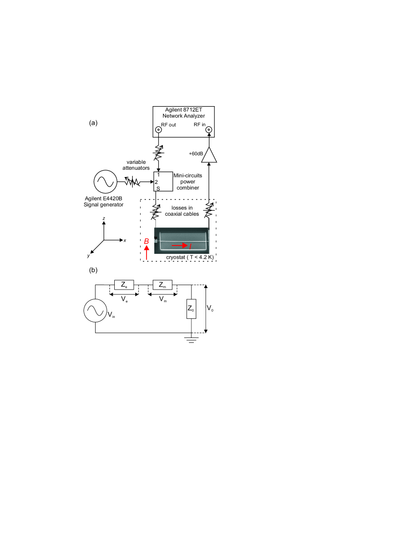
Figure 1: (a) Schematic diagram of the measurement set-up. The different modes of the beam were driven with two separate signal generators. A voltage signal proportional to the emf generated by the beam was detected at the input of the network analyzer after passing through a pre-amplifier. (b) Circuit model for transmission measurements, with external circuit impedances $Z_{e}$ and $Z_{0}$, sample impedance $Z_{m}$, the drive voltage $V_{\mathrm{in}}$ and the measured voltage $V_{0}$.

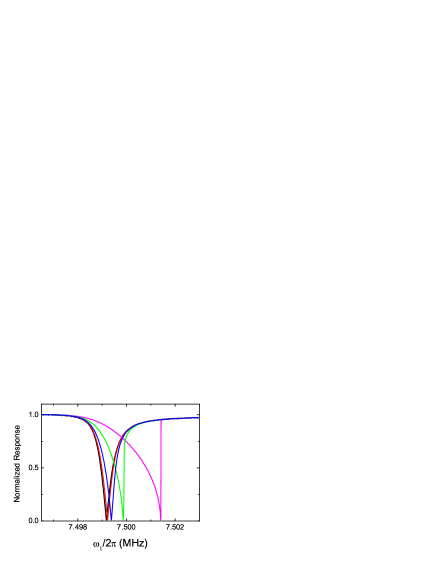
Figure 2: Resonant response of mode 1 (7.5 MHz). The curves from left to right correspond to a series of increasing drive strengths. The normalized response consists of the measured voltage, $V_{a1}$, scaled by the maximum value measured in each case.

Experiments were performed on a silicon nitride beam with length $25.5$ $\mu$m, width $170$ nm and thickness $170$ nm. Metal layers consisting of 3 nm of Ti and $40$ nm of Au were added by thermal deposition to form a wire on top of the beam through which a drive current could be applied. The devices were fabricated by dry-etching in a multi-stage processKunal_thesis from wafers composed of a 190 $\mu$m thick silicon wafer with 170 nm of silicon nitride on both sides; the nitride layer has a built-in tensile stress of about $1070$ MPa at room temperature.cornell

A schematic diagram of the experimental set-up is shown in Fig. 1a. The resonator was placed inside a ³He/⁴He dilution refrigerator and measurements were performed at $100$ mK. The motion of the beam was monitored using the the magnetomotive method.Cleland1999 A magnetic field of $B=3$ T was applied and the drive was applied by passing an alternating current through the sample. The response to the resulting Lorentz force was detected by measuring a voltage ($V_{a}$), which is related to the input voltage at the rf pre-amplifier ($V_{0}$), as the frequency of the drive signal was tuned through the mechanical resonance. The beam was driven at two different frequencies by using an additional signal generator as shown in Fig. 1a. The measurements were carried out in transmission mode, see Fig. 1b, capturing a dip in the conductance of the beam in the spectral domain.

The motion of the resonator in the magnetic field generates an emf,Cleland1999 which itself is related to the mechanical motion. Provided that the resonances are well-resolved, $|\omega_{0m}-\omega_{0n}|\gg\frac{\omega_{0m}}{Q_{m}}+\frac{\omega_{0n}}{Q_{n}}$, for $m\neq n$, the motion at a given frequency can be attributed to a single mode and

$$V_{\mathrm{emf}}=w\xi_{n}LB\frac{\partial{u}_{n}}{\partial{t}}.$$ (9)

We can relate the final measured voltage, $V_{an}$ to $V_{\mathrm{emf}}$, and hence to the amplitude of a given mode, $r_{n}$, by applying Kirchoff’s law to the circuit (Fig. 1b) and solving the corresponding equations. Thus we find,

$$V_{an}=GV_{0}=\frac{Z_{0}G}{Z_{0}+Z_{e}}\left(V_{\mathrm{in}}-V_{\mathrm{emf}}\right),$$ (10)

where $G$ is a constant of proportionality that quantifies the overall signal gain from the sample to the network analyzer, taking into account the losses in the transmission cables as well as the gain provided by the amplifiers. The gain in the transmission line will in fact vary slightly with frequency (hence the gain will not be the same for different modes) and local temperature variations inside the fridge. Mechanical resonance leads to a dip in the voltage $V_{an}$, hence (assuming the circuit impedances are real) we can characterize the mechanical response of a particular mode by,

$$V_{Sn} = |\frac{Z_{0}G}{Z_{0}+Z_{e}}V_{\mathrm{in}}-V_{an}|$$ (11)

$$= \frac{Z_{0}}{Z_{0}+Z_{e}}GBLw\xi_{n}\omega_{n}r_{n},$$

which measures the size of the dip. Expanding Eq. 5 to lowest order in $r_{n}$ and using Eq. 11 leads to the explicit expression:

$$\omega_{n,1}=\omega_{n,0}+\alpha_{n}V_{Sn}^{2},$$ (12)

where $\alpha_{n}=\frac{3I_{nn}^{2}\lambda\omega_{n,0}D_{n}}{8(BL\omega_{n}\xi w)^{2}}$ and $D_{n}=\left(\frac{Z_{0}+Z_{e}}{Z_{0}}\frac{1}{G}\right)^{2}$.

IV Results

We were able to detect the first three odd harmonics of the beam which had frequencies 7.5, 22.85 and 39.28 MHz respectively (the even modes do not give rise to a signal which is directly measurable using the magnetomotive method). Measurements on each individual mode were performed first, capturing the response of the resonator as the driving frequency was swept through the mechanical resonant frequency. The basic properties of the three modes are summarized in Table I. The frequencies are those measured at the lowest drive levels used. The Q-factors are the measured values at a field of 3 T. Although the values are still rather high, the relatively strong magnetic field used means that they are lower than the intrinsic Q-factors of the modesCleland1999 (much lower in the case of the $n=1$ modeKunal_thesis whose intrinsic Q-factor is $1.8\times 10^{6}$ at 100 mK).

The nonlinear parameters, $I_{nn}$, and the mode parameters, $\xi_{n}$, are calculated numerically using a value of the intrinsic tension which we estimate to be $T_{0}=1020$ MPa. This is slightly lower than the room temperature value because of the different thermal contractions of the silicon and silicon nitride layers in the wafer.Kunal_thesis The parameters, $I_{nn}$, and hence the strength of the nonlinearity in a given mode, grow rapidly in size with the mode number $n$. The cross terms, $I_{nm}$, which involve two different modes, also grow with the mode number, but are much smaller for our device: $I_{13}=-1.9$, $I_{15}=-3.0$, and $I_{35}=-8.8$. In calculating the parameter $\lambda=(Ew^{2})/(2\rho L^{4})$ we use the Young’s modulus of silicon nitridethesis80 $E_{SiN}=211$ GPa and neglect the contribution from the gold as it is under much less tension and its Young’s modulus, $E_{Au}=78$ GPa, is smaller. We include the effect of the gold layer on the mass by using an appropriate average value for the density. Using these parameters we obtain theoretical estimates of the three mode frequencies of $7.8$, $24.2$ and $42.5$ MHz respectively which are all close to the measured values (given in Table 1). The discrepancies between estimated and measured frequencies arise from the uncertainties in the device dimensions ($L\sim\pm 1\%$, $w\sim\pm 5\%$ and $t_{Au}\sim\pm 10\%$).

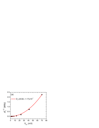
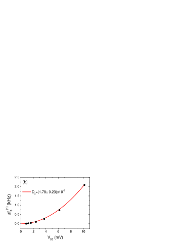
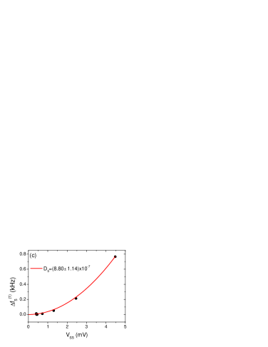
Figure 3: Shift in the frequency, $\Delta f_{n}^{(1)}$, as a function of the voltage $V_{Sn}$ for (a) $n=1$, (b) $n=3$, and (c) $n=5$. The points are the data and the lines are quadratic fits. The corresponding values of the parameters $D_{n}$ obtained from the fit, together with the associated uncertainty, are given in each case.

n	$\omega_{0n}/2\pi$ (MHz)	$\xi_{n}$	$I_{nn}$	$Q_{n}$
1	7.50	0.88	10.4	$9.0\times 10^{3}$
3	22.85	0.30	93.3	$1.7\times 10^{5}$
5	39.28	0.19	257.9	$4.1\times 10^{5}$

Table 1: Properties of the three measured modes of the silicon nitride beam.

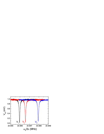
Figure 4: Response curves of the third flexural mode for different measured voltages, $V_{S1}$, at the frequency of the first mode, $V_{1}=15.2$ mV, $V_{2}=29.3$ mV and $V_{3}=48$ mV, corresponding to three successively increasing drive amplitudes applied at a fixed frequency of 7.499 MHz.

Data were collected for a range of drive amplitudes by systematically increasing the drive signal. As an example, the spectral response of the fundamental mode is shown in Fig. 2 as a function of the corresponding drive amplitude. As expected, the curves are symmetric for the smallest drives, but become increasingly asymmetric as the beam is driven harder. At the largest amplitudes, the device enters a strongly nonlinear regime marked by sharp changes seen in the measured signal on the high frequency side of the resonance.foot1 Frequency pulling is also clearly visible, with the peak frequency of each mode shifting upwards as the drive is increased. Very similar behavior is seen for modes 3 and 5.

Figure 5: Frequency shifts of (a) the fifth mode, $\Delta f^{(2)}_{5}$, and (b) the third mode $\Delta f^{(2)}_{3}$, as a function of the measured response of the first mode, $V_{S1}$, to a sequence of progressively stronger drives. In each case the points are data, and the shaded area is the band of values consistent with theoretical predictions when uncertainties in the parameters are accounted for.

Figure 6: Frequency shifts of (a) the fifth mode, $\Delta f^{(2)}_{5}$, and (b) the first mode $\Delta f^{(2)}_{1}$, as a function of the measured response of the third mode, $V_{S3}$, to a sequence of progressively stronger drives. In each case the points are data, and the shaded area is the band of values consistent with theoretical predictions when uncertainties in the parameters are accounted for.

We extracted the frequencies of peak response, $f_{n}^{(1)}=\omega_{n,1}/2\pi$ and the corresponding voltages $V_{Sn}$ from the measured resonance curves (Fig. 2). The shift in peak frequency, $\Delta f_{n}^{(1)}=(\omega_{n,1}-\omega_{n,0})/2\pi$, versus peak measured voltage $V_{Sn}$, for each mode is shown in Fig. 3. Theory predicts (see Eq. 12) that the frequency shift should increase quadratically with the voltage and this is what is found. All the parameters required for the analysis are known (with stated uncertainty) except for the $D_{n}$. We obtain a value of the quadratic coefficient, $\alpha_{n}$, for each mode by fitting each set of measured data to a quadratic function with a fitting error of less than 3%, from which we then calculate the $D_{n}$. The fits are shown as lines in Fig. 3. The value of $D_{n}$ varies between the modes by about a factor of two, due to the intrinsic frequency dependence of the circuit impedances and amplifier gain. The error in $D_{n}$ is about 13$\%$ and follows directly from the error in sample dimensions.

Next we probed the interactions between the different modes of the beam by exciting one mode weakly and measuring its response as successively stronger drive amplitudes (of a fixed frequency) were applied to a second mode. The shift in the peak response frequency of the weakly driven mode, $\Delta f_{n}^{(2)}=(\omega_{n,2}-\omega_{n,0})/2\pi$, was measured together with the voltage at the frequency of the second mode. Response curves for mode 3, measured for three different levels of drive applied to mode 1, is shown in Fig. 4. As expected, the resonant frequency of mode 3 increases with the measured voltage from the first mode. Looking at the depths of the curves in Fig. 4, we see that increasing the amplitude of the mode 1 drive reduces the amplitude of the response of mode 3 slightly.Westra2010 A reduction in the peak amplitude is a natural consequence of an increase in the frequency $\omega_{n,2}$ [see Eq. 7], but we also find a very slight degradation in the Q-factor of the third mode accompanies the increasing drive at the fundamental frequency.

Figure 7: Amplitude of the motion of mode 1 (at the antinode), $A_{1}$, as a function of the drive frequency $\omega_{1}/2\pi$ obtained using the frequency shift in mode 3. Each point is generated by measuring a full frequency response curve for mode 3 and the obtaining the resulting $\Delta f^{(2)}_{3}$ which is then converted into an amplitude.

The shift in the peak response frequencies of the third and fifth modes as a function of the voltage measured at the frequency of mode 1, $V_{S1}$, are shown in Fig. 5. Similarly, Fig. 6 shows the effect of varying the amplitude of the third mode on the resonant frequency of the first and fifth modes. Again the theory predicts (through Eqs. 8 and 11) a quadratic dependence of the frequency shifts on the measured voltages. However, because the values of the parameters $\alpha_{n}$ have been determined from fits to the single-mode data, the comparison with theory now involves no free parameters. We use the $\alpha_{n}$ values extracted from the single mode data, and the parameters $I_{nm}$, together with the associated uncertainties, to plot shaded bands in Figs. 5 and 6 showing the regions which are fully consistent with the theory. We note that the $I_{nm}$ values are quite insensitive to the changes in beam dimensions, so the predictions of the theory are fairly precise. In each case it is clear that the dependence of the frequency shifts on the voltages is well described by a quadratic law, and that there is very good agreement between the theoretical predictions and the measurements.

Having verified that the bending nonlinearity provides a quantitatively accurate description of the modal couplings in the beam, we can now obtain the amplitude of the motion in one mode by measuring the frequency shifts in a second (weakly driven) mode. The theoretical expression, Eq. 8, and the mode function $g_{n}(x)$ allow us to convert from a measured frequency shift to a physical amplitude at a given point along the beam. An example is shown in Fig. 7 in which the amplitude of mode 1 at the antinode $x=L/2$, obtained by measuring a frequency shift in mode 3, is shown as a function of the drive frequency, $\omega_{1}$. An amplitude of 1 nm in mode 1 translates into a frequency shift in mode 3 of $7.11$ Hz, a factor of $\sim 40$ larger than that observed in Ref. Westra2010, . From Fig. 7 we see that an amplitude of 25 nm ($\sim 10$% of the width of the beam) is already well within the non-linear regime.

V Conclusions

We have measured the properties of three of the flexural modes of a highly stressed, doubly-clamped silicon nitride nanomechanical beam. The size of the sample, the Q-factors, the temperature and the degree of non-linearity are all orders of magnitude different than reported by Westra et al. Westra2010 for an unstressed beam at room temperature. As a first step we investigated the frequency pulling that accompanies increases in the drive applied to each of the modes in turn. For all three modes the frequency was found to grow quadratically with the amplitude of the motion, consistent with the Duffing-type behavior predicted for a nonlinearity governed by the stretching of the beam on deflection.

We then examined the behavior of the system when one mode is driven weakly and the amplitude of the drive applied to a second mode is increased steadily. We again found that the frequency of the weakly driven mode increased quadratically, this time with the amplitude of the second mode. Using the results from the single-mode experiments to calibrate our measurement set-up we were able to make a comparison without any free parameters to theoretical predictions. The good agreement we find using four different pairs of modes allows us to conclude that the nonlinear dynamics we observe does indeed arise from the stretching of the beam on deflection.

In conclusion, our data confirm that the bending nonlinearity provides a good quantitative description of the mode couplings in our nanomechanical device. We find that beam starts to behave nonlinearly for amplitudes that are a small fraction of its width, which means that the system has a high intrinsic nonlinearity due to its size and the built-in stress in the nitride layer. Furthermore, our measurements also allows us to calculate the physical displacement of one mode by measuring a frequency shift in a second mode. Studying the inter-modal couplings in nanomechanical beams is of great importance for understanding the dynamics of such small systems, and can be of great use to device applications or fundamental studies which require a combination of high frequencies, large $Q$-factors and sensitivity.

References

- (1) R. H. Blick, A. Erbe, L. Pescini, A. Kraus, D. V. Scheible, F. W. Beil, E. Hoehberger, A. Hoerner, J. Kirschbaum, H. Lorenz, and J. P. Kotthaus, J. Phys. Condens. Matter 79, 905 (2002).
- (2) R. Lifshitz and M. C. Cross, Reviews of Nonlinear Dynamics and Complexity, edited by H. G. Schuster (Wiley, Weinheim, 2008), Chap. 1., p. 52.
- (3) J. F. Rhoads, S. W. Shaw and K. L. Turner, J. Dynamic Systems, Measurement and Control 132, 034001 (2010).
- (4) H. W. Ch. Postma, I. Kozinsky, A. Husain, and M. L. Roukes, Appl. Phys. Lett. 86, 223105 (2005).
- (5) J. S. Aldridge and A. N. Cleland, Phys. Rev. Lett. 94, 156403 (2005).
- (6) I. Kozinsky, H. W. Ch. Postma, I. Bargatin and M. L. Roukes, Appl. Phys. Lett. 88, 253101 (2006).
- (7) R. Almog, S. Zaitsev, O. Shtempluck, and E. Buks, Appl. Phys. Lett. 88, 213509 (2006).
- (8) I. Kozinsky, H. W. Ch. Postma, O. Kogan, A. Husain and M. L. Roukes, Phys. Rev. Lett. 99, 207201 (2007).
- (9) R. B. Karabalin, M. C. Cross, and M. L. Roukes, Phys. Rev. B 79, 165309 (2009).
- (10) H. J. R. Westra, M. Poot, H. S. J. van der Zant, and W. J. Venstra, Phys. Rev. Lett. 105, 117205 (2010).
- (11) T. Dunn, J-S. Wenzler, and P. Mohanty, App. Phys. Lett. 97, 123109 (2010).
- (12) E. Collin, Yu. M. Bunkov and H. Godfrin, Phys. Rev. B 82, 235416 (2010).
- (13) K. L. Ekinci and M. L. Roukes, Rev. Sci. Instruments 76, 061101 (2005).
- (14) D. N. Guerra, A. R. Bulsara, W. L. Ditto, S. Sinha, K. Murali, and P. Mohanty, Nano Lett 10, 1168 (2010).
- (15) M. C. Cross, A. Zumdieck, R. Lifshitz, and J. L. Rogers, Phys. Rev. Lett. 93, 224101 (2004).
- (16) E. Buks and M. L. Roukes, J. MEMS 11, 802 (2002).
- (17) I. Katz, A. Retzker, R. Straub and R. Lifshitz, Phys. Rev. Lett. 99, 040404 (2007).
- (18) A. Eichler, J. Moser, J. Chaste, M Zdrojek, I. Wilson-Rae and A. Bachtold, Nature Nano. 6, 339 (2011).
- (19) S. S. Verbridge, D. Finkelstein-Shapiro, H. G. Craighead, and J. M. Parpia, Nano Lett. 7, 1728 (2007).
- (20) A. Bokaian, J. Sound and Vibration 142, 481 (1990).
- (21) L. N. Hand and J. D. Finch, Analytical Mechanics (Cambridge University Press, Cambridge, UK, 1998).
- (22) A. H. Nayfeh and D. T. Mook, Nonlinear Oscillations (John Wiley & Sons, New York, 1979).
- (23) The silicon nitride layers were deposited on the silicon substrates using a low pressure chemical vapour deposition (LPCVD) process at the Cornell Nanoscale Science and Technology Facility (CNF), 250 Duffield Hall, Cornell University, Ithaca, New York, USA.
- (24) A. N. Cleland and M. L. Roukes, Sens. and Actuators A 72, 256 (1999).
- (25) M. Poot, PhD thesis (Technische Universiteit Delft, 2009), unpublished.
- (26) K. Lulla, PhD thesis (University of Nottingham, 2011), unpublished.
- (27) W-H. Chuang, J. MEMS, 13, 870 (2004).
- (28) Note that when these measurements were taken the frequency was always swept upwards.