Chemical-Potential Route: A Hidden Percus–Yevick Equation of State for Hard Spheres

Abstract

The chemical potential of a hard-sphere fluid can be expressed in terms of the contact value of the radial distribution function of a solute particle with a diameter varying from zero to that of the solvent particles. Exploiting the explicit knowledge of such a contact value within the Percus–Yevick (PY) theory, and using standard thermodynamic relations, a hitherto unknown PY equation of state, $p/\rho k_{B}T=-(9/\eta)\ln(1-\eta)-(16-31\eta)/2(1-\eta)^{2}$, is unveiled. This equation of state turns out to be better than the one obtained from the conventional virial route. Interpolations between the chemical-potential and compressibility routes are shown to be more accurate than the widely used Carnahan–Starling equation of state. The extension to polydisperse hard-sphere systems is also presented.

Motivation and discussion.—

As is well known, the hard-sphere (HS) model is of great importance in condensed matter, colloids science, and liquid state theory from both academic and practical points of view Hansen and McDonald (2006); Likos (2001); Mulero (2008). The model has also attracted a lot of interest because it provides a nice example of the rare existence of nontrivial exact solutions of an integral-equation theory, namely the Percus–Yevick (PY) theory Percus and Yevick (1958) for odd dimensions Wertheim (1963, 1964); Thiele (1963); Lebowitz (1964); Freasier and Isbister (1981); Leutheusser (1984); Robles et al. (2004, 2007); Rohrmann and Santos (2007, 2011a, 2011b).

As generally expected from an approximate theory, the radial distribution function (RDF) provided by the PY integral equation suffers from thermodynamic inconsistencies; i.e., the thermodynamic quantities derived from the same RDF via different routes are not necessarily mutually consistent. In particular, the PY solution for three-dimensional one-component HSs of diameter $\sigma$ yields the following expression for the compressibility factor $Z\equiv p/\rho k_{B}T$ (where $p$ is the pressure, $\rho$ is the number density, $k_{B}$ is Boltzmann’s constant, and $T$ is the temperature) through the virial (or pressure) route Wertheim (1963, 1964); Thiele (1963):

$$Z_{\text{PY-}v}(\eta)=\frac{1+2\eta+3\eta^{2}}{(1-\eta)^{2}}.$$ (1)

Here, $\eta=\frac{\pi}{6}\rho\sigma^{3}$ is the packing fraction and the subscript $v$ is used to emphasize that the result corresponds to the virial route. In contrast, the compressibility route yields

$$Z_{\text{PY-}c}(\eta)=\frac{1+\eta+\eta^{2}}{(1-\eta)^{3}}.$$ (2)

Equation (2) is also obtained from the scaled-particle theory (SPT) Reiss et al. (1959); Mandell and Reiss (1975); Heying and Corti (2004). The celebrated and accurate Carnahan–Starling (CS) Carnahan and Starling (1969) equation of state (EOS) is obtained as the simple interpolation

$$Z_{\text{CS}}(\eta) = \frac{1}{3}Z_{\text{PY-}v}(\eta)+\frac{2}{3}Z_{\text{PY-}c}(\eta)$$ (3)

$$= \frac{1+\eta+\eta^{2}-\eta^{3}}{(1-\eta)^{3}}.$$

For general interaction potentials, the third conventional route to the EOS is the energy route Hansen and McDonald (2006). However, this route is useless in the case of HSs since the internal energy is just that of an ideal gas, and thus it is independent of density. On the other hand, starting from a square-shoulder interaction and then taking the limit of vanishing shoulder width, it has been proved that the resulting HS EOS coincides exactly with the one obtained through the virial route, regardless of the approximation used Santos (2005, 2006). Therefore, the energy and virial routes to the EOS can be considered as equivalent in the case of HS fluids.

Table 1: First ten virial coefficients $b_{n}$ as obtained exactly and from several EOS related to the PY theory.

$n$	Exact	$Z_{\text{PY-}v}$	$Z_{\text{PY-}c}$	$Z_{\text{PY-}\mu}$	$Z_{\text{CS}}$	$Z_{\mu c,1}$	$Z_{\mu c,2}$
${2}$	4	$4$	$4$	$4$	$4$	$4$	$4$
${3}$	$10$	$10$	$10$	$10$	$10$	$10$	$10$
${4}$	$18.36476\ldots$	$16$	$19$	$16.75$	$18$	$18.1$	$18.125$
${5}$	$28.2245$	$22$	$31$	$23.8$	$28$	$28.12$	$28.2$
${6}$	$39.815$	$28$	$46$	$31$	$40$	$40$	$40.166\ldots$
${7}$	$53.34$	$34$	$64$	$38.285714\ldots$	$54$	$53.714285\ldots$	$54$
${8}$	$68.54$	$40$	$85$	$45.625$	$70$	$69.25$	$69.6875$
${9}$	$85.81$	$46$	$109$	$53$	$88$	$86.6$	$87.222\ldots$
${10}$	$105.8$	$52$	$136$	$60.4$	$108$	$105.76$	$106.6$

Except perhaps in the context of the SPT Reiss et al. (1959); Mandell and Reiss (1975); Heying and Corti (2004), little attention has been paid to a fourth route to the EOS of HSs: the chemical-potential route not (a). In particular, to the best of the author’s knowledge, the possibility of obtaining the EOS via this route by exploiting the exact solution of the PY equation for HS mixtures Lebowitz (1964) seems to have been overlooked. The main aim of this Letter is to fill this gap and derive the results

$$\frac{\mu_{\text{PY}}^{\text{ex}}(\eta)}{k_{B}T}=7\eta\frac{1+\eta/14}{(1-\eta)^{2}}-\ln(1-\eta),$$ (4)

$$Z_{\text{PY-}\mu}(\eta)=-9\frac{\ln(1-\eta)}{\eta}-8\frac{1-\frac{31}{16}\eta}{(1-\eta)^{2}},$$ (5)

where $\mu^{\text{ex}}$ is the excess chemical potential and the subscript $\mu$ in Eq. (5) denotes that the compressibility factor is obtained from Eq. (4). Equation (5) differs from Eqs. (1) and (2) in that it includes a logarithmic term and thus it is not purely algebraic. Nevertheless, $Z_{\text{PY-}\mu}(\eta)$ is analytic at $\eta=0$ and provides well-defined values for the (reduced) virial coefficients $b_{n}$ defined by

$$Z(\eta)=1+\sum_{n=2}^{\infty}b_{n}\eta^{n-1}.$$ (6)

Table 1 compares the first ten virial coefficients obtained from the three PY EOS, Eqs. (1), (2), and (5), with the exact analytical ($n=2$–$4$) and Monte Carlo ($n=5$–$10$) values Labík et al. (2005); Clisby and McCoy (2006). The interpolated coefficients obtained from Eq. (3) are also included. We observe that the virial coefficients $b_{n}^{(\text{PY-}\mu)}$ obtained from Eq. (5) are in general noninteger rational numbers. More explicitly, $b_{n}^{(\text{PY-}\mu)}=(18-31n+15n^{2})/2n$, while $b_{n}^{(\text{PY-}v)}=2(3n-4)$, $b_{n}^{(\text{PY-}c)}=(3n^{2}-3n+2)/2$, and $b_{n}^{(\text{CS})}=(n+2)(n-1)$.

Interestingly enough, the virial coefficients from the chemical-potential route are more accurate than those from the virial route, although less than the ones from the compressibility route. This suggests the possibility of exploring CS-like interpolations of the form $Z_{\mu c}(\eta)=\alpha Z_{\text{PY-}\mu}(\eta)+(1-\alpha)Z_{\text{PY-}c}(\eta)$ with $\alpha\approx 0.4$. Two simple and convenient choices are $\alpha=\frac{2}{5}$ and $\alpha=\frac{7}{18}$. Thus,

$$Z_{\mu c,1}(\eta) = \frac{2}{5}Z_{\text{PY-}\mu}(\eta)+\frac{3}{5}Z_{\text{PY-}c}(\eta)$$ (7)

$$= -\frac{18}{5}\frac{\ln(1-\eta)}{\eta}-\frac{13-50\eta+28\eta^{2}}{5(1-\eta)^{3}},$$

$$Z_{\mu c,2}(\eta) = \frac{7}{18}Z_{\text{PY-}\mu}(\eta)+\frac{11}{18}Z_{\text{PY-}c}(\eta)$$ (8)

$$= -\frac{7}{2}\frac{\ln(1-\eta)}{\eta}-\frac{30-117\eta+65\eta^{2}}{12(1-\eta)^{3}}.$$

The values $b_{n}^{(\mu c,1)}=(36-56n+21n^{2}+9n^{3})/10n$ and $b_{n}^{(\mu c,2)}=(42-65n+24n^{2}+11n^{3})/12n$ obtained from Eqs. (7) and (8), respectively, are also displayed in Table 1. We observe a very good agreement, even better than that of $b_{n}^{(\text{CS)}}$, with the exact values, especially in the case of $b_{n}^{(\mu c,1)}$. In particular, $b_{10}^{(\mu c,1)}$ is excellent.

The superiority of $Z_{\mu c,1}$ and $Z_{\mu c,2}$ over $Z_{\text{CS}}$ is confirmed by Fig. 1, where the differences $Z_{\text{CS}}(\eta)-Z_{\text{MD}}(\eta)$, $Z_{\mu c,1}(\eta)-Z_{\text{MD}}(\eta)$, and $Z_{\mu c,2}(\eta)-Z_{\text{MD}}(\eta)$ (where $Z_{\text{MD}}$ denotes molecular dynamics simulation values Kolafa et al. (2004)) are compared. As can be seen, both $Z_{\mu c,1}$ and $Z_{\mu c,2}$ deviate from $Z_{\text{MD}}$ less than $Z_{\text{CS}}$ over most of the stable liquid region. It is noteworthy that, while $Z_{\mu c,1}$ predicts better virial coefficients than $Z_{\mu c,2}$, the latter EOS is more accurate for $\eta>0.1$.

In the case of a polydisperse HS fluid characterized by a size distribution $x(\sigma^{\prime})$, it will be proved elsewhere not (b) that Eqs. (4) and (5) are generalized to

$$\frac{\mu_{\text{PY}}^{\text{ex}}(\eta,\sigma)}{k_{B}T} = -\ln(1-\eta)+\frac{\eta}{1-\eta}\left[\frac{\sigma^{3}}{M_{3}}+3\frac{M_{1}\sigma^{2}}{M_{3}}\right.$$ (9)

$$\left(1+\frac{\eta}{1-\eta}\frac{M_{2}\sigma}{M_{3}}\right)+3\frac{M_{2}\sigma}{M_{3}}$$

$$\left.\times\left(1+\frac{3}{2}\frac{\eta}{1-\eta}\frac{M_{2}\sigma}{M_{3}}\right)\right],$$

$$Z_{\text{PY-}\mu}(\eta) = \frac{1}{1-\eta}+\frac{M_{1}M_{2}}{M_{3}}\frac{3\eta}{(1-\eta)^{2}}-9\frac{M_{2}^{3}}{M_{3}^{2}}$$ (10)

$$\times\left[\frac{\ln(1-\eta)}{\eta}+\frac{1-\frac{3}{2}\eta}{(1-\eta)^{2}}\right],$$

where $M_{n}\equiv\int_{0}^{\infty}\text{d}\sigma^{\prime}\,x(\sigma^{\prime})\sigma^{\prime n}$ is the $n$th moment of the size distribution and in Eq. (9) $\mu_{\text{PY}}^{\text{ex}}(\eta,\sigma)$ is the excess chemical potential of spheres of diameter $\sigma$. Equation (10) differs from $Z_{\text{PY-}v}$ and $Z_{\text{PY-}c}$ for mixtures Lebowitz (1964) only by the coefficient of $M_{2}^{3}/M_{3}^{2}$. Analogously to the one-component case, it is possible to construct interpolated EOS $Z_{\mu c}=\alpha Z_{\text{PY-}\mu}+(1-\alpha)Z_{\text{PY-}c}$, with $\alpha=\frac{2}{5}$ or $\alpha=\frac{7}{18}$, which are more accurate than the Boublík–Mansoori–Carnahan–Starling–Leland EOS Boublík (1970); Mansoori et al. (1971).

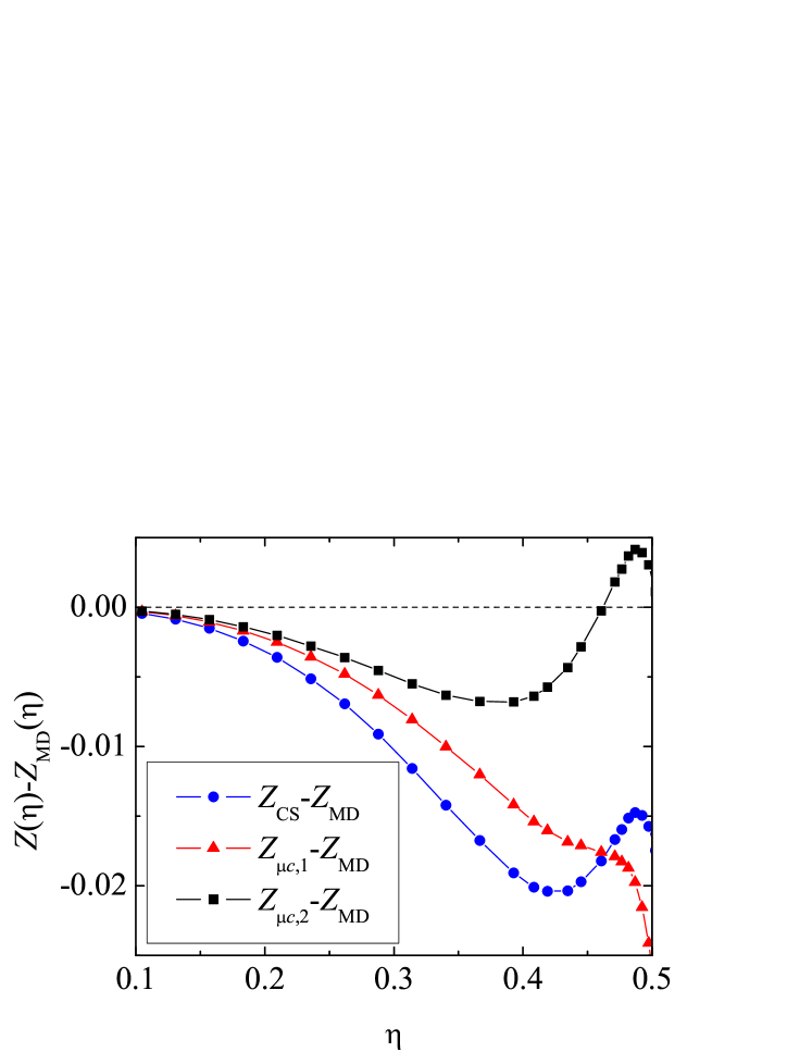
Figure 1: (color online). Plot of $Z_{\text{CS}}(\eta)-Z_{\text{MD}}(\eta)$ (circles), $Z_{\mu c,1}(\eta)-Z_{\text{MD}}(\eta)$ (triangles), and $Z_{\mu c,2}(\eta)-Z_{\text{MD}}(\eta)$ (squares).

Once the main features and applications of the new PY EOS (5) have been discussed, the rest of the Letter is devoted to its derivation.

The chemical-potential route.—

Let us consider a $d$-dimensional system made of $N$ hard spheres ($i=1,\ldots,N$) of diameter $\sigma$ (the “solvent”) plus one “solute” particle ($i=0$) which interacts with the solvent particles via a HS potential of core $\lambda\sigma$ with $0\leq\lambda\leq 1$. Thus, the total potential energy function is

$$\Phi_{N+1}(\mathbf{r}^{N+1};\lambda) \equiv \Phi_{N+1}(\mathbf{r}_{0},\mathbf{r}_{1},\ldots,\mathbf{r}_{N};\lambda)$$

$$= \sum_{j=1}^{N}\phi_{\text{HS}}(r_{0j}/\lambda)+\sum_{1\leq i<j\leq N}\phi_{\text{HS}}(r_{ij}),$$

where $r_{ij}=|\mathbf{r}_{i}-\mathbf{r}_{j}|$ and $\phi_{\text{HS}}(r)=\infty$ if $r<\sigma$ and $0$ otherwise. Thus,

$$e^{-\beta\Phi_{N+1}(\mathbf{r}^{N+1};\lambda)}=\prod_{j=1}^{N}\Theta(r_{0j}-\lambda\sigma)\prod_{1\leq i<j\leq N}\Theta(r_{ij}-\sigma),$$ (12)

where $\beta\equiv 1/k_{B}T$ and $\Theta(x)$ is the Heaviside step function. We will further need the property

$$\frac{\partial}{\partial\lambda}e^{-\beta\Phi_{N+1}(\mathbf{r}^{N+1};\lambda)}=-\sigma e^{-\beta\Phi_{N+1}(\mathbf{r}^{N+1};\lambda)}\sum_{j=1}^{N}\delta(r_{0j}-\lambda\sigma^{+}).$$ (13)

The configuration integral of the solvent+solute system is defined by

$$Q_{N+1}(V;\lambda) = V^{-(N+1)}\int\text{d}\mathbf{r}_{0}\int\text{d}\mathbf{r}_{1}\ldots\int\text{d}\mathbf{r}_{N}\,$$ (14)

$$\times e^{-\beta\Phi_{N+1}(\mathbf{r}^{N+1};\lambda)},$$

where $V$ is the volume. Note that $Q_{N+1}(V;0)=Q_{N}(V)$ is the configuration integral of the $N$-particle system of solvent particles. Likewise, $Q_{N+1}(V;1)=Q_{N+1}(V)$ is the configuration integral of a normal system of $N+1$ identical particles. Therefore, one can write Reiss et al. (1959)

$$\frac{\mu^{\text{ex}}}{k_{B}T} = -\ln\frac{Q_{N+1}(V)}{Q_{N}(V)}$$ (15)

$$= -\int_{0}^{1}\text{d}\lambda\,\frac{\partial}{\partial\lambda}\ln Q_{N+1}(V;\lambda).$$

If $\lambda\leq\frac{1}{2}$, the solute-solvent HS interaction is nonadditive since the solute can “penetrate” the hard core of radius $\frac{1}{2}\sigma$. Provided the solvent particles are in a nonoverlapping configuration, the volume they exclude to the position of the solute particle is simply $Nv_{d}(2\lambda\sigma)^{d}$, i.e.,

$$\int\text{d}\mathbf{r}_{0}\,\prod_{j=1}^{N}\Theta(r_{0j}-\lambda\sigma)=V-Nv_{d}(2\lambda\sigma)^{d},$$ (16)

where $v_{d}=(\pi/4)^{d/2}/\Gamma(1+d/2)$ is the volume of a $d$-dimensional sphere of unit diameter. Consequently,

$$Q_{N+1}(V;\lambda)=\left[1-(2\lambda)^{d}\eta\right]Q_{N}(V),\quad\lambda\leq\frac{1}{2},$$ (17)

where $\eta=\rho v_{d}\sigma^{d}$ is the packing fraction of the solvent system, $\rho=N/V$ being the number density. Equation (17) allows one to rewrite Eq. (15) as

$$\frac{\mu^{\text{ex}}}{k_{B}T} = -\ln\frac{Q_{N+1}(V;\frac{1}{2})}{Q_{N}(V)}-\ln\frac{Q_{N+1}(V)}{Q_{N+1}(V;\frac{1}{2})}$$ (18)

$$= -\ln(1-\eta)-\int_{\frac{1}{2}}^{1}\text{d}\lambda\,\frac{\partial}{\partial\lambda}\ln Q_{N+1}(V;\lambda).$$

Next, we take into account that the RDF for the solute particle is defined as

$$g(r_{01};\lambda,\eta) = \frac{V^{-(N-1)}}{Q_{N+1}(V;\lambda)}\int\text{d}\mathbf{r}_{2}\ldots\int\text{d}\mathbf{r}_{N}$$ (19)

$$\times e^{-\beta\Phi_{N+1}(\mathbf{r}^{N+1};\lambda)}.$$

Application of Eq. (13) into Eq. (14) then yields

$$\frac{\partial}{\partial\lambda}\ln Q_{N+1}(V;\lambda) = -\sigma\rho\int\text{d}\mathbf{r}\,\delta(r-\lambda\sigma^{+})g(r;\lambda,\eta)$$ (20)

$$= -d2^{d}\lambda^{d-1}\eta g(\lambda;\eta),$$

where in the second equality $g(\lambda;\eta)\equiv g(r=\lambda\sigma^{+};\lambda,\eta)$. From Eqs. (17) and (20) we obtain the exact result

$$g(\lambda;\eta)=\frac{1}{1-(2\lambda)^{d}\eta},\quad\lambda\leq\frac{1}{2}.$$ (21)

Let us now consider Eq. (18). Inserting Eq. (20),

$$\frac{\mu^{\text{ex}}(\eta)}{k_{B}T}=-\ln(1-\eta)+d2^{d}\eta\int_{\frac{1}{2}}^{1}\text{d}\lambda\,\lambda^{d-1}g(\lambda;\eta).$$ (22)

The thermodynamic relation

$$\left(\frac{\partial p}{\partial\rho}\right)_{T}=\rho\left(\frac{\partial\mu}{\partial\rho}\right)_{T}$$ (23)

yields

$$\frac{\partial}{\partial\eta}\left[\eta Z_{\mu}(\eta)\right]=\frac{1}{1-\eta}+d2^{d}\eta\frac{\partial}{\partial\eta}\left[\eta\int_{\frac{1}{2}}^{1}\text{d}\lambda\,\lambda^{d-1}g(\lambda;\eta)\right].$$ (24)

Integrating both sides over density, we finally obtain

$$Z_{\mu}(\eta) = -\frac{\ln(1-\eta)}{\eta}+d2^{d}\eta\int_{\frac{1}{2}}^{1}\text{d}\lambda\,\lambda^{d-1}g(\lambda;\eta)$$ (25)

$$-\frac{d2^{d}}{\eta}\int_{0}^{\eta}\text{d}\eta^{\prime}\eta^{\prime}\int_{\frac{1}{2}}^{1}\text{d}\lambda\,\lambda^{d-1}g(\lambda;\eta^{\prime}).$$

This constitutes the chemical-potential route to the EOS of the HS fluid. As in the virial route

$$Z_{v}(\eta)=1+2^{d-1}\eta g(1;\eta),$$ (26)

Eq. (25) requires the contact value of the RDF, not the full spatial dependence (as required by the compressibility route). On the other hand, in contrast to Eq. (26), Eq. (25) is “nonlocal” in the sense that it needs the knowledge of the contact value of a solute particle of diameter $\sigma_{0}=(2\lambda-1)\sigma$ in the range $0\leq\sigma_{0}\leq\sigma$ and, moreover, for packing fractions $\eta^{\prime}<\eta$.

Equation (25) is formally exact. We now specialize to the three-dimensional case ($d=3$) and consider the PY approximation for $g(\lambda;\eta)$, namely Lebowitz (1964)

$$g_{\text{PY}}(\lambda;\eta)=\frac{1}{1-\eta}+\frac{3}{2}\frac{\eta}{(1-\eta)^{2}}\frac{2\lambda-1}{\lambda},\quad\lambda\geq\frac{1}{2}.$$ (27)

Insertion of the above expression into the right-hand sides of Eqs. (22), (25), and (26) finally provides Eqs. (4), (5), and (1), respectively.

The fact that Eq. (5) is more accurate than Eq. (1) can be explained by the following argument. Equations (22), (24), and (25) show that the chemical-potential route is directly related to the integral

$$\int_{\frac{1}{2}}^{1}\text{d}\lambda\,\lambda^{d-1}g(\lambda;\eta),$$ (28)

which is proportional to a (weighted) average of the contact value $g(\lambda;\eta)$ in the range $\frac{1}{2}\leq\lambda\leq 1$. Since both the contact value $g(\lambda;\eta)$ and its first derivative $\partial g(\lambda;\eta)/\partial\lambda$ at $\lambda=\frac{1}{2}$ are given exactly by the PY equation [compare Eqs. (21) and (27)], it seems reasonable that the “average” value (28) is better estimated than the end point at $\lambda=1$ by the PY approximation.

Thus far, all the results have been specialized to HS systems. In the more general case of particles interacting through a potential $\phi(r)$, one can still single out a particle $i=0$ which interacts with the rest via a potential $\phi(r;\lambda)$ such that $\phi(r;0)=0$ and $\phi(r;1)=\phi(r)$. Proceeding in a similar way as before, one arrives at not (b)

$${\mu^{\text{ex}}}=d2^{d}v_{d}\rho\int_{0}^{1}\text{d}\lambda\int_{0}^{\infty}\text{d}r\,r^{d-1}g(r;\lambda)\frac{\partial\phi(r;\lambda)}{\partial\lambda}.$$ (29)

In this equation the $\lambda$-protocol $\phi(r;\lambda)$ remains arbitrary. If $\phi(r)$ is not a singular potential, an obvious choice is $\phi(r;\lambda)=\lambda\phi(r)$ Reichl (1980). However, this possibility is ill-defined if, as happens with $\phi_{\text{HS}}(r)$, the potential diverges over a finite range. In that case, an adequate choice is $\phi(r;\lambda)=\phi(r/\lambda)$. Using the identity $\partial_{\lambda}\phi(r;\lambda)=-k_{B}Te^{\beta\phi(r;\lambda)}\partial_{\lambda}e^{-\beta\phi(r;\lambda)}$ in Eq. (29), and particularizing to $\phi_{\text{HS}}(r)$, the choice $\phi(r;\lambda)=\phi(r/\lambda)$ yields Eq. (22).

Conclusion.—

In summary, a hitherto hidden EOS for a HS fluid described by the PY liquid state theory, Eq. (5), has been unveiled. This new EOS from the chemical-potential route competes favorably with the conventional one from the virial route by the reasons outlined above. Thus, at least in the framework of the PY theory, the chemical-potential route should be placed on the same footing as the standard virial and compressibility routes. Apart from its intrinsic academic and pedagogical interest, the new EOS has a practical impact. For instance, the chemical-potential and compressibility routes allow for the construction of interpolation proposals, Eqs. (7) and (8), which are more accurate than the widely used CS EOS. Moreover, the use of Eq. (22) for HS fluids and Eq. (29) for more general systems can be very helpful for the construction of accurate EOS. Extensions of this work to sticky hard spheres Baxter (1968) and to hyperspheres Freasier and Isbister (1981); Leutheusser (1984); Rohrmann and Santos (2007) are planned.

I am indebted to D. J. Henderson, J. Kolafa, E. Lomba, M. López de Haro, L. L. Lee, and A. Malijevský for helpful comments. Financial support from the Spanish Government through Grant No. FIS2010-16587 and from the Junta de Extremadura (Spain) through Grant No. GR10158 (partially financed by FEDER funds) is acknowledged.

References

- Hansen and McDonald (2006) J.-P. Hansen and I. R. McDonald, Theory of Simple Liquids (Academic Press, London, 2006).
- Likos (2001) C. N. Likos, Phys. Rep. 348, 267 (2001).
- Mulero (2008) A. Mulero, ed., Theory and Simulation of Hard-Sphere Fluids and Related Systems (Springer-Verlag, Berlin, 2008), vol. 753 of Lectures Notes in Physics.
- Percus and Yevick (1958) J. K. Percus and G. J. Yevick, Phys. Rev. 110, 1 (1958).
- Wertheim (1963) M. S. Wertheim, Phys. Rev. Lett. 10, 321 (1963).
- Wertheim (1964) M. S. Wertheim, J. Mat 5, 643 (1964).
- Thiele (1963) E. Thiele, J. Chem. Phys. 39, 474 (1963).
- Lebowitz (1964) J. L. Lebowitz, Phys. Rev. 133, A895 (1964).
- Freasier and Isbister (1981) C. Freasier and D. J. Isbister, Mol. Phys. 42, 927 (1981).
- Leutheusser (1984) E. Leutheusser, Physica A 127, 667 (1984).
- Robles et al. (2004) M. Robles, M. López de Haro, and A. Santos, J. Chem. Phys. 120, 9113 (2004).
- Robles et al. (2007) M. Robles, M. López de Haro, and A. Santos, J. Chem. Phys. 126, 016101 (2007).
- Rohrmann and Santos (2007) R. D. Rohrmann and A. Santos, Phys. Rev. E 76, 051202 (2007).
- Rohrmann and Santos (2011a) R. D. Rohrmann and A. Santos, Phys. Rev. E 83, 011201 (2011a).
- Rohrmann and Santos (2011b) R. D. Rohrmann and A. Santos, Phys. Rev. E 84, 041203 (2011b).
- Reiss et al. (1959) H. Reiss, H. L. Frisch, and J. L. Lebowitz, J. Chem. Phys. 31, 369 (1959).
- Mandell and Reiss (1975) M. Mandell and H. Reiss, J. Stat. Phys. 13, 113 (1975).
- Heying and Corti (2004) M. Heying and D. Corti, J. Phys. Chem. B 108, 19756 (2004).
- Carnahan and Starling (1969) N. F. Carnahan and K. E. Starling, J. Chem. Phys. 51, 635 (1969).
- Santos (2005) A. Santos, J. Chem. Phys. 123, 104102 (2005).
- Santos (2006) A. Santos, Mol. Phys. 104, 3411 (2006).
- not (a) This should not be confused with the chemical potential obtained from zero-separation theorems. See, for instance, P. V. Giaquinta, G. Giunta, and G. Malescio, J. Stat. Phys. 63, 141 (1991).
- Labík et al. (2005) S. Labík, J. Kolafa, and A. Malijevský, Phys. Rev. E 71, 021105 (2005).
- Clisby and McCoy (2006) N. Clisby and B. M. McCoy, J. Stat. Phys. 122, 15 (2006).
- Kolafa et al. (2004) J. Kolafa, S. Labík, and A. Malijevský, Phys. Chem. Chem. Phys. 6, 2335 (2004).
- not (b) A. Santos and R. D. Rohrmann (to be published).
- Boublík (1970) T. Boublík, J. Chem. Phys. 53, 471 (1970).
- Mansoori et al. (1971) G. A. Mansoori, N. F. Carnahan, K. E. Starling, and J. T. W. Leland, J. Chem. Phys. 54, 1523 (1971).
- Reichl (1980) L. E. Reichl, A Modern Course in Statistical Physics (University of Texas Press, Austin, 1980), 1st ed.
- Baxter (1968) R. J. Baxter, J. Chem. Phys. 49, 2770 (1968).