Composite Spin Liquid in Correlated Topological Insulator - Spin Liquid without Spin-Charge Separation

Abstract

In this paper, we found a new type of insulator — composite spin liquid which can be regarded as a short range B-type topological spin-density-wave proposed in Ref.he2 . Composite spin liquid is topological ordered state beyond the classification of traditional spin liquid states. The elementary excitations are the ”composite electrons” with both spin degree of freedom and charge degree of freedom, together with topological spin texture. This topological state supports chiral edge mode but no topological degeneracy.

PACS numbers: 71.10.Pm, 75.10.Kt, 73.43.Cd, 71.27.+a, 05.30.Pr

I Introduction

The Fermi liquid based view of the electronic properties has been very successful as a basis for understanding the physics of conventional solids including metals and (band) insulators. For the band insulators, due to the energy gap, the charge degree of freedom is frozen. For magnetic insulators with spontaneous spin rotation symmetry breaking, the elementary excitations are the gapped quasi-particle (an electron or a hole) that carry both spin and charge degree of freedoms and the gapless spin wave (the Goldstone mode). For this case, the global symmetry is broken from SU(2) down to U(1). Thus the low energy effective model is an O(3) nonlinear $\sigma$-model ($\mathrm{NL}\sigma\mathrm{M}$) that describes long wave spin fluctuations.

However, in some special insulators with spin-rotation symmetry and translation symmetry, due to a big energy gap of electrons, the charge degree of freedom is totally frozen, emergent gauge fields and deconfined spinons (the elementary excitation with only spin degree of freedom of an electron) may exist. People call them quantum spin liquidspw . People have been looking for quantum spin liquid states in spin models for more than two decades Fazekas ; wen ; wxg . In particular spin models, the quantum spin liquids are accessed (in principle) by appropriate frustrating interactions. In general there exist three types of ansatz of spin liquid: $SU(2)$, $U(1)$ and $Z_{2}$wen ; wxg . The three different states may have the same global symmetry, as conflicts to Landau’s theory, in which two states with the same symmetry belong to the same phase. Since one cannot use symmetry and order parameter to describe quantum orders, a new mathematical object - projective symmetry group (PSG) - was introducedwen ; wxg to characterize the quantum order of spin liquid states.

Recently, people look for spin liquids in the generalized Hubbard model of the intermediate coupling region, for example, the Hubbard model on the triangular lattice, the Hubbard model on the honeycomb lattice, the $\pi$-flux Hubbard model on square latticeLee ; Hermele ; kou1 . And, the quantum spin liquid state near Mott transition (MI) of the Hubbard model on honeycomb lattice has been confirmed by different approachesmeng ; kou4 ; z21 ; z22 ; z23 ; z24 ; z25 . However, the nature of the spin liquid in the generalized Hubbard model of the intermediate coupling region is still debated.

In this paper we found that there may exist another type of insulator with spin-rotation symmetry and translation symmetry, of which the elementary excitation has both spin degree of freedom and charge degree of freedom. We call it composite spin liquid. Composite spin liquid (SL) can be regarded as short range B-type topological spin-density-wave (B-TSDW) which is beyond the classification of traditional spin liquid states. In a composite SL, there is no spin-charge separation : the elementary excitation is so-called ”composite electron” - a spin one-half charge $\pm e$ object trapping a topological spin texture (skyrmion or anti-skyrmion). In addition, the composite SL is a topological spin liquid state with chiral edge states. However, similar to the case of integer quantum Hall state, composite SL has no topological degeneracy for the ground state.

The paper is organized as follows. Firstly, we write down the Hamiltonian of the topological Hubbard model. Secondly we derive the effective O(3) nonlinear $\sigma$ model with the Chern-Simons-Hopf (CSH) term to learn its properties. Next, chiral SL and composite SL are found to be the ground state of the short range A-type topological spin-density-wave and short range B-type topological spin-density-wave, respectively. Finally, the conclusions are given. In addition we compare composite SL with other exotic quantum states including fractional quantum Hall states, spin liquids and topological insulators.

II Model and mean field results

The Hamiltonian of the topological Hubbard model on honeycomb lattice is given byHaldane ; he1 ; he2

$$H =-t\sum\limits_{\left\langle{i,j}\right\rangle,\sigma}\left(\hat{c}_{i\sigma}^{\dagger}\hat{c}_{j\sigma}+h.c.\right)-t^{\prime}\sum\limits_{\left\langle\left\langle{i,j}\right\rangle\right\rangle,\sigma}e^{i\phi_{ij}}\hat{c}_{i\sigma}^{\dagger}\hat{c}_{j\sigma}$$ (1)

$$-\mu\sum\limits_{i,\sigma}\hat{c}_{i\sigma}^{\dagger}\hat{c}_{i\sigma}+U\sum\limits_{i}\hat{n}_{i\uparrow}\hat{n}_{i\downarrow}$$

$$+\varepsilon\sum\limits_{i\in{A,}\sigma}\hat{c}_{i\sigma}^{\dagger}\hat{c}_{i\sigma}-\varepsilon\sum\limits_{i\in{B,}\sigma}\hat{c}_{i\sigma}^{\dagger}\hat{c}_{i\sigma}.$$

$t$ and $t^{\prime}$ are the nearest neighbor and the next nearest neighbor hoppings, respectively. We introduce a complex phase $\phi_{ij}$ $\left(\left|\phi_{ij}\right|=\frac{\pi}{2}\right)$ to the next nearest neighbor hopping, of which the positive phase is set to be clockwise. $U$ is the on-site Coulomb repulsion. $\mu$ is the chemical potential and $\mu=U/2$ at half-filling. $\varepsilon$ denotes an on-site staggered energy and is set to be $0.15t$.

In the non-interacting limit $\left(U=0\right),$ the ground state is a $Q=2$ topological insulator with quantum anomalous Hall effect (QAH) for $t^{\prime}>0.0288t$ and a normal band insulator (BI) for $t^{\prime}<0.0288t$. At $t^{\prime}=0.0288t,$ the electron energy gap closes at high symmetry points in momentum space. As a result, third order topological quantum phase transition occurs between QAH and BI. See the dispersion of electrons for $t^{\prime}=0.0288t$ in FIG.1.

When we consider the on-site Coulomb interaction, the ground state can be an AF SDW order. We have calculated the mean field value of staggered magnetization $M$ that represents AF SDW order of the topological Hubbard model from the definition $\langle\hat{c}_{i,\sigma}^{\dagger}\hat{c}_{i,\sigma}\rangle=\frac{1}{2}(1+(-1)^{i}\sigma M)$ in Ref.he2 . Based on the mean field results, the phase diagram has been obtained in FIG.7 in Ref.he2 . From the phase diagram we get five different quantum phases: two are non-magnetic states with $M=0$, BI and QAH, three are magnetic states with $M\neq 0$, A-type topological AF SDW state (A-TSDW), B-type topological AF SDW state (B-TSDW), and trivial AF SDW state.

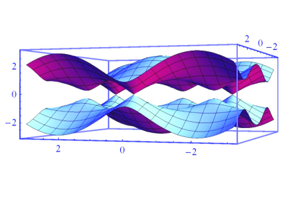
Figure 1: (Color online) The dispersion of electrons for $t^{\prime}=0.0288t$ when $U=0.$ We can see clearly that in the high symmetry point the energy gap is zero and like a Dirac cone.

Let’s explain the quantum phase transitions for different regions of $t^{\prime}$. For $t^{\prime}>0.0288t,$ the quantum phase transition between a QAH and AF SDW order is always second order. Thus when we raise the interaction strength $U,$ due to the smoothly increasing of the staggered magnetization, the QAH state will turn into the A-TSDW after crossing a magnetic phase transition, then turn into the B-TSDW crossing a topological quantum phase transition, eventually turn into the trivial AF SDW state crossing another topological quantum phase transition. However, in the region of $t^{\prime}<0.0288t,$ the quantum phase transition between a BI and AF SDW order is first order which is denoted by the black line in FIG.7 in Ref.he2 . Due to the jumping of the staggered magnetization, the BI state will turn into B-TSDW directly and eventually turn into the trivial AF SDW state crossing a topological quantum phase transition. In the limit $t^{\prime}\rightarrow 0$, the BI state will change into the trivial AF SDW state directly and there is no topological state at all. For the case of $t^{\prime}=0.0288t,$ it is a semi-metal for the weak coupling limit $\left(U/t<2.5\right)$ without electron gap. When we raise the interaction strength $U,$ due to the smoothly increasing of the staggered magnetization, the semi-metal state will turn into the B-TSDW after crossing a magnetic phase transition, eventually turn into the trivial AF SDW state crossing a topological quantum phase transition.

III Effective $\mathrm{NL}\sigma\mathrm{M}$ for magnetic states

For the topological Hubbard model on honeycomb lattice, there are three different magnetic states, A-TSDW, B-TSDW, and trivial AF SDW. A question here is whether these three SDWs with $M\neq 0$ are real long range AF order. The non-zero value of $M$ by mean field method only means the existence of effective spin moments. It does not necessarily imply that the ground state is a long range AF order because the direction of the spins is chosen to be fixed along $\mathbf{\hat{z}}$-axis in the mean field theory. Thus we will examine the stability of magnetic order against quantum spin fluctuations of effective spin moments based on a formulation by keeping spin rotation symmetry, $\sigma_{z}\rightarrow\mathbf{\Omega}\cdot\mathbf{\sigma.}$

By replacing the electronic operators $\hat{c}_{i}^{\dagger}$ and $\hat{c}_{j}$ by Grassmann variables $c_{i}^{\ast}$ and $c_{j}$, in the magnetic state, we get the effective Lagrangian with spin rotation symmetry as

$$\mathcal{L}_{\mathrm{eff}} =\sum_{i,\sigma}c_{i\sigma}^{\ast}\partial_{\tau}c_{i\sigma}-t\sum\limits_{\left\langle{i,j}\right\rangle,\sigma}\left(c_{i\sigma}^{\ast}c_{j\sigma}+h.c.\right)$$

$$-t^{\prime}\sum\limits_{\left\langle\left\langle{i,j}\right\rangle\right\rangle,\sigma}e^{i\phi_{ij}}c_{i\sigma}^{\ast}c_{j\sigma}-\sum_{i}\left(-1\right)^{i}\Delta_{M}c_{i\sigma}^{\ast}\mathbf{\Omega}_{i}\mathbf{\cdot\sigma}c_{i\sigma}$$

$$+\varepsilon\sum\limits_{i\in{A,}\sigma}c_{i\sigma}^{\ast}c_{i\sigma}-\varepsilon\sum\limits_{i\in{B,}\sigma}c_{i\sigma}^{\ast}c_{i\sigma}.$$ (2)

Where $\Delta_{M}=UM/2$, Within the Haldane’s mapping, the spins are parametrized as $\mathbf{\Omega}_{i}=(-1)^{i}\mathbf{n}_{i}\sqrt{1-\mathbf{L}_{i}^{2}}+\mathbf{L}_{i}$Haldane1 ; Auerbach ; dup ; dupuis ; Schulz ; weng . Here $\mathbf{n}_{i}$ is the Néer vector and $\left|\mathbf{n}_{i}\right|=1$, $\mathbf{L}_{i}$ is the transverse canting field, which is chosen to $\mathbf{L}_{i}\cdot\mathbf{n}_{i}=0.$

Then we integrate fermions and the transverse canting field and obtain the effective $\mathrm{NL}\sigma\mathrm{M}$ as

$$\mathcal{L}_{\mathbf{n}}=\frac{1}{2g}[\frac{1}{c}\left(\partial_{\tau}\mathbf{n}\right)^{2}+c\left(\mathbf{\bigtriangledown n}\right)^{2}]\text{ }$$ (3)

with a constraint $\mathbf{n}^{2}=1.$ The coupling constant $g$ and spin wave velocity $c$ are defined as

$$g=\frac{c}{\rho_{s}},\text{ }c^{2}=\frac{\rho_{s}}{\chi^{\perp}}.$$ (4)

Here $\rho_{s}$ is the spin stiffness and $\chi^{\perp}$ is the transverse spin susceptibility. The detailed calculations are given in Appendix. A.

Figure 2: The illustration of the relationship between AF order and quantum disordered state

The properties of the effective $\mathrm{NL}\sigma\mathrm{M}$ are determined by the dimensionless coupling constant $\alpha=g\Lambda.$ The cutoff is defined as the following equation $\Lambda=\min(1,\Delta E/c).$ Here $\Delta E$ is the energy gap of electrons. In particular, there exists a critical point $\alpha_{c}=4\pi$ (or $g_{c}=\frac{4\pi}{\Lambda}$). See illustration of FIG.2. The quantum critical point (QCP) separates the long range spin order from the short range spin order (the quantum disordered state). The dotted line shows the renormalized spin stiffness of the long range spin order and the energy scale of spin gap of the quantum disordered state, respectively (see below discussion).

For the case of $\alpha<4\pi,$ we get solutions of the spin condensed $n_{0}$ and spin gap $m_{s}$ at zero temperature:

$$n_{0}=(1-\frac{g}{g_{c}})^{1/2}\text{, }m_{s}=0.$$ (5)

At finite temperature, the solutions become $n_{0}=0$ and $m_{s}=2k_{\mathrm{B}}T\sinh^{-1}[e^{-\frac{2\pi c}{gk_{\mathrm{B}}T}}\sinh(\frac{c\Lambda}{2k_{\mathrm{B}}T})]$. Because the energy scale of the spin gap $m_{s}$ is always much smaller than the temperature, i.e., $m_{s}\ll k_{\mathrm{B}}T$ (or $\omega_{n}$), quantum fluctuations become negligible in a sufficiently long wavelength and low energy regime $\left(m_{s}<\left|c\mathbf{q}\right|<k_{\mathrm{B}}T\right).$ Thus in this region one may only consider the purely static (semiclassical) fluctuations. The effective Lagrangian of the NL$\sigma$M then becomes

$$\mathcal{L}=\frac{\rho_{\mathrm{s,eff}}}{2}\left(\mathbf{\bigtriangledown n}\right)^{2}$$ (6)

where $\rho_{\mathrm{s,eff}}=c\left(\frac{1}{g}-\frac{1}{g_{c}}\right)$ is the renomalized spin stiffness. At zero temperature, the mass gap vanishes which means that long range AF order appears. To describe the long range AF order, we introduce a spin order parameter

$$\mathcal{M}_{0}=\frac{M}{2}n_{0}=\frac{M}{2}(1-\frac{g}{g_{c}})^{1/2}\text{, }m_{s}=0.$$ (7)

The ground state of long range AF ordered phase has a finite spin order parameter. And in this region there are two transverse Goldstone modes, between them the interaction is irrelevant.

For the case of $\alpha>4\pi,$ the interaction between Goldstone modes becomes relevant and at low energy the renormalized coupling constant diverges. Consequently, the spin gap opens and the long range spin order disappears which mean that the ground state may be a quantum disordered state, and we get the effective model of massive spin-1 excitations

$$\mathcal{L}_{\mathbf{s}}=\frac{1}{2g}\left[(\partial_{\mu}\mathbf{n})^{2}+m_{s}^{2}\mathbf{n}^{2}\right]$$ (8)

with the solutions of $n_{0}$ and $m_{s}$ as

$$n_{0}=0\text{, }m_{s}=4\pi c(\frac{1}{g_{c}}-\frac{1}{g}).$$ (9)

Using the CP(1) representation, we have

$$\mathcal{L}_{\mathbf{s}}=\frac{2}{g}\left[|(\partial_{\mu}-ia_{\mu})\mathbf{z}|^{2}+m_{z}^{2}\mathbf{z}^{2}\right]$$ (10)

where $\mathbf{z}$ is a bosonic spinon, $\mathbf{z}=\left(z_{1},\text{ }z_{2}\right)^{T},$ $\mathbf{n}_{i}=\mathbf{\bar{z}}_{i}\mathbf{\sigma z}_{i}\mathbf{,}$ $\mathbf{\bar{z}z=1,}$ $a_{\mu}\equiv-\frac{i}{2}(\mathbf{\bar{z}}\partial_{\mu}\mathbf{z}-\partial_{\mu}\mathbf{\bar{z}z})$. Here $a_{\mu}$ is introduced as an assistant gauge field. Specifically the local gauge transformation is $z\rightarrow e^{i\varphi(r,\tau)}z$. $m_{z}$ denotes the mass gap for spinons as $m_{z}=m_{s}/2$.

In addition, after integrating over fermions by using gradient expansion approach we also obtain the Chern-Simons-Hopf (CSH) term asKmat ; he2

$$\mathcal{L}_{CSH}=-i\sum_{I,J}\frac{\mathcal{K}_{IJ}}{4\pi}\varepsilon^{\mu\nu\lambda}a_{\mu}^{I}\partial_{\nu}a_{\lambda}^{J}$$ (11)

where $\mathcal{K}$ is 2-by-2 matrix, $a_{\mu}^{I=1}=A_{\mu}$ and $a_{\mu}^{I=2}=a_{\mu}.$ $A_{\mu}$ is the electric-magnetic field. The ”charge” of $A_{\mu}$ and $a_{\mu}$ are defined by $q$ and $q_{s}$, respectively. Thus for different SDW orders with the same order parameter $M$, we have different $\mathcal{K}$-matrices : for A-TSDW order, $\mathcal{K}=\left(\begin{array}[c]{ll}2&0\\ 0&2\end{array}\right);$ for B -TSDW order, $\mathcal{K}=\left(\begin{array}[c]{ll}1&1\\ 1&1\end{array}\right);$ for trivial SDW order, $\mathcal{K}=0.$ See detailed calculations in Appendix. B.

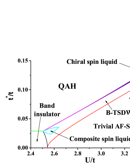
Figure 3: (Color online) The phase diagram: there are seven phases, QAH, band insulator, A-TSDW, B-TSDW, chiral-spin-liquid, composite spin liquid and trivial AF-SDW. The regions of chiral spin liquid and composite spin liquid are the quantum disordered regions of $\alpha>4\pi$.

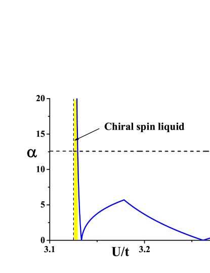
Figure 4: (Color online) The dimensionless coupling constant $\alpha=g\Lambda$ for the case of the parameter as $t^{\prime}=0.1t.$ For the region with $\alpha>4\pi$, the ground state is chiral spin liquid (yellow region).

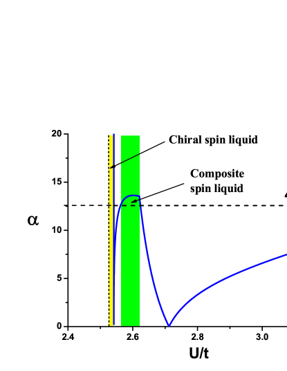
Figure 5: (Color online) The dimensionless coupling constant $\alpha=g\Lambda$ for the case of the parameter as $t^{\prime}=0.033t.$ For the regions with $\alpha>4\pi$, the ground states are spin liquid states - chiral spin liquid (yellow region) or composite spin liquid (green region).

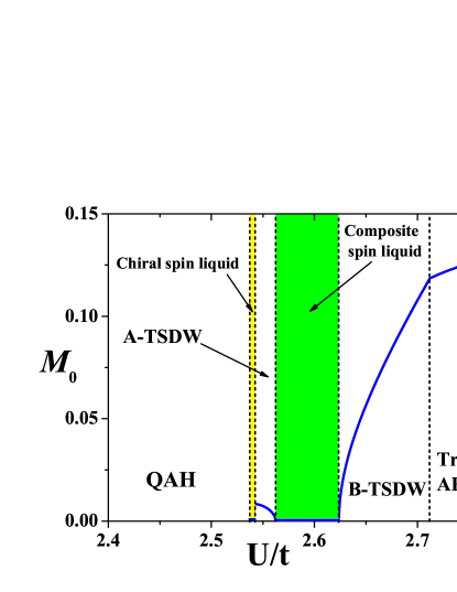
Figure 6: (Color online) The spin order parameter $\mathcal{M}_{0}$ for the case of the parameter as $t^{\prime}=0.033t$. Yellow region denotes chiral spin liquid and green region denotes composite spin liquid, of which $\mathcal{M}_{0}=0$.

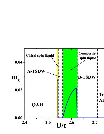
Figure 7: (Color online) The spin gap $m_{s}$ for the case of the parameter as $t^{\prime}=0.033t.$ Yellow region denotes chiral spin liquid and green region denotes composite spin liquid, of which $m_{s}\neq 0$.

Figure 8: (Color online) The dimensionless coupling constant $\alpha=g\Lambda$ for the case of the parameter as $t^{\prime}=0.0288t.$ For the region with $\alpha>4\pi$, the ground state is composite spin liquid (green region).

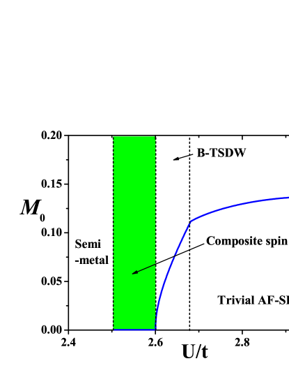
Figure 9: (Color online) The spin order parameter $\mathcal{M}_{0}$ for the case of the parameter as $t^{\prime}=0.0288t$. The green region denotes composite spin liquid, of which $\mathcal{M}_{0}=0$.

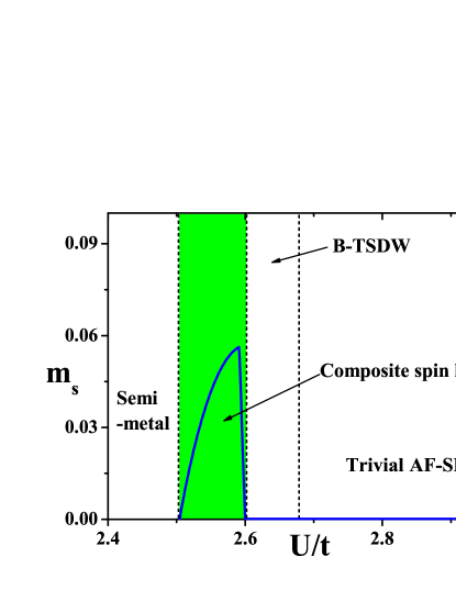
Figure 10: (Color online) The spin gap $m_{s}$ for the case of the parameter as $t^{\prime}=0.0288t.$ The green region denotes composite spin liquid, of which $m_{s}\neq 0$.

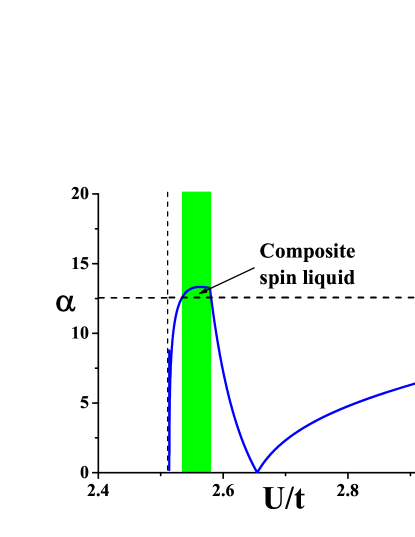
Figure 11: (Color online) The dimensionless coupling constant $\alpha=g\Lambda$ for the case of the parameter as $t^{\prime}=0.025t.$ For the region with $\alpha>4\pi$, the ground state is composite spin liquid (green region).

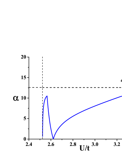
Figure 12: (Color online) The dimensionless coupling constant $\alpha=g\Lambda$ for the case of the parameter as $t^{\prime}=0.02t.$ We can see that the dimensionless coupling constant $\alpha$ is always smaller than $\alpha_{c}=4\pi.$ That mean there doesn’t exist quantum disordered region at all.

For different regions of $t^{\prime},$ we calculated the dimensionless coupling constant $g$ ($\alpha$) and derived the quantum phase transitions between long range AF SDW order and short range one. Thus we can plot a new phase diagram in FIG.3 that shows the quantum disordered regions of $\alpha>4\pi$ (The regions of chiral spin liquid and composite spin liquid).

For a given $t^{\prime}$ bigger than $0.0288t,$ there are two situations. FIG.4 shows the dimensionless coupling constant for one situation with the parameter $t^{\prime}=0.1t$. In FIG.4 there exists a quantum disordered region with $\alpha>\alpha_{c}=4\pi$ in A-TSDW that corresponds to the chiral spin liquid (yellow region). The other case is shown in FIG.5, of which the dimensionless coupling constant for the parameter $t^{\prime}=0.033t$. There are two quantum disordered regions with $\alpha>\alpha_{c}=4\pi$: one corresponds to the chiral spin liquid (yellow region) in A-TSDW, the other is composite spin liquid (green region) in B-TSDW (see discussion in following sections). For this case, we get the energy gap of spin order parameter $\mathcal{M}_{0}$ and spin excitations $m_{s}$ in FIG.6 and FIG.7. One can see that in chiral spin liquid and composite spin liquid, $\mathcal{M}_{0}=0$, $m_{s}\neq 0$. For the case of $t^{\prime}=0.0288t,$ we show the result of the dimensionless coupling constant in FIG.8, from which one can see that there exists a quantum disordered region with $\alpha>\alpha_{c}=4\pi$ in B-TSDW that corresponds to the composite spin liquid (green region). For this case, we also get the energy gap of spin order parameter $\mathcal{M}_{0}$ and spin excitations $m_{s}$ in FIG.9 and FIG.10. One can see that in composite spin liquid, $\mathcal{M}_{0}=0$, $m_{s}\neq 0$. For a given $t^{\prime}$ smaller than $0.0288t,$ there are also two situations. For $0.02377t<t^{\prime}<0.0288t$ $\left(t^{\prime}=0.025t\right),$ from the result shown in FIG.11, we found a quantum disordered region with $\alpha>\alpha_{c}=4\pi$ in B-TSDW that corresponds to the composite spin liquid (green region). For $0<t^{\prime}<0.02377t$ $\left(t^{\prime}=0.02t\right),$ we found that the dimensionless coupling constant $\alpha$ is always smaller than $\alpha_{c}=4\pi.$ That mean there doesn’t exist quantum disordered region at all. We also plot FIG.12 to show this situation.

In the following parts we will use the effective model with CSH terms to learn the properties of different SDW ordershe2 ,

$$\mathcal{L}_{\mathrm{eff}}=\mathcal{L}_{\mathbf{s}}+\mathcal{L}_{CSH}$$

where

$$\mathcal{L}_{\mathbf{s}}=\frac{1}{2g}\left[(\partial_{\mu}\mathbf{n})^{2}+m_{s}^{2}\mathbf{n}^{2}\right]$$

and

$$\mathcal{L}_{CSH}=\sum_{I,J}\frac{K_{IJ}}{4\pi}\varepsilon^{\mu\nu\lambda}a_{\mu}^{I}\partial_{\nu}a_{\lambda}^{J}.$$

Thus an important issue is that what’s the nature of these quantum disordered states with different CSH terms. Our answer is : for the case of A-TSDW with $\mathcal{K}=\left(\begin{array}[c]{ll}2&0\\ 0&2\end{array}\right),$ the quantum disordered state is a chiral spin liquid with topological degeneracy and anyonic excitations (See illustration of FIG.13); for the case of B-TSDW with $\mathcal{K}=\left(\begin{array}[c]{ll}1&1\\ 1&1\end{array}\right),$ the quantum disordered state is composite spin liquid with chiral edge states, of which the elementary excitation is spin one-half charge $\pm e$ objects trapping a topological spin texture (See illustration of FIG.15).

IV Chiral spin liquid - quantum disordered state of A-TSDW

Figure 13: The illustration of the relationship between A-TSDW and chiral spin liquid

Firstly, we study the quantum disordered state of A-TSDW that is described by

$$\mathcal{L}_{\mathrm{eff}} =\frac{1}{2g}\left[(\partial_{\mu}\mathbf{n})^{2}+m_{s}^{2}\mathbf{n}^{2}\right]$$

$$+\frac{1}{2\pi}\epsilon^{\mu\nu\lambda}A_{\mu}\partial_{\nu}A_{\lambda}+\frac{1}{2\pi}\epsilon^{\mu\nu\lambda}a_{\mu}\partial_{\nu}a_{\lambda},$$

or

$$\mathcal{L}_{\mathrm{eff}} =\frac{2}{g}\left[|(\partial_{\mu}-ia_{\mu})\mathbf{z}|^{2}+m_{z}^{2}\mathbf{z}^{2}\right]$$ (12)

$$+\frac{1}{2\pi}\epsilon^{\mu\nu\lambda}A_{\mu}\partial_{\nu}A_{\lambda}+\frac{1}{2\pi}\epsilon^{\mu\nu\lambda}a_{\mu}\partial_{\nu}a_{\lambda}.$$

At low energy limit, the kinetic term of gauge field $a_{\mu}$ is induced

$$\mathcal{L}\left(a_{\mu}\right)=\frac{1}{4e_{a}^{2}}\left(\partial_{\mu}a_{\nu}\right)^{2}.$$ (13)

The induced coupling constant of three dimensional gauge field is $e_{a}^{2}=3\pi m_{z}^{2}$. After considering the CSH term, we have the effective Lagrangian as

$$\mathcal{L}_{\mathrm{eff}} =\frac{1}{4e_{a}^{2}}(\partial_{\mu}a_{\nu})^{2}+\frac{1}{2\pi}\epsilon^{\mu\nu\lambda}a_{\mu}\partial_{\nu}a_{\lambda}$$

$$+\frac{1}{2\pi}\epsilon^{\mu\nu\lambda}A_{\mu}\partial_{\nu}A_{\lambda}.$$ (14)

For the compact U(1) gauge theory in 2+1 dimensions, there exist the instantons (space-time ‘magnetic’ monopoles) that generate $2\pi$ gauge flux of $a_{\mu}$ indicates that $a_{\mu}$ gauge field is ‘compact’confine . Without the CSH term, the monopoles form Coulomb gas in 2+1 dimensions. Due to the Debye screening in the monopole plasma, the gauge field $a_{\mu}$ obtains a mass gap and bosonic spinons $\mathbf{z}$ that couple the gauge field $a_{\mu}$ are confined. And it is pointed out in Ref.wen3 that from the Berry phase of path integral of spin coherent state on honeycomb lattice, the ground state with spinon-confinement is really a VBS state with spontaneous translation symmetry breaking.

However, due to the Chern-Simon term, $\frac{1}{2\pi}\epsilon^{\mu\nu\lambda}a_{\mu}\partial_{\nu}a_{\lambda},$ the instantons are confined by linear potential and irrelevant to low energy physics. Thus the ground state cannot be VBS state and spinons are deconfined. In particular, the Chern-Simons term for $a_{\mu}$ has a nontrivial statistics effect. Because the low energy physics is dominated only by spinon $\mathbf{z}$, due to $\frac{1}{2\pi}\epsilon^{\mu\nu\lambda}a_{\mu}\partial_{\nu}a_{\lambda}$, the statistics angel of $\mathbf{z}$ is $\pi/2$. As a result, spinons $\mathbf{z}$ becomes a semionic particle with spin $J=\frac{1}{4}$! Therefore the quantum disordered state of A-TSDW that is described by the effective Lagrangian in Eq.[12] is really a topological ordered state - chiral spin liquid. From the CSH term, one may derive topological degeneracy - two degenerate ground states of chiral spin liquid on a toruschiral . The result is consistent to that in Ref.he1 .

In addition, one can also derive the edge states from the effective CSH theory. There are two right-moving ”spin” edge excitations described by the following 1D fermion theoryedge

$$\mathcal{L}_{\text{{edge}}}=\sum_{\alpha}\psi_{\alpha s}^{{\dagger}}(\partial_{t}-v_{R}\partial_{x})\psi_{\alpha s},$$

where $\alpha=1,2.$ $\psi_{\alpha s}$ carries a unit of $a_{\mu}$ charge. One can see ”spin” chiral edge states in FIG.14 (the lines with arrows). Correspondingly, one can get the quantized spin Hall conductivity

$$\sigma_{s}=\lim_{\omega\rightarrow 0}{\frac{1}{\omega}}\epsilon_{ij}\left\langle J_{si}(\omega,0)J_{sj}(-\omega,0)\right\rangle=\frac{2e^{2}}{h}.$$ (15)

Here $J_{si}$ denotes spin current, $J_{si}=-i\langle\sum_{a}\bar{\psi}_{a}\gamma_{i}\mathbf{n\cdot\sigma}\psi_{a}\rangle$.

On the other hand, we discuss the properties of $A_{\mu}$. The gauge field $A_{\mu}$ is classical field and has no dynamic terms. Thus the Chern-Simons term for $A_{\mu}$ only indicates quantized anomalous charge Hall effect. From it, we find two right-moving branches of ”charge” edge excitations, which are described by the following one dimension fermion theoryedge0

$$\mathcal{L}_{\text{{edge}}}=\sum_{\alpha}\psi_{c,\alpha}^{{\dagger}}(\partial_{t}-v_{c}\partial_{x})\psi_{c,\alpha},$$ (16)

where $\alpha,\beta=1,2.$ $\psi_{c,\alpha}$ carries a unit of $A_{\mu}$ charge. One can see ”charge” chiral edge state (the lines with dots) in FIG.14. Consequently, we get the quantized charge Hall conductivity $\sigma_{H}=\frac{2e^{2}}{h}.$

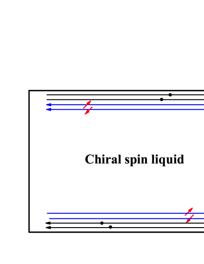
Figure 14: (Color online) The illustration of the edge state of chiral spin liquid. There exist ”spin” chiral edge state (the lines with arrows) and ”charge” chiral edge state (the lines with dots).

Finally, we identify the quantum disordered state of A-TSDW characterized by $g>g_{c}$ to be a chiral spin liquid with quantum anomalous Hall effect (See illustration of FIG.13). For this system, there exists spin-charge separation. In FIG.13, the QCP at $g=g_{c}$ denotes the quantum phase transition dividing long range A-TSDW and short range A-TSDW (chiral SL). In addition, we should emphasis the existence of the chiral spin liquid due to strongly fluctuated spin moments characterized by the diverge behavior of the spin coupling constant near the quantum phase transition (yellow region) in FIG.4 and FIG.5 as $g\rightarrow g_{c}$. Thus the existence of the chiral spin liquid is independent on the cutoff $\Lambda$.

V Composite spin liquid - quantum disordered state of B-TSDW

Figure 15: The illustration of the relationship between B-TSDW and composite spin liquid.

Next we study the quantum disordered state of B-TSDW that is described by the low energy effective Lagrangian

$$\mathcal{L}_{\mathrm{eff}} =\frac{1}{2g}\left[(\partial_{\mu}\mathbf{n})^{2}+m_{s}^{2}\mathbf{n}^{2}\right]+\frac{1}{4\pi}\epsilon^{\mu\nu\lambda}A_{\mu}\partial_{\nu}A_{\lambda}$$

$$+\frac{1}{2\pi}\epsilon^{\mu\nu\lambda}A_{\mu}\partial_{\nu}a_{\lambda}+\frac{1}{4\pi}\epsilon^{\mu\nu\lambda}a_{\mu}\partial_{\nu}a_{\lambda}$$

or

$$\mathcal{L}_{\mathrm{eff}} =\frac{2}{g}\left[|(\partial_{\mu}-ia_{\mu})\mathbf{z}|^{2}+m_{z}^{2}\mathbf{z}^{2}\right]$$

$$+\frac{1}{2\pi}\epsilon^{\mu\nu\lambda}A_{\mu}\partial_{\nu}a_{\lambda}+\frac{1}{4\pi}\epsilon^{\mu\nu\lambda}A_{\mu}\partial_{\nu}A_{\lambda}+\frac{1}{4\pi}\epsilon^{\mu\nu\lambda}a_{\mu}\partial_{\nu}a_{\lambda}.$$

From FIG.15, one can find that there indeed exist a region of short range B-TSDW order that is characterized by $g>g_{c}$.

Figure 16: The illustration of the edge state of composite spin liquid. There exists a single chiral edge mode.

Firstly, we study the statistics of spinon $\mathbf{z}$. To learn the statistics of spinon $\mathbf{z,}$ we can set $A_{\mu}$ to be zero due to $A_{\mu}$ is a classical field. Thus the CS term is reduced into $\frac{1}{4\pi}\epsilon^{\mu\nu\lambda}a_{\mu}\partial_{\nu}a_{\lambda}$. From it we can see that the spinons are fermionic particle by binding a $2\pi$ flux of $a_{\mu}$ that is just a skyrmion (or an anti-skyrmion). On the other hand, due to the mutual Chern-Simons term $\frac{1}{2\pi}\epsilon^{\mu\nu\lambda}A_{\mu}\partial_{\nu}a_{\lambda}$, a $2\pi$ flux of $a_{\mu}$ will carry a electric charge. Thus $\mathbf{z}$ particle is really an ”electron” or a ”hole” binding a skyrmion (or anti-skyrmion). In the following parts we call such composite object ”composite electron (hole)”.

Due to the Chern-Simon term $\frac{1}{4\pi}\epsilon^{\mu\nu\lambda}a_{\mu}\partial_{\nu}a_{\lambda}$, the instantons are also confined by linear potential and irrelevant to low energy physics. Thus the spinons are also deconfined. FIG.17 shows the mass gap of $\mathbf{z}$ particle for the parameter $t^{\prime}=0.033t$, $2m_{z}=4\pi c(\frac{1}{g_{c}}-\frac{1}{g})$. One can see that $m_{z}$ is always much smaller than the mass gap of electrons, $\Delta E$ as $m_{z}\ll\Delta E$. So the low energy physics is dominated by $\mathbf{z}$ particle, the so-called composite electron (hole).

Secondly, we study the properties of gauge fluctuations. After integrating the massive $\mathbf{z}$ particle, the effective Lagrangian for gauge field $a_{\mu}$ becomes

$$\mathcal{L}_{\mathrm{eff}} =\frac{1}{4e_{a}^{2}}(\partial_{\mu}a_{\nu})^{2}+\frac{1}{4\pi}\epsilon^{\mu\nu\lambda}a_{\mu}\partial_{\nu}a_{\lambda}$$

$$+\frac{1}{2\pi}\epsilon^{\mu\nu\lambda}A_{\mu}\partial_{\nu}a_{\lambda}+\frac{1}{4\pi}\epsilon^{\mu\nu\lambda}A_{\mu}\partial_{\nu}A_{\lambda}.$$ (17)

Then the partition function of the effective model is written as

$$\mathcal{Z}=\int\mathcal{D}\left[a\right]e^{-\int_{0}^{\beta}d\tau\mathcal{L}_{\mathrm{eff}}}.$$

Then we introduce $a_{+,\mu}=A_{\mu}+a_{\mu},\ a_{-,\mu}=A_{\mu}-a_{\mu}\$and get the partition function as

$$\mathcal{Z}=\int\mathcal{D}\left[a_{+}\right]e^{-\int_{0}^{\beta}d\tau\mathcal{L}_{\mathrm{eff}}},$$

where

$$\mathcal{L}_{\mathrm{eff}}=\frac{1}{4e_{a}^{2}}(\partial_{\mu}a_{\nu,+})^{2}+\frac{1}{4\pi}\epsilon^{\mu\nu\lambda}a_{\mu,+}\partial_{\nu}a_{\lambda,+}.$$ (18)

With the Chern-Simons term $\frac{1}{4\pi}\epsilon^{\mu\nu\lambda}a_{\mu,+}\partial_{\nu}a_{\lambda,+}$, the gauge field $a_{\mu,+}$ indicates quantized spin-charge synchronized edge states and quantized spin-charge synchronized Hall effect pointed out in Ref.he2 . The edge excitation is described by the following one dimension fermion theoryedge0 ; edge

$$\mathcal{L}_{\text{{edge}}}=\tilde{\psi}^{{\dagger}}(\partial_{t}-\tilde{v}\partial_{x})\tilde{\psi}$$ (19)

where $\tilde{\psi}$ carries a unit of $a_{+,\mu}$ ”charge”. One can see a chiral edge mode (the lines in FIG.16). Consequently, we get the spin-charge synchronized Hall conductivity as

$$\tilde{\sigma}=\lim_{\omega\rightarrow 0}{\frac{1}{\omega}}\epsilon_{ij}\left\langle\tilde{J}_{i}(\omega,0)\tilde{J}_{j}(-\omega,0)\right\rangle=\frac{e^{2}}{h}$$ (20)

where

$$\tilde{J}_{i}=i\langle\sum_{a}\bar{\psi}_{a}\gamma_{i}(1-\mathbf{n\cdot\sigma)}\psi_{a}/2\rangle.$$ (21)

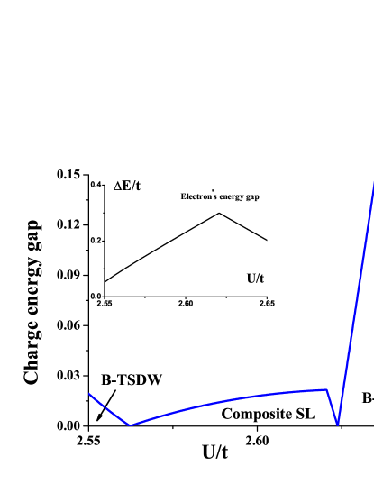
Figure 17: (Color online) The charge energy gap for case of $t^{\prime}=0.033t$, $\varepsilon=0.15t$: the charge carrier is composite electron. In composite SL, the charge energy gap is that of spin gap, $m_{s}$; in B-TSDW, the charge energy gap is that of a pair of skyrmion and anti-skyrmion, $\Delta_{c}$. The energy gap of fermion quasi-particles are very big (see inset).

Finally we use the duality relationship between spinons and skyrmions to learn the quantum phase transition at $g=g_{c}$ dividing long range B-TSDW and short range B-TSDW (composite SL).

In B-TSDW, we can define the skyrmion (or anti-skyrmion) with winding number $\mathcal{Q}=\int\mathbf{d^{2}\mathbf{r}}\frac{1}{4\pi}\epsilon_{0\nu\lambda}\mathbf{n_{\mathrm{s}}\cdot\partial}^{\nu}\mathbf{n_{\mathrm{s}}\times\partial}^{\lambda}\mathbf{n_{\mathrm{s}}=\pm}1,$ of which the solutions in the continuum limit are pol

$$\mathbf{n}_{\mathrm{s}} =(\frac{\lambda(x-x_{0})}{|\mathbf{r}-\mathbf{r}_{0}|^{2}+\lambda^{2}},\text{ }\pm\frac{\lambda(y-y_{0})}{|\mathbf{r}-\mathbf{r}_{0}|^{2}+\lambda^{2}},\text{ }$$ (22)

$$\pm\frac{\lambda}{|\mathbf{r}-\mathbf{r}_{0}|^{2}+\lambda^{2}}).$$

Here $\lambda$ is the radius of the skyrmion at $\mathbf{r}_{0}=(x_{0},y_{0})$. In long range B-TSDW, due to ”spin-charge synchronized charge-flux binding” effect, $Q=\pm 1$ skyrmion carries a unit electric charge $q=\mp 1$ and a unit ”charge” $q_{s}=\mp 1$. With a unit ”charge” $q_{s}$, a $Q=\pm 1$ skyrmion gets half spin and becomes a charged $S=1/2$ fermion.

The mass of the skyrmion (or anti-skyrmion) is associated with

$$m_{\mathrm{skyrmion}}=m_{\mathrm{anti-skyrmion}}=\frac{\rho_{\mathrm{s,eff}}}{2}\int{d^{2}\mathbf{{r}}}\left({\nabla\mathbf{{n}}}_{\mathrm{s}}\right)^{2}=4\pi\rho_{\mathrm{s,eff}}$$

where $\rho_{\mathrm{s,eff}}=(1-\frac{g}{g_{c}})\rho_{\mathrm{s}}$. This result indicates the charge gap is really the mass gap of a pair of skyrmion-anti-skyrmion

$$\Delta_{c}=m_{\mathrm{skyrmion}}+m_{\mathrm{anti-skyrmion}}=8\pi(1-\frac{g}{g_{c}})\rho_{\mathrm{s}}$$ (23)

that will close at the critical point $g=g_{c}$, $\Delta_{c}\rightarrow 0$. From FIG.5, one can see that there exists two QCPs ($g=g_{c}$) between B-TSDW and composite SL, at which the charged excitations have no energy gap, while the usual electrons without trapping spin texture still has big mass gap $\Delta E\gg\Delta_{c}$ (see inset of FIG.17). In B-TSDW, the low energy charge dynamics is dominated by fermionic charged skyrmions rather than the electrons. At these QCPs, the system is a semi-metal with gapless charge excitations. The dotted line in FIG.15 is the energy scale of the charge gap.

Finally we find that there exists a new type of spin liquid - composite spin liquid. The low energy excitations are ”composite electrons” that are $S=1/2$ charge $\pm e$ fermions with trapping a topological spin texture. See illustration in FIG.18. At the QCPs between long range B-TSDW and composite SL, the system becomes a semi-metal with gapless charge excitations (even for gapped electrons).

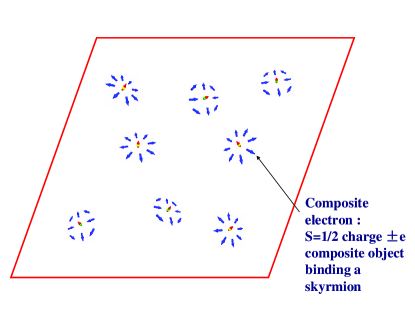
Figure 18: (Color online) The illustration of composite spin liquid, of which the elementary excitations are the ”composite electrons” that are $S=1/2$ charge $\pm e$ fermions with trapping a topological spin texture.

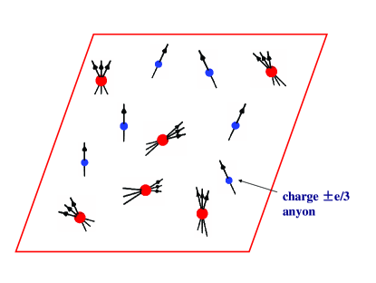
Figure 19: (Color online) The illustration of Fractional quantum Hall state. Small blue balls with single arrow denotes the anyonic excitations with $\pm e/3$ charge.

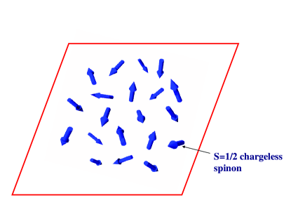
Figure 20: (Color online) The illustration of quantum spin liquid. The blue arrows denote an $S=1/2$ chargeless spinons.

VI Conclusion and discussion

In the end, we give a summary. We found a new type of topological state which we name as composite spin liquid. Composite spin liquid state can be regarded as a short range B-type topological spin-density-wave which is beyond the classification of traditional spin liquid states. For traditional spin liquid states, there always exists spin-charge separation. While for composite spin liquid there is no spin-charge separation. Instead, the elementary excitations are ”composite electrons” with both spin degree of freedom and charge degree of freedom, together with topological spin texture. This topological state supports single chiral edge mode but no topological degeneracy. In addition, the QCPs between long range B-TSDW and composite SL are also nontrivial, at which the system becomes a semi-metal with gapless charge excitations (even for gapped electrons).

In addition, we give a comparison on different exotic quantum orders beyond Landau’s theory:

	Excitations	Topological degeneracy	Edge state	Classification
FQH state	Charged anyon	Yes	Yes	K-matrix
TBI	Electron	No	Yes	Ten-fold way
SL	Spinon	–	–	PSG
Composite SL	Composite electron	No	Yes	?

Table 1: The differences (the types of excitations, if there exists topological degeneracy for the ground states on torus, if there exist edge states, the way to classify the topological states) between four exotic quantum orders beyond Landau’s theory: fractional quantum Hall state(FQH), topological band insulator (TBI), spin liquid (SL), composite spin liquid (SL).

1. Fractional quantum Hall (FQH) state : due to charge-flux binding effect, the elementary excitations are anyonic excitations with fractional electric charge and fractional quantized Hall conductivityTSG8259 ; Laughlinc . FIG.19 shows the anyonic excitations with $\pm e/3$ charge (small blue balls with single arrow). The ground state on a torus has topological degeneracy. For the open system, there exist chiral edge states on its boundary. By their effective CS theories (or K-matrix theoryKmat ; read ; fr ), people can classify fractional quantized Hall states into different Abelian states and nonAbelian states;

2. Topological band insulator (TBI) : the elementary excitations are gapped electrons (or holes). For this topological state, there exist gapless edge states. However, there is no topological degeneracy for the ground state. By ”ten-fold way” of random matrix, people classify topological band insulators into $Z_{2}$ type or $Z$ typezi ; ki ; ry ;

3. Spin liquid (SL) : due to the big electron gap (Mott gap), the excitations are deconfined spinons with only spin degree of freedom. In FIG.20, the blue arrow denotes an $S=1/2$ chargeless spinon. By PSGs, people classify quantum spin liquid states into $SU(2)$ type, $U(1)$ type or $Z_{2}$ typewen ; wxg . For topological spin liquid (for example chiral spin liquid), there exist gapless edge states and topological degeneracy; while for gapless spin liquid (for example algebraic spin liquid), there is no well defined gapless edge states and topological degeneracy. For this reason we use ”$-$” to denote the uncertainty in table.1;

4. Composite spin liquid : the elementary excitations are the ”composite electrons” with both spin degree of freedom and charge degree of freedom, together with topological spin texture (See FIG.18). For this topological states, there exist gapless edge states but no topological degeneracy. Till now we don’t know how to characterize composite spin liquid states. For this reason we use ”$?$” to denote the situation in table.1.

Finally, we address the relevant experimental realization. This topological Hubbard model on honeycomb lattice may be simulated in optical lattice of cold atoms. In Ref.zhu , it is proposed that the (spinless) Haldane model on honeycomb optical lattice can be realized in the cold atoms. When two-component fermions with repulsive interaction are put into such optical lattice, one can get an effective topological Hubbard model. It is easy to change the potential barrier by varying the laser intensities to tune the Hamiltonian parameters including the hopping strength ($t$-term), the staggered potential ($\varepsilon$-term) and the particle interaction ($U$-term).

VII Appendix A: Theory of spin fluctuations - to get the O(3) nonlinear $\sigma$ model

The Hamiltonian of the topological Hubbard model on honeycomb lattice is given by

$$H =-t\sum\limits_{\left\langle{i,j}\right\rangle,\sigma}\left(\hat{c}_{i\sigma}^{\dagger}\hat{c}_{j\sigma}+h.c.\right)-t^{\prime}\sum\limits_{\left\langle\left\langle{i,j}\right\rangle\right\rangle,\sigma}e^{i\phi_{ij}}\hat{c}_{i\sigma}^{\dagger}\hat{c}_{j\sigma}$$

$$+U\sum\limits_{i}\hat{n}_{i\uparrow}\hat{n}_{i\downarrow}+\mu\sum\limits_{i,\sigma}\hat{c}_{i\sigma}^{\dagger}\hat{c}_{i\sigma}$$

$$+\varepsilon\sum\limits_{i\in{A,}\sigma}\hat{c}_{i\sigma}^{\dagger}\hat{c}_{i\sigma}-\varepsilon\sum\limits_{i\in{B,}\sigma}\hat{c}_{i\sigma}^{\dagger}\hat{c}_{i\sigma}.$$ (24)

$t$ and $t^{\prime}$ are the nearest neighbor and the next nearest neighbor hoppings, respectively. We introduce a complex phase $\phi_{ij}$ $\left(\left|\phi_{ij}\right|=\frac{\pi}{2}\right)$ to the next nearest neighbor hopping, of which the positive phase is set to be clockwise. $U$ is the on-site Coulomb repulsion. $\sigma$ are the spin-indices representing spin-up $(\sigma=\uparrow)$ and spin-down $(\sigma=\downarrow)$ for electrons, $\varepsilon$ denotes an on-site staggered energy and is set to be $0.15t$. .

For free fermions (the on-site Coulomb repulsion $U$ is zero), the spectrum

$$E_{\mathbf{k}}=\sqrt{\left|\xi_{k}\right|^{2}+\left(\xi_{k}^{\prime}+\varepsilon\right)^{2}}$$ (25)

where

$$\left|\xi_{\mathbf{k}}\right|=t\sqrt{3+2\cos{(\sqrt{3}k_{y})}+4\cos{(3k_{x}/2)}\cos{(\sqrt{3}k_{y}/2)}}$$

and

$$\xi_{k}^{\prime}=2t^{\prime}\sum\limits_{i}\sin{(\mathbf{k}\cdot\mathbf{b}_{i})}.$$ (26)

Where ${\mathbf{b}_{i}}$ is the nest nearest vectors. According to this spectrum $E_{\mathbf{k}}$, we can see that there exist energy gaps $\Delta_{f1}$, $\Delta_{f2}$ near points $\mathbf{k}_{1}=-\frac{2\pi}{3}(1,$ $1/\sqrt{3})$ and $\mathbf{k}_{2}=\frac{2\pi}{3}(1,$ $1/\sqrt{3})$ as $\Delta_{f1}=\left|2\varepsilon-6\sqrt{3}t^{\prime}\right|$ and $\Delta_{f2}=2\varepsilon+6\sqrt{3}t^{\prime},$ respectively. There exist two phases separated by the phase boundary $2\varepsilon=6\sqrt{3}t^{\prime}$, the quantum anomalous Hall (QAH) state and the normal band insulator (BI) state with trivial topological properties.

Because the Hubbard model on bipartite lattices is unstable against antiferromagnetic instability, at half-filling, the ground state may be an insulator with AF-SDW order with increasing interacting strength. Such AF-SDW order is described by the following mean field order parameter $\langle(-1)^{i}\hat{c}_{i}^{{\dagger}}\sigma^{z}\hat{c}_{i}\rangle=M.$ Here $M$ is the staggered magnetization. In the mean field theory, the Hamiltonian of the topological Hubbard model is obtained as

$$H_{MF}=H-\sum\limits_{i}(-1)^{i}\Delta_{M}\hat{c}_{i}^{\dagger}\sigma_{z}\hat{c}_{i}$$ (27)

where $\Delta_{M}=\frac{UM}{2}$. Then in the momentum space we get

$$H=\sum_{k}c_{k}^{\dagger}h_{k}c_{k},$$ (28)

where $c_{k}^{\dagger}=(c_{k,A\uparrow}^{\dagger},c_{k,A\downarrow}^{\dagger},c_{k,B\uparrow}^{\dagger},c_{k,B\downarrow}^{\dagger})$ and

$$h_{k}=\left(\begin{array}[c]{cc}\xi_{\mathbf{k}^{\prime}}+\frac{UM}{2}\sigma_{z}+\varepsilon&\xi_{\mathbf{k}}\\ \left(\xi_{\mathbf{k}}\right)^{\ast}&-\xi_{\mathbf{k}^{\prime}}-\frac{UM}{2}\sigma_{z}-\varepsilon\end{array}\right).$$

After diagonalization, we can get the quasi-particles spectrums

$$E_{\mathbf{k}_{1}}=\pm\sqrt{(\xi_{k}^{\prime}+\Delta_{M}+\varepsilon)^{2}+|\xi_{k}|^{2}}$$ (29)

and

$$E_{\mathbf{k}_{2}}=\pm\sqrt{(\xi_{k}^{\prime}-\Delta_{M}+\varepsilon)^{2}+|\xi_{k}|^{2}}.$$ (30)

By minimizing the ground state’s energy, the self-consistent equation in the reduced BZ is reduced into

$$1=\frac{1}{N_{s}M}\sum\limits_{\mathbf{k\in}BZ}{[\frac{\xi_{\mathbf{k}}^{\prime}+\Delta_{M}+\varepsilon}{2E_{\mathbf{k}_{1}}}-\frac{\xi_{\mathbf{k}}^{\prime}-\Delta_{M}+\varepsilon}{2E_{\mathbf{k}_{2}}}{]}}$$ (31)

where $N_{s}$ is the number of unit cells. The phase diagram has been obtained in Ref.he2 . There are totally five phases, NI state, QAH state, A-TSDW state, B-TSDW state and trivial AF-SDW state seperated by two types of phase transitions : one is the magnetic phase transition [denoted by $(U/t)_{M}$] between a magnetic order state with $M\neq 0$ and a non-magnetic state with $M=0$, the other one is the topological quantum phase transition [denoted by $(\frac{U}{t})_{c1}$ or $(\frac{U}{t})_{c2}$] that is characterized by the condition of zero fermion’s energy gaps, $\Delta_{f1}=-6\sqrt{3}t^{\prime}+2\varepsilon+UM=0$ or $\Delta_{f2}=6\sqrt{3}t^{\prime}+2\varepsilon-UM=0$.

We deal with the spin fluctuations by using the path-integral formulation of electrons with spin rotation symmetry. The interaction term can be handled by using the SU(2) invariant Hubbard-Stratonovich decomposition in the arbitrary on-site unit vector $\mathbf{\Omega}_{i}$

$$\hat{n}_{i\uparrow}\hat{n}_{i\downarrow}=\frac{\left(\hat{c}_{i}^{\dagger}\hat{c}_{i}\right)^{2}}{4}-\frac{1}{4}[\mathbf{\Omega}_{i}\mathbf{\cdot}\hat{c}_{i}^{{\dagger}}\mathbf{\sigma}\hat{c}_{i}]^{2}.$$ (32)

Here $\mathbf{\sigma=}\left(\sigma_{x},\sigma_{y},\sigma_{z}\right)$ are the Pauli matrices. By replacing the electronic operators $\hat{c}_{i}^{\dagger}$ and $\hat{c}_{j}$ by Grassmann variables $c_{i}^{\ast}$ and $c_{j}$, the effective Lagrangian of the 2D generalized Hubbard model at half filling is obtained:

$$\mathcal{L}_{\mathrm{eff}} =\sum_{i,\sigma}c_{i\sigma}^{\ast}\partial_{\tau}c_{i,\sigma}-t\sum\limits_{\left\langle{i,j}\right\rangle,\sigma}\left(c_{i\sigma}^{\ast}c_{j\sigma}+h.c.\right)$$

$$-t^{\prime}\sum\limits_{\left\langle\left\langle{i,j}\right\rangle\right\rangle,\sigma}e^{i\phi_{ij}}c_{i\sigma}^{\ast}c_{j\sigma}-\Delta_{M}\sum_{i{,\sigma}}c_{i{,\sigma}}^{\ast}\mathbf{\Omega}_{i}\mathbf{\cdot\sigma}c_{i{,\sigma}}$$

$$+\varepsilon\sum\limits_{i\in{A,\sigma}}c_{i\sigma}^{\ast}c_{i\sigma}-\varepsilon\sum\limits_{i\in{B,\sigma}}c_{i\sigma}^{\ast}c_{i\sigma}.$$ (33)

To describe the spin fluctuations, we use the Haldane’s mapping:

$$\mathbf{\Omega}_{i}=(-1)^{i}\mathbf{n}_{i}\sqrt{1-\mathbf{L}_{i}^{2}}+\mathbf{L}_{i}$$ (34)

where $\mathbf{n}_{i}=(n_{i}^{x},n_{i}^{y},n_{i}^{z})$ is the Neel vector that corresponds to the long-wavelength part of $\mathbf{\Omega}_{i}$ with a restriction $\mathbf{n}_{i}^{2}=1.$ $\mathbf{L}_{i}$ is the transverse canting field that corresponds to the short-wavelength parts of $\mathbf{\Omega}_{i}$ with a restriction $\mathbf{L}_{i}\cdot\mathbf{n}_{i}=0$. We then rotate $\mathbf{\Omega}_{i}$ to $\mathbf{\hat{z}}$-axis for the spin indices of the electrons at $i$-site:

$$\psi_{i} =U_{i}^{\dagger}c_{i}$$ (35)

$$U_{i}^{\dagger}\mathbf{n}_{i}\cdot\mathbf{\sigma}U_{i} =\mathbf{\sigma}_{z}$$ (36)

$$U_{i}^{\dagger}\mathbf{L}_{i}\cdot\mathbf{\sigma}U_{i} =\mathbf{l}_{i}\cdot\mathbf{\sigma}$$ (37)

where $U_{i}\in$SU(2)/U(1).

One then can derive the following effective Lagrangian after such spin transformation:

$$\mathcal{L}_{\mathrm{eff}} =\sum\limits_{i,\sigma}\psi_{i,\sigma}^{\ast}\partial_{\tau}\psi_{i,\sigma}+\sum_{i,\sigma}\psi_{i,\sigma}^{\ast}a_{0}\left(i\right)\psi_{i,\sigma}$$

$$-t\sum\limits_{\left\langle{i,j}\right\rangle,\sigma}\left(\psi_{i,\sigma}^{\ast}e^{ia_{ij}}\psi_{j,\sigma}+h.c.\right)-t^{\prime}\sum\limits_{\left\langle\left\langle{i,j}\right\rangle\right\rangle,\sigma}e^{i\phi_{ij}}\psi_{i,\sigma}^{\ast}e^{ia_{ij}}\psi_{j,\sigma}$$

$$+\varepsilon\sum\limits_{i\in{A,\sigma}}\psi_{i,\sigma}^{\ast}e^{ia_{ii}}\psi_{i,\sigma}-\varepsilon\sum\limits_{i\in{B,\sigma}}\psi_{i,\sigma}^{\ast}e^{ia_{ii}}\psi_{i,\sigma}$$

$$-\Delta_{M}\sum_{i{,\sigma}}\psi_{i,\sigma}^{\ast}\left[\left(-1\right)^{i}\mathbf{\sigma}_{z}\sqrt{1-\mathbf{l}_{i}^{2}}+\mathbf{l}_{i}\cdot\mathbf{\sigma}\right]\psi_{i,\sigma}$$ (38)

where the auxiliary gauge fields $a_{ij}=a_{ij,1}\sigma_{x}+a_{ij,2}\sigma_{y}$ and $a_{0}\left(i\right)=a_{0,1}\left(i\right)\sigma_{x}+a_{0,2}\left(i\right)\sigma_{y}\$are defined as

$$e^{ia_{ij}}=U_{i}^{\dagger}U_{j},\text{ }a_{0}\left(i\right)=U_{i}^{\dagger}\partial_{\tau}U_{i}.$$ (39)

In terms of the mean field result $M=\left(-1\right)^{i}\langle\psi_{i}^{\ast}\mathbf{\sigma}_{z}\psi_{i}\rangle$ as well as the approximations,

$$\sqrt{1-\mathbf{l}_{i}^{2}}\simeq 1-\frac{\mathbf{l}_{i}^{2}}{2},\text{ }e^{ia_{ij}}\simeq 1+ia_{ij},$$

we obtain the effective Hamiltonian as:

$$\mathcal{L}_{\mathrm{eff}} \simeq\sum\limits_{i,\sigma}\psi_{i,\sigma}^{\ast}\partial_{\tau}\psi_{i,\sigma}+\sum_{i,\sigma}\psi_{i,\sigma}^{\ast}\left(a_{0}\left(i\right)-\Delta\mathbf{l}_{i}\cdot\mathbf{\sigma}\right)\psi_{i,\sigma}$$

$$-\Delta_{M}\sum_{i{,\sigma}}\left(-1\right)^{i}\psi_{i,\sigma}^{\ast}\mathbf{\sigma}_{z}\psi_{i,\sigma}-t\sum\limits_{\left\langle{i,j}\right\rangle,\sigma}\psi_{i,\sigma}^{\ast}\left(1+ia_{ij}\right)\psi_{j,\sigma}$$

$$-t^{\prime}\sum\limits_{\left\langle\left\langle{i,j}\right\rangle\right\rangle,\sigma}e^{i\phi_{ij}}\psi_{i,\sigma}^{\ast}\left(1+ia_{ij}\right)\psi_{j,\sigma}+\Delta M\sum_{i{,\sigma}}\frac{\mathbf{l}_{i}^{2}}{2}$$

$$+\varepsilon\sum\limits_{i\in{A,\sigma}}\psi_{i,\sigma}^{\ast}\left(1+ia_{ii}\right)\psi_{i,\sigma}-\varepsilon\sum\limits_{i\in{B,\sigma}}\psi_{i,\sigma}^{\ast}\left(1+ia_{ii}\right)\psi_{i,\sigma}$$ (40)

By integrating out the fermion fields $\psi_{i}^{\ast}$ and $\psi_{i},$ the effective action with the quadric terms of $[a_{0}\left(i\right)-\Delta\mathbf{\sigma\cdot l}_{i}]$ and $a_{ij}$ becomes

$$\mathcal{S}_{\mathrm{eff}}=\frac{1}{2}\int_{0}^{\beta}d\tau\sum_{i}[-4\varsigma(a_{0}\left(i\right)-\Delta_{M}\mathbf{\sigma\cdot l}_{i})^{2}+4\rho_{s}a_{ij}^{2}+\frac{2\Delta_{M}^{2}}{U}\mathbf{l}_{i}^{2}].$$ (41)

To give $\rho_{s}$ and $\varsigma$ for calculation in detail, we choose $U_{i}$ to be

$$U_{i}=(\begin{array}[c]{cc}z_{i\uparrow}^{\ast}&z_{i\downarrow}^{\ast}\\ -z_{i\downarrow}&z_{i\uparrow}\end{array}),$$ (42)

where $\mathbf{n}_{i}=\mathbf{\bar{z}}_{i}\mathbf{\sigma z}_{i},$ $\mathbf{z}_{i}=\left(z_{i\uparrow},z_{i\downarrow}\right)^{T},$ $\mathbf{\bar{z}}_{i}\mathbf{z}_{i}\mathbf{=1.}$ And the spin fluctuations around $\mathbf{n}_{i}=\mathbf{\hat{z}}_{i}$ is

$$\mathbf{n}_{i} =\mathbf{\hat{z}}_{i}\mathbf{+}\text{Re}\left(\mathbf{\phi}_{i}\right)\mathbf{\hat{x}+}\text{Im}\left(\mathbf{\phi}_{i}\right)\mathbf{\hat{y}}$$ (43)

$$\mathbf{z}_{i} =\left(\begin{array}[c]{c}1-\left|\mathbf{\phi}_{i}\right|^{2}/8\\ \mathbf{\phi}_{i}/2\end{array}\right)+O(\mathbf{\phi}_{i}^{3}).$$ (46)

Then the quantities $U_{i}^{\dagger}U_{j}$ and $U_{i}^{\dagger}\partial_{\tau}U_{i}$ can be expanded in the power of $\mathbf{\phi}_{i}-\mathbf{\phi}_{j}$ and $\partial_{\tau}\mathbf{\phi}_{i},$

$$U_{i}^{\dagger}U_{j} =e^{-i\frac{\mathbf{\phi}_{i}-\mathbf{\phi}_{j}}{2}\sigma_{y}}$$ (47)

$$U_{i}^{\dagger}\partial_{\tau}U_{i} =\left(\begin{array}[c]{cc}0&\frac{1}{2}\partial_{\tau}\mathbf{\phi}_{i}\\ -\frac{1}{2}\partial_{\tau}\mathbf{\phi}_{i}&0\end{array}\right).$$ (50)

According to Eq.(39), the gauge field $a_{ij}$ and $a_{0}\left(i\right)$ are given as

$$a_{ij} =-\frac{1}{2}\left(\mathbf{\phi}_{i}-\mathbf{\phi}_{j}\right)\mathbf{\sigma}_{y}$$ (51)

$$a_{0}\left(i\right) =\frac{i}{2}\partial_{\tau}\mathbf{\phi}_{i}\mathbf{\sigma}_{y}.$$ (52)

Supposing $a_{ij}$ and $a_{0}\left(i\right)$ to be a constant in space and denoting $\mathbf{\partial}_{i}\mathbf{\mathbf{\phi}}_{i}\mathbf{=a}$ and $\partial_{\tau}\mathbf{\phi}_{i}=iB_{y}$, we have

$$a_{ij} =-\frac{1}{2}\mathbf{a\cdot(i-j)\sigma}_{y}$$ (53)

$$a_{0}\left(i\right) =-\frac{1}{2}B_{y}\mathbf{\sigma}_{y}.$$ (54)

The energy of Hamiltonian of Eq.(41) becomes

$$E\left(B_{y},\mathbf{a}\right)=-\frac{1}{2}\zeta B_{y}^{2}+\frac{1}{2}\rho_{s}\mathbf{a}^{2}.$$ (55)

Then one could get $\zeta$ and $\rho_{s}$ from the following equations by calculating the partial derivative of the energy

$$\zeta =-\frac{1}{N}\frac{\partial^{2}E_{0}\left(B_{y}\right)}{\partial B_{y}^{2}}|_{B_{y}=0}$$ (56)

$$\rho_{s} =\frac{1}{N}\frac{\partial^{2}E_{0}\left(\mathbf{a}\right)}{\partial\mathbf{a}^{2}}|_{\mathbf{a}=0}.$$ (57)

Here $E_{0}\left(B_{y}\right)$ and $E_{0}\left(\mathbf{a}\right)$ are the energy of the lower Hubbard band

$$E_{0}\left(B_{y}\right) =\sum\limits_{\mathbf{k}}\left(E_{+,\mathbf{k}}^{\zeta}+E_{-,\mathbf{k}}^{\zeta}\right)$$ (58)

$$E_{0}\left(\mathbf{a}\right) =\sum\limits_{\mathbf{k}}\left(E_{+,\mathbf{k}}^{\rho}+E_{-,\mathbf{k}}^{\rho}\right)$$ (59)

where $E_{+,\mathbf{k}}^{\zeta},$ $E_{-,\mathbf{k}}^{\zeta}$ and $E_{+,\mathbf{k}}^{\rho},$ $E_{-,\mathbf{k}}^{\rho}$ are the energies of the following Hamiltonian $\mathcal{H}^{\zeta}$ and $\mathcal{H}^{\rho}$

$$\mathcal{H}^{\zeta} =-t\sum\limits_{\left\langle{i,j}\right\rangle,\sigma}\left(\psi_{i,\sigma}^{\ast}\psi_{j,\sigma}+h.c.\right)-t^{\prime}\sum\limits_{\left\langle\left\langle{i,j}\right\rangle\right\rangle,\sigma}e^{i\phi_{ij}}\psi_{i,\sigma}^{\ast}\psi_{j,\sigma}$$

$$+\varepsilon\sum\limits_{i\in{A,\sigma}}\psi_{i,\sigma}^{\ast}\psi_{i,\sigma}-\varepsilon\sum\limits_{i\in{B,\sigma}}\psi_{i,\sigma}^{\ast}\psi_{i,\sigma}$$

$$+\sum_{i,\sigma}\psi_{i,\sigma}^{\ast}a_{0}\left(i\right)\psi_{i,\sigma}-\Delta_{M}\sum_{i{,\sigma}}\left(-1\right)^{i}\psi_{i,\sigma}^{\ast}\mathbf{\sigma}_{z}\psi_{i,\sigma},$$ (60)

$$\mathcal{H}^{\rho} =-t\sum\limits_{\left\langle{i,j}\right\rangle,\sigma}\psi_{i,\sigma}^{\ast}e^{ia_{ij}}\psi_{j,\sigma}-t^{\prime}\sum\limits_{\left\langle\left\langle{i,j}\right\rangle\right\rangle,\sigma}e^{i\phi_{ij}}\psi_{i,\sigma}^{\ast}e^{ia_{ij}}\psi_{j,\sigma}$$

$$+\varepsilon\sum\limits_{i\in{A,\sigma}}\psi_{i,\sigma}^{\ast}e^{ia_{ii}}\psi_{i,\sigma}-\varepsilon\sum\limits_{i\in{B,\sigma}}\psi_{i,\sigma}^{\ast}e^{ia_{ii}}\psi_{i,\sigma}$$

$$-\Delta_{M}\sum_{i{,\sigma}}\left(-1\right)^{i}\psi_{i,\sigma}^{\ast}\mathbf{\sigma}_{z}\psi_{i,\sigma}$$ (61)

Using the Fourier transformation for $\mathcal{H}^{\zeta}$, we have the spectrum of the lower band of $\mathcal{H}^{\zeta}$:

$$E_{\pm,\mathbf{k}}^{{}^{\zeta}}=-\frac{1}{2}\sqrt{4|\xi_{k}|^{2}+2a^{2}+B_{y}^{2}+2d^{2}\pm 2\sqrt{a^{4}+B_{y}^{2}a^{2}-2a^{2}d^{2}+B_{y}^{2}d^{2}+4B_{y}^{2}|\xi_{k}|^{2}+d^{4}+2adB_{y}^{2}}}$$ (62)

where $a=\xi_{k^{\prime}}+\frac{UM}{2}+\varepsilon$ and $d=\xi_{k^{\prime}}-\frac{UM}{2}+\varepsilon$.

Using $\varsigma=-\frac{1}{N}\frac{\partial^{2}E_{0}{(B_{y})}}{\partial B_{y}^{2}}|_{B_{y}=0}$ and $E_{0}{(B_{y})}=\sum\limits_{\mathbf{k}}\left(E_{+,\mathbf{k}}^{\varsigma}+E_{-,\mathbf{k}}^{\varsigma}\right)$, we can get $\varsigma$ to be

$$\varsigma =\frac{-1}{N_{s}}\sum\limits_{\mathbf{k}}\frac{1}{8\sqrt{2}}(\frac{-2+\frac{2\left[4|\xi_{k}|^{2}+(a+d)^{2}\right]}{\sqrt{(a^{2}-d^{2})^{2}}}}{\sqrt{a^{2}+2|\xi_{k}|^{2}+d^{2}-\sqrt{(d^{2}-a^{2})^{2}}}}$$

$$-\frac{2+\frac{2\left[4|\xi_{k}|^{2}+(a+d)^{2}\right]}{\sqrt{(a^{2}-d^{2})^{2}}}}{\sqrt{a^{2}+2|\xi_{k}|^{2}+d^{2}+\sqrt{(d^{2}-a^{2})^{2}}}}).$$ (63)

Similarly, using the Fourier transformation for $\mathcal{H}^{\rho}$, we have the spectrum of the lower band of $\mathcal{H}^{\rho}$:

$$E_{\pm,\mathbf{k}}^{\rho}= -\frac{1}{2}\bigg{(}4|\psi|^{2}+2G^{2}-4B^{2}+4|\varphi|^{2}+2A^{2}$$

$$\pm 2\Big{(}4|\psi|^{2}G^{2}-8AG|\psi|^{2}+8AB\psi^{\ast}\varphi$$ (64)

$$-8AB\varphi^{\ast}\psi+8B\psi^{\ast}\varphi G-8\varphi^{\ast}B\psi G-2A^{2}G^{2}-4(\varphi^{\ast}\psi-\psi^{\ast}\varphi)^{2}$$

$$-8AGB^{2}-4G^{2}B^{2}+G^{4}-4B^{2}A^{2}+A^{4}+4A^{2}|\psi|^{2}\Big{)}^{\frac{1}{2}}\bigg{)}^{\frac{1}{2}}$$ (65)

where

$$A =2t^{\prime}\sum\limits_{i}\cos{(\frac{1}{2}\mathbf{a}\cdot\mathbf{b}_{i})}\sin{(\mathbf{k}\cdot\mathbf{b}_{i})}+\varepsilon+\frac{UM}{2},$$

$$G =2t^{\prime}\sum\limits_{i}\cos{(\frac{1}{2}\mathbf{a}\cdot\mathbf{b}_{i})}\sin{(\mathbf{k}\cdot\mathbf{b}_{i})}+\varepsilon-\frac{UM}{2},$$

$$B =-2it^{\prime}\sum\limits_{i}\sin{(\frac{1}{2}\mathbf{a}\cdot\mathbf{b}_{i})}\cos{(\mathbf{k}\cdot\mathbf{b}_{i}),}$$

$$\varphi =-t\sum\limits_{\delta}e^{i\mathbf{k}\cdot\delta}\cos{(\frac{1}{2}{\mathbf{a}}\cdot\delta),}$$

$$\psi =-t\sum\limits_{\delta}e^{i\mathbf{k}\cdot\delta}\sin({\frac{1}{2}{\mathbf{a}}\cdot\delta).}$$

Using $\rho_{s}=\frac{1}{N}\frac{\partial^{2}E_{0}(\mathbf{a})}{\partial\mathbf{a}^{2}}|_{\mathbf{a}=0}$ and $E_{0}(\mathbf{a})=\sum\limits_{\mathbf{k}}{\left(E_{+,\mathbf{k}}^{\rho}+E_{-,\mathbf{k}}^{\rho}\right)}$, we can get $\rho_{s}=\rho_{s1}+\rho_{s2}$ where

$$\rho_{s1} =\frac{-1}{N_{s}}\sum\limits_{\mathbf{k}}\bigg{(}-9t\cos{(\frac{3k_{x}}{2})}\cos{(\frac{\sqrt{3}k_{y}}{2})}-36t^{\prime}(-1+\cos{(\sqrt{3}k_{y})}\sin^{2}{(\frac{3k_{x}}{2})}$$

$$-9t^{\prime}(P+Q)\cos{(\frac{3k_{x}}{2})}\sin{(\frac{\sqrt{3}k_{y}}{2})}+\Big{(}3(t^{2}((P-Q)^{2}+6t^{2})+6t^{\prime 2}(P+Q)^{2}$$

$$-6(t^{4}+t^{\prime 2}(P+Q)^{2})\cos{(3k_{x})})-4t^{2}(P-Q)^{2}\cos{(\frac{3k_{x}}{2})}\cos{(\frac{\sqrt{3}k_{y}}{2})}$$

$$+(t^{2}((P-Q)^{2}+18t^{2})-18t^{\prime}(P+Q)^{2}$$

$$+18(t^{\prime}(P+Q)^{2}-t^{4})\cos{(3k_{x})})\cos{(\sqrt{3}k_{y})}$$

$$-9t^{\prime}(P-Q)^{2}(P+Q)\cos{(\frac{3k_{x}}{2})}\sin{(\frac{\sqrt{3}k_{y}}{2})}$$

$$+72t^{2}t^{\prime}(P+Q)\sin^{2}{(\frac{3k_{x}}{2})}\sin{(\sqrt{3}k_{y})}\Big{)}/\sqrt{(P^{2}-Q^{2})^{2}}\bigg{)}$$

$$/8\sqrt{2}\sqrt{P^{2}+Q^{2}+2|\xi_{k}|^{2}+\sqrt{(P^{2}-Q^{2})^{2}}}$$ (66)

and

$$\rho_{s2} =\frac{-1}{N_{s}}\sum\limits_{\mathbf{k}}\bigg{(}-9t\cos{(\frac{3k_{x}}{2})}\cos{(\frac{\sqrt{3}k_{y}}{2})}-36t^{\prime}(-1+\cos{(\sqrt{3}k_{y})}\sin^{2}{(\frac{3k_{x}}{2})}$$

$$-9t^{\prime}(P+Q)\cos{(\frac{3k_{x}}{2})}\sin{(\frac{\sqrt{3}k_{y}}{2})}-\Big{(}3(t^{2}((P-Q)^{2}+6t^{2})+6t^{\prime 2}(P+Q)^{2}$$

$$-6(t^{4}+t^{\prime 2}(P+Q)^{2})\cos{(3k_{x})})-4t^{2}(P-Q)^{2}\cos{(\frac{3k_{x}}{2})}\cos{(\frac{\sqrt{3}k_{y}}{2})}+(t^{2}((P-Q)^{2}+18t^{2})$$

$$-18t^{\prime}(P+Q)^{2}+18(t^{\prime}(P+Q)^{2}-t^{4})\cos{(3k_{x})})\cos{(\sqrt{3}k_{y})}$$

$$-9t^{\prime}(P-Q)^{2}(P+Q)\cos{(\frac{3k_{x}}{2})}\sin{(\frac{\sqrt{3}k_{y}}{2})}+72t^{2}t^{\prime}(P+Q)\sin^{2}{(\frac{3k_{x}}{2})}\sin{(\sqrt{3}k_{y})}\Big{)}/\sqrt{(P^{2}-Q^{2})^{2}}\bigg{)}$$

$$/8\sqrt{2}\sqrt{P^{2}+Q^{2}+2|\xi_{k}|^{2}-\sqrt{(P^{2}-Q^{2})^{2}}}$$ (67)

where $P=\xi_{k^{\prime}}-\frac{UM}{2}+\varepsilon,$ $Q=\xi_{k^{\prime}}+\frac{UM}{2}+\varepsilon.$

In addition, we study the continuum theory of the effective action. In the continuum limit, we denote $\mathbf{n}_{i}$, $\mathbf{l}_{i}$, $ia_{ij}\simeq U_{i}^{\dagger}U_{j}-1$ and $a_{0}\left(i\right)=U_{i}^{\dagger}\partial_{\tau}U_{i}$ by $\mathbf{n}(x,y)$, $\mathbf{l}(x,y)$, $U^{\dagger}\partial_{x}U$ (or $U^{\dagger}\partial_{y}U$) and $U^{\dagger}\partial_{\tau}U,$ respectively. From the relations between $U^{\dagger}\partial_{\mu}U$ and $\partial_{\mu}\mathbf{n,}$

$$a_{\tau}^{2} =a_{\tau,1}^{2}+a_{\tau,2}^{2}=-\frac{1}{4}(\partial_{\tau}\mathbf{n})^{2},\text{ }\tau=0,$$ (68)

$$a_{\mu}^{2} =a_{\mu,1}^{2}+a_{\mu,2}^{2}=\frac{1}{4}(\partial_{\mu}\mathbf{n})^{2},\text{ }\mu=x,y,$$ (69)

$$\mathbf{a}_{0}\mathbf{\cdot l} \mathbf{=}\mathbf{-}\frac{i}{2}\left(\mathbf{n}\times\partial_{\tau}\mathbf{n}\right)\cdot\mathbf{l,}$$ (70)

the continuum formulation of the action turns into

$$\mathcal{S}_{\mathrm{eff}} =\frac{1}{2}\int_{0}^{\beta}d\tau\int d^{2}\mathbf{r}[\varsigma(\partial_{\tau}\mathbf{n)}^{2}+\rho_{s}\left(\mathbf{\bigtriangledown n}\right)^{2}$$

$$-4i\Delta_{M}\varsigma\left(\mathbf{n}\times\partial_{\tau}\mathbf{n}\right)\cdot\mathbf{l}+(\frac{2\Delta_{M}^{2}}{U}-4\Delta_{M}^{2}\varsigma)\mathbf{l}^{2}]$$ (71)

where the vector $\mathbf{a}_{0}$ is defined as $\mathbf{a}_{0}=\left(a_{0,1},\text{ }a_{0,2},\text{ }0\right).$

Finally we integrate the transverse canting field $\mathbf{l}$ and obtain the effective $\mathrm{NL}\sigma\mathrm{M}$ as

$$\mathcal{S}_{\mathrm{eff}}=\frac{1}{2g}\int_{0}^{\beta}d\tau\int d^{2}r[\frac{1}{c}\left(\partial_{\tau}\mathbf{n}\right)^{2}+c\left(\mathbf{\bigtriangledown n}\right)^{2}]\text{ }$$ (72)

with a constraint $\mathbf{n}^{2}=1.$ The coupling constant $g$ and spin wave velocity $c$ are defined as: $g=\sqrt{\frac{1}{\rho_{s}\chi^{\perp}}},$ $c^{2}=\frac{\rho_{s}}{\chi^{\perp}}$ and $\chi^{\perp}\$is the transverse spin susceptibility

$$\chi^{\perp}=[\varsigma^{-1}-2U]^{-1}.$$ (73)

In addition, we need to determine another important parameter - the cutoff $\Lambda$. On the one hand, the effective $\mathrm{NL}\sigma\mathrm{M}$ is valid within the energy scale of electrons’s gap, $\Delta E.$ On the other hand, the lattice constant is a natural cutoff. Thus the cutoff is defined as the following equation

$$\Lambda=\min(1,\frac{\Delta E}{c}).$$ (74)

VIII Appendix B: Induced CSH terms

In this appendix we will derive the low energy effective theory of (T-)SDW states by considering quantum fluctuations of effective spin moments based on a formulation by keeping spin rotation symmetry, $\sigma_{z}\rightarrow\mathbf{n}\cdot\mathbf{\sigma}$ where $\mathbf{n}$ is the SDW order parameter, $\left\langle\hat{c}_{i}^{\dagger}\mathbf{\sigma}\hat{c}_{i}\right\rangle=M\mathbf{n}$.

On a honeycomb lattice, after dividing the lattice into two sublattices, $A$ and $B$, the dispersion can be obtained from Eq.(2). In the continuum limit, the Dirac-like effective Lagrangian describes the low energy fermionic modes near two points, $\mathbf{k}_{1}=-\frac{2\pi}{3}(1,\frac{1}{\sqrt{3}})$ and $\mathbf{k}_{2}=\frac{2\pi}{3}(1,\frac{1}{\sqrt{3}}),$ as

$$\mathcal{L}_{f}=\sum_{a}\left[i\bar{\psi}_{a}\gamma_{\mu}\left(\partial_{\mu}-iA_{\mu}\right)\psi_{a}+m_{a}\bar{\psi}_{a}\psi_{a}-\delta\Delta_{M}\bar{\psi}_{a}\mathbf{\sigma}\cdot\mathbf{n}\psi_{a}\right]$$ (75)

which describes low energy charged fermionic modes $a=1$ near $\mathbf{k}_{1},$

$$\bar{\psi}_{1}=\psi_{1}^{\dagger}\gamma_{0}=(\begin{array}[c]{llll}\bar{\psi}_{\uparrow 1A},&\bar{\psi}_{\uparrow 1B},&\bar{\psi}_{\downarrow 1A},&\bar{\psi}_{\downarrow 1B}\end{array})$$ (76)

and $a=2$ near $\mathbf{k}_{2}$,

$$\bar{\psi}_{2}=\psi_{2}^{\dagger}\gamma_{0}=(\begin{array}[c]{llll}\bar{\psi}_{\uparrow 2B},&\bar{\psi}_{\uparrow 2A},&\bar{\psi}_{\downarrow 2B},&\bar{\psi}_{\downarrow 2A}\end{array}).$$ (77)

The masses of two-flavor fermions are

$$m_{1}=\varepsilon-3\sqrt{3}t^{\prime}$$ (78)

and

$$m_{2}=\varepsilon+3\sqrt{3}t^{\prime}.$$ (79)

$\gamma_{\mu}$ is defined as $\gamma_{0}=\sigma_{0}\otimes\tau_{z},$ $\gamma_{1}=\sigma_{0}\otimes\tau_{y},$ $\gamma_{2}=\sigma_{0}\otimes\tau_{x}$ with $\sigma_{0}=\left(\begin{array}[c]{ll}1&0\\ 0&1\end{array}\right)$. $\tau_{x},$ $\tau_{y},$ $\tau_{z}$ are Pauli matrices. $\delta$ $=$ $1$ for $a=1$ and $\delta=-1$ for $a=2$. We have set the Fermi velocity to be unit $v_{F}=1$.

In CP¹ representation, we may rewrite the effective Lagrangian of fermions in Eq.(75) as

$$\mathcal{L}_{f}=\sum_{a}\bar{\psi}_{a}^{\prime}\left(i\gamma_{\mu}\partial_{\mu}+\gamma_{\mu}A_{\mu}-\gamma_{\mu}\sigma_{3}a_{\mu}+m_{a}-\delta\Delta_{M}\sigma_{3}\right)\psi_{a}^{\prime}$$ (80)

with

$$\psi_{a}^{{}^{\prime}}\left(r,\tau\right)=U^{\dagger}\left(r,\tau\right)\psi_{a}\left(r,\tau\right),$$

where $U\left(r,\tau\right)$ is a local and time-dependent spin SU(2) transformation defined by

$$U^{\dagger}\left(r,\tau\right)\mathbf{n\cdot\sigma}U\left(r,\tau\right)=\sigma_{3}.$$

And $a_{\mu}$ is introduced as an assistant gauge field as

$$i\sigma_{3}a_{\mu}\equiv U^{\dagger}\left(r,\tau\right)\partial_{\mu}U\left(r,\tau\right).$$

An important property of above model in Eq.(80) is the current anomaly. The vacuum expectation value of the fermionic current

$$J_{a,\sigma}^{\mu}=i\langle\bar{\psi}_{a,\sigma}\gamma^{\mu}\psi_{a,\sigma}\rangle$$ (81)

can be defined by

$$J_{a,\sigma}^{\mu}=i\{\gamma^{\mu}[(i\hat{D}+im_{a,\sigma}\mathbf{)}^{\dagger}(i\hat{D}+im_{a,\sigma}\mathbf{)}]^{-1}(i\hat{D}+im_{a,\sigma}\mathbf{)}^{\dagger}\}$$ (82)

where

$$\hat{D}=\gamma_{\mu}(\partial_{\mu}-iA_{\mu}+i\sigma a_{\mu})$$ (83)

and the mass terms are $m_{a,\sigma}=m_{a}-\delta\Delta_{M}\sigma$. The topological current $J_{a,\sigma}^{\mu}$ is obtained to be

$$J_{a,\sigma}^{\mu}=\frac{1}{2}\frac{1}{4\pi}\frac{m_{a,\sigma}}{|m_{a,\sigma}|}\epsilon^{\mu\nu\lambda}(\partial_{\nu}A_{\lambda}-\sigma\partial_{\nu}a_{\lambda}).$$ (84)

Then we derive the CSH terms asredlich ; cs

$$\mathcal{L}_{CSH}=-i\sum_{a,\sigma}(A_{\mu}-\sigma a_{\mu})J_{a,\sigma}^{\mu}.$$ (85)

To make an explicit description of SDWs, we introduce the $\mathcal{K}$-matrix formulation that has been used to characterize FQH fluids successfullyKmat . Now the CSH term is written as

$$\mathcal{L}_{CSH}=-i\sum_{I,J}\frac{\mathcal{K}_{IJ}}{4\pi}\varepsilon^{\mu\nu\lambda}a_{\mu}^{I}\partial_{\nu}a_{\lambda}^{J}$$ (86)

where $\mathcal{K}$ is 2-by-2 matrix, $a_{\mu}^{I=1}=A_{\mu}$ and $a_{\mu}^{I=2}=a_{\mu}.$ The ”charge” of $A_{\mu}$ and $a_{\mu}$ are defined by $q$ and $q_{s}$, respectively.

Thus for different SDW orders with the same order parameter $M$, we have different $\mathcal{K}$-matrices : for $m_{1},$ $m_{2}>\Delta_{M},$

$$\mathcal{K}=\left(\begin{array}[c]{ll}2&0\\ 0&2\end{array}\right);$$ (87)

for $m_{2}>\Delta_{M}>m_{1}$,

$$\mathcal{K}=\left(\begin{array}[c]{ll}1&1\\ 1&1\end{array}\right);$$ (88)

for $m_{1},$ $m_{2}<\Delta_{M}$,

$$\mathcal{K}=0.$$ (89)

This results are consistent to those in Ref.[1].

References

(1)J. He, Y. H. Zong, S. P. Kou, Y. Liang, S. P. Feng, Phys. Rev.
B 84, 035127 (2011).
(2)P. W. Anderson, Science 235, 1196 (1987).
(3)P. Fazekas and P.W. Anderson, Philos. Mag. 30, 432 (1974).
(4)X. G. Wen, Quantum Field Theory of Many-Body Systems,
(Oxford Univ. Press, Oxford, 2004).
(5)X. G. Wen, Phys. Rev. B 65, 165113 (2002).
(6)S. S. Lee and P. A. Lee, Phys. Rev. Lett. 95, 036403 (2005).
(7)M. Hermele, Phys. Rev. B 76, 035125 (2007).
(8)G. Y. Sun and S. P. Kou, EPL, 87, 67002 (2009).
(9)Meng Z Y, Lang T C, Wessel S, Assaad F F, Muramatsu A, Nature
464, 847 (2010).
(10)G. Y. Sun and S. P. Kou, J. Phys.: Condens. Matter 23,
045603 (2011).
(11)F. Wang, Phys. Rev. B 82, 024419 (2010).
(12)Y.-M. Lu and Y. Ran, arXiv:1005.4229; Y.-M. Lu and Y. Ran, arXiv:1007.3266.
(13)B. K. Clark, D. A. Abanin, and S. L. Sondhi, arXiv:1010.3011.
(14)G. Wang, M. O. Goerbig, B. Gremaud, and C. Miniatura, arXiv:1006.4456.
(15)A. Vaezi and X.-G. Wen, arXiv:1010.5744.
(16)F. D. M. Haldane, Phys. Rev. Lett. 61, 2015 (1988).
(17)J. He, S. P. Kou, Y. Liang, S. P. Feng, Phys. Rev. B
83, 205116 (2011).
(18)F. D. M. Haldane, Phys. Lett. 93A, 464(1983).
(19)A. Auerbach, Interacting Electrons and Quantum
Magnetism (Springer-Verlag, New York, 1994).
(20)N. Dupuis, Phys. Rev. B 65, 245118 (2002).
(21)K. Borejsza, N. Dupuis, Euro Phys. Lett. 63, 722
(2003); K. Borejsza and N. Dupuis Phys. Rev. B 69, 085119 (2004).
(22)H. J. Schulz, Phys. Rev. Lett. 65, 2462(1990); H. J.
Schulz, in The hubbard Model, edited by D. Baeriswyl(Plenum, New York, 1995).
(23)Z. Y. Weng, C. S. Ting, and T. K. Lee, Phys. Rev. B
43, 3790 (1991).
(24)B. Blok and X.-G. Wen, Phys. Rev.B42 8133
(1990); B42 8145 (1990). X.-G. Wen and A. Zee, Phys. Rev.B46 2290 (1992).
(25)S. P. Kou, L. F. Liu, J. He, Y. J. Wu Eur. Phys. J. B.
81, 165 (2011).
(26)A.M. Polyakov, Nucl. Phys. B 120, 429 (1977). A.M.
Polyakov, Gauge fields and strings (Harwood Academic Publishers,
London, 1987).
(27)A. Vaezi, X. G. Wen, arXiv:1101.1662.
(28)X. G. Wen, F. Wilczek, and A. Zee, Phys. Rev. B 39,
11413 (1990).
(29)X. G. Wen, Phys. Rev. B 40, 7387 (1989); Int. J. Mod.
Phys. B 2, 239 (1990).
(30)B. Halperin, Phys. Rev. B 25, 2185 (1982).
(31)V.L. Berezinskii, Sov. Phys. JETP 34, 610 (1972);
J.M. Kosterlitz and D.J. Thouless, J. Phys. C 6, 1181 (1973); J.M.
Kosterlitz, ibid.7, 1046 (1974).
(32)A. A. Belavin and A. M. Polyakov, JETP Lett. 22, 245 (1975).
(33)L. B. Shao, S. L. Zhu, L. Sheng, D. Y. Xing, Z. D. Wang, Phys.
Rev. Lett. 101, 246810 (2008).
(34)D. C. Tsui, et al., Phys. Rev. Lett. 48,
1559 (1982).
(35)R. B. Laughlin, Phys. Rev. Lett. 50, 1395 (1983).
(36)N. Read, Phys. Rev. Lett.65 1502 (1990).
(37)J. Fröhlich and T. Kerler, Nucl. Phys.B354
369 (1991); J. Fröhlich and A. Zee, Nucl. Phys.B364 517 (1991).
(38)M. R. Zirnbauer, J. Math. Phys. 37, 4986 (1996). A.
Altland and M. R. Zirnbauer, Phys. Rev. B 55, 1142 (1997).
(39)A. Y. Kitaev, AIP Conf. Proc. 22, 1134 (2009).
(40)S. Ryu, et al., New J. Phys. 12, 065010 (2010).
(41)A. N. Redlich, Phys. Rev. Lett. 52 (1984) 18,
Phys. Rev. D 29 (1984) 2366.
(42)K. Ishikawa and T. Matsuyama, Z. Phys. C 33, 41 (1986);
Nucl. Phys. B 280, 523 (1987).