Mesoscopic variations of local density of states in disordered superconductors

Abstract

We explore correlations of inhomogeneous local density of states (LDoS) for impure superconductors with different symmetries of the order parameter (s-wave and d-wave) and different types of scatterers (elastic and magnetic impurities). It turns out that the LDoS correlation function of superconductor always slowly decreases with distance up to the phase-breaking length $l_{\phi}$ and its long-range spatial behavior is determined only by the dimensionality, as in normal metals. On the other hand, the energy dependence of this correlation function is sensitive to symmetry of the order parameter and nature of scatterers. Only in the simplest case of s-wave superconductor with elastic scatterers the inhomogeneous LDoS is directly connected to the corresponding characteristics of normal metal. We found that in presence of pair-breaking scattering relative LDoS variations increase with decreasing energy.

I Introduction

Classical theory of superconductivity for impure materials deals with average quantities. Within the BCS approach the average fundamental characteristics of s-wave superconductor such as transition temperature, gap, and density of states are not sensitive to potential disorder. This statement, known as Anderson theorem, is, in fact, not rigid at all. In particular, it is enough to introduce in s-wave superconductors some amount of magnetic impurities and they suppress the transition temperature and gap in the quasiparticle spectrum. Moreover, in the case of more complex symmetry of the order parameter, even elastic impurities depress superconductivity.

It is worth to note that average parameters do not completely describe properties of impure materials, because, in addition, disorder induces random point-to-point variations of all quantities. For instance, it is well known since 60’s, that the LDoS of normal metal near an isolated impurity experiences so called Friedel oscillations at the atomic scale.SolidStTextbook

At the end of 70’s – beginning of 80’s the theory of weak localization was developed which described the corrections to average values of transport characteristics of impure electron systems caused by the quantum interference of electrons due to their multiple impurity scattering.WeakLocal Even though these corrections of quantum origin were found to be small in comparison to the corresponding classical values, it was demonstrated that they have nontrivial dependences on temperature, frequency, and magnetic field, what makes them experimentally accessible. Even though the quantum interference itself does not effect the average value of DOS, the nontrivial corrections to this quantity appear when, in addition, the interelectron interaction is taken into account.

During mid 80’s, the spatial variations of the LDoS, conductivity and other normal-metal properties have been revisited within the framework of the mesoscopic physics.Mesosc It was found that the quantum interference effects also lead to appearance of nontrivial corrections to inhomogeneous characteristics, for instance, to the LDoS correlation function.Lerner In contrast to the “fast” atomic-scale contribution of the Friedel oscillations, the latter manifest themselves in smooth long-range spatial behavior of the LDoS correlation function as the “slow” power (or logarithmic in 2D case) decay on the distances beyond the mean-free path $l$ and up to the phase-breaking length $l_{\phi}\gg l$ (each of them is much larger than interatomic distances). One can recognize the physical origin of such phenomenon in spirit of the qualitative explanation of the weak localization corrections given in terms of self-intersecting trajectories.WeakLocal

The electron motion in impure metal has the diffusive character. For every pair of remote points $\mathbf{r}$ and $\mathbf{r}^{\prime}$ with finite probability one can find the self-intersecting quasiclassical trajectory which starts from the point $\mathbf{r}$, passes close to the point $\mathbf{r}^{\prime}$, and returns back to the initial point. An important property is the existence of the opposite returning trajectory, which outcomes from the point $\mathbf{r}^{\prime}$, passes close to the point $\mathbf{r}$, and returns to the point $\mathbf{r}^{\prime}$ following roughly the same route [see Fig. 1 (a)]. These two trajectories have two long joint pieces where the electron motion is accompanied by the multiple scattering on the same impurities. When time-inversion symmetry is present, particles can move along these trajectories both in the same or in the opposite directions. Looking at Fig. 1(a) one can see that for each trajectory there are the entry and the exit points of the joint routes (marked by circles) separated by the distances $R_{1}$ and $R_{2}$ from the trajectory origin. Existence of such diffusive trajectories leads to long-range correlation of different properties, in particular, the local density of states.

Quantitatively, this phenomenon can be described by the standard Green’s function diagrammatic technique. The diagram describing the long-range correlations is shown in Fig. 1(b). It contains either two diffusons or two cooperons.Lerner The two-diffuson diagram describes the process in which the particles move in the same direction within the two joint routes, while the two-cooperon diagram corresponds to the motion of particles in the opposite directions. The Cooperon (diffuson) as the element of the diagram describes the process of coherent scattering of electrons moving along the joint routes. The blocks of three Green’s functions (two retarded and one advanced, or vice versa) are known as the Hikami boxes. They describe the incoherent motion of electrons in the domains close to the entry and exit points $\mathbf{r}$ and $\mathbf{r}^{\prime}$, where their routes divaricate.

Recently, STM measurements of the LDoS spatial variations have emerged as a new powerful tool to characterize intrinsic inhomogeneities in impure superconductors.STMcupr ; STMpnict These measurements revealed both rapid oscillations with typical wave vectors connecting characteristic points at the Fermi surface (the quasi-particle scattering interference patterns) and smooth LDoS variations. In particular, studying the oscillating contribution provides one of the ways to establish the symmetry of the superconducting order parameter. The available theoretical description of these experiments is mostly based on the single-impurity approximation CapriottiPRB03 , which becomes insufficient at noticeable impurity concentration.

Our purpose in this article is to understand the behavior of inhomogeneous LDoS of impure superconductors with different order parameter symmetries at the length scales beyond the mean free path. We develop a theory which properly accounts for the collective effects appearing during coherent quasiparticle scattering on impurities. We demonstrate that the energy dependence of the long-range correlation function of superconductor is indeed sensitive to symmetry of the order parameter and nature of scatterers. The inhomogeneous LDoS of superconductor can be directly mapped on that one of a normal metal only in the simplest case of s-wave superconductor with elastic scatterers. Presence of magnetic impurities or more nontrivial symmetry of the order parameter results in the considerable complication of the LDoS correlation function energy dependence while the spatial variations in all cases do not change.

The article is organized in the following way. In Section II we start our discussion introducing the Green’s function formalism for study of the inhomogeneous LDoS correlation function and refresh to a reader its properties in normal metal. Section III is devoted to study of the LDoS correlation function in s-wave superconductors and it consists of two subsections treating cases with only elastic and both elastic and magnetic impurities. In Section IV we consider the problem in the case of superconductor with d-wave symmetry of the order parameter and elastic impurities. The cumbersome technical details of calculation of the elements of diagrams for correlation function, such as Hikami blocks, cooperons, and traces of large number of Pauli matrices make the Appendices.

II Inhomogeneous LDoS in normal metals

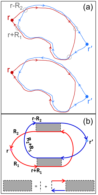
Figure 1: (a) Returning quasiparticle trajectories leading to the long-range correlations between the points $\mathbf{r}$ and $\mathbf{r}^{\prime}$. The trajectories are characterized by two pieces of long joint routes within which the diffusing particles move either in the same or in the opposite directions. (b)Two-diffuson diagram describing long-range part of the LDoS correlation function. Upper (lower) loop represents $G^{R}(E,\mathbf{r}^{\prime},\mathbf{r}^{\prime})$ ($G^{A}(E,\mathbf{r},\mathbf{r})$) correspondingly. Shaded box represents diffuson. The two-cooperon contribution can be obtained by reversing arrows direction in one of the loops.

The case of normal metal represents a natural starting point and a convenient reference. The effects of multiple scattering and quantum coherence on spatial correlations of LDoS in disordered normal metals were considered in Ref. Lerner, . It was found that two different contributions can be distinguished in the LDoS correlation function. The short-range contribution represents the Friedel oscillations modified by multiple impurity scattering. The second long-range contribution appears due coherent diffusive propagation of normal quasiparticles. In the following, we will focus namely on this long-range term and, for completeness, we start with reproduction of its calculation.

Our purpose is to evaluate the LDoS correlation function at the same energy

$$\mathcal{L}^{\left(\mathrm{n}\right)}(\mathbf{r}-\mathbf{r}^{\prime},E)=\left\langle N_{\mathrm{e}}^{\left(\mathrm{n}\right)}(E,\mathbf{r})N_{\mathrm{e}}^{\left(\mathrm{n}\right)}(E,\mathbf{r}^{\prime})\right\rangle-\left\langle N_{\mathrm{e}}^{\left(\mathrm{n}\right)}(E)\right\rangle^{2}.$$ (1)

As the LDoS per spin is related to the retarded Green’s function $G^{R}(E,\mathbf{r},\mathbf{r})$ by the standard relation,

$$N_{\mathrm{e}}^{\left(\mathrm{n}\right)}(E,\mathbf{r})=-\mathrm{Im}[G^{R}(E,\mathbf{r},\mathbf{r})]/\pi,$$ (2)

this quantity can be expressed via retarded and advanced Green’s functions:

$$\mathcal{L}^{\left(\mathrm{n}\right)}(\mathbf{r}-\mathbf{r}^{\prime},E)=\frac{1}{2\pi^{2}}\left\{\mathrm{Re}\left[\left\langle G^{R}(E,\mathbf{r},\mathbf{r})G^{A}(E,\mathbf{r}^{\prime},\mathbf{r}^{\prime})\right\rangle\right.\right.$$

$$\left.\left.-\left\langle G^{R}(E,0,0)\right\rangle\left\langle G^{A}(E,0,0)\right\rangle\right]\right.$$ (3)

$$\left.-\!\mathrm{Re}\left[\left\langle G^{R}(E,\mathbf{r},\mathbf{r})\ G^{R}(E,\mathbf{r}^{\prime},\mathbf{r}^{\prime})\right\rangle\!-\!\left\langle G^{R}(E,0,0)\right\rangle^{2}\right]\right\},$$

where $\langle\ldots\rangle$ implies averaging over impurities distribution. One can use this presentation for impurity averaging within the standard Green’s function approach. We will assume weak impurity scattering (Born limit). The contributions to the LDoS correlation function can be represented as diagrams consisting of two loops connected by impurity lines.

The long-range contribution to the LDoS correlation function is given by the sum of the two-diffuson and two-cooperon diagrams, $\mathcal{L}^{\left(\mathrm{n}\right)}=\mathcal{L}^{\left(\mathrm{n}\right)}_{(2D)}+\mathcal{L}^{\left(\mathrm{n}\right)}_{(2C)}$, see Fig. 1(b). Both of them give the same contributions, which can be approximately written as

$$\mathcal{L}^{\left(\mathrm{n}\right)}_{(2D)}(\mathbf{r}\!-\!\mathbf{r}^{\prime},E)=\mathcal{L}^{\left(\mathrm{n}\right)}_{(2C)}(\mathbf{r}\!-\!\mathbf{r}^{\prime},E)\approx\frac{\left|\mathcal{B}\left(E\right)\right|^{2}}{2\pi^{2}}C_{\mathrm{n}}^{2}(\mathbf{r}\!-\!\mathbf{r}^{\prime}),$$ (4)

where $C_{\mathrm{n}}(\mathbf{r}-\mathbf{r}^{\prime})$ is the cooperon,

$$\mathcal{B}^{\mathrm{(n)}}\left(E\right)=\int d\mathbf{R}_{1}\int d\mathbf{R}_{2}\bar{G}^{R}(\mathbf{R}_{1})\bar{G}^{A}(\mathbf{R}_{1}\mathbf{-\mathbf{R}}_{2})\bar{G}^{R}(\mathbf{R}_{2})$$ (5)

is the “Hikami box”, and

$$\bar{G}^{R,A}(\mathbf{R})\!\equiv\!\left\langle G^{R,A}(E,\mathbf{r},\mathbf{r}\!+\!\mathbf{R})\right\rangle\!=\!\int\frac{d^{D}\mathbf{p}}{(2\pi)^{D}}\frac{\exp(i\mathbf{pR})}{E\!-\!\epsilon_{\mathbf{p}}\pm i/2\tau}$$

are the averaged Green’s functions with $\mathrm{D}$ being the space dimensionality. Here $\tau$ is the elastic scattering time, $\epsilon_{\mathbf{p}}=v_{F}(p-p_{F})$, $v_{F}$ and $p_{F}$ are the Fermi velocity and momentum. Integration in Eq. (5) gives a very simple result

$$\mathcal{B}^{\mathrm{(n)}}\left(E\right)=2\pi i\nu\tau^{2}$$ (6)

with $\nu=\langle N_{\mathrm{e}}^{\left(\mathrm{n}\right)}(E,\mathbf{r})\rangle$ as the average value of LDoS.

Hence, the long-range behavior of the LDoS is completely determined by the cooperon $C_{\mathrm{n}}(\mathbf{r}-\mathbf{r}^{\prime})$ whose Fourier transform is well known WeakLocal

$$C_{\mathrm{n}}(q)=\frac{1}{2\pi\nu\tau}f_{\mathrm{D}}(lq)\ \text{with }f_{\mathrm{D}}(lq)\approx\frac{\mathrm{D}}{l^{2}q^{2}}\text{ for }lq\ll 1,$$ (7)

where $l=v_{F}\tau$ is the mean-free path. In real space

$$C_{\mathrm{n}}(r)=\frac{\mathrm{D}}{2\pi\nu\tau l^{\mathrm{D}}}\tilde{f}_{\mathrm{D}}(r/l).$$ (8)

At $r\gg l$

$$\tilde{f}_{\mathrm{D}}(r)\approx\frac{1}{\pi}\left\{\begin{array}[c]{cc}\ln(l_{\phi}/r)&\text{ for }\mathrm{D}=2\\ 3/4r&\text{for }\mathrm{D}=3\end{array}\right..$$ (9)

For the 2D case the logarithmic divergency is cut off at $q\sim 1/l_{\phi}$, where $l_{\phi}$ is the phase-decoherence length. As the Green’s functions decay at the distances of the order of the mean-free path, in order to evaluate the long-range behavior $|\mathbf{r}-\mathbf{r}^{\prime}|\gg l$, we replaced in Eq. (4) arguments of both cooperons with $|\mathbf{r}-\mathbf{r}^{\prime}|$.

Substituting the results (6) and (8) into Eq. (4), we obtain the long-range asymptotic expression of the LDoS correlation function Lerner

$$\mathcal{L}^{\left(\mathrm{n}\right)}(\mathbf{r}-\mathbf{r}^{\prime},E) =\left(2\nu\tau^{2}\right)^{2}C^{2}_{\mathrm{n}}(\mathbf{r}-\mathbf{r}^{\prime})$$

$$=\nu^{2}\frac{a_{\mathrm{D}}}{\left(k_{F}l\right)^{2\mathrm{D}-2}}f_{\mathrm{D}}^{2}(|\mathbf{r}-\mathbf{r}^{\prime}|/l)$$ (10)

with $a_{2}=4$ and $a_{3}=4\pi^{2}$. From this result we see that LDoS variations are small in comparison with the average DoS by the parameter $\left(k_{F}l\right)^{\mathrm{D}-1}$. It is important to stress that in contrast to the short-ranged Friedel oscillations, they decay slowly at large distances up to $l_{\phi}$, as $\ln^{2}(l_{\phi}/r)$ for the 2D case and as $1/r^{2}$ for the 3D case.

III s-wave superconductors

III.1 Potential impurities

We start consideration of superconducting state with the simplest situation of purely potential scattering and s-wave symmetry of the order parameter. In this case the inhomogeneous LDoS is directly related to its normal-state counterpart. Indeed, using eigenstates expansion, the normal-state LDoS can be represented as

$$N_{\mathrm{e}}^{\left(\mathrm{n}\right)}(E,\mathbf{r})=\sum_{i}|\psi_{i}(\mathbf{r})|^{2}\delta(E-E_{i}),$$ (11)

where $\psi_{i}(\mathbf{r})$ are eigenfunctions and $E_{i}$ are eigenenergies of the quasiparticle states. In case of potential scattering, the corresponding eigenenergies in superconducting state become $\pm\sqrt{E_{i}^{2}+\Delta^{2}}$ where $\Delta$ is the gap parameter, and the two-component Bogoliubov wave function of quasiparticle state in superconductor $(U_{i,\pm}(\mathbf{r}),V_{i,\pm}(\mathbf{r}))$ is proportional to the normal state wave function $(U_{i,\pm}(\mathbf{r}),V_{i,\pm}(\mathbf{r}))=(u_{i,\pm},v_{i\,,\pm})\psi_{i}(\mathbf{r}),$ where $u_{i,\pm}$ and $v_{i,\pm}$ are coordinate-independent constants $u_{i,\alpha}=\left(\alpha/\sqrt{2}\right)\sqrt{1+\alpha E_{i}/\sqrt{E_{i}^{2}+\Delta^{2}}}$, $v_{i,\alpha}=\left(1/\sqrt{2}\right)\sqrt{1-\alpha E_{i}/\sqrt{E_{i}^{2}+\Delta^{2}}}$, $|u_{i,\pm}|^{2}+|v_{i,\pm}|^{2}=1$.deGennes A quantity commonly evaluated for superconductors is the density of states for excitations which in normal state corresponds to symmetric combination $N_{\mathrm{ex}}^{\left(\mathrm{n}\right)}(E,\mathbf{r})=N_{\mathrm{e}}^{\left(\mathrm{n}\right)}(E,\mathbf{r})+N_{\mathrm{e}}^{\left(\mathrm{n}\right)}(-E,\mathbf{r})$. The excitation LDoS in superconducting state, $N_{\mathrm{ex}}^{\left(\mathrm{s}\right)}(E,\mathbf{r})$, can be represented in the form of eigenstate expansion as

$$N_{\mathrm{ex}}^{(\mathrm{s})}(E,\mathbf{r})\!=\!\!\!\!\sum_{i,\alpha=\pm 1}\!\!\!\left[|U_{i,\alpha}(\mathbf{r})|^{2}\!+\!|V_{i,\alpha}(\mathbf{r})|^{2}\right]\!\delta\!\left(\!E\!-\!\alpha\sqrt{E_{i}^{2}\!+\!\Delta^{2}}\right)$$

$$=\sum_{i,\alpha=\pm 1}|\psi_{i}(\mathbf{r})|^{2}\frac{|E|}{\sqrt{E^{2}\!-\!\Delta^{2}}}\delta\left(E_{i}\!-\!\alpha\sqrt{E^{2}-\Delta^{2}}\right)$$

$$=\frac{|E|}{\sqrt{E^{2}-\Delta^{2}}}N_{\mathrm{ex}}^{\left(\mathrm{n}\right)}(\sqrt{E^{2}-\Delta^{2}},\mathbf{r})$$ (12)

(in the second line we change the variable of the $\delta$-function). Such a simple connection between the normal and superconducting LDoS is one of consequences of the Anderson theorem and it provides the following relation between the normal-state and superconducting LDoS correlation functions

$$\mathcal{L}^{\mathrm{(s)}}_{\mathrm{ex}}(E,\mathbf{r})/{[\nu_{\mathrm{ex}}^{\mathrm{(s)}}(E)]^{2}}=\mathcal{L}^{\mathrm{(n)}}_{\mathrm{ex}}(\sqrt{E^{2}-\Delta^{2}},\mathbf{r})/(2\nu)^{2},$$ (13)

where $\nu_{\mathrm{ex}}^{\mathrm{(s)}}(E)=2\nu E/\sqrt{E^{2}-\Delta^{2}}$ is the average superconducting DoS for excitations and $\mathcal{L}^{\mathrm{(n)}}_{\mathrm{ex}}(E,\mathbf{r})\approx\mathcal{L}^{\mathrm{(n)}}(E,\mathbf{r})+\mathcal{L}^{\mathrm{(n)}}(-E,\mathbf{r})$. Even though in the following we only consider $\mathcal{L}^{\mathrm{(s)}}_{\mathrm{ex}}(E,\mathbf{r})$, for completeness we also present a useful general relation for the electronic LDoS,

$$N_{\mathrm{e}}^{\left(\mathrm{s}\right)}(E,\mathbf{r})=\sum_{i,\alpha=\pm 1}\!|U_{i\,,\alpha}(\mathbf{r})|^{2}\delta\left(E-\alpha\sqrt{E_{i}^{2}+\Delta^{2}}\right)$$

$$=\sum_{\alpha=\pm 1}\frac{E\!+\!\alpha\sqrt{E^{2}\!-\!\Delta^{2}}}{2\sqrt{E^{2}-\Delta^{2}}}N_{\mathrm{e}}^{\left(\mathrm{n}\right)}(\alpha\sqrt{E^{2}\!-\!\Delta^{2}},\mathbf{r})$$ (14)

In particular, this general relation allows immediately to reproduce the single-impurity result reported for the s-wave case in Ref. CapriottiPRB03, .

Even though the long-range tail of LDoS for disordered s-wave superconductors can be immediately obtained from the normal-state result, it is useful, nevertheless, to rederive it formally, within the Green’s function approach. This will allow us to generalize such an approach later for less trivial situations for which the above argument does not work any more.

The long-range contribution to the LDoS correlation function is again determined by the diagram shown in Fig. 1(b), but both the Green’s functions and cooperons now have the matrix structure. In order to calculate them, it is convenient to use Nambu formalism decomposing the Green’s functions over Pauli matrices $\hat{\tau}^{j}$ and the cooperons over the direct product $\hat{\tau}^{k}\otimes\hat{\tau}^{k^{\prime}}$ of them

$$G^{R,A} \rightarrow G_{\alpha\beta}^{R,A}=g_{j}^{R,A}\tau_{\alpha\beta}^{j}$$ (15a)

$$C^{\left(\mathrm{s}\right)} \rightarrow C^{\left(\mathrm{s}\right)}_{\alpha\beta,\gamma\delta}=C^{\left(\mathrm{s}\right)}_{kk^{\prime}}\tau_{\alpha\beta}^{k}\tau_{\gamma\delta}^{k^{\prime}}$$ (15b)

We assume summation with respect to repeated indices. Let us note that the Cooperon $4\times 4$ matrix $C^{\left(\mathrm{s}\right)}_{kk^{\prime}}$ in fact has the $2\times 2$ block structureKulik ; VarlamovDorinZhETF86 :

$$C^{\left(\mathrm{s}\right)}_{kk^{\prime}}=\left[\begin{array}[c]{cc}\widehat{C}^{\left(\mathrm{s}\right)}_{A}&0\\ 0&\widehat{C}^{\left(\mathrm{s}\right)}_{B}\end{array}\right].$$ (16)

For potential scattering the averaged superconducting Green’s functions are given by

$$\hat{G}^{R,A}\left(E,\mathbf{p}\right) =\frac{\alpha^{R,A}\left(E\hat{\tau}^{0}+\Delta\hat{\tau}^{1}\right)+\epsilon_{\mathbf{p}}\hat{\tau}^{3}}{(\alpha^{R,A})^{2}\left(E^{2}-\Delta^{2}\right)-\epsilon_{\mathbf{p}}^{2}},$$ (17)

$$\alpha^{R,A} =1\mp\frac{i}{2\tau\sqrt{E^{2}-\Delta^{2}}}.$$

and for real $\Delta$ they do not contain $\hat{\tau}^{2}$ component.

In this formalism it is convenient to deal with LDoS for excitations $N_{\mathrm{ex}}^{\left(\mathrm{s}\right)}$ which is related to the trace of the Green’s function

$$N_{\mathrm{ex}}^{\left(\mathrm{s}\right)}(E,\mathbf{r})=-\frac{1}{\pi}\mathrm{Im}\left[\mathrm{Tr}\ \hat{G}^{R}\left(E,\mathbf{r},\mathbf{r}\right)\right].$$ (18)

Comparing this equation with the previous normal state LDoS definition (2) one can see that $N_{\mathrm{ex}}^{\left(\mathrm{s}\right)}(E,\mathbf{r})$ has an additional factor two since it contains both electron and hole contributions. In particular, the average LDoS for excitations is given by $\nu_{\mathrm{ex}}^{\mathrm{(s)}}$. The corresponding expression for the two-cooperon diagram can be represented using the Pauli-matrices decomposition:

$$\mathcal{L}^{\mathrm{(s)}}_{\mathrm{ex}(2C)}=\frac{4}{2\pi^{2}}U_{km}U_{k^{\prime}m^{\prime}}^{\ast}C^{\left(\mathrm{s}\right)}_{kk^{\prime}}C^{\left(\mathrm{s}\right)}_{mm^{\prime}},$$ (19a)

$$U_{km}=\frac{1}{2}\mathrm{Tr}\left(\hat{\tau}^{i}\hat{\tau}^{k}\hat{\tau}^{n}\hat{\tau}^{m}\hat{\tau}^{j}\right)\mathcal{B}_{inj}^{\left(\mathrm{s}\right)},$$ (19b)

$$\mathcal{B}_{inj}^{\left(\mathrm{s}\right)}=\!\int\!d\mathbf{R}_{1}\!\int\!d\mathbf{R}_{2}g_{i}^{A}(\mathbf{R}_{1})g_{n}^{R}(\mathbf{R}_{1}\!-\!\mathbf{R}_{2})g_{j}^{A}(\mathbf{R}_{2}).$$ (19c)

The computational details of superconducting cooperon components are presented in Appendix A.1. It turns out that its singular components are related to the normal-state cooperon (7) as

$$C^{\left(\mathrm{s}\right)}_{ij}(\mathbf{q}) =\frac{E^{2}}{E^{2}\!-\!\Delta^{2}}\left(-\frac{\Delta}{E}\right)^{i+j}\frac{C_{\mathrm{n}}(\mathbf{q})}{2}\text{, for }i,j=0,1\text{ }$$ (20a)

$$C^{\left(\mathrm{s}\right)}_{33}(\mathbf{q}) =C_{\mathrm{n}}(\mathbf{q})/2$$ (20b)

One can see that in the limit of normal metal, $\Delta\rightarrow 0$, the only nonzero components remained are $C^{\left(\mathrm{s}\right)}_{00}$ and $C^{\left(\mathrm{s}\right)}_{33}$.

Computing the trace of five Pauli matrices in Eq. (19b), taking into account (i) symmetry of $\mathcal{B}_{inj}^{\left(\mathrm{s}\right)}$ with respect to indices $i$ and $j$ and (ii) the absence of $\hat{\tau}^{2}$ components in all decompositions (see Appendix C), we obtain

$$U_{km} =\delta_{m0}\mathcal{B}_{iki}^{\left(\mathrm{s}\right)}+\delta_{k0}\mathcal{B}_{imi}^{\left(\mathrm{s}\right)}+\left(\delta_{mk}-2\delta_{m0}\delta_{k0}\right)\mathcal{B}_{i0i}^{\left(\mathrm{s}\right)}$$

$$+2\left\{(1-\delta_{k0})\mathcal{B}_{0mk}^{\left(\mathrm{s}\right)}+(1-\delta_{m0})\mathcal{B}_{0km}^{\left(\mathrm{s}\right)}\right.$$

$$\left.-(1-\delta_{n0})\mathcal{B}_{0nn}^{\left(\mathrm{s}\right)}\left(\delta_{km}-2\delta_{k0}\delta_{m0}\right)\right\},$$

where summation with respect to the index $i=0,1,3$ is assumed in the first three terms. The components of the Hikami boxes are computed in Appendix A.2. For $i,j,m=0,1$

$$\mathcal{B}_{imj}^{\left(\mathrm{s}\right)}\!=\!-\frac{i\pi\nu\tau^{2}}{2}\frac{E^{3}\left(\sqrt{E^{2}\!-\!\Delta^{2}}+\frac{3i}{2\tau}\right)}{\left(E^{2}\!-\!\Delta^{2}\right)^{3/2}\!\left(\sqrt{E^{2}\!-\!\Delta^{2}}+\frac{i}{2\tau}\right)}\left(\frac{\Delta}{E}\right)^{i+j+m}\text{ }$$

and

$$\mathcal{B}_{033}^{\left(\mathrm{s}\right)} =-\frac{i\pi\nu E\tau^{2}}{2\sqrt{E^{2}-\Delta^{2}}},$$

$$\mathcal{B}_{303}^{\left(\mathrm{s}\right)} =-\frac{i\pi\nu E\tau^{2}}{2\sqrt{E^{2}-\Delta^{2}}}\frac{\sqrt{E^{2}-\Delta^{2}}-\frac{i}{2\tau}}{\sqrt{E^{2}-\Delta^{2}}\!+\!\frac{i}{2\tau}}.$$

Due to the specifics of the cooperon $C^{\left(\mathrm{s}\right)}_{ij}(\mathbf{q})$ structure for $i,j=0,1$, seen from Eq. (20a), we need only the combination $U_{00}+U_{11}\left(\Delta/E\right)^{2}-2\left(\Delta/E\right)U_{01}$ for which we find a very simple relation

$$U_{00}+U_{11}\left(\Delta/E\right)^{2}-2\left(\Delta/E\right)U_{01}=U_{33}\left[1-\left(\Delta/E\right)^{2}\right]$$

and for $U_{33}$ we derive

$$U_{33}=-2i\pi\nu\tau^{2}\frac{E}{\sqrt{E^{2}-\Delta^{2}}}.$$

Collecting terms, we finally obtain for the total correlation function, $\mathcal{L}^{\mathrm{(s)}}_{\mathrm{ex}}=\mathcal{L}^{\mathrm{(s)}}_{\mathrm{ex}(2C)}+\mathcal{L}^{\mathrm{(s)}}_{\mathrm{ex}(2D)}$,

$$\mathcal{L}^{\mathrm{(s)}}_{\mathrm{ex}}(\mathbf{r}-\mathbf{r}^{\prime},E)=\frac{4}{\pi^{2}}|U_{33}|^{2}$$

$$\times\left[\left(1-\left(\frac{\Delta}{E}\right)^{2}\right)^{2}[C^{\left(\mathrm{s}\right)}_{00}(\mathbf{r}-\mathbf{r}^{\prime})]^{2}+[C^{\left(\mathrm{s}\right)}_{33}(\mathbf{r}-\mathbf{r}^{\prime})]^{2}\right]$$

$$=2\left(\frac{2\nu\tau^{2}E}{\sqrt{E^{2}-\Delta^{2}}}\right)^{2}C^{2}_{\mathrm{n}}(\mathbf{r}-\mathbf{r}^{\prime}).$$ (21)

This result explicitly confirms the relation (13) based on Anderson-theorem arguments.

III.2 Magnetic impurities

In this section we evaluate the LDoS correlation function for s-wave superconductor with magnetic scatterers. Since the seminal paper of Abrikosov and Gor’kov AG60 it is established that the magnetic impurities dramatically suppress superconductivity and strongly influence the quasiparticle density of states. The original mean-field approach (AG theory) suggested that the hard gap in the average DoS is not eliminated by magnetic impurities. This hard gap decreases with increasing the magnetic-impurities concentration and vanishes at certain critical concentration so that the gapless superconducting state exists within small range of concentrations. More accurate later treatments beyond the mean-field approach Simons01 ; ShytovPRL03 have demonstrated that the low-energy quasiparticle states are in fact generated for all magnetic-impurities concentrations meaning that, strictly speaking, the hard gap is eliminated by any amount of magnetic impurities. For small concentrations, however, the average DoS at low energies have exponentially small tail.

Formally, in the presence of magnetic scattering the Green’s function can be still presented in the form similar to Eq. (17), but within the mean-field approach the renormalized energy and gap now are determined from the self-consistent transcendental equations.AG60 This result is usually obtained taking into account the spin structure of the superconductive Green’s function Maki , which means the additional increase of the matrix dimensionality to $4\times 4$. In the calculation of the two-cooperon diagrams in Nambu representation (19a) the number of Pauli matrices in traces is already large. That is why, for the sake of simplicity, we will consider below magnetic scatterers as Ising impurities oriented in the same direction. This allows us to preserve $2\times 2$ matrix structure of the Green’s function, which significantly simplifies calculations. The physical picture remains practically identical to the case of isotropic magnetic impurities. Even for such a minimum model describing the pair-breaking scattering, the calculations and results become rather cumbersome. Technically similar work has been done in Ref. SmithAmbegPRB00, where suppression of the transition temperature by magnetic impurities in combination with Coulomb effects has been investigated. This thermodynamic problem required summation of ladder diagrams with elastic and magnetic impurity lines in the Matsubara-frequency presentation. In principle, the cooperon components at real energies could be obtained from the results of this work via analytic continuation. However, this procedure is not trivial at all.

The long-range LDoS correlation function is still defined by Eq. (19a) but the Green’s functions, cooperons, and Hikami boxes are considerably modified by magnetic scattering. Detailed derivations of these objects are presented in Appendices B.1 and B.2. Instead of Eq. (17), Green’s functions are given by

$$\hat{G}^{R,A}\left(\mathbf{p}\right)=\frac{\tilde{E}_{\pm}\hat{\tau}^{0}+\tilde{\Delta}_{\pm}\hat{\tau}^{1}+\epsilon_{\mathbf{p}}\hat{\tau}^{3}}{\tilde{E}_{\pm}^{2}-\tilde{\Delta}_{\pm}^{2}-\epsilon_{\mathbf{p}}^{2}}$$ (22)

with the renormalized energy and gap

$$\tilde{E}_{\pm} =E\pm\frac{i\eta_{\pm}}{2\tau_{0}\sqrt{\eta_{\pm}^{2}-1}},$$ (23a)

$$\tilde{\Delta}_{\pm} =\Delta\pm\frac{i}{2\tau_{1}\sqrt{\eta_{\pm}^{2}-1}},$$ (23b)

where $$1/\tau_{\alpha}=1/\tau+(-1)^{\alpha}/\tau_{m} \tau \tau_{m} + - \eta_{\pm}=\tilde{E}_{\pm}/\tilde{\Delta}_{\pm}$$, and are the potential and magnetic scattering times. Here and below the subscript “” (“”) corresponds to the retarded (advanced) components. The parameter has to be determined from the equation

$$\eta_{\pm}\left(1\mp\frac{i}{\tau_{m}\Delta\sqrt{\eta_{\pm}^{2}-1}}\right)=\frac{E}{\Delta}.$$ (24)

The average DoS is connected with $\eta_{+}$ by relation AG60

$$\nu_{\mathrm{ex}}^{(\mathrm{sm})}(E)=2\nu\operatorname{Re}\frac{\eta_{+}}{\sqrt{\eta_{+}^{2}-1}}.$$ (25)

The $2\times 2$ blocks of the cooperon Eq. (16) computed in Appendix B.1 are

$$\hat{C}_{A}^{\mathrm{(sm)}}= \frac{1/4\pi\nu}{1-\tilde{\gamma}_{\mathbf{q}}}\left[\left(\frac{1}{\tau_{m}}\!+\!\frac{\chi_{1}\tilde{\gamma}_{\mathbf{q}}}{2\tau^{\ast}}\right)\hat{\tau}^{0}\right.$$

$$\left.+\left(\frac{1}{\tau}\!-\!\frac{\tilde{\gamma}_{\mathbf{q}}}{2\tau^{\ast}}\right)\hat{\tau}^{3}\!-\!\frac{\tilde{\gamma}_{\mathbf{q}}}{\tau^{\ast}}\frac{\operatorname{Re}\eta_{+}}{\left|\eta_{+}^{2}-1\right|}\hat{\tau}^{1}\right]$$ (26)

and

$$\hat{C}_{B}^{\mathrm{(sm)}}= \frac{1/4\pi\nu}{1-\tau_{\mathrm{qp}}\tilde{\gamma}_{\mathbf{q}}\left(\frac{1}{\tau}+\frac{\chi_{2}}{\tau_{m}}\right)}\left[\left(\frac{1}{\tau_{m}}+\frac{\chi_{2}\tilde{\gamma}_{\mathbf{q}}}{2\tau^{\ast}}\right)\hat{\tau}^{0}\right.$$

$$- \left.\left(\frac{1}{\tau}-\frac{\tilde{\gamma}_{\mathbf{q}}}{2\tau^{\ast}}\right)\hat{\tau}^{3}+i\frac{\tilde{\gamma}_{\mathbf{q}}}{\tau^{\ast}}\frac{\operatorname{Im}\eta_{+}}{\left|\eta_{+}^{2}-1\right|}\hat{\tau}^{2}\right]$$ (27)

with

$$\tau_{\mathrm{qp}}^{-1} =\frac{1}{\tau}+\frac{\chi_{1}}{\tau_{m}},\ \chi_{1}=\frac{|\eta_{+}|^{2}+1}{\left|\eta_{+}^{2}-1\right|},\ \chi_{2}=\frac{|\eta_{+}|^{2}-1}{\left|\eta_{+}^{2}-1\right|},\$$

$$\tilde{\gamma}_{\mathbf{q}} =\left\langle\frac{1}{1+\tau_{\mathrm{qp}}^{2}\left(\mathbf{v}_{F}\mathbf{q}\right)^{2}}\right\rangle,\;\frac{1}{\tau^{\ast}}=\tau_{\mathrm{qp}}\left(\frac{1}{\tau^{2}}-\frac{1}{\tau_{m}^{2}}\right).$$

Note that the component $\hat{C}_{A}^{\mathrm{(sm)}}$ still has diffusive divergency for $q\rightarrow 0$, while in $\hat{C}_{B}^{\mathrm{(sm)}}$ it is cut off by magnetic scattering. Finally, we compute the Hikami-box components

$$\mathcal{B}_{000}^{\left(\mathrm{sm}\right)} =-\frac{i\pi\nu\tau_{\mathrm{qp}}^{2}}{2}\frac{\tilde{E}_{+}^{2}\tilde{E}_{-}\left(\sqrt{\tilde{E}_{+}^{2}-\tilde{\Delta}_{+}^{2}}+\frac{i}{\tau_{\mathrm{qp}}}\right)}{\left[\tilde{E}_{+}^{2}-\tilde{\Delta}_{+}^{2}\right]^{3/2}\sqrt{\tilde{E}_{-}^{2}-\tilde{\Delta}_{-}^{2}}},$$

$$\mathcal{B}_{klm}^{\left(\mathrm{sm}\right)} =\mathcal{B}_{000}^{\left(\mathrm{sm}\right)}\zeta_{+}^{k+m}\zeta_{-}^{l},\ \text{for\ }k,l,m=0,1$$

with notations $\zeta_{+}=\tilde{\Delta}_{+}/\tilde{E}_{+}=1/\eta_{+}$ and

$$\mathcal{B}_{k33}^{\left(\mathrm{sm}\right)} =-\frac{i\pi\nu\tau_{\mathrm{qp}}^{2}}{2}\frac{\tilde{E}_{+}\zeta_{+}^{k}}{\sqrt{\tilde{E}_{+}^{2}-\tilde{\Delta}_{+}^{2}}}=-\frac{i\pi\nu\tau_{\mathrm{qp}}^{2}}{2}\frac{\eta_{+}\zeta_{+}^{k}}{\sqrt{\eta_{+}^{2}-1}}$$

$$\mathcal{B}_{3k3}^{\left(\mathrm{sm}\right)} =-\frac{i\pi\nu\tau_{\mathrm{qp}}^{2}}{2}\frac{\tilde{E}_{-}\zeta_{-}^{k}}{\sqrt{\tilde{E}_{+}^{2}-\tilde{\Delta}_{+}^{2}}}$$

for $k=0,1$.

Taking into account all these modifications, one can calculate the LDoS correlation function in the presence of magnetic impurities. Its long-ranged part comes from the A-block only (as it was already mentioned, the divergence at $q\rightarrow 0$ in $\widehat{C}_{B}$ is cut off by paramagnetic impurities, see Eq.(51) ) and the final answer can be represented as

$$\mathcal{L}^{\mathrm{(sm)}}_{\mathrm{ex}}(\mathbf{r}-\mathbf{r}^{\prime},E)=\left(2\nu\tau_{0}^{2}\right)^{2}\left|\mathcal{R}\right|^{2}C^{2}_{\mathrm{n}}(\mathbf{r}-\mathbf{r}^{\prime}),$$ (28)

where $1/\tau_{0}=1/\tau+1/\tau_{m}$, $C_{\mathrm{n}}(\mathbf{r}-\mathbf{r}^{\prime})$ is the normal-state cooperon (7) and

$$\mathcal{R}=\frac{\chi_{1}+1}{4}\frac{1+\tau/\tau_{m}}{1+\chi_{1}\tau/\tau_{m}}$$ (29)

$$\times\left\{\frac{1+\vartheta^{2}-2\vartheta\zeta_{-}}{\sqrt{1-\zeta_{-}^{2}}}+\frac{1-\vartheta^{2}}{\sqrt{1-\zeta_{+}^{2}}}+\frac{2\zeta_{+}}{1-\zeta_{+}^{2}}\left(\frac{2}{\sqrt{1-\zeta_{-}^{2}}}-\frac{\tilde{E}_{-}}{\tilde{E}_{+}}\frac{1}{\sqrt{1-\zeta_{+}^{2}}}\right)\left[\left(1+\vartheta^{2}\right)\operatorname{Re}[\zeta_{+}]-\vartheta\left(1+\zeta_{+}\zeta_{-}\right)\right]\right\}$$

with

$$\vartheta=r\sqrt{\frac{\chi_{1}-1}{\chi_{1}+1}},\ \frac{\tilde{E}_{-}}{\tilde{E}_{+}}=\frac{-\frac{E}{\Delta}r+\eta_{-}}{-\frac{E}{\Delta}r+\eta_{+}},\ r=\frac{1-\tau/\tau_{m}}{1+\tau/\tau_{m}}.$$

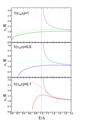
Figure 2: Examples of the energy dependences of the normalized average DoS $\nu_{\mathrm{ex}}^{(\mathrm{sm})}(E)/(2\nu)$, Eq. (25), (solid lines), and function $|\mathcal{R}(E)|$, Eq. (29), (dashed lines), which determines the long-range LDoS correlations for $1/(\tau\Delta)=5$ and different values of $1/(\tau_{m}\Delta)$. Dash-dotted lines show for reference the BCS density of states.

Normalization of the dimensionless function $\mathcal{R}(E)$ is selected by the condition $\mathcal{R}(E)\rightarrow 1$ for $E\rightarrow\infty$. This function together with normalized average DoS is plotted in Fig. 2 for several values of the pair-breaking parameter $1/(\tau_{m}\Delta)$. As one can see, the energy dependence of the correlation function described by $\mathcal{R}(E)$ is quite different from that one of average density of states. The most dramatic disparity is observed at small concentration of magnetic impurities, for $1/(\tau_{m}\Delta)=0.1$. In this case the function $\mathcal{R}(E)$ monotonically increases with decrease of energy, while $\nu(E)$ goes down and finally vanishes at $E\approx 0.7\Delta$. Here, at the edge of local density of states gap, the function $\mathcal{R}(E)$ reaches its maximum. With increase of magnetic impurities concentration, when $1/(\tau_{m}\Delta)=0.5$, the function $\mathcal{R}(E)$ still passes noticeably above $\nu(E)$, reaches its weakly pronounced maximum and remains finite when $\nu(E)$ turns zero. The behavior of both functions becomes almost similar only in the gapless state, when $1/(\tau_{m}\Delta)=1$. From these plots we can conclude that, in contrast to elastic impurities, the ratio $\mathcal{L}^{\mathrm{(sm)}}(E)/(\nu(E))^{2}$ increases with decreasing energy, i.e., relative LDoS variations become stronger at smaller energy. We also found that at the point where the mean-field average DoS vanishes, the correlation function remains finite. Note again that the vanishing of the average DoS is not exact result but only a consequence of the mean-field approximation. In reality, the mean-field gap point marks the approximate location of transition between delocalized quasiparticles and the Lifshitz-tail region corresponding to localized quasiparticles.Simons01 ; ShytovPRL03 Calculation of the LDoS correlation function is beyond the mean-field approach. As $\mathcal{L}(E)$ increases with decreasing the diffusion constant, the found growth of $\mathcal{L}^{\mathrm{(sm)}}(E)$ with decreasing energy can be interpreted as indication of slowing down diffusion when energy approaches the mobility edge. On the other hand, our calculation is only applicable to delocalized diffusive quasiparticles. One can expect that in the tail region the LDoS correlation function should decay exponentially at the localization length. Therefore measurements of the LDoS correlation function can be used to locate the mobility edge separating delocalized and localized states.

IV d-wave superconductors

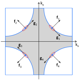
Figure 3: Schematic Fermi surface for a cuprate d-wave superconductor. $\mathbf{f}_{n}$ and $\mathbf{g}_{n}$ represent, respectively, the unity vectors parallel to the Fermi velocity $\mathbf{v}_{\mathrm{f}}$ and the “gap velocity” $\mathbf{v}_{\mathrm{g}}$ at the n-th gap node. The ellipses illustrate the constant-energy surfaces near the nodes.

Finally, let us consider the inhomogeneous LDoS for superconductors with d-wave symmetry of the order parameter, which is of special interest because of its relevance to cuprate high-temperature superconductors. Behavior of LDOS in these materials was extensively studied by STM.STMcupr Formally, the long-range LDoS correlation function is still determined by the general Eq. (19a) but the specifics of nodal gap structure has to be taken into account.

We consider a two-dimensional d-wave superconductor with electronic spectrum $\epsilon(k_{x},k_{y})$ defined within the square Brillouin zone $|k_{x}|,|k_{y}|<\pi/a$ and characterized by the bandwidth $t\!=\!\epsilon(\pi/a,0)-\epsilon(0,0)$, where $a$ is the lattice constant. Figure 3 illustrates the typical Fermi surface of a cuprate superconductor dwaveFS which, as usual, is determined by the equation $\epsilon(k_{x},k_{y})=\mu$, where $\mu$ is the chemical potential. The order parameter of the d${}_{\mathrm{x^{2}-y^{2}}}$-wave pairing state is expressed by

$$\Delta_{\mathbf{k}}=\Delta_{0}\left[\cos(k_{x}a)-\cos(k_{y}a)\right].$$

The gap nodes correspond to the points $\mathbf{k}_{n}=\pm\left(k_{0}\pm k_{0}\right)$ ($n=1,2,3,4$), where $k_{0}$ is determined by $\epsilon(k_{0},k_{0})=\mu$. The quasiparticle spectrum is given by $\varepsilon_{\mathbf{k}}\!=\sqrt{\xi_{\mathbf{k}}^{2}+\Delta_{\mathbf{k}}^{2}}$ with $\xi_{\mathbf{k}}\!=\epsilon(k_{x},k_{y})\!-\!\mu$ and close to the gap nodes it can be linearized as $\varepsilon_{\mathbf{k}}\approx\sqrt{(v_{\mathrm{f}}\tilde{k}_{\mathrm{f}})^{2}+(v_{\mathrm{g}}\tilde{k}_{\mathrm{g}})^{2}}$, where $\tilde{\mathbf{k}}$ is the momentum measured from the node $\mathbf{k}_{n}$ and $v_{\mathrm{g}}\!\approx v_{\mathrm{f}}\Delta_{0}/t\!\ll\!v_{\mathrm{f}}$. The directions of the Fermi velocity $\mathbf{v}_{\mathrm{f}}$ and “gap velocity” $\mathbf{v}_{\mathrm{g}}$ are depicted in Fig. 3.

The weak-localization effects for d-wave superconductors were considered in Refs. YashenkinPRL01, and YangPRB04, for arbitrarily strong impurity scattering. Here we limit ourselves with the simplest situation of weak isotropic scattering by non-magnetic elastic impurities. The one-particle Green’s function has the same matrix structure as general Eq. (17):

$$G_{\mathbf{k}}^{R,A}\left(E\right)=\frac{\left[\tilde{\epsilon}\pm i\gamma\right]\tau_{0}+\Delta_{\mathbf{k}}\tau_{1}+\xi_{\mathbf{k}}\tau_{3}}{\left[\tilde{\epsilon}\pm i\gamma\right]^{2}-\varepsilon_{\mathbf{k}}^{2}}.$$ (30)

Here $\tilde{\epsilon}$ is the effective energy renormalized by scattering, $\gamma=\gamma\left(\tilde{\epsilon}\right)$ is the impurity-induced relaxation rate. Both of them are self-consistently determined by the self-energy part $\tilde{\epsilon}\pm i\gamma\left(\tilde{\epsilon}\right)=E-\Sigma_{0}^{\pm}\left(\tilde{\epsilon}\right)$, with

$$\Sigma_{0}^{\pm}\left(\tilde{\epsilon}\right)=uN_{n}\int\int\frac{dk_{x}}{2\pi}\frac{dk_{y}}{2\pi}\frac{\tilde{\epsilon}\pm i\gamma\left(\tilde{\epsilon}\right)}{\left(\tilde{\epsilon}\pm i\gamma\left(\tilde{\epsilon}\right)\right)^{2}-\varepsilon_{\mathbf{k}}^{2}},$$ (31)

$N_{n}$ being the number of nodes (=4 in our case), and integration is limited by the region near one node. Performing integration in Eq. (31) with the above quasiparticle spectrum $\varepsilon_{\mathbf{k}}$ and separating the imaginary part of $\Sigma_{0}^{\pm}\left(\tilde{\epsilon}\right)$ one finds the transcendental equation for determination of the relaxation rate $\gamma(\tilde{\epsilon})$:

$$\ln\frac{\Delta_{0}}{\sqrt{\tilde{\epsilon}^{2}+\gamma^{2}}}+\frac{\tilde{\epsilon}}{\gamma}\arctan\frac{\tilde{\epsilon}}{\gamma}=\frac{2\pi v_{\mathrm{f}}v_{\mathrm{g}}}{uN_{n}}.$$ (32)

At zero energy it reproduces the known resultGorkovKalugZhETF85 ; PLeePRL93 ; DahmPRB05 ,

$$\gamma(0)=\gamma_{0}=\Delta_{0}\exp\left(-\frac{2\pi v_{\mathrm{f}}v_{\mathrm{g}}}{uN_{n}}\right),$$

while at large energies

$$\gamma\left(\tilde{\epsilon}\gg\gamma_{0}\right)\approx\frac{\pi}{2}\frac{\tilde{\epsilon}}{\ln(\tilde{\epsilon}/\gamma_{0})+1}\text{ }.$$

The real part of $\Sigma_{0}^{+}$ determines the value of $\tilde{\epsilon}$:

$$\tilde{\epsilon}-\frac{uN_{n}}{2\pi v_{\mathrm{f}}v_{\mathrm{g}}}\left(\tilde{\epsilon}\ln\frac{\Delta_{0}}{\sqrt{\gamma^{2}+\tilde{\epsilon}^{2}}}-\gamma\arctan\frac{\tilde{\epsilon}}{\gamma}\right)=E.$$ (33)

For small $E$, $\tilde{\epsilon}=\ln(\Delta_{0}/\gamma_{0})E$. When the energy is large ($E\gg\gamma_{0})$

$$\tilde{\epsilon}\approx E\frac{\ln\left(\Delta_{0}/\gamma_{0}\right)}{\ln\left(\tilde{\epsilon}/\gamma_{0}\right)}.$$

As follows from the structure of Eqs. (32) and (33), the energy dependences of $\tilde{\epsilon}$ and $\gamma$ have scaling form, $\tilde{\epsilon}=\gamma_{0}\mathcal{G}_{\epsilon}[\ln(\Delta_{0}/\gamma_{0})E/\gamma_{0}]$, $\gamma=\gamma_{0}\mathcal{G}_{\gamma}[\ln(\Delta_{0}/\gamma_{0})E/\gamma_{0}]$. These dependences are presented in Fig. 4(a)

The LDoS in superconducting state is determined by the integral of the imaginary part of the Green’s function (30) which givesDurstLeePRB00

$$N_{\mathrm{ex}}^{\left(\mathrm{d}\right)}(E)=\frac{N_{n}}{2\pi^{2}v_{\mathrm{f}}v_{\mathrm{g}}}\left(\gamma\ln\frac{\Delta_{0}^{2}}{\tilde{\epsilon}^{2}+\gamma^{2}}+2\tilde{\epsilon}\arctan\frac{\tilde{\epsilon}}{\gamma}\right).$$ (34)

The structure of cooperon for d-wave superconductors has been investigated in Ref. YashenkinPRL01, ; YangPRB04, . It was demonstrated that only diagonal components of the cooperon $C^{\mathrm{(sd)}}_{kk}$ in the Pauli-matrix expansion, Eq. (15b), are singular and these singular components are connected by relation $C^{\mathrm{(sd)}}_{00}=C^{\mathrm{(sd)}}_{11}=-C^{\mathrm{(sd)}}_{22}=C^{\mathrm{(sd)}}_{33}$. Therefore the matrix structure of d-wave cooperon is different from structure of the s-wave cooperon, Eq. (20). Derivation of the singular cooperon $C_{\mathrm{d}}(q)\equiv C^{\mathrm{(sd)}}_{00}(q)$ for arbitrary energy is presented in Appendix D.1 and result can be presented as

$$C_{\mathrm{d}}(q)=\frac{\gamma^{2}}{\pi N_{\mathrm{ex}}^{\left(\mathrm{d}\right)}\mathcal{D}q^{2}}$$ (35)

where parameters $\gamma$, $N_{\mathrm{ex}}^{\left(\mathrm{d}\right)}$, and the diffusion coefficient $\mathcal{D}$ are energy dependent with

$$\mathcal{D}\left(E\right)=\frac{\langle v^{2}\rangle}{2\gamma}\frac{1+\frac{\tilde{\epsilon}}{\gamma}\arctan\frac{\tilde{\epsilon}}{\gamma}}{\ln\frac{\Delta_{0}}{\sqrt{\tilde{\epsilon}^{2}+\gamma^{2}}}+\frac{\tilde{\epsilon}}{\gamma}\arctan\frac{\tilde{\epsilon}}{\gamma}}.$$ (36)

Note that our result for $C_{\mathrm{d}}(q)$ is smaller by factor four than the result of Refs. YashenkinPRL01, ; YangPRB04, . The origin of this discrepancy is discussed in Appendix D.1. For more transparent representation of the energy dependence in Eq. (35), we note a useful relation

$$N_{\mathrm{ex}}^{\left(\mathrm{d}\right)}(E)\mathcal{D}(E)=N_{\mathrm{ex}}^{\left(\mathrm{d}\right)}(0)\mathcal{D}(0)[1+(\tilde{\epsilon}/\gamma)\arctan(\tilde{\epsilon}/\gamma)].$$

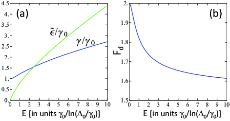
Figure 4: (a)The energy dependences of the parameter $\tilde{\epsilon}$ and the relaxation rate $\gamma$. (b) The energy dependence of the function $F_{d}$ which determines the LDoS correlation function in Eq. (38)

.

Calculation of the Hikami boxes $\mathcal{B}_{inj}^{\left(\mathrm{d}\right)}$ defined by Eq. (19c) with Green’s functions (30) (see Appendix D.2), results in:

$$\mathcal{B}_{000}^{\left(\mathrm{d}\right)} =\frac{N_{n}}{v_{\mathrm{f}}v_{\mathrm{g}}}\left[\tilde{\epsilon}+i\gamma\right]^{2}\left[\tilde{\epsilon}-i\gamma\right]J^{(0)},$$

$$\mathcal{B}_{101}^{\left(\mathrm{d}\right)} =\mathcal{B}_{303}^{\left(\mathrm{d}\right)}=\frac{N_{n}}{v_{\mathrm{f}}v_{\mathrm{g}}}\left[\tilde{\epsilon}-i\gamma\right]J^{(2)},$$

$$\mathcal{B}_{330}^{\left(\mathrm{d}\right)} =\mathcal{B}_{033}^{\left(\mathrm{d}\right)}=\mathcal{B}_{011}^{\left(\mathrm{d}\right)}=\mathcal{B}_{110}^{\left(\mathrm{d}\right)}=\frac{N_{n}}{v_{\mathrm{f}}v_{\mathrm{g}}}\left[\tilde{\epsilon}+i\gamma\right]J^{(2)},$$

where

$$J^{(0)} =-\frac{i}{16\pi\left(\tilde{\epsilon}+i\gamma\right)^{2}\tilde{\epsilon}\gamma}\left[1+\frac{\left(\tilde{\epsilon}+i\gamma\right)^{2}}{\tilde{\epsilon}\gamma}\arctan\frac{\tilde{\epsilon}}{\gamma}\right],$$

$$J^{(2)} =-\frac{i}{32\pi\tilde{\epsilon}\gamma}\left[1+\frac{\left(\tilde{\epsilon}-i\gamma\right)^{2}}{\tilde{\epsilon}\gamma}\arctan\frac{\tilde{\epsilon}}{\gamma}\right].$$

Further summation of these, non-zero, components of $\mathcal{B}_{inj}^{\left(\mathrm{d}\right)}$ in Eq. (19b) with corresponding traces of five Pauli-matrices products as the coefficients allows to present the tensor $U_{km}$ in the diagonal form $U_{km}^{\left(\mathrm{d}\right)}=U_{k}\delta_{km}$ with

$$U_{0;2} =\mathcal{B}_{000}^{\left(\mathrm{d}\right)}+2\mathcal{B}_{101}^{\left(\mathrm{d}\right)}\pm 4\mathcal{B}_{011}^{\left(\mathrm{d}\right)}$$

$$U_{1;3} =\mathcal{B}_{000}^{\left(\mathrm{d}\right)}+2\mathcal{B}_{101}^{\left(\mathrm{d}\right)}.$$

In result, the LDoS correlation function Eq. (19a) for the d-wave case takes the form

$$\mathcal{L}_{\mathrm{ex}}^{\mathrm{(d)}}(\mathbf{r}\!-\!\mathbf{r}^{\prime},E)\!=\!\frac{8}{\pi^{2}}\left[\left|\mathcal{B}_{000}^{\left(\mathrm{d}\right)}\!+\!2\mathcal{B}_{101}^{\left(\mathrm{d}\right)}\right|^{2}\!+\!8|\mathcal{B}_{011}^{\left(\mathrm{d}\right)}|^{2}\right]C_{\mathrm{d}}^{2}(\mathbf{r}\!-\!\mathbf{r}^{\prime})$$

$$=\frac{[N_{n}^{2}\gamma\left(\tilde{\epsilon}\right)]^{2}}{8\pi^{4}v_{\mathrm{f}}^{2}v_{\mathrm{g}}^{2}\gamma_{0}^{4}}F_{\mathrm{d}}\left(\frac{\tilde{\epsilon}}{\gamma\left(\tilde{\epsilon}\right)}\right)C_{\mathrm{d}}^{2}(\mathbf{r}\!-\!\mathbf{r}^{\prime},E=0),$$ (37)

with $\gamma\left(\tilde{\epsilon}\right)$ and $\tilde{\epsilon}(E)$ have to be determined from Eqs. (32) and (33),

$$F_{\mathrm{d}}(x) =\frac{1+1/x^{2}}{\left(1+x\arctan x\right)^{2}}\left\{\frac{3}{2}\left[1+\frac{x^{2}-1}{x}\arctan x\right]^{2}\right.$$

$$\left.+2\arctan^{2}x\right\}=\left\{\begin{tabular}[c]{ll}$2$&for $x=0$\\ $3/2$&for $x\gg 1$\end{tabular}\ \ \right.,$$

and the zero-energy cooperon in real space is given by

$$C_{\mathrm{d}}(r,E=0)=\frac{4\pi}{N_{n}}\frac{v_{\mathrm{f}}v_{\mathrm{g}}\gamma_{0}^{2}}{\left\langle v^{2}\right\rangle}\ln\frac{l_{\phi}}{r}.$$

Using this result, we can rewrite LDoS correlation function in a more transparent form

$$\mathcal{L}^{\mathrm{(d)}}_{\mathrm{ex}}(\mathbf{r}\!-\!\mathbf{r}^{\prime},E)=[N_{\mathrm{ex}}^{\left(\mathrm{d}\right)}(E)]^{2}F_{\mathrm{d}}\left(\frac{\tilde{\epsilon}}{\gamma}\right)$$

$$\times\frac{u^{2}}{32\pi^{2}\left\langle v^{2}\right\rangle^{2}}\ln^{2}\frac{l_{\phi}}{|\mathbf{r}-\mathbf{r}^{\prime}|}$$ (38)

We can see that, in contrast to s-wave superconductors with potential impurities, the energy dependence of the correlation function is not determined by the average density of states. Additional dependence characterized by the function $F_{\mathrm{d}}[\tilde{\epsilon(E)}/\gamma(E)]$ appears. Both the ratio $\tilde{\epsilon}/\gamma$ and function $F_{d}$ have universal dependences on the scaled energy $(E/\gamma_{0})\ln(\Delta_{0}/\gamma_{0})$. The energy dependence of $F_{d}$ is plotted in Fig. 4(b). We observe the same tendency as for an s-wave superconductor with magnetic impurities: the relative LDoS variations become stronger at smaller energies.

V Discussion

It is known that observable quantities of disordered metallic systems exhibit large mesoscopic fluctuations.Mesosc The large-scale correlations of the LDoS demonstrates long tails extending up to $r\sim l_{\phi}$.AKL As we have seen above, due to diffusive propagation of quasiparticles, such property of the LDoS correlation function remains valid also in superconductive state. This correlation function for all cases depends on scatterers potential $V$ in the same way: $\mathcal{L}\sim V^{4}$ and its spatial dependence is determined only by the dimensionality of superconductor. Our analysis demonstrates, however, that the energy dependence of the large-scale LDoS correlations carries valuable information about the order parameter symmetry and character of scattering in various superconductive systems. Indeed, as we have seen above, while the spatial dependence of $\mathcal{L}(\mathbf{r}\!-\!\mathbf{r}^{\prime},E)$ is the same for all types of considered superconducting systems and is determined by the square of normal-metal cooperon, the energy dependence of the magnitude of such correlator can serve as the fingerprint of superconductor intrinsic properties. In the reference case of s-wave superconductor with elastic impurities such energy dependence is just given by the square of the BCS quasi-particle density of states. More complex symmetry of the order parameter manifests itself in significant changes of the energy dependence of LDoS correlation function. Investigated above the case of d-wave pairing (see Fig. 4(b)), demonstrated that the corresponding LDoS correlation function, normalized on the appropriate square of the LDoS, already depends on the quasi-particle energy, although this dependence is rather smooth.

To illustrate the role of pair-breaking scattering, we analyzed the case of s-wave superconductor containing magnetic impurities. It is worth to discuss our results in light of the extended AG theory in Ref. Simons01, , which investigated the low-energy behavior of the average DoS in the framework of the nonlinear sigma model. The authors of Ref. Simons01, demonstrate, that AG results, establishing the formation of the hard gap in the local density of states, correspond to the saddle-point solution of the proposed effective action. Their non-perturbative extension beyond the mean-field approximation results in appearance of sub-gap exponential tails in the density of states, what should lead also to appearance of nonzero moments of this physical value for energies below the AG gap. Plausibly, our perturbative calculus of the second moment of local densities of states $\mathcal{L}^{(\mathrm{sm})}(\mathbf{r}-\mathbf{r}^{\prime},E)$ (see Fig. 2) indicates the same phenomenon. Our analysis allows for a straightforward generalization to other similar situations, such as interband scattering in multiband superconductors with different signs of order parameter in different bands ($s_{\pm}$ state), a widely discussed model for iron pnictides and selenides.

Modern STM technique, in principle, allows to probe the long-range correlations studied theoretically in this article. The challenge is to perform scan over large areas with sizes exceeding mean-free path. Another interesting opportunity provided by STM measurements of the LDoS correlation function is to extract and study the temperature-depending phase-breaking length $l_{\phi}(T)$ of quasiparticle excitations in superconductors of different nature. As far as we know, such a problem was never considered neither theoretically nor experimentally.

Appendix A s-wave superconductor with elastic impurities

A.1 Calculation of s-wave cooperon

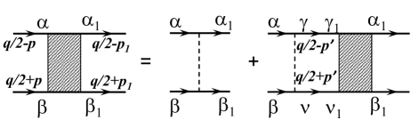
Figure 5: Graphic presentation of Eq. (39) for the superconducting cooperon.

In this Appendix we consider the cooperon structure for a s-wave superconductor with weak potential scattering. The superconducting cooperon has four Nambu indices and obeys the equation graphically represented Fig. 5,

$$C_{\beta\beta_{1}}^{\alpha\alpha_{1}} =u_{\beta\beta_{1}}^{\alpha\alpha_{1}}+u_{\beta\nu}^{\alpha\gamma}\Pi_{\nu\nu_{1}}^{\gamma\gamma_{1}}C_{\nu_{1}\beta_{1}}^{\gamma_{1}\alpha_{1}}$$ (39)

$$\Pi_{\nu\nu_{1}}^{\gamma\gamma_{1}} =\int\frac{d^{D}\mathbf{p}}{(2\pi)^{D}}\hat{G}_{\gamma\gamma_{1}}^{A}(\mathbf{p})\hat{G}_{\nu\nu_{1}}^{R}(\mathbf{p}-\mathbf{q})$$

where we again assume summation with respect to repeated Nambu indices. Here the superconducting Green’s functions $\hat{G}^{R,A}$ averaged over impurities are given by Eq. (17). For Born potential impurities, the matrix impurity line is given by

$$u_{\beta\beta_{1}}^{\alpha\alpha_{1}}=u\hat{\tau}_{\alpha\alpha_{1}}^{3}\hat{\tau}_{\beta\beta_{1}}^{3}\text{, }$$

with $u=n_{i}V^{2}=1/(2\pi\nu\tau)$.

To proceed, we represent the matrix impurity line as

$$u_{\beta\beta_{1}}^{\alpha\alpha_{1}} =\sum_{i,j=0}^{3}u_{ij}\hat{\tau}_{\alpha\beta}^{i}\hat{\tau}_{\beta_{1}\alpha_{1}}^{j}$$ (40)

$$\text{with }u_{ij} =\frac{u}{2}E_{ji}^{(33)},$$

where, following Refs. Kulik, ; VarlamovDorinZhETF86, , we introduced notation for the trace of four Pauli matrices

$$E_{lm}^{(ij)}\equiv\frac{1}{2}\mathrm{Tr}\left(\hat{\tau}^{i}\hat{\tau}^{l}\hat{\tau}^{j}\hat{\tau}^{m}\right)\text{.}$$

We will need only the following components of $E_{ml}^{(ij)}$ which have a simple block structure Kulik ; VarlamovDorinZhETF86

$$\hat{E}^{(00)} =\begin{bmatrix}\hat{\tau}^{0}&0\\ 0&\hat{\tau}^{0}\end{bmatrix},\ \hat{E}^{(11)}=\begin{bmatrix}\hat{\tau}^{0}&0\\ 0&-\hat{\tau}^{0}\end{bmatrix},\ \hat{E}^{(33)}=\begin{bmatrix}\hat{\tau}^{3}&0\\ 0&-\hat{\tau}^{3}\end{bmatrix}$$

$$\hat{E}^{(01)} =\begin{bmatrix}\hat{\tau}^{1}&0\\ 0&\hat{\tau}^{2}\end{bmatrix},\ \hat{E}^{(10)}=\begin{bmatrix}\hat{\tau}^{1}&0\\ 0&-\hat{\tau}^{2}\end{bmatrix}$$

Since $E_{ij}^{(33)}$ is diagonal, we have $u_{ij}=\frac{u}{2}\alpha_{i}\delta_{ij}$ with $\alpha_{0}=\alpha_{3}=-\alpha_{1}=-\alpha_{2}=1$.

We use a similar decomposition for the polarization operator

$$\Pi_{\nu\nu_{1}}^{\gamma\gamma_{1}}(\mathbf{q},E)=\nu\sum_{l,m=0}^{3}S_{lm}\hat{\tau}_{\gamma\nu}^{l}\hat{\tau}_{\gamma_{1}\nu_{1}}^{m}$$ (41a)

with

$$S_{lm} =\frac{1}{2\nu}\mathrm{Tr}\left[\int\frac{d^{D}\mathbf{p}}{(2\pi)^{D}}\hat{G}_{\mathbf{p}}^{A}\hat{\tau}_{l}\hat{G}_{\mathbf{p}-\mathbf{q}}^{R}\hat{\tau}_{m}\right]$$

$$=E_{lm}^{(ij)}P_{ij}$$ (41b)

and

$$P_{ij}(\mathbf{q})=\left\langle\int d\xi_{\mathbf{p}}G_{i,\mathbf{p}}^{A}G_{j,\mathbf{p}-\mathbf{q}}^{R}\right\rangle_{F},$$ (41c)

where $$\left\langle\ldots\right\rangle_{F} P_{ij} (i,j)=(0,0) (1,1) (0,1) (1,0) (3,3)$$ means averaging over the Fermi surface. Nonzero components of are only for subscripts , , , , and they can be straightforwardly calculated as

$$P_{00} =\pi\tau\gamma_{\mathbf{q}}\frac{E^{2}}{E^{2}-\Delta^{2}},\ P_{11}=\pi\tau\gamma_{\mathbf{q}}\frac{\Delta^{2}}{E^{2}-\Delta^{2}}$$

$$P_{01} =P_{10}=\pi\tau\gamma_{\mathbf{q}}\frac{E\Delta}{E^{2}-\Delta^{2}},\ P_{33}=\pi\tau\gamma_{\mathbf{q}}$$

with

$$\gamma_{\mathbf{q}}\equiv\left\langle\frac{1}{1+\tau^{2}\left(\mathbf{v}_{F}\mathbf{q}\right)^{2}}\right\rangle\approx 1-\tau^{2}\left\langle\left(\mathbf{v}_{F}\mathbf{q}\right)^{2}\right\rangle.$$ (42)

Due to the block structure of the corresponding components of $E_{lm}^{(ij)}$, the $4\times 4$ matrix $\hat{S}$ is composed of two independent $2\times 2$ submatrices, $[0,1]$ and $[2,3]$ blocks

$$\hat{S}=\begin{bmatrix}\hat{S}_{A}&0\\ 0&\hat{S}_{B}\end{bmatrix}.$$ (43)

These blocks can be explicitly found

$$\hat{S}_{A} =\hat{\tau}^{0}\left(P_{00}+P_{11}\right)+\hat{\tau}^{3}P_{33}+2\hat{\tau}^{1}P_{01},$$

$$\hat{S}_{B} =\hat{\tau}^{0}\left(P_{00}-P_{11}\right)-\hat{\tau}^{3}P_{33}.$$

Note that, due to the relation $P_{00}-P_{11}=P_{33}$, the component $S_{22}$ vanishes.

Equation for the Pauli-matrix components of the cooperon $C^{\left(\mathrm{s}\right)}_{ij}=\frac{1}{4}\hat{\tau}_{\beta\alpha}^{i}C_{\beta\beta_{1}}^{\alpha\alpha_{1}}\hat{\tau}_{\beta_{1}\alpha_{1}}^{j}$ now takes the form

$$C^{\left(\mathrm{s}\right)}_{ij}=\frac{u}{2}\alpha_{i}\delta_{ij}+\frac{1}{2\pi\tau}\alpha_{i}S_{il}C^{\left(\mathrm{s}\right)}_{lj}$$

The matrix $\hat{C}{\left(\mathrm{s}\right)}$ has the same block form as $\hat{S}$ meaning that this $4\times 4$ system splits into two independent $2\times 2$ subsystems which allows us to obtain analytical results

$$C^{\left(\mathrm{s}\right)}_{A} =\frac{u}{2}\left[1-\gamma_{\mathbf{q}}\right]^{-1}$$

$$\times\left\{\left(1-\frac{\gamma_{\mathbf{q}}}{2}\right)\hat{\tau}_{3}+\frac{\gamma_{\mathbf{q}}}{2}\frac{E^{2}+\Delta^{2}}{E^{2}-\Delta^{2}}\hat{\tau}_{0}-\gamma_{\mathbf{q}}\frac{E\Delta}{E^{2}-\Delta^{2}}\hat{\tau}_{1}\right\},$$ (44)

$$C^{\left(\mathrm{s}\right)}_{B} =\frac{u}{2}\begin{Bmatrix}-1&0\\ 0&\left(1-\gamma_{\mathbf{q}}\right)^{-1}\end{Bmatrix}.$$ (45)

We can see that $C^{\left(\mathrm{s}\right)}_{33}(\mathbf{q})$ equals half of the normal-state cooperon,

$$C^{\left(\mathrm{s}\right)}_{33}(\mathbf{q})=\frac{1}{2}C_{\mathrm{n}}(\mathbf{q})=\frac{1}{4\pi\nu\tau}\frac{\mathrm{D}}{l^{2}q^{2}}$$ (46)

The singular part of $C^{\left(\mathrm{s}\right)}_{A}$ for $q\rightarrow 0$ is

$$C^{\left(\mathrm{s}\right)}_{A} =\frac{u/2}{\tau^{2}\left\langle\left(\mathbf{v}_{F}\mathbf{q}\right)^{2}\right\rangle}\left\{\frac{1}{2}\hat{\tau}_{3}+\frac{1}{2}\frac{E^{2}+\Delta^{2}}{E^{2}-\Delta^{2}}\hat{\tau}_{0}-\frac{E\Delta}{E^{2}-\Delta^{2}}\hat{\tau}_{1}\right\}$$

$$=\frac{u/2}{\tau^{2}\left\langle\left(\mathbf{v}_{F}\mathbf{q}\right)^{2}\right\rangle}\begin{Bmatrix}\frac{E^{2}}{E^{2}-\Delta^{2}}&-\frac{E\Delta}{E^{2}-\Delta^{2}}\\ -\frac{E\Delta}{E^{2}-\Delta^{2}}&\frac{\Delta^{2}}{E^{2}-\Delta^{2}}\end{Bmatrix}.$$ (47)

This allows us to present the cooperon components in the following form 

$$C^{\left(\mathrm{s}\right)}_{ij}=C^{\left(\mathrm{s}\right)}_{00}(-\Delta/E)^{i+j},\qquad\left(i,j=0,1\right)$$

with

$$C^{\left(\mathrm{s}\right)}_{00}=\frac{E^{2}}{E^{2}-\Delta^{2}}C^{\left(\mathrm{s}\right)}_{33}.$$

Note that in the normal-state limit, $\Delta\rightarrow 0$, only the components $C^{\left(\mathrm{s}\right)}_{00}$ and $C^{\left(\mathrm{s}\right)}_{33}$ remain singular.

A.2 Calculation of s-wave Hikami boxes

In this Appendix we present details of calculations of Hikami boxes $\mathcal{B}_{inj}^{\left(\mathrm{s}\right)}$ defined by Eq. (19c). In $\mathbf{k}$-space $\mathcal{B}_{inj}^{\left(\mathrm{s}\right)}$ are given by the integrals

$$\mathcal{B}_{inj}^{\left(\mathrm{s}\right)} =\int\frac{d^{D}\mathbf{k}}{(2\pi)^{D}}g_{i}^{A}(\epsilon_{\mathbf{k}})g_{n}^{R}(\epsilon_{\mathbf{k}})g_{j}^{A}(\epsilon_{\mathbf{k}})$$ (48)

$$=\nu\int d\xi g_{i}^{A}(\xi)g_{n}^{R}(\xi)g_{j}^{A}(\xi)$$

where $g_{i}^{R,A}$ are defined in Eq.(15a).

For example, the component $\mathcal{B}_{000}^{\left(\mathrm{s}\right)}$ is given by the integral

$$\mathcal{B}_{000}^{\left(\mathrm{s}\right)}\!=\!\nu\!\int\!d\xi\frac{\left(\alpha^{A}\right)^{2}\alpha^{R}E^{3}}{\left[\left(\alpha^{A}\right)^{2}\left(E^{2}\!-\!\Delta^{2}\right)\!-\!\xi^{2}\right]^{2}\!\left[\left(\alpha^{R}\right)^{2}\left(E^{2}\!-\!\Delta^{2}\right)\!-\!\xi^{2}\right]}$$

Performing integration and substituting $\alpha^{R,A}$, see Eq. (17), we obtain

$$\mathcal{B}_{000}^{\left(\mathrm{s}\right)}=-\frac{i\pi\nu\tau^{2}}{2}\frac{E^{3}\left(\sqrt{E^{2}-\Delta^{2}}+3i/2\tau\right)}{\left(E^{2}-\Delta^{2}\right)^{3/2}\left(\sqrt{E^{2}-\Delta^{2}}+i/2\tau\right)}$$

As $g_{1}^{R,A}=(\Delta/E)g_{0}^{R,A}$, the components $\mathcal{B}_{imj}^{\left(\mathrm{s}\right)}$ for $i,m,j=0,1$ are connected with the $\mathcal{B}_{000}$ by the simple relation

$$\mathcal{B}_{imj}^{\left(\mathrm{s}\right)}=\mathcal{B}_{000}^{\left(\mathrm{s}\right)}(\Delta/E)^{i+j+m}.$$

Two remaining nonzero components, $\mathcal{B}_{033}^{\left(\mathrm{s}\right)}$ and $\mathcal{B}_{303}^{\left(\mathrm{s}\right)}$, are given by

$$\dbinom{\mathcal{B}_{033}^{\left(\mathrm{s}\right)}}{\mathcal{B}_{303}^{\left(\mathrm{s}\right)}}=-\nu\dbinom{\alpha^{A}}{\alpha^{R}}E\int d\xi\frac{\xi^{2}}{\left[\xi^{2}-\left(\sqrt{E^{2}-\Delta^{2}}+\frac{i}{2\tau}\right)^{2}\right]^{2}\left[\xi^{2}-\left(\sqrt{E^{2}-\Delta^{2}}-\frac{i}{2\tau}\right)^{2}\right]}$$

and evaluation of the integral gives

$$\mathcal{B}_{033}^{\left(\mathrm{s}\right)} =-\frac{i\pi\nu E\tau^{2}}{2\sqrt{E^{2}-\Delta^{2}}},$$

$$\mathcal{B}_{303}^{\left(\mathrm{s}\right)} =\frac{\alpha^{R}}{\alpha^{A}}\mathcal{B}_{033}^{\left(\mathrm{s}\right)}=-\frac{i\pi\nu E\tau^{2}}{2\sqrt{E^{2}-\Delta^{2}}}\frac{\sqrt{E^{2}-\Delta^{2}}-\frac{i}{2\tau}}{\sqrt{E^{2}-\Delta^{2}}+\frac{i}{2\tau}}.$$

Appendix B s-wave superconductor with magnetic impurities

B.1 Calculation of cooperon

In this appendix we present computation details of the cooperon for s-wave superconductor with Ising magnetic impurities polarized along $z$ axis. The equation for the cooperon graphically presented in Fig. 5 is again given by Eq. (39) but the impurity line here is now composed by potential and magnetic contributions

$$u_{\beta\beta_{1}}^{\alpha\alpha_{1}}=u\hat{\tau}_{\alpha\alpha_{1}}^{3}\hat{\tau}_{\beta_{1}\beta}^{3}+u_{m}\delta_{\alpha\alpha_{1}}\delta_{\beta\beta_{1}}$$

with $u_{m}=1/(2\pi\nu\tau_{m})$. In order to obtain the explicit expression for the cooperon we follow the same route as in the case of potential impurities. We again present the impurity line in the form (40), where the $4\times 4$ matrix $u_{ij}$ is now given by

$$u_{ij}=\frac{u_{i}}{2}\delta_{ij},\ u_{i}=uE_{ii}^{(33)}+u_{m}.$$

Using this presentation and formulas for the polarization function (see Eqs. (41a) and (41b)) one can write the equation for the cooperon:

$$C_{ij}^{\mathrm{(sm)}}=\frac{u_{i}}{2}\delta_{ij}+\nu u_{i}S_{il}C_{lj}^{\mathrm{(sm)}}.$$ (49)

To evaluate the matrix $S_{il}$, we again have to compute the integrals $P_{ij}$ defined by Eq. (41c) but accounting for scattering from magnetic impurities. For nonzero components, we obtain

$$P_{00} =\pi\tau_{\mathrm{qp}}\tilde{\gamma}_{\mathbf{q}}\frac{|\eta_{+}|^{2}}{\left|\eta_{+}^{2}-1\right|},\ P_{11}=\pi\tau_{\mathrm{qp}}\tilde{\gamma}_{\mathbf{q}}\frac{1}{\left|\eta_{+}^{2}-1\right|},$$

$$P_{01} =\pi\tau_{\mathrm{qp}}\tilde{\gamma}_{\mathbf{q}}\frac{\eta_{+}}{\left|\eta_{+}^{2}-1\right|},\ P_{33}\approx\pi\tau_{\mathrm{qp}}\tilde{\gamma}_{\mathbf{q}}$$

where $\eta_{+}$ is introduced by Eq. (24) and $\tilde{\gamma}_{\mathbf{q}}$ can be obtained from $\gamma_{\mathbf{q}}$ defined in Eq. (42) by the replacement of $\tau$ with the energy-dependent quasiparticle relaxation time $\tau_{\mathrm{qp}}=1/(2\operatorname{Im}\sqrt{\tilde{E}_{+}^{2}-\Delta_{+}^{2}})$. The useful expression for the latter parameter is derived in Appendix B.3

$$1/\tau_{\mathrm{qp}}=\frac{1}{\tau}+\frac{\chi_{1}}{\tau_{m}}\ \ \ \text{with }\chi_{1}=\frac{|\eta_{+}|^{2}+1}{\left|\eta_{+}^{2}-1\right|}.$$

Equation (49) for the cooperon again splits into two independent $2\times 2$ blocks

$$\hat{C}_{A}^{\mathrm{(sm)}} =\frac{1}{2}\hat{u}^{A}+2\nu\hat{u}^{A}\hat{S}^{A}\hat{C}_{A}^{\mathrm{(sm)}},$$

$$\hat{C}_{B}^{\mathrm{(sm)}} =\frac{1}{2}\hat{u}^{B}+2\nu\hat{u}^{B}\hat{S}^{B}\hat{C}_{B}^{\mathrm{(sm)}},$$

where the blocks of the matrices $\hat{u}$ and $\hat{S}$ can be evaluated as $\hat{u}^{A}=\left(u/2\right)\hat{\tau}^{3}+\left(u_{m}/2\right)\hat{\tau}^{0}$, $\hat{u}^{B}=-\left(u/2\right)\hat{\tau}^{3}+\left(u_{m}/2\right)\hat{\tau}^{0}$, and

$$\hat{S}^{A} =\hat{\tau}^{0}\left(P_{00}+P_{11}\right)+\hat{\tau}^{3}P_{33}+2\hat{\tau}^{1}\operatorname{Re}P_{01},$$

$$\hat{S}^{B} =\hat{\tau}^{0}\left(P_{00}-P_{11}\right)-\hat{\tau}^{3}P_{33}+2i\hat{\tau}^{2}\operatorname{Im}P_{01}.$$

Deriving relation

$$\nu\hat{u}^{A}\hat{S}^{A} =\tau_{\mathrm{qp}}\tilde{\gamma}_{\mathbf{q}}\left[\hat{\tau}^{0}\left(\frac{1}{2\tau}+\frac{\chi_{1}}{2\tau_{m}}\right)\left.+\hat{\tau}^{3}\left(\frac{\chi_{1}}{2\tau}+\frac{1}{2\tau_{m}}\right)\right.\right.$$

$$\left.+\left(\frac{i}{\tau}\hat{\tau}^{2}+\frac{1}{\tau_{m}}\hat{\tau}^{1}\right)\frac{\operatorname{Re}\eta_{+}}{\left|\eta_{+}^{2}-1\right|}\right],$$

we can formally present $\hat{C}^{\mathrm{(sm)}}_{A}$ as

$$\hat{C}^{\mathrm{(sm)}}_{A} =\left\{\hat{\tau}_{0}\left[1\!-\!\tau_{\mathrm{qp}}\tilde{\gamma}_{\mathbf{q}}\left(\frac{1}{2\tau}\!+\!\frac{\chi_{1}}{2\tau_{m}}\right)\right]\!-\!\hat{\tau}_{3}\tau_{\mathrm{qp}}\tilde{\gamma}_{\mathbf{q}}\left[\frac{\chi_{1}}{2\tau}\!+\!\frac{1}{2\tau_{m}}\right]\right.$$

$$\left.-\tau_{\mathrm{qp}}\tilde{\gamma}_{\mathbf{q}}\frac{\operatorname{Re}\eta_{+}}{\left|\eta_{+}^{2}-1\right|}\left[\frac{i}{\tau}\hat{\tau}^{2}+\frac{1}{\tau_{m}}\hat{\tau}^{1}\right]\right\}^{-1}\frac{1}{2}\left(u\hat{\tau}^{3}+u_{m}\hat{\tau}^{0}\right).$$

After some algebra this expression can be transformed to much simpler form

$$\hat{C}^{\mathrm{(sm)}}_{A} =\frac{1/4\pi\nu}{1-\tilde{\gamma}_{\mathbf{q}}}\left\{\left[\frac{1}{\tau_{m}}+\frac{\tau_{\mathrm{qp}}\tilde{\gamma}_{\mathbf{q}}\chi_{1}}{2}\left(\frac{1}{\tau^{2}}-\frac{1}{\tau_{m}^{2}}\right)\right]\hat{\tau}^{0}\right.$$

$$\left.+\left[\frac{1}{\tau}-\frac{\tau_{\mathrm{qp}}\tilde{\gamma}_{\mathbf{q}}}{2}\left(\frac{1}{\tau^{2}}-\frac{1}{\tau_{m}^{2}}\right)\right]\hat{\tau}^{3}\right.$$

$$\left.-\tau_{\mathrm{qp}}\tilde{\gamma}_{\mathbf{q}}\frac{\operatorname{Re}\eta_{+}}{\left|\eta_{+}^{2}-1\right|}\left(\frac{1}{\tau^{2}}-\frac{1}{\tau_{m}^{2}}\right)\hat{\tau}^{1}\right\}.$$ (50)

Similarly, in order to compute the block $\hat{C}^{\mathrm{(sm)}}_{B}$, we derive relation

$$2\nu\hat{u}^{B}\hat{S}^{B} =\tau_{\mathrm{qp}}\tilde{\gamma}_{\mathbf{q}}\left[\left(\frac{1}{2\tau}+\frac{\chi_{2}}{2\tau_{m}}\right)\hat{\tau}^{0}-\left(\frac{\chi_{2}}{2\tau}+\frac{1}{2\tau_{m}}\right)\hat{\tau}^{3}\right.$$

$$\left.-\left(\frac{1}{\tau}\hat{\tau}^{1}-\frac{1}{\tau_{m}}i\hat{\tau}^{2}\right)\frac{\operatorname{Im}\eta_{+}}{\left|\eta_{+}^{2}-1\right|}\right]$$

with $\chi_{2}=\left(|\eta_{+}|^{2}-1\right)/\left|\eta_{+}^{2}-1\right|$. This allows us to present solution for $\hat{C}^{\mathrm{(sm)}}_{B}$ in the form

$$\hat{C}^{\mathrm{(sm)}}_{B}=\left\{\left[1-\tau_{\mathrm{qp}}\tilde{\gamma}_{\mathbf{q}}\left(\frac{1}{2\tau}+\frac{\chi_{2}}{2\tau_{m}}\right)\right]\hat{\tau}^{0}\right.$$

$$\left.+\tau_{\mathrm{qp}}\tilde{\gamma}_{\mathbf{q}}\left[\left(\frac{\chi_{2}}{2\tau}\!+\!\frac{1}{2\tau_{m}}\right)\hat{\tau}^{3}\!+\!\left(\frac{1}{\tau}\hat{\tau}^{1}\!-\!\frac{i}{\tau_{m}}\hat{\tau}^{2}\right)\frac{\operatorname{Im}\eta_{+}}{\left|\eta_{+}^{2}-1\right|}\right]\right\}^{-1}$$

$$\times\frac{1}{2}\left(-u\hat{\tau}^{3}+u_{m}\hat{\tau}^{0}\right).$$

After straightforward algebra one can reduce it to

$$\hat{C}^{\mathrm{(sm)}}_{B}\!=\!\frac{1/4\pi\nu}{1\!-\!\tau_{\mathrm{qp}}\tilde{\gamma}_{\mathbf{q}}\left(1/\tau\!+\!\chi_{2}/\tau_{m}\right)}\left\{\hat{\tau}^{0}\!\left[\frac{1}{\tau_{m}}\right.\right.$$

$$\left.\left.+\frac{\chi_{2}\tau_{\mathrm{qp}}\tilde{\gamma}_{\mathbf{q}}}{2}\!\left(\frac{1}{\tau^{2}}\!-\!\frac{1}{\tau_{m}^{2}}\right)\right]\!-\!\hat{\tau}^{3}\!\left[\frac{1}{\tau}\!-\!\frac{\tau_{\mathrm{qp}}\tilde{\gamma}_{\mathbf{q}}}{2}\!\left(\frac{1}{\tau^{2}}\!-\!\frac{1}{\tau_{m}^{2}}\right)\right]\right.$$

$$\left.+i\tau_{\mathrm{qp}}\tilde{\gamma}_{\mathbf{q}}\hat{\tau}^{2}\left(\frac{1}{\tau^{2}}\!-\!\frac{1}{\tau_{m}^{2}}\right)\frac{\operatorname{Im}\eta_{+}}{\left|\eta_{+}^{2}\!-\!1\right|}\right\}.$$ (51)

B.2 Calculation of Hikami boxes

Let us calculate Hikami boxes (48) in the case of s-wave superconductor with magnetic impurities, i.e. using the matrix Green’s function (22). For the component $B_{000}^{\left(\mathrm{sm}\right)}$ one finds

$$B_{000}^{\left(\mathrm{sm}\right)}=-\nu\int d\xi\frac{\tilde{E}_{+}^{2}\tilde{E}_{-}}{\left[\xi^{2}-\left(\operatorname{Re}\sqrt{\tilde{E}_{+}^{2}-\tilde{\Delta}_{+}^{2}}+\frac{i}{2\tau_{\mathrm{qp}}}\right)^{2}\right]^{2}\left[\xi^{2}-\left(\operatorname{Re}\sqrt{\tilde{E}_{+}^{2}-\tilde{\Delta}_{+}^{2}}-\frac{i}{2\tau_{\mathrm{qp}}}\right)^{2}\right]}=-\frac{\nu\tilde{E}_{+}^{2}\tilde{E}_{-}}{\left[\operatorname{Re}\sqrt{\tilde{E}_{+}^{2}-\tilde{\Delta}_{+}^{2}}\right]^{5}}I^{\left(0\right)}$$

with

$$I^{\left(\mu\right)}\left(\kappa\right) =\int_{-\infty}^{\infty}\frac{x^{\mu}dx}{\left[x^{2}-\left(1+i\kappa\right)^{2}\right]^{2}\left[x^{2}-\left(1-i\kappa\right)^{2}\right]},$$

$$\kappa =\frac{1}{2\tau_{\mathrm{qp}}\operatorname{Re}\sqrt{\tilde{E}_{+}^{2}-\tilde{\Delta}_{+}^{2}}}.$$

This integral can be easily evaluated for relevant values of $\mu$:

$$I^{\left(\mu\right)}=\frac{i\pi}{8\kappa^{2}(1+i\kappa)}\left\{\begin{tabular}[c]{l}$\frac{(1+3i\kappa)}{(1+i\kappa)(1+\kappa^{2})}$, for $\mu=0$\\ $1$, for $\mu=2$\end{tabular}\right..$$

In result

$$B_{000}^{\left(\mathrm{sm}\right)}=-\frac{i\pi\nu\tau_{\mathrm{qp}}^{2}}{2}\frac{\eta_{+}^{2}\eta_{-}\left(\sqrt{\eta_{+}^{2}-1}+\frac{i}{\tau_{\mathrm{qp}}\tilde{\Delta}_{+}}\right)}{\left(\eta_{+}^{2}-1\right)^{3/2}\sqrt{\eta_{-}^{2}-1}}.$$

For the convenient representation of the remaining components $B_{imj}$ we introduce notation $\zeta_{+}=\tilde{\Delta}_{+}/\tilde{E}_{+}=1/\eta_{+}$. When the subscripts are set to $k,l,m=0,1$ one finds

$$B_{kml}^{\left(\mathrm{sm}\right)}=-\frac{i\pi\nu\tau_{\mathrm{qp}}^{2}}{2}\frac{\tilde{E}_{+}^{2}\tilde{E}_{-}\left(\sqrt{\tilde{E}_{+}^{2}-\tilde{\Delta}_{+}^{2}}+\frac{i}{\tau_{\mathrm{qp}}}\right)}{\left(\tilde{E}_{+}^{2}-\tilde{\Delta}_{+}^{2}\right)^{3/2}\sqrt{\tilde{E}_{-}^{2}-\tilde{\Delta}_{-}^{2}}}\zeta_{+}^{k+l}\zeta_{-}^{m}.$$

Other non-zero components are

$$\left(\begin{tabular}[c]{l}$B_{033}^{\left(\mathrm{sm}\right)}$\\ $B_{303}^{\left(\mathrm{sm}\right)}$\end{tabular}\ \right) =-\nu\int d\xi\frac{\tilde{E}_{\pm}\xi^{2}}{\left[\xi^{2}-\left(\operatorname{Re}\sqrt{\tilde{E}_{+}^{2}-\tilde{\Delta}_{+}^{2}}+\frac{i}{2\tau_{\mathrm{qp}}}\right)^{2}\right]^{2}\left[\xi^{2}-\left(\operatorname{Re}\sqrt{E^{2}-\Delta^{2}}-\frac{i}{2\tau_{\mathrm{qp}}}\right)^{2}\right]}$$

$$=-\frac{\nu\tilde{E}_{\pm}}{\left(\operatorname{Re}\sqrt{\tilde{E}_{+}^{2}-\tilde{\Delta}_{+}^{2}}\right)^{3}}I^{(2)}=-\frac{i\pi\nu\tau_{\mathrm{qp}}^{2}}{2}\frac{\tilde{E}_{\pm}}{\sqrt{\tilde{E}_{+}^{2}-\tilde{\Delta}_{+}^{2}}}$$

and

$$B_{i33}^{\left(\mathrm{sm}\right)}=\zeta_{+}^{i}B_{033}^{\left(\mathrm{sm}\right)}\text{,\ }B_{3i3}^{\left(\mathrm{sm}\right)}=\zeta_{-}^{i}B_{303}^{\left(\mathrm{sm}\right)}\text{ for }i=0,1.$$

B.3 Quasiparticle relaxation time $\tau_{\mathrm{qp}}$

The quasiparticle relaxation time $1/\tau_{\mathrm{qp}}(E)=2\operatorname{Im}\sqrt{\tilde{E}_{+}^{2}-\tilde{\Delta}_{+}^{2}}$ determines the value of diffusion constant of quasiparticles in presence of magnetic impurities. In this Appendix we derive a useful formula for this parameter. From the definition of $\tilde{\Delta}_{+}$, Eq. (23b), one obtains the relation

$$1/\tau_{\mathrm{qp}}(E) =2\operatorname{Im}\left[\tilde{\Delta}^{R}\sqrt{\eta_{+}^{2}-1}\right]$$

$$=2\Delta\operatorname{Im}\sqrt{\eta_{+}^{2}-1}+\frac{1}{\tau}-\frac{1}{\tau_{m}}.$$ (52)

Presenting the parameter $\eta_{+}$ as the sum of its real and imaginary parts, $\eta_{+}=\eta_{r}+i\eta_{i}$, we find Eq.(24) from the following relation for the imaginary part

$$\eta_{i} =\frac{1}{\tau_{m}\Delta}\operatorname{Re}\frac{\eta_{+}}{\sqrt{\eta_{+}^{2}-1}}$$

$$=\frac{1}{\tau_{m}\Delta}\frac{\eta_{r}\operatorname{Re}\left[\sqrt{\eta_{+}^{2}-1}\right]+\eta_{i}\operatorname{Im}\left[\sqrt{\eta_{+}^{2}-1}\right]}{|\eta_{+}^{2}-1|}.$$

Using this result, the factor $\operatorname{Im}\sqrt{\eta_{+}^{2}-1}$ in the right-hand side of Eq. (52) can be transformed as,

$$\operatorname{Im}\sqrt{\eta_{+}^{2}\!-\!1} \!=\!\frac{\eta_{r}\eta_{i}}{\operatorname{Re}\sqrt{\eta_{+}^{2}\!-\!1}}=\frac{1}{\tau_{m}\Delta}\frac{\eta_{r}^{2}\!+\!\left(\operatorname{Im}\left[\sqrt{\eta_{+}^{2}\!-\!1}\right]\right)^{2}}{|\eta_{+}^{2}\!-\!1|}$$

$$=\frac{1}{2\tau_{m}\Delta}\left(1+\frac{|\eta_{+}|^{2}+1}{|\eta_{+}^{2}-1|}\right).$$

Substituting this result into Eq. (52), we finally obtain presentation

$$1/\tau_{\mathrm{qp}}(E)=\frac{1}{\tau}+\frac{1}{\tau_{m}}\frac{|\eta_{+}|^{2}+1}{|\eta_{+}^{2}-1|},$$ (53)

which was used in Appendix B.1.

Appendix C Trace of five Pauli matrices

First of all let us symmetrize trace (19b) with respect to two indices:

$$\frac{1}{2}\mathrm{Tr}\left(\hat{\tau}^{i}\hat{\tau}^{k}\hat{\tau}^{n}\hat{\tau}^{m}\hat{\tau}^{j}\right)=\frac{1}{4}\mathrm{Tr}[\left(\hat{\tau}^{j}\hat{\tau}^{i}+\hat{\tau}^{i}\hat{\tau}^{j}\right)\hat{\tau}^{k}\hat{\tau}^{n}\hat{\tau}^{m}].$$

Let us recall that

$$\hat{\tau}^{i}\hat{\tau}^{k} =\delta_{i0}\hat{\tau}^{k}+\delta_{k0}\hat{\tau}^{i}-\delta_{i0}\delta_{k0}\hat{\tau}^{0}$$

$$+\left(1-\delta_{i0}\right)\left(1-\delta_{k0}\right)\left[\delta_{ik}\hat{\tau}^{0}+i\sum_{s=1}^{3}\varepsilon_{iks}\hat{\tau}^{s}\right]$$

$$\hat{\tau}^{i}\hat{\tau}^{j}\!+\!\hat{\tau}^{j}\hat{\tau}^{i} =\!2\delta_{ij}\hat{\tau}^{0}\!+\!2\delta_{i0}\left(\hat{\tau}^{j}\!-\!\delta_{j0}\hat{\tau}^{0}\right)\!+\!2\delta_{j0}\left(\hat{\tau}^{i}\!-\!\delta_{i0}\hat{\tau}^{0}\right)$$

and write down the trace of three Pauli matrices:

$$\frac{1}{2}\mathrm{Tr}[\hat{\tau}^{k}\hat{\tau}^{n}\hat{\tau}^{m}] =\delta_{m0}\delta_{kn}+\delta_{k0}\delta_{mn}+\delta_{n0}\delta_{mk}$$

$$-2\delta_{m0}\delta_{k0}\delta_{n0}+i\varepsilon_{0knm}$$

($\varepsilon_{iks}$ and $\varepsilon_{0knm}$ here are 3D and 4D Levi-Civita symbols).

A further step is the calculation of the trace of four Pauli matrices:

$$\frac{1}{2}\mathrm{Tr}[\left(\hat{\tau}^{j}-\delta_{j0}\hat{\tau}^{0}\right)\hat{\tau}^{k}\hat{\tau}^{n}\hat{\tau}^{m}]=\frac{1}{2}\mathrm{Tr}[\left(\delta_{jk}-\delta_{j0}\delta_{k0}\right)\hat{\tau}^{n}\hat{\tau}^{m}$$

$$+\delta_{k0}\left(\hat{\tau}^{j}-\delta_{j0}\hat{\tau}^{0}\right)\hat{\tau}^{n}\hat{\tau}^{m}+i\sum_{s=0}^{3}\varepsilon_{0jks}\hat{\tau}^{s}\hat{\tau}^{n}\hat{\tau}^{m}]$$

$$=\left(1-\delta_{j0}\right)\left[\delta_{jk}\delta_{nm}+\delta_{jm}\delta_{kn}-\delta_{jn}\left(\delta_{km}-2\delta_{k0}\delta_{m0}\right)\right.$$

$$\left.+i\varepsilon_{0jnm}\delta_{k0}+i\varepsilon_{0jkn}\delta_{m0}+i\varepsilon_{0jkm}\delta_{n0}\right].$$

We used the relation

$$\left(\hat{\tau}^{j}-\delta_{j0}\hat{\tau}^{0}\right)\hat{\tau}^{n}$$

$$=\left(\delta_{jn}-\delta_{j0}\delta_{n0}\right)\hat{\tau}^{0}+\delta_{n0}\left(\hat{\tau}^{j}-\delta_{j0}\hat{\tau}^{0}\right)+i\sum_{s=0}^{3}\varepsilon_{0jns}\hat{\tau}^{s}$$

and the expression for product of Levi-Civita symbols

$$\sum_{s=0}^{3}\varepsilon_{0jks}\varepsilon_{0snm}=(1-\delta_{j0})(1-\delta_{k0})\left(\delta_{jn}\delta_{km}-\delta_{jm}\delta_{kn}\right).$$

Finally one finds the required symmetrized trace of five Pauli matrices:

$$\frac{1}{4}\mathrm{Tr}[\hat{\tau}^{i}\hat{\tau}^{k}\hat{\tau}^{n}\hat{\tau}^{m}\hat{\tau}^{j}+\hat{\tau}^{j}\hat{\tau}^{k}\hat{\tau}^{n}\hat{\tau}^{m}\hat{\tau}^{i}]=$$

$$=\delta_{ij}\left(\delta_{m0}\delta_{kn}+\delta_{k0}\delta_{mn}+\delta_{n0}\delta_{mk}-2\delta_{m0}\delta_{k0}\delta_{n0}+i\varepsilon_{0knm}\right)$$

$$+\delta_{i0}\left(1-\delta_{j0}\right)\left[\delta_{jk}\delta_{nm}+\delta_{jm}\delta_{kn}-\delta_{jn}\left(\delta_{km}-2\delta_{k0}\delta_{m0}\right)\right.$$

$$+i\varepsilon_{0jnm}\delta_{k0}+i\varepsilon_{0jkn}\delta_{m0}+i\varepsilon_{0jkm}\delta_{n0}$$

$$+\delta_{j0}\left(1-\delta_{i0}\right)\delta_{ik}\delta_{nm}+\delta_{im}\delta_{kn}-\delta_{in}\left(\delta_{km}-2\delta_{k0}\delta_{m0}\right)$$

$$\left.+i\varepsilon_{0inm}\delta_{k0}+i\varepsilon_{0ikn}\delta_{m0}+i\varepsilon_{0ikm}\delta_{n0}\right].$$

Appendix D d-wave superconductors

D.1 Calculation of d-wave cooperon

The cooperon corresponding to propagation of quasi-particles for superconductors with d-wave symmetry of the order parameters can be found from the same Eq. (39) as it was done above. We again employ its expansion in terms of Pauli matrices (see Eq. (15b)). The analogous expansion $\Pi_{\nu\nu_{1}}^{\gamma\gamma_{1}}=\Pi_{mn}\tau_{\nu\nu_{1}}^{m}\tau_{\gamma\gamma_{1}}^{n}$ we apply also to the polarization function, the only nonzero components of which are $\Pi_{00}$, $\Pi_{11}$, and $\Pi_{33}$.

According to Refs. YashenkinPRL01, ; YangPRB04, only the diagonal components of such cooperon are singular. Keeping only these components, we find that they obey relatively simple linear system of equations:

$$(1-u\Pi_{33})C^{\mathrm{(sd)}}_{00}-u\Pi_{00}C^{\mathrm{(sd)}}_{33}+u\Pi_{11}C^{\mathrm{(sd)}}_{22} =0$$ (54a)

$$(1-u\Pi_{33})C^{\mathrm{(sd)}}_{33}-u\Pi_{00}C^{\mathrm{(sd)}}_{00}-u\Pi_{11}C^{\mathrm{(sd)}}_{11} =u$$ (54b)

$$(1-u\Pi_{33})C^{\mathrm{(sd)}}_{11}+u\Pi_{00}C^{\mathrm{(sd)}}_{22}-u\Pi_{11}C^{\mathrm{(sd)}}_{33} =0$$ (54c)

$$(1-u\Pi_{33})C^{\mathrm{(sd)}}_{22}+u\Pi_{00}C^{\mathrm{(sd)}}_{11}+u\Pi_{11}C^{\mathrm{(sd)}}_{00} =0.$$ (54d)

In accordance with Refs. YashenkinPRL01, ; YangPRB04, , the ansatz

$$C^{\mathrm{(sd)}}_{00}=C^{\mathrm{(sd)}}_{11}=-C^{\mathrm{(sd)}}_{22}=C^{\mathrm{(sd)}}_{33}\equiv C_{\mathrm{d}}$$ (55)

reduces the right hand side of all four equations to $(1-u\Pi_{ii})C_{\mathrm{d}}$. As we will see below, $u\Pi_{ii}(q,\Omega)\rightarrow 1$ for $q,\Omega\rightarrow 0$ meaning that the relations (55) correspond to the singular eigenvector. Taking the linear combination of equations (54a)+(54b)+(54c)-(54d), we obtain

$$(1-u\Pi_{ii})\left(C^{\mathrm{(sd)}}_{00}+C^{\mathrm{(sd)}}_{33}+C^{\mathrm{(sd)}}_{11}-C^{\mathrm{(sd)}}_{22}\right)=u$$

which gives

$$C_{\mathrm{d}}(q)=\left(u/4\right)/\left[1-u\Pi_{ii}(q,0)\right].$$ (56)

We noticed, however, that this result is 4 times smaller than the one reported in Refs. YashenkinPRL01, ; YangPRB04, . A detailed presentation of derivation given in Ref. YangPRB04, allows us to trace the origin of this discrepancy. The authors of Ref. YangPRB04, obtained their expression for $C_{\mathrm{d}}$ by substitution of the relations (55) between the singular parts of $C^{\mathrm{(sd)}}_{ii}$ into Eq. (54b), what led to $C_{\mathrm{d}}=u/\left[1-u\Pi_{ii}(q,0)\right]$. This step, however, is problematic since side by side with the singular parts, $C^{\mathrm{(sd)}}_{ii}$ also contain regular contributions: $C^{\mathrm{(sd)}}_{ii}=\alpha_{i}C^{\mathrm{(sd)}}_{d}+c_{i}$, with $\alpha_{2}=-1$; $\alpha_{i}=1$ for $i\neq 2$ and $c_{i}$ are constants. Substituting such presentation into Eq. (54b), we immediately see that the constants $c_{i}$ contribute to the nominator of $C_{\mathrm{d}}$. As follows from the result (56), this contribution amounts to its four times reduction.

Let us pass to evaluation of the trace of the polarization function:

$$\Pi_{ii}(q,\Omega)=\int\frac{d^{2}\mathbf{p}}{(2\pi)^{2}}\frac{\tilde{\epsilon}^{2}+(\gamma-i\tilde{\Omega}/2)^{2}+\varepsilon_{\frac{\mathbf{q}}{2}-\mathbf{p}}\varepsilon_{\frac{\mathbf{q}}{2}+\mathbf{p}}}{\left[\left(\tilde{\epsilon}+\tilde{\Omega}/2+i\gamma\right)^{2}-\varepsilon_{\frac{\mathbf{q}}{2}-\mathbf{p}}^{2}\right]\left[\left(\tilde{\epsilon}-\tilde{\Omega}/2-i\gamma\right)^{2}-\varepsilon_{\frac{\mathbf{q}}{2}+\mathbf{p}}^{2}\right]}$$ (57)

with $\tilde{\Omega}=d\tilde{\epsilon}/dE\ \Omega$. Note that the vanishing of $1-u\Pi_{ii}(q,\Omega)$ for $q,\Omega\rightarrow 0$ leading to diffusive behavior follows from general identity

$$u\Pi_{ii}(0,0)=-\frac{\Sigma_{0}^{+}-\Sigma_{0}^{-}}{2i\gamma}=1,$$ (58)

which can be derived from the above definition of $\Pi_{ii}(q,\Omega)$.

The next step is to perform the expansion of the polarization operator over $q$ up to quadratic term:

$$u\Pi_{ii}(q,0)-1=-\frac{\langle v^{2}\rangle}{4\gamma^{2}}\frac{1+\frac{\tilde{\epsilon}}{\gamma}\arctan\frac{\tilde{\epsilon}}{\gamma}}{\ln\frac{\Delta_{0}}{\sqrt{\tilde{\epsilon}^{2}+\gamma^{2}}}+\frac{\tilde{\epsilon}}{\gamma}\arctan\frac{\tilde{\epsilon}}{\gamma}}q^{2}.$$ (59)

with $\langle v^{2}\rangle\equiv(v_{\mathrm{f}}^{2}+v_{\mathrm{g}}^{2})/2$. For the trace of the polarization operator at finite frequency and $q=0$, $\Pi_{ii}(0,\Omega)$, we derive the following relation

$$u\Pi_{ii}(0,\Omega)=-\frac{\Sigma_{0}^{+}(E+\frac{\Omega}{2})-\Sigma_{0}^{-}(E-\frac{\Omega}{2})}{\tilde{\Omega}+2i\gamma}.$$

As $\mathrm{Re}\Sigma_{0}^{\pm}=E-\tilde{\epsilon}$, the difference $\Sigma_{0}^{+}(E+\frac{\Omega}{2})-\Sigma_{0}^{-}(E-\frac{\Omega}{2})$ can be represented as

$$\Sigma_{0}^{+}\left(E\!+\!\frac{\Omega}{2}\right)-\Sigma_{0}^{-}\left(E\!-\!\frac{\Omega}{2}\right) \approx\Omega\left(1\!-\!\frac{d\tilde{\epsilon}}{dE}\right)-2i\gamma$$

$$=\Omega-\tilde{\Omega}-2i\gamma,$$

leading to a very simple result for small $\Omega$

$$\Pi_{ii}(0,\Omega)\approx 1+i\Omega/2\gamma.$$

Collecting terms, we obtain

$$u\Pi_{ii}(q,\Omega)=1+\frac{1}{2\gamma}\left(i\Omega-\mathcal{D}q^{2}\right)$$ (60)

with energy-dependent diffusion coefficient

$$\mathcal{D}\left(E\right)=\frac{\langle v^{2}\rangle}{2\gamma}\frac{1+\frac{\tilde{\epsilon}}{\gamma}\arctan\frac{\tilde{\epsilon}}{\gamma}}{\ln\frac{\Delta_{0}}{\sqrt{\tilde{\epsilon}^{2}+\gamma^{2}}}+\frac{\tilde{\epsilon}}{\gamma}\arctan\frac{\tilde{\epsilon}}{\gamma}}.$$ (61)

Its value for zero-energy was first obtained in Refs. YashenkinPRL01, ; YangPRB04, . Substituting Eq. (60) into Eq. (56) and using relation $\gamma=(\pi/2)uN_{ex,d}$ valid for all energies, we obtain the presentation of the cooperon in Eq. (35) of the main text.

D.2 Calculation of d-wave Hikami boxes

In this appendix we calculate the Hikami boxes for two-dimensional superconductor with d-wave symmetry of the order parameter:

$$\mathcal{B}_{imj}^{\left(\mathrm{d}\right)} =\int d\mathbf{R}_{1}\int d\mathbf{R}_{2}G_{i}^{R}(\mathbf{R}_{1})G_{m}^{A}(\mathbf{R}_{1}+\mathbf{R}_{2})G_{j}^{R}(\mathbf{R}_{2})$$

$$=\int\frac{d^{2}\mathbf{k}}{(2\pi)^{2}}G_{i}^{R}(\mathbf{k})G_{m}^{A}(\mathbf{k})G_{j}^{R}(\mathbf{k}).$$

The Green’s function for d-wave superconductor is determined by Eq. (30), which we rewrite in the form

$$G_{k}^{R,A}\left(\epsilon\right)=\frac{g_{i}^{R,A}\hat{\tau}^{i}}{\left[\tilde{\epsilon}\pm i\gamma\right]^{2}-\varepsilon_{k}^{2}}$$

with

$$\left(\begin{array}[c]{c}g_{0}^{R,A}\\ g_{1}^{R,A}\\ g_{2}^{R,A}\\ g_{3}^{R,A}\end{array}\right)=\left(\begin{array}[c]{c}\tilde{\epsilon}\pm i\gamma\\ \Delta_{k}=v_{\mathrm{g}}k_{y}\\ 0\\ \xi_{k}=v_{\mathrm{f}}k_{x}\end{array}\right).$$

Hence the block $\mathcal{B}_{imj}^{\left(\mathrm{d}\right)}$ can be rewritten as

$$\mathcal{B}_{imj}^{\left(\mathrm{d}\right)}=\frac{N_{n}}{v_{\mathrm{f}}v_{\mathrm{g}}}\int\int\frac{d\Delta_{k}}{2\pi}\frac{d\xi_{k}}{2\pi}\frac{g_{i}^{R}(\Delta_{k},\xi_{k})\ g_{m}^{A}(\Delta_{k},\xi_{k})\ g_{j}^{R}(\Delta_{k},\xi_{k})}{\left[\alpha^{2}-\left(\Delta_{k}^{2}+\xi_{k}^{2}\right)\right]^{2}\left[(\alpha^{\ast})^{2}-\left(\Delta_{k}^{2}+\xi_{k}^{2}\right)\right]}$$

with $\alpha=\tilde{\epsilon}+i\gamma$. The only non-zero components are $\mathcal{B}_{000}^{\left(\mathrm{d}\right)},\mathcal{B}_{011}^{\left(\mathrm{d}\right)},\mathcal{B}_{101}^{\left(\mathrm{d}\right)},\mathcal{B}_{110}^{\left(\mathrm{d}\right)},\mathcal{B}_{033}^{\left(\mathrm{d}\right)},\mathcal{B}_{303}^{\left(\mathrm{d}\right)},\mathcal{B}_{330}^{\left(\mathrm{d}\right)}$ and to get the explicit expressions for them one has to carry out the integrals:

$$J^{(\mu)}\!=\!\int\int\frac{d\Delta_{k}}{2\pi}\frac{d\xi_{k}}{2\pi}\frac{\xi_{k}^{\mu}}{\left[\alpha^{2}\!-\!\left(\Delta_{k}^{2}\!+\xi_{k}^{2}\right)\right]^{2}\left[(\alpha^{\ast})^{2}\!-\!\left(\Delta_{k}^{2}\!+\xi_{k}^{2}\right)\right]}$$

with $\mu=0,2$. Then the blocks $B_{imj}$ are expressed as

$$\mathcal{B}_{000}^{\left(\mathrm{d}\right)} =N_{n}\frac{\alpha^{2}\alpha^{\ast}}{v_{\mathrm{f}}v_{\mathrm{g}}}J^{\left(0\right)},$$

$$\mathcal{B}_{101}^{\left(\mathrm{d}\right)} =\mathcal{B}_{303}^{\left(\mathrm{d}\right)}=N_{n}\frac{\alpha^{\ast}}{v_{\mathrm{f}}v_{\mathrm{g}}}J^{(2)},$$

$$\mathcal{B}_{330}^{\left(\mathrm{d}\right)} =\mathcal{B}_{033}^{\left(\mathrm{d}\right)}=\mathcal{B}_{011}^{\left(\mathrm{d}\right)}=\mathcal{B}_{110}^{\left(\mathrm{d}\right)}=N_{n}\frac{\alpha}{v_{\mathrm{f}}v_{\mathrm{g}}}J^{\left(2\right)}.$$

The integrals $J^{\left(\mu\right)}$ can be computed explicitly as

$$J^{(0)}=-\frac{i}{16\pi\left(\tilde{\epsilon}+i\gamma\right)^{2}\tilde{\epsilon}\gamma}\left[1+\frac{\left(\tilde{\epsilon}+i\gamma\right)^{2}}{\tilde{\epsilon}\gamma}\arctan\frac{\tilde{\epsilon}}{\gamma}\right]$$

and

$$J^{(2)} =-\frac{i}{32\pi\tilde{\epsilon}\gamma}\left[1\!+\!\frac{\left(\tilde{\epsilon}-i\gamma\right)^{2}}{\tilde{\epsilon}\gamma}\arctan\frac{\tilde{\epsilon}}{\gamma}\right]$$

$$=-\left[J^{\left(0\right)}\right]^{\ast}\frac{\left[\tilde{\epsilon}-i\gamma\right]^{2}}{2}.$$

References

• (1) W. A. Harrison, Solid State Theory, Dover Publications, New York, 1979.
• (2) B.L. Altshuler and A. G. Aronov, in Electron-Electron Interaction in Disordered Conductors, eds. A.L. Efros and M. Pollak, Elsevier, Amsterdam, 1985.
• (3) B.L. Altshuler, P.A. Lee and R.A. Webb, eds., Mesoscopic phenomena in solids, Elsevier, Amsterdam, 1991; Y. Imry, Introduction to mesoscopic physics, Oxford University Press, New York, 2002.
• (4) J. E. Hoffman, K. McElroy, D.-H. Lee, K.M. Lang, H. Eisaki, S. Uchida, J. C. Davis, Science 295, 466 (2002); K. McElroy et al., Science 309, 1048 (2005); K. Gomes et al., Nature (London) 447, 569 (2007);
• (5) T. Hanaguri, S. Niitaka, K. Kuroki, and H. Takagi, Science 328, 474 (2010).
• (6) L. Capriotti, D. J. Scalapino, and R. D. Sedgewick, Phys. Rev. B 68, 014508 (2003).
• (7) E. McCann and I. Lerner, Physics Letters A 205, 393(1995).
• (8) P. G. de Gennes, Superconductivity of metals and alloys, W. A. Benjamin, New York-Amsterdam, 1966.
• (9) A. A. Abrikosov and L. P. Gor’kov, Zh. Eksp. Teor. Fiz., 39, 1781 (1960) [Sov. Phys. JETP 12, 1243 (1961)].
• (10) K. Maki, in Superconductivity, Vol. 2, edited by R. D. Parks (Marcel Dekker, New York, 1969), Section 18, pp. 1035-1105.
• (11) A. Lamacraft and B. D. Simons, Phys. Rev. B, 64, 014514 (2001).
• (12) A. V. Shytov, I. Vekhter, I. A. Gruzberg, and A. V. Balatsky, Phys. Rev. Lett., 90, 147002 (2003).
• (13) R. A. Smith and V. Ambegaokar, Phys. Rev. B 62, 5913 (2000).
• (14) J. Mesot, M. Randeria, M. R. Norman, A. Kaminski, H. M. Fretwell, J. C. Campuzano, H. Ding, T. Takeuchi, T. Sato, T. Yokoya, T. Takahashi, I. Chong, T. Terashima, M. Takano, T. Mochiku, and K. Kadowaki, Phys. Rev. B 63, 224516 (2001).
• (15) A.G. Yashenkin, W.A. Atkinson, I.V. Gornyi, P.J. Hirschfeld, and D.V. Khveshchenko, Phys. Rev. Lett. 86, 5982 (2001).
• (16) Y. H. Yang, D. Y. Xing, M. Liu, and Min-Fong Yang, Phys. Rev. B 69, 144517 (2004).
• (17) A. C. Durst and P. A. Lee, Phys. Rev. B 62, 1270 (2000).
• (18) L. P. Gor’kov and P. A. Kalugin, Pis’ma Zh. Eksp. Teor. Fiz. 41, 208 (1985) [JETP Lett. 41, 253 (1985)].
• (19) P. A. Lee, Phys. Rev. Lett. 71, 1887 (1993).
• (20) T. Dahm, P. J. Hirschfeld, D. J. Scalapino, and L. Zhu, Phys. Rev. B 72, 214512 (2005).
• (21) I.O. Kulik, O. Entin-Wohlman, and R. Orbach, J. Low Temp. Phys. 43, 591 (1981).
• (22) A. A. Varlamov and V. V. Dorin, Zh. Eksp. Teor. Fiz. 91, 1955 (1986) (Sov. Phys. JETP 64, 1159 (1986)).
• (23) B.L. Altshuler, V.E. Kravtsov and I.V. Lerner, Zh. Eksp. Teor. Fiz. 91, 2276 (1986) [Sov. Phys. JETP 64 (1986) 1352].