Diffusion of two molecular species in a crowded environment: theory and experiments

Abstract

Diffusion of a two component fluid is studied in the framework of differential equations, but where these equations are systematically derived from a well-defined microscopic model. The model has a finite carrying capacity imposed upon it at the mesoscopic level and this is shown to lead to non-linear cross diffusion terms that modify the conventional Fickean picture. After reviewing the derivation of the model, the experiments carried out to test the model are described. It is found that it can adequately explain the dynamics of two dense ink drops simultaneously evolving in a container filled with water. The experiment shows that molecular crowding results in the formation of a dynamical barrier that prevents the mixing of the drops. This phenomenon is successfully captured by the model. This suggests that the proposed model can be justifiably viewed as a generalization of standard diffusion to a multispecies setting, where crowding and steric interferences are taken into account.

I Introduction

Diffusion is a key process in nature which describes the spread of particles from regions of high density to regions of low density. As is usually the case, the first quantitative approach to the study of mass transport via diffusion was phenomenological, by Fick in the middle of the 19^th century. His first law relates the diffusive flux $\mathbf{J}({\mathbf{x}},t)$ to the concentration $\phi(\mathbf{x},t)$ at position $\mathbf{x}$ and time $t$, and mathematically amounts to the relation

$$\mathbf{J}=-D\boldsymbol{\nabla}\phi,$$ (1)

where $D$ is a constant. Equation (1), together with mass conservation, yields a diffusion equation for the concentration $\phi$:

$$\frac{\partial\phi}{\partial t}=D\nabla^{2}\phi,$$ (2)

which is also referred to as Fick’s second law diffBook .

A microscopic justification for the diffusion equation followed some time later: Einstein Einstein and Smoluchowski Smolouchowski independently proposed a physical interpretation of the phenomenon, although based on the experimental work of Brown Brown almost a century earlier. They showed how the diffusion constant, $D$, can be related to measurable physical quantities such as viscosity and temperature. In addition, the famous relation between the mean square displacement $\langle\langle x^{2}\rangle\rangle$ and the time elapsed $t$, $\langle\langle x^{2}\rangle\rangle=2Dt$, can be derived. Here double angle brackets indicate cumulants. The unintuitive, but now universally accepted, conclusion is that the average root-mean-square displacement of a Brownian particle grows with the square root of time.

Despite the fact that the above picture, and Fickean diffusion in particular, is generally appropriate when describing the spontaneous spatial rearrangement of particles in suspension, deviations are expected to occur in various situations of interest bouchaud ; metzler ; zaslawsky , e.g. if obstacles are present or when different, and so distinguishable, species are sharing the available space at high concentration. A vast literature reports on these anomalies (see bouchaud and references therein); they are particularly important in applications to molecular biology, where a large ensemble of microscopic entities (e.g. proteins, macromolecules) are densely packed in space. This crowding effect can for example force the molecules populating the cells to behave in radically different ways than in test-tube assays weiss ; banks ; dix ; marcos . For this reason, the study of biochemical processes under realistically crowded conditions is absolutely central to the understanding of cellular environments. These operating conditions are in fact ubiquitous in cells, and crowding could be an essential ingredient for an efficient implementation of the metabolic machinery.

When crowding occurs — a macroscopic effect reflecting the microscopic competition for the available spatial resources — the mean-square displacement of particles is seen to scale in a sub-diffusive fashion. This empirical fact has so far being described by resorting to different fitting strategies for the experimental data. The most popular of these is to hypothesize a power law scaling for the variances benavraham . Fractional diffusion equations have also been proposed to explain the emergence of the scaling invoked zaslawsky , but the approach frequently appears to be a mathematically sound expedient which reproduces the observed behavior, but without a firm physical basis.

Interestingly, practically all of the life science applications focusing on the formation of spatial and temporal patterns, assume reaction-diffusion schemes inspired by the mathematical paradigms of single species diffusion. As such, the underlying partial differential equations have only a simple Laplacian term, and no accommodation is made for nonlinear corrections and/or couplings that need to be introduced if obstacles, or more than one species, are present at high concentration.

By contrast, in an earlier work FanelliMckane a modification of Fick’s law was proposed which was based on a detailed microscopic theory, which effectively encapsulated the essential aspects of limited spatial resources. This first-principles procedure represents a systematic approach to the modeling of biological, biochemical and related systems; it begins from an individual-based description of the interaction between the microscopic elements which make up the system. The competition for the available resources leads to a modified (deterministic) diffusive behavior. More specifically, cross-diffusive terms appear which link multiple diffusing components and which modify the standard Laplacian term, a relic of Fick’s law. The finite carrying capacity of each microscopic spatial patch is the physically motivated assumption at the heart of this extended theory of diffusion. The theory has been used in the study of reaction-diffusion systems which are relevant to applications in the life sciences BiancalaniDipattiFanelli ; fanelliciancidipatti . Other models have been proposed which, starting from microscopic rules, lead to modified macroscopic diffusion equations Landman .

This paper discusses an experimental investigation of the generalized model of diffusion presented in FanelliMckane . To this end, we will study the diffusion of ink drops located in the same spatial reservoir. As we will show, the diffusion of an isolated drop is successfully described in terms of standard diffusion. The case of different types of ink drops simultaneously evolving is more difficult to describe: the diffusion comes to an halt when contiguous drops make contact. This regime, clearly non-diffusive, is explained by invoking the multispecies setting of FanelliMckane —an observation that we shall quantitatively substantiate by benchmarking measurements to simulations.

The paper is organized as follows. The next section, Section II, is devoted to introducing the model and reviewing the main steps of the derivation given in FanelliMckane . In Section III we will discuss the experimental apparatus and, in Section IV focus on the evolution of a single ink drop inside a Petri dish containing water. The coevolution of two drops is studied in Section V, where fits to the data allow the accuracy of the theory to be assessed. Finally, in Section VI we will sum up and conclude.

II The model

In the following we shall review the derivation of the model in the simplified case where two species of molecules diffuse, sharing the same spatial reservoir. It is however worth emphasising that the analysis extends straightforwardly to the generalized setting where an arbitrary number of molecular species are present. Similarly, the analysis holds in an arbitrary number of dimensions, but below we will assume that we are working in the physically relevant case of two dimensions.

The generic microscopic system that we consider will then be constrained to occupy a given area of two-dimensional space. We assume that this area is partitioned into a large number $\Omega$ of small patches or cells. Each of these mesoscopic cells, labeled by $i$, is characterized by a finite carrying capacity: it can host up to $N$ particles, namely $n^{(1)}_{i}$ of type $A^{(1)}$, $n^{(2)}_{i}$ of type $A^{(2)}$, and $v_{i}=N-n^{(1)}_{i}-n^{(2)}_{i}$ vacancies, hereafter denoted by $V$. The molecules are assumed to have no direct interaction. There is however an indirect interaction which arises from the competition for the available spatial resources. The mobility of the molecules will be de facto impeded if the neighboring cells have no vacancies. More concretely, we shall assume that molecules move only to nearest-neighbor cells, and only if there is a vacancy that can be eventually filled. This mechanism translates into the following chemical equation

$$A^{(a)}_{i}+V_{j}\stackrel{{\scriptstyle\mu^{(a)}}}{{\longrightarrow}}V_{i}+A^{(a)}_{j},\ \ a=1,2,$$ (3)

where $i$ and $j$ label nearest-neighbor cells with $A^{(1)}_{i},A^{(2)}_{i}$, and $V_{i}$ identifying the particles (including the vacancies) in cell $i$. The parameters $\mu^{(1)}$ and $\mu^{(2)}$ denote the associated reaction rates. The state of the system is then characterized by the number of $A^{(1)}$ and $A^{(2)}$ molecules in each cell; the number of vacancies obeying a trivial normalization condition. To make the notation compact, we introduce the vector $\mathbf{n}=(\mathbf{n}_{1},\ldots,\mathbf{n}_{\Omega})$, where $\mathbf{n}_{i}=(n^{(1)}_{i},n^{(2)}_{i})$. The quantity $T(\mathbf{n}^{\prime}|\mathbf{n})$ represents the transition rate from state $\mathbf{n}$, to another state $\mathbf{n}^{\prime}$, compatible with the former. The transition rates associated with the migration between nearest-neighbors, as controlled by the chemical reaction Eq. (3), can be cast in the form

$$T(n^{(a)}_{i}-1,n^{(a)}_{j}+1|n^{(a)}_{i},n^{(a)}_{j})=\frac{\mu^{(a)}}{z\Omega}\frac{n^{(a)}_{i}}{N}\frac{v_{j}}{N},\ a=1,2,$$ (4)

where $z$ is the number of nearest-neighbors that each cell has. In addition, and to shorten the formulae, in the transition rates we only show the dependence on those particles which are involved in the reaction. As discussed in FanelliMckane , it is the factor $v_{j}=N-n^{(1)}_{j}-n^{(2)}_{j}$, reflecting the finite carrying capacity of cell $j$, that will eventually lead to the macroscopic modification of Fick’s law of diffusion.

We assume that the process is Markovian, so that the probability of the system being in state $\mathbf{n}$ at time $t$, $P(\mathbf{n},t)$, is given by the master equation vk

$$\frac{dP(\mathbf{n},t)}{dt}=\sum_{\mathbf{n}^{\prime}\neq\mathbf{n}}\left[T(\mathbf{n}|\mathbf{n}^{\prime})P(\mathbf{n}^{\prime},t)-T(\mathbf{n}^{\prime}|\mathbf{n})P(\mathbf{n},t)\right],$$ (5)

where the allowed transitions are specified by Eq. (4). Starting from this microscopic, and hence inherently stochastic picture, one can recover the corresponding macroscopic, deterministic description. To do this we need to determine the dynamical equations for the ensemble averages $\langle n^{(1)}_{i}\rangle$ and $\langle n^{(2)}_{i}\rangle$. This is achieved by multiplying the master equation (5) by $n^{(a)}_{i}$ and summing over all $\mathbf{n}$. After an algebraic manipulation which requires shifting some of the sums by $\pm 1$, one finds

$$\frac{d\langle n^{(a)}_{i}\rangle}{dt} = \sum_{j\in i}\left[\langle T(n^{(a)}_{i}+1,n^{(a)}_{j}-1|n^{(a)}_{i},n^{(a)}_{j})\rangle\right.$$ (6)

$$- \left.\langle T(n^{(a)}_{i}-1,n^{(a)}_{j}+1|n^{(a)}_{i},n^{(a)}_{j})\rangle\right],$$

where the notation $\sum_{j\in i}$ means that we are summing over all patches $j$ which are nearest-neighbors of patch $i$.

The averages in Eq. (6) are explicitly carried out by recalling the expression for the transition rates (4) and then replacing the averages of products by the products of averages, a formal step which is legitimate in the continuum limit $N\to\infty$ vk . Rescaling time by a factor $N\Omega$, gives mck04

$$\frac{d\phi^{(1)}_{i}}{dt} = \mu^{(1)}\left[\Delta\phi^{(1)}_{i}+\phi^{(1)}_{i}\Delta\phi^{(2)}_{i}-\phi^{(2)}_{i}\Delta\phi^{(1)}_{i}\right],$$

$$\frac{d\phi^{(2)}_{i}}{dt} = \mu^{(2)}\left[\Delta\phi^{(2)}_{i}+\phi^{(2)}_{i}\Delta\phi^{(1)}_{i}-\phi^{(1)}_{i}\Delta\phi^{(2)}_{i}\right].$$

In the above expression we have introduced the concentration $\phi^{(a)}_{i}=\lim_{N\to\infty}\frac{\langle n^{(a)}_{i}\rangle}{N}$. The symbol $\Delta$ denotes the discrete Laplacian operator which reads $\Delta f_{i}=(2/z)\sum_{j\in i}(f_{j}-f_{i})$. Finally, by taking the size of the cells to zero, and scaling the rates $\mu^{(a)}$ appropriately mck04 to obtain the diffusion constants $D^{(a)}$, one finds the following partial differential equations for the continuum concentration $\phi^{(1)}(\textbf{x},t)$ and $\phi^{(2)}(\textbf{x},t)$:

$$\frac{\partial\phi^{(1)}}{\partial t} = D^{(1)}\left[\nabla^{2}\phi^{(1)}+\phi^{(1)}\nabla^{2}\phi^{(2)}-\phi^{(2)}\nabla^{2}\phi^{(1)}\right],$$

$$\frac{\partial\phi^{(2)}}{\partial t} = D^{(2)}\left[\nabla^{2}\phi^{(2)}+\phi^{(2)}\nabla^{2}\phi^{(1)}-\phi^{(1)}\nabla^{2}\phi^{(2)}\right],$$ (8)

where $\nabla^{2}$ is the usual Laplacian.

The extra terms $\pm(\phi^{(1)}\nabla^{2}\phi^{(2)}-\phi^{(2)}\nabla^{2}\phi^{(1)})$ in the diffusion equations (8) arise directly from having included vacancies in the transition probabilities. These nonlinear modifications of the simple diffusion equation have therefore a specific microscopic origin, as opposed to various ad hoc suggestions that have sometimes been proposed. These equations cannot be solved exactly; we have studied them numerically using both the forward Euler method in time and a semi-implicit algorithm which exactly conserves the number of particles Brugnano , and checked that they agree. The explicit results given in this paper were obtained using the forward Euler method.

Since the two types of molecules are separately conserved, $\phi^{(1)}$ and $\phi^{(2)}$ satisfy the conservation relations $\partial\phi^{(1)}/\partial t+{\rm div}\mathbf{J}_{\phi^{(1)}}=0$ and $\partial\phi^{(2)}/\partial t+{\rm div}\mathbf{J}_{\phi^{(2)}}=0$. This means that the fluxes $\mathbf{J}_{\phi^{(1)}}$ and $\mathbf{J}_{\phi^{(2)}}$ satisfy

$$\mathbf{J}_{\phi^{(1)}} = -D^{(1)}\left(\boldsymbol{\nabla}\phi^{(1)}+\phi^{(1)}\boldsymbol{\nabla}\phi^{(2)}-\phi^{(2)}\boldsymbol{\nabla}\phi^{(1)}\right),$$

$$\mathbf{J}_{\phi^{(2)}} = -D^{(2)}\left(\boldsymbol{\nabla}\phi^{(2)}+\phi^{(2)}\boldsymbol{\nabla}\phi^{(1)}-\phi^{(1)}\boldsymbol{\nabla}\phi^{(2)}\right).$$ (9)

The above relation generalizes Fick’s first law (1).

In FanelliMckane a quite complete analysis of Eqs. (8) is given in the simplified case when the two diffusion constants are equal. It is useful to define $\Phi^{(a)}\equiv\int\phi^{(a)}\,d\mathbf{x}$, $a=1,2$, where $\Phi^{(a)}$ quantifies the amount of material of type $A^{(a)}$. The integrations are carried over the space where the co-evolving molecular species are confined. In the simulations performed later, this will be a square domain of size $L$. It is therefore useful to introduce $\bar{\phi^{(a)}}=\Phi^{(a)}/L^{2}$. Here, $\bar{\phi^{(a)}}$ can be interpreted as a type of (non-dimensional) average number density.

In this paper, our aim is to provide an experimental verification of the generalized diffusion equations as obtained above. To reach this goal, we have constructed a simple experimental apparatus that enables us to quantitatively track the evolution of ink drops in water, and specifically considered the case of interest where two drops are simultaneously present. The theory will be tested against direct measurements so as to assess its validity. The next section is devoted to introducing the experimental set-up which we use.

III The experimental apparatus

The experiments that we will discuss in this paper are aimed at monitoring the progressive diffusion of ink drops when deposited in water. This has been previously studied systemically only for a single drop diff_ink . We will reproduce these results, but only as a prelude to the real case of interest: the interaction between two drops. In this Section we will briefly describe the experimental apparatus, as well as the procedure of data acquisition which we used.

A Petri dish of diameter 14cm was filled with a uniform layer (height 0.5cm) of water. The water was treated with a small amount of surfactant, to reduce the effects of surface tension. The container was placed on a horizontal surface, illuminated from below with a light emitting capacitor (LEC) produced by Ceelite Ceelite and distributed by Continua Light CL . This was the only source of light employed during the course of the experiment. Using an illumination in transmission strategy enabled us to substantially reduce the impact of spurious, undesirable shadows on the recorded images. The LEC panels were lightweight and extremely flexible; those in the experiment had dimensions of 21cm$\times$35cm. A color CCD camera (DFK 21AF04) CCD was placed 40cm above the container and controlled remotely via the computer, with an image of the sample being taken every 5 seconds. A photograph of the experimental set-up is displayed in Fig. 1.

The solution was left to settle for several minutes so as to damp out any source of uncontrolled perturbations, such as local vortices or turbulent flows, that may develop when the water is put into the dish. Single, or multiple, drops of ink were then introduced with a graduated injector. The ink used in the experiments was of the Ecoline type, Talens brand Talens . Two specific colors were used: magenta and cyan. Upon injection, the ink formed a roundish drop which, under the action of gravity, fell to the bottom of the Petri dish. The system was therefore essentially two dimensional, the thickness of the ink layer being very small (of the order of tens of microns). The drop now started growing: the circular profile being preserved for isolated drops, and, in this case, the average drop radius progressively increased with time. By contrast, when two or more drops were present, mutual interference occurred that slowed down the diffusion, which was translated into distorted profiles. These latter profiles are analyzed in Sec. V in the simplified case where just two drops were made to simultaneously evolve. In the next section we report on the experiments carried out on isolated drops.

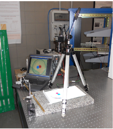
Figure 1: (Color online) The experimental set up. The camera is suspended above the Petri dish and the system is illuminated from below by a light emitting capacitor. The simultaneous insertion of the two drops is carried out with a mechanical rod which holds two graduated injectors together. This device allows for the change of the distance between the drops at will, and in a completely reproducible fashion.

IV Diffusion of one isolated drop

The simplest situation, and the one which we used to calibrate parameters associated with the ink, was when one isolated drop was allowed to form within the Petri dish diff_ink . The ink was injected at one specific location; varying the amount of material that was introduced did not alter the fact that it formed into a regular, almost two dimensional, circular domain. The region of interest in the recorded image was then cropped, and the operation repeated for all successive snapshots of the dynamics, resulting in the gallery of images displayed in Fig. 2. A movie of the dynamics of the drop is attached as supplementary material.

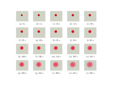
Figure 2: (Color online) Magenta drop: a gallery of images (a)-(t) is displayed at different times covering 495s with acquisition step of 5s. The images are treated so as to isolate the region of interest where the drop is localized. The experiments are carried out at a temperature of $17\pm 1^{o}C$.

The photographs that were obtained were then processed using the freely available ImageJ software Image . Depending on the color of the ink, a specific filter was chosen, which maximized the corresponding adsorption and so enhanced the contrast of the drop. Thus, the green channel was employed when analyzing the magenta signal, while the red channel was used for the cyan drop. This choice simply follows from the subtractive theory of the CMYK color model CMYK .

Each image, converted into an intensity matrix, was normalized to the value of the maximum and then expressed in binary form. This was carried out by choosing a given (arbitrary — see later discussion) threshold and setting pixels with an intensity lower than this threshold to 0, and those with an intensity above this threshold to 1. Each binary map was filtered to eliminate isolated pixels and small spurious features.

From this set of binary images, the diameter $d_{m}$ of the circular profile corresponding to the magenta drop was determined. For definiteness, we shall focus on the magenta drop to describe the procedure; the subscript $m$ denotes magenta. The data are plotted as magenta colored circles in Fig. 3. This quantifies the growth of the drop, which was qualitatively displayed using the raw data in Fig. 2. In Fig. 3, the vertical axis is $d_{m}$, expressed in pixels. The conversion from pixels to physical units is straightforward, provided the resolution of the camera used is known (see caption of Fig. 3).

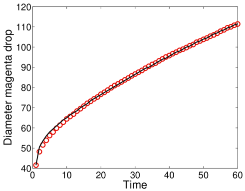
Figure 3: (Color online) The diameter $d_{m}$ of the magenta drop plotted versus time. The diameter is expressed in pixels ($1$ pixel $\simeq$ $0.33$mm). Snapshots are taken every 5s. Symbols refer to the experimental data, the diameter of the drops being calculated via an automatic procedure which transforms the two-dimensional intensity plot into a binary matrix. The solid line represents the solution of Eq. (2), where the diffusion coefficient $D_{m}$ and the relative threshold $\gamma_{m}$ are adjusted via a least square fitting procedure that maximizes the agreement between theory and experiments. In the simulations, at $t=0$, the drop is assumed to uniformly occupy a circular area. The radius of the circle (in pixels) is assigned so as to approximately match the size of the drop as seen in the first of the available experimental images. The simulations are performed over a square domain $L\times L$, with $L=150$ pixels. The best fit values are $D_{m}=0.7712$ pixels²s^-1 and $\gamma_{m}=0.0675$.

We hypothesise that the observed dynamics is purely diffusive diff_ink . Motivated by this belief, we seek to establish a direct connection between the experimental data points, as displayed in Fig. 3, and Eq. (2), which governs the dynamics of diffusive processes. It is worth emphasising that Eq. (2) governs the time evolution of the density of the diffusing species, while the experimental points recorded are calculated from intensity signals as registered by the camera. Comparison of the profiles from the equation and from the data is therefore not straightforward, since the transformation from intensities to densities is highly non-linear. It is possible, however, to make a comparison at the level of the (circular) domain obtained from data in the manner described above. The idea is to numerically integrate Eq. (2) with the diffusion coefficient $D$ (here identified as $D_{m}$) being adjusted iteratively so as to maximize the agreement between the theoretical and experimental curves. This is not the only free parameter: recall that the threshold imposed when performing the binary conversion was arbitrarily chosen. Once again, the transformation between that threshold parameter and the one which delimits the boundary of the drop in the numerical integrations of the equation will be highly non-linear. However, we do not need to characterize this mapping, and need only know that there is a one-to-one correspondence between them, using the threshold parameter in the numerical integrations as the other free parameter of the theory. We denote it by $\gamma_{m}$. Therefore the numerical solution of Eq. (2) will contain two free parameters: $D_{m}$ and $\gamma_{m}$.

We have referred to the solution of Eq. (2) as obtained from a numerical integration. It is, of course, possible to solve Eq. (2) analytically, but we choose to find the solution numerically because we wish to use the same method in the case of two drops, and to test the methodology in the present case of a single drop. Since the corresponding Eqs. (8) are not exactly solvable, we are forced in the case of two drops to use numerical integration methods.

The procedure is now that defined above: to iteratively adjust the two parameters $D_{m}$ and $\gamma_{m}$ so as to maximize the agreement between the theoretical and experimental curves. However, the experimental data gives the radius $d_{m}$ of the circular domain, and we need to relate this to $\gamma_{m}$. We choose to do this as follows: if the drop extends over a two-dimensional circular domain of radius $d_{m}$, then $\phi(x,y,t)/{\textrm{max}}_{x,y}(\phi(x,y,t))<\gamma_{m}$ for each point $\mathbf{x}=(x,y)$ in the domain.

The experimental data, represented by circles, are plotted as function of time in Fig. 3. The solid line represents the solution of the diffusion equation (2), with the diffusion constant $D_{m}$ and the threshold parameter $\gamma_{m}$ found using the iterative fitting scheme described above. The agreement is excellent, the evolution of the drop being, as expected, purely diffusive. Similar conclusions can be reached for the cyan drop. Experimental and theoretical computed diameters $d_{c}$ are compared in Fig. 4. The diffusion constant $D_{c}$ and the threshold $\gamma_{c}$ for cyan are found by analogy with that for magenta, that is, through the iterative fitting procedure described above.

We conclude that standard diffusion theory adequately explains the dynamics of isolated drops, as seen in the experiments that we carried out. A straightforward fitting strategy allowed us to calculate the associated diffusion constants for the two different colors of ink that we studied. These values will be assumed, and used as input, in the more complex scenario where two drops simultaneously evolve in the same Petri dish. We now go on to discuss the corresponding analysis in this case.

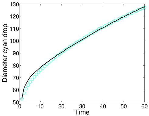
Figure 4: (Color online) The diameter $d_{c}$ of the cyan drop plotted against time. Symbols represent experimental data. The solid line represents the solution of Eq. (2), where the diffusion coefficient $D_{c}$ and the threshold parameter $\gamma_{c}$ are found via a fitting procedure. The initial condition in the simulations is set as described in the caption of Fig. 3. The best fit values are $D_{c}=0.9459$ pixels²s^-1 and $\gamma_{c}=0.0628$.

V Diffusion of two drops: mutual interference and cross terms

In this Section we discuss the diffusion of two ink drops, one magenta and the other cyan, which were simultaneously inserted into the Petri dish described above. The drops were initially localized in different parts of the dish, and so did not influence each other. Diffusion made them gradually expand, until they eventually came into contact, as shown in Fig. 5. At this point, a sharp interface developed between the drops which acted as a barrier preventing the mixing of the two compounds. From then on, the constraints imposed by this barrier distorted the previously circular profiles, as shown in Fig. 6. We interpret this phenomenon as stemming from the competition of the molecular constituents for the finite available space. The saturation of microscopic spatial resources presumably results in locally congested configurations, that are responsible for the macroscopic features seen in experiments.

To test this hypothesis we proceeded as follows. We defined an $X$-axis as the direction of the line connecting the centers of mass of the two drops at $t=0$. A $Y$-axis was then defined as being orthogonal to the $X$-axis. The images recorded were then processed to measure the maximal extension of both of the drops, along the two independent directions $X$ and $Y$, at different times of acquisition of the signal. This therefore gave four quantities at each time $t$, two for the magenta drop and two for the cyan drop. The values obtained were found by filtering the recorded intensity map with an imposed threshold, following the strategy discussed above. This created a binary representation of the two drops, the analysis returning four time series, two for each drop. The data are plotted in Fig. 7: the upper panel displays the data corresponding to the magenta drop, the lower panel to the cyan drop. In both panels, the circles represent the measurements carried out along the $Y$ direction, perpendicular to the line connecting the centers of mass of the drops. The squares refer to the extension of the drops in the $X$ direction, along the line connecting the centers of mass.

The initial condition used in solving Eqs. (8) mimics that found in the experiment. The drops, assumed to be approximately circular at $t=0$, are in fact assigned a specific size that is deduced from the experiments — from the first of the recorded images. Similarly, the relative separation between the drops is calculated in pixels and used as an input to the numerical simulations.

At relatively short times, before the magenta and cyan drops come into contact, their diameters in the $X$ and $Y$ directions are approximately the same, their shape being approximately circular. As already remarked, once the fronts collide ($t\simeq 100s$, see Figs. 5 and 6 panel $(m)$), the dynamics slows down at the interface of the two drops. The merging of the drops is consequently impeded along the direction of collision, a dynamical effect that contributes to reducing the growth of the drop width along the $X$ direction. By contrast, the diameter of both drops keeps on increasing along the $Y$ direction as if normal diffusion governed the dynamics. The symmetry of the system is therefore broken, as clearly shown in Fig. 7.

To establish a bridge between the results of the experiments and the multispecies model of diffusion (8), we used a fitting protocol based on the analysis developed in Sec. IV. In particular, the coefficients $D^{(1)}\equiv D_{c}$ and $D^{(2)}\equiv D_{m}$ are obtained from the single drop analysis, as are the respective thresholds $\gamma_{c}$ and $\gamma_{m}$. Two parameters are left undetermined, the rescaled normalization constants $\bar{\phi^{(1)}}$ and $\bar{\phi^{(2)}}$. These will serve as fitting parameters, found by optimizing the agreement between theory and measurements. The difference between the two, that is minimized by the iterative fitting scheme, is the sum of the norm of relative deviations between the numerically computed and the experimentally measured diameters, along the two directions of observation, for both drops, at the same time. It should be emphasised that, due to the nonlinearity introduced by the cross terms in Eq. (8), the normalization factors $\bar{\phi^{(1)}}$ and $\bar{\phi^{(2)}}$ do not trivially cancel, as is the case if the linear diffusion equation (2) is assumed to govern the dynamics. Larger values of $\bar{\phi^{(1)}}$ and $\bar{\phi^{(2)}}$, enhance the impact of cross terms and so magnify the deviations from the purely diffusive scenario.

While $\bar{\phi^{(1)}}$ and $\bar{\phi^{(2)}}$ indirectly quantify the amount of material that was introduced into the Petri dish, they are also probably sensitive to the microscopic shape and steric properties of individual ink molecules, supposedly distinct for cyan and magenta samples. Moreover, $\bar{\phi^{(1)}}$ and $\bar{\phi^{(2)}}$ may encapsulate three-dimensional effects, which although assumed to be negligible in our treatment, are responsible for a slight deformation of the drops along the vertical, $z$ direction, an effect which, a priori, is different for the two drops. Based on these considerations, and despite the fact that care has been taken to keep the two drops as similar as possible at the time of injection into the dish, one should allow for different values of the unknown constants $\bar{\phi^{(1)}}$ and $\bar{\phi^{(2)}}$.

The result of the fitting procedure is reported in Fig. 7. The fitting is first performed by only adjusting the average number densities $\bar{\phi}^{(1)}$ and $\bar{\phi}^{(2)}$; here cyan is the molecular species $1$ and magenta the molecular species $2$. The diffusivities, $D_{c}$ and $D_{m}$, as well as the thresholds, $\gamma_{c}$ and $\gamma_{m}$, are set to the values determined above when analyzing the single drop dynamics (see captions of Figs. 3 and 4). The time series for the widths of the two drops (a total of four independent curves) are hence simultaneously fitted by using only two control parameters. The best fit values are $\bar{\phi}^{(1)}=0.3406$ and $\bar{\phi}^{(2)}=0.2126$.

The dashed lines in Fig. 7 are the result of a generalized fitting strategy, where the thresholds $\gamma_{m}$ and $\gamma_{c}$ are also allowed to vary. In this latter case, the fitted parameters result in $\bar{\phi}^{(1)}=0.32815$, $\bar{\phi}^{(2)}=0.2233$, $\gamma_{m}=0.0727$ and $\gamma_{c}=0.0608$. In the case of the cyan drop, shown in the lower panel of Fig. 7, the dashed lines obtained from the generalized fitting strategy which uses four free parameters are not distinguishable from the solid lines, obtained when only two free parameters are used.

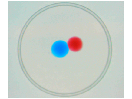
Figure 5: (Color online) The two drops in the Petri dish, some time after injection.

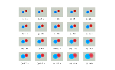
Figure 6: (Color online) A collection of images displaying the dynamics of the two drops at different times. The images cover a window of observation of 295s, with an acquisition step of 5s. A movie of the time evolution of the two drops is annexed as supplementary material.

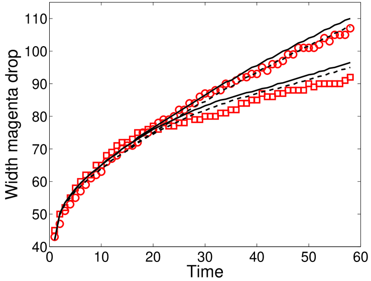
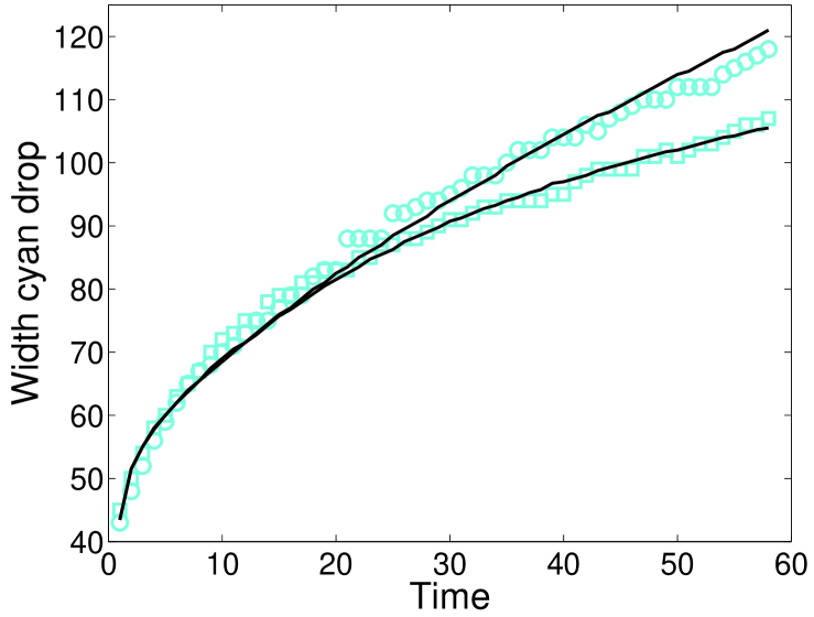
Figure 7: (Color online) Upper panel: The diameters of the magenta drop are displayed versus time. Symbols refer to the experiments: open circles for the diameter of the drop in the $Y$ direction and squares for the diameters along $X$. The solid lines represent the numerical fit based on the generalized diffusion Eqs. (8). The dashed lines are the result of a generalized fitting strategy, described in the main text. Lower panel: As for the upper panel, but for the cyan drop. The simulations are performed over a square of linear size $L$, with $L=150$.

In summary, by adjusting two fitting parameters we are able to approximate four curves, representing the time evolution of the widths of the two drops along the reference directions $X$ and $Y$, with good accuracy. The slight deviation observed for the magenta drop is partially removed by allowing for the thresholds to change by a few percent, with respect to the values determined for the single drop case. The fact that $\gamma_{m}$ is modified by the generalized fitting strategy has its origins in a cross-talk between color channels. The cyan drop induces a small offset in the magenta channel, when the two drops are present simultaneously in the analyzed image. This effect is responsible for the small change in $\gamma_{m}$, as compared to the value obtained for an isolated magenta drop.

The results obtained point to the validity of the model of multispecies diffusion described in Sec. II. The model is capable of mimicking the mutual interference between different chemical compounds confined to the same spatial reservoir, under crowded conditions, as seen in the experiments reported here.

VI Conclusion

The problem of multispecies diffusion is of great importance in many areas of science. Particularly crucial is the field of biology, where distinct molecular constituents, organized in families, populate (for instance) the cellular medium under crowded conditions. Among the models that have been proposed in the literature to analyze diffusion in a multi-component system, the one derived in FanelliMckane moves from a microscopic, hence inherently stochastic formulation of the problem, to macroscopic equations which incorporate the consequences of crowding. It does this by accounting for the effect of limited spatial resources, that seed an indirect competition between the different molecular species. The model of FanelliMckane therefore comprises of a set of (deterministic) differential equations which are fully justified from first principles, and which are also expected to apply in situations when large densities are present. In this paper we have tested this model experimentally by investigating the diffusion of two ink drops which are simultaneously evolving in a container filled with water.

The experimental set up was calibrated with reference to the single drop case study, a simplified scenario that enabled us to measure the characteristic diffusion coefficients of the ink. When instead two drops are introduced into the container, a curious phenomenon takes place: after an initial evolution, which can be explained using the standard theory of diffusion, the fronts of the drops collide and a barrier is established at the interface which prevents mixing of the ink drops. This observation cannot be described by normal diffusion theory. The symmetry between the $X$ and $Y$ directions (defined respectively to be the direction of the impact and that orthogonal to it) is in fact broken, an intriguing dynamical feature that we interpret as the macroscopic consequence of the competition for the microscopic spatial resources that takes place at the frontier between the two drops. To test the model proposed in FanelliMckane we have measured the widths of the drops, along the two independent $X$ and $Y$ directions and compared the experimental data points obtained to the numerical solution of the governing differential equations (8). The numerical time series are compared to the experiments by performing a constrained fitting, which employs a limited number of free parameters. The fitting algorithm incorporates information from an independent and preliminary analysis of the evolution of isolated ink drops in a similar environment. The agreement between theory and experiments is good, pointing to the validity of the mathematical model derived in FanelliMckane . We therefore conclude that this model accurately captures the dynamics of two, simultaneously diffusing, granular species, in the non-trivial situation where crowding occurs.

The results of the experiments reported in this paper, together with the derivation of the model and its numerical and analytical study, lead us to propose that it should be adopted in reaction-diffusion problems, where species are known to be spatially dense, so abandoning the inappropriate Fickean approximation. This allows novel insights to be gained into several important mechanisms, for example Turing instabilities turing1952 and the paradigmatic approach to pattern formation in biology murray . In fanelliciancidipatti ; kumar2011 it is shown that, due to non-Fickean cross-diffusion terms, the Turing instability also sets in when the activator diffuses faster then the inhibitor, at odds with the conventional, currently accepted, picture. We expect many other applications of this microscopically motivated approach to crowding will be explored in the future.

- (1) J. Crank, The Mathematics of Diffusion (OUP, Oxford, 1975). Second edition.
- (2) A. Einstein, Annalen der Physik 17, 549 (1905); A. Einstein Investigations on the Theory of Brownian Movement (Dover, New York, 1956).
- (3) M. Smoluchowski, Annalen der Physik 21, 756 (1906).
- (4) R. Brown, Phil. Mag. 4, 161 (1828).
- (5) J. P. Bouchaud and A. Georges, Phys. Rep. 195, 127 (1990).
- (6) R. Metzler and J. Klafter, Phys. Rep. 339, 1 (2000).
- (7) G. M. Zaslavsky, Phys. Rep. 371, 461 (2002).
- (8) M. Weiss et al., Biophys. J. 87, 3518 (2004).
- (9) D. S. Banks and C. Fradin, Biophys. J. 89, 2960 (2005).
- (10) J. A. Dix and A. S. Verkman, Annu. Rev. Biophys. 37, 247 (2008)
- (11) E. Marcos, P. Mestres and R. Crehuet, Biophys. J 101, 2782 (2011).
- (12) D. Ben-Avraham and S. Havlin. Diffusion and Reactions in Fractals and Disordered Systems (CUP, Cambridge, 2000).
- (13) D. Fanelli and A. J. McKane, Phys. Rev. E 82, 021113 (2010).
- (14) T. Biancalani, D. Fanelli and F. Di Patti, Phys. Rev E 81 046215 (2010).
- (15) D. Fanelli, C. Cianci and F. Di Patti, submitted to Phys. Rev. E (2012) arXiv:1112.0870.
- (16) K. A. Landman and A. E. Fernando, Physica A 390, 3742 (2011).
- (17) N. G. van Kampen, Stochastic Processes in Physics and Chemistry, (Elsevier, Amsterdam, 1992).
- (18) A. J. McKane and T. J. Newman, Phys. Rev E 70, 041902 (2004).
- (19) L. Brugnano and V. Casulli, SIAM Sci. Comp. 30, 463 (2008).
- (20) S. Lee, H-Y Lee, I-F Lee and C-Y Tseng, Eur. J. Phys. 25, 331 (2004).
- (21) Ceelite, Colmar, Pennsylvania (US) (http://www.ceelite.com/ ).
- (22) www.continua-light.com
- (23) The Imaging Source, Bremen, Germany (http://www.theimagingsource.com)
- (24) Royal Talens di Apeldoorn, The Netherlands (http://www.talens.com).
- (25) ImageJ software, http://rsbweb.nih.gov/ij/
- (26) M. Galer and L. Horvat, Digital Imaging: Essential Skills. (Elsevier/Focal Press, Amsterdam, 2003).
- (27) A. M. Turing, Phils. Trans. R. Soc. London Ser. B 237, 37 (1952).
- (28) J.D. Murray, Mathematical Biology (Springer, Berlin, 1989).
- (29) N. Kumar and W. Horsthemke, Phys. Rev. E 83, 036105 (2011).