Low Mach number effect in simulation of high Mach number flow

Abstract

In this note, we relate the two well-known difficulties of Godunov schemes: the carbuncle phenomena in simulating high Mach number flow, and the inaccurate pressure profile in simulating low Mach number flow. We introduced two simple low-Mach-number modifications for the classical Roe flux to decrease the difference between the acoustic and advection contributions of the numerical dissipation. While the first modification increases the local numerical dissipation, the second decreases it. The numerical tests on the double-Mach reflection problem show that both modifications eliminate the kinked Mach stem suffered by the original flux. These results suggest that, other than insufficient numerical dissipation near the shock front, the carbuncle phenomena is strongly relevant to the non-comparable acoustic and advection contributions of the numerical dissipation produced by Godunov schemes due to the low Mach number effect.

and

1 Introduction

In the last decades, Godunov schemes are among the most successful methods in simulating compressible flows involving shock waves and discontinuities [18]. Godunov schemes utilize the solution of an Riemann solver at the face of computational cells as the numerical flux to introduce sufficient numerical dissipation [5]. However, some low-dissipation Godunov schemes, such as those with Roe flux, may suffer from numerical instabilities at the strong shock front, known as the carbuncle phenomena, when simulating multi-dimensional high Mach number flows [15]. Although has not being fully understood, it is generally believed that this problem is caused by the insufficient numerical dissipation near the shock front [15, 16, 20, 11, 8]. Therefore, up to now, almost all the cures proposed for Godunov schemes is trying to increase the numerical dissipation in the near shock-front region, or in the entire computational domain [9, 14, 10, 7].

In this short note, we propose to relate this problem to another well-known difficulty of Godunov schemes in the low Mach number limit [4, 3, 2] . The reason for this connection is that: for a shock wave in the solution of a multi-dimensional high Mach number flow, if it propagates in one direction of the Cartesian, or nearly Cartesian grid, the disturbances parallel to, especially behind, the front propagate in a low Mach number fashion. Actually, the alignment of shock front to the grid is one of the typical scenarios of the carbuncle phenomena [16, 13, 14].

2 Roe flux and its low Mach number modifications

For simplicity, we consider two-dimensional Euler compressible equation

$$\frac{\partial\mathbf{U}}{\partial t}+\frac{\partial\mathbf{F}(\mathbf{U})}{\partial x}+\frac{\partial\mathbf{G}(\mathbf{U})}{\partial y}=0.$$ (1)

where $\mathbf{U}=(\rho,\rho u,\rho v,E)^{T}$, $\mathbf{F}(\mathbf{U})=[\rho u,\rho u^{2}+p,\rho uv,(E+p)u]^{T}$ and $\mathbf{G}(\mathbf{U})=[\rho v,\rho vu,\rho v^{2}+p,(E+p)v]^{T}$. This set of equations describes the conservation laws for mass density $\rho$, momentum density $\rho\mathbf{v}=(\rho u,\rho v)$ and total energy density $E=\rho e+\rho\mathbf{v}^{2}/2$, where $e$ is the internal energy per unit mass. To close this set of equations, the ideal-gas equation of state $p=(\gamma-1)\rho e$ with constant $\gamma$ is used.

The classical Roe flux gives the following form of numerical flux

$$\mathbf{F}_{i+1/2}=\frac{1}{2}\left(\mathbf{F}_{i+1}+\mathbf{F}_{i}\right)-\frac{1}{2}\mathbf{R}_{i+1/2}|\mathbf{\Lambda}_{i+1/2}|\mathbf{R}^{-1}_{i+1/2}(\mathbf{U}_{i+1}-\mathbf{U}_{i}),$$ (2)

where $\mathbf{R}$ and $\mathbf{R}^{-1}$ are the right and left eigenvector matrices of $\partial\mathbf{F}/\partial\mathbf{U}$ and $\mathbf{\Lambda}$ the diagonal matrix formed with relevant eigenvalues:

$$\lambda_{1,2}=u,\quad\lambda_{3,4}=u\pm c.$$ (3)

The first term on the right-hand-side of Eq. (2) is the central flux term, and the second term is the dissipative flux term. Since $\mathbf{R}$ and $\mathbf{R}^{-1}$ are only forward and backward coordinate transformations, the dissipative flux is merely dependent on $\mathbf{\Lambda}$, and has two contributions: one is proportional to $|u|$, is called advection dissipation, the other proportional to $|u\pm c|$, is called acoustic dissipation.

The asymptotic analysis on Roe flux and general Godunov schemes [4, 3] show that, when $M\ll 1$, where $M=|u|/c$ is the Mach number, or the acoustic contribution of the numerical dissipation is much larger than that of the advection, the dissipative flux term lead to pressure fluctuations of order $\mathcal{O}(M)$ at the cell face even if the initial data are well-prepared and contain only pressure disturbances of order $\mathcal{O}(M^{2})$. This phenomenon on inaccurate prediction of pressure profile is called low Mach number effect. One straightforward way to decrease the low Mach number effect is increasing the value of $M$ in $\mathbf{\Lambda}$ to obtain comparable acoustic and advection contributions. This leads to two simple modifications of $\mathbf{\Lambda}$ to $\mathbf{\Lambda}^{\prime}$

$$\lambda^{\prime}_{1,2}=u,\quad\lambda^{\prime}_{3,4}=u\pm\min(\phi|u|,c),$$ (4)

and to $\mathbf{\Lambda}^{\prime\prime}$

$$\lambda^{\prime\prime}_{1,2}=u^{\prime\prime},\quad\lambda^{\prime\prime}_{3,4}=u^{\prime\prime}\pm c,\quad u^{\prime\prime}={\rm sgn}(u)\max\left[\frac{c}{\phi},|u|\right],$$ (5)

where $\phi$ is a positive number of order $\mathcal{O}(1)$. The Roe flux with Eq. (4) is denoted as Roe-M1 and with Eq. (5) as Roe-M2. Unlike Guillard and Viozat [4] and Li et al. [12], these modifications do not change the eigenvector matrix or the central flux term. Note that, though both modifications lead to comparable acoustic and advection contributions of numerical dissipation in the low Mach number region or direction of the flow, while the Roe-M1 flux decreases the local numerical dissipation, the Roe-M2 flux increases it.

3 Simulation and discussion

We test the calssical Roe, Roe-M1 and Roe-M2 fluxes, with $\phi=5$, for a problem from Woodward and Colella [19] on the double Mach reflection of a Mach 10 shock in air. The initial conditions are

$$(\rho,u,v,p)=\cases{(1.4,0,0,1)&if $y<1.732(x-0.1667)$\\ \cr(8,7.145,-4.125,116.8333)&else\\ },$$

and the final time is $t=0.2$. The computational domain of this problem is $[0,0]\times[4,1]$. Initially, the shock extends from the point $x=0.1667$ at the bottom to the top of the computational domain. Along the bottom boundary, at $y=0$, the region from $x=0$ to $x=0.1667$ is always assigned post-shock conditions, whereas a reflecting wall condition is set from $x=0.1667$ to $x=4$. Inflow and outflow boundary conditions are applied at the left and right ends of the domain, respectively. The values at the top boundary are set to describe the exact motion of a Mach 10 shock. The calculations are carried out with the 5th-order WENO-Z [1] scheme, in which the Roe approximation is used for the characteristic decomposition at the cell faces and the 3rd-order TVD Runge-Kutta scheme is used for time integration [17]. Note that, in order to exclude the influence of entropy condition [11, 8], no entropy fix is used in the computations.

Figure 1 shows the density contours of the solution on a $480\times 120$ grid at $t=0.2$. Note that, a positivity-preserving scheme [6] is implemented to obtain numerically stable results for the classical Roe flux.

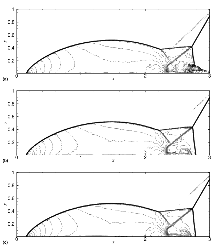
Figure 1: Double-Mach reflection of a Mach 10 shock wave: 40 density contours from 1.88783 to 20.9144 at $t=0.2$, on a $480\times 120$ grid with the (a) classical Roe, (b) Roe-M1, and (c) Roe-M2 fluxes.

It is observed that, contrast to that the classical Roe flux suffers from a kinked Mach stem, a typical configuration of the carbuncle phenomena, both Roe-M1 and Roe-M2 fluxes produce numerically stable and correct results. While Roe-M2 flux eliminates the kinked Mach stem by introducing extra advection dissipation parallel to the shock front, Roe-M1 flux achieves this by decreasing acoustic dissipation. Note that, since Roe-M1 decreases the overall local numerical dissipation near the shock front, it is unlikely that the kinked Mach stem is produced due to insufficient numerical dissipation. Further numerical experiments show that, if the numerical dissipation is modified by only increasing the value of $c$ in Eq. (3) i.e. only the acoustic dissipation increased, the simulation still suffers from the kinked Mach stem (not shown here). All these results clearly suggest that the carbuncle phenomena is strongly relevant to the non-comparable acoustic and advection contributions of the numerical dissipation produced by Godunov schemes due to the low Mach number effect.

References

- [1] R. Borges, M. Carmona, B. Costa, and W.S. Don. An improved weighted essentially non-oscillatory scheme for hyperbolic conservation laws. J. Comput. Phys., 227(6):3191–3211, 2008.
- [2] S. Dellacherie. Analysis of godunov type schemes applied to the compressible euler system at low mach number. J. Comput. Phys., 229(4):978–1016, 2010.
- [3] H. Guillard and A. Murrone. On the behavior of upwind schemes in the low mach number limit: Ii. godunov type schemes. Computers & fluids, 33(4):655–675, 2004.
- [4] H. Guillard and C. Viozat. On the behaviour of upwind schemes in the low mach number limit. Computers & fluids, 28(1):63–86, 1999.
- [5] A. Harten, P.D. Lax, and B. Van Leer. On upstream differencing and godunov-type schemes for hyperbolic conservation laws. SIAM review, pages 35–61, 1983.
- [6] X.Y. Hu and N.A. Adams. A positivity-preserving flux limiter for high order conservative schemes. arXiv:1203.1540.
- [7] K. Huang, H. Wu, H. Yu, and D. Yan. Cures for numerical shock instability in hllc solver. Int. J. Numer. Meth Fluid, 65(9):1026–1038, 2011.
- [8] F. Ismail and P.L. Roe. Affordable, entropy-consistent euler flux functions ii: Entropy production at shocks. J. Comput. Phys., 228(15):5410–5436, 2009.
- [9] S. Kim, C. Kim, O.H. Rho, and S. Kyu Hong. Cures for the shock instability: development of a shock-stable roe scheme. J. Comput. Phys., 185(2):342–374, 2003.
- [10] S.D. Kim, B.J. Lee, H.J. Lee, and I.S. Jeung. Robust hllc riemann solver with weighted average flux scheme for strong shock. J. Comput. Phys., 228(20):7634–7642, 2009.
- [11] K. Kitamura, P. Roe, and F. Ismail. Evaluation of euler fluxes for hypersonic flow computations. AIAA Journal, 47(1):44–53, 2009.
- [12] X. Li, C. Gu, and J. Xu. Development of roe-type scheme for all-speed flows based on preconditioning method. Computers & Fluids, 38(4):810–817, 2009.
- [13] M.S. Liou. Mass flux schemes and connection to shock instability. J. Comput. Phys., 160(2):623–648, 2000.
- [14] H. Nishikawa and K. Kitamura. Very simple, carbuncle-free, boundary-layer-resolving, rotated-hybrid riemann solvers. J. Comput. Phys., 227(4):2560–2581, 2008.
- [15] J.J. Quirk. A contribution to the great riemann solver debate. Int. J. Numer. Meth Fluid, 18(6):555–574, 1994.
- [16] R. Sanders, E. Morano, and M.C. Druguet. Multidimensional dissipation for upwind schemes: stability and applications to gas dynamics. J. Comput. Phys., 145(2):511–537, 1998.
- [17] C.W. Shu and S. Osher. Efficient implementation of essentially non-oscillatory shock-capturing schemes. J. Comput. Phys., 77(2):439–471, 1988.
- [18] E.F. Toro. Riemann solvers and numerical methods for fluid dynamics: a practical introduction. Springer Verlag, 2009.
- [19] P. Woodward and P. Colella. The numerical simulation of two-dimensional fluid flow with strong shocks. J. Comput. Phys., 54(1):115–173, 1984.
- [20] K. Xu and Z. Li. Dissipative mechanism in godunov-type schemes. Int. J. Numer. Meth Fluid, 37(1):1–22, 2001.