Series solution to the first-passage-time problem of a Brownian motion with an exponential time-dependent drift

Abstract

We derive the first-passage-time statistics of a Brownian motion driven by an exponential time-dependent drift up to a threshold. This process corresponds to the signal integration in a simple neuronal model supplemented with an adaptation-like current and reaching the threshold for the first time represents the condition for declaring a spike. Based on the backward Fokker-Planck formulation, we consider the survival probability of this process in a domain restricted by an absorbent boundary. The solution is given as an expansion in terms of the intensity of the time-dependent drift, which results in an infinite set of recurrence equations. We explicitly obtain the complete solution by solving each term in the expansion in a recursive scheme. From the survival probability, we evaluate the first-passage-time statistics, which itself preserves the series structure. We then compare theoretical results with data extracted from numerical simulations of the associated dynamical system, and show that the analytical description is appropriate whenever the series is truncated in an adequate order.

1 Introduction

The statistical analysis of a system is essential when fluctuations contribute to its dynamics [1, 2, 3]. In different areas, beyond the importance of the statistical description of the system state and its evolution, the main variable of interest is the time at which this state reaches a certain region for the first time [4], constituting the so-called first-passage-time (FPT) problem. For example, in a diffusion-controlled reaction a particle performs a random walk until it makes contact with a reactant or a trap giving rise to the reaction [4]. Generally, in a FPT problem, the system is able to evolve according to a given dynamics in a confined region, limited by one or more absorbing boundaries. Even for simple autonomous systems, the FPT problem can be analytically difficult to solve. For example, for the Ornstein-Uhlenbeck process with a fixed positive absorbing boundary, the FPT solution (representing the FPT density function) is relatively easy to be found in the Laplace domain, but its inverse transform is not explicitly available [5]. A notable exception is the FPT problem for a Brownian motion (Wiener process), where different methods are easy to be applied to solve it [1, 2, 4, 5, 6]. A greater complexity is found when a time-inhomogeneous process defines the system dynamics. In this case, analytical methods are formally given within different approaches [2, 4, 5, 7, 8], but exact as well as approximate explicit results are scarce in the literature and probably difficult to obtain. Among the different ways to introduce a time inhomogeneity into the system (for example, temporally varying absorbing boundaries [9, 10], time-dependent drift and diffusion coefficients [11], etc), we focus on a particular drift coefficient evolving externally in time. The process analysed here is driven by an exponential time-dependent drift (this case, in turn, can be mapped into a variable threshold [9]), which naturally arises in neuroscience when modelling adapting neurons [12, 13, 14, 15, 16, 17]. In this context, the membrane potential (state variable) of a perfect integrate-and-fire neuron model is driven during its subthreshold evolution by an external current, composed of a constant deterministic current plus fast fluctuations [2, 5, 6, 18, 19], as well as an intrinsic temporally decaying current [17, 20]. This system corresponds exactly to the case analysed here, and the FPT represents the production of a spike.
The interest in the FPT problem for a Brownian particle in a time-inhomogeneous setup started in the 1990s, when different systems driven by periodically modulated drifts were studied within the context of the stochastic resonance phenomenon [21]. In particular, Bulsara et al applied the method of images to a Wiener process driven by a sinusoidal temporal drift in the presence of an absorbing boundary [22], a procedure of limited validity [23, 24, 11]. Later, other threshold processes under analogous conditions were theoretically analysed with different approximation methods [21, 25, 26, 27]. Even when appealing, single sinusoidal temporal drifts do not represent a general case. For arbitrary time-dependent drifts, the simplest procedures are a quasiadiabatic reduction [28], a quasistatic description [29], or small amplitude approximations. However, for rapidly varying arbitrary fields, the time-dependent structure of the problem cannot be simplified. Up to our knowledge, the first attempt to include an arbitrary temporal drift (without spatial dependence) in a general framework was made in [30], where the author proposed a method to describe the first-order correction to the moments of the FPT density, in a perturbation scheme.
The preceding studies describe approximately the FPT problem of a given continuous stochastic process in a restricted domain for particular or general temporal drifts. In general, explicit exact results for time-inhomogeneous systems are infrequent. Notably and as an exception, in [11] the authors derive the FPT density function of a Wiener process, in the presence of an absorbing boundary, where both the drift and the diffusion coefficients are varying temporally and in proportion to each other. In particular, when proportionality is satisfied, the Fokker-Planck equation ruling the evolution of the transition probability between the states at two times can be time-rescaled in order to resemble the simpler constant coefficients case, where the exact solution is known. However, the restriction in the coefficients proportionality limits its applicability to our case. For the FPT problem we are interested in, we have previously proposed a series solution in terms of the intensity of the time-dependent drift [31] (see also [23, 28] for analogous series solutions, but focusing on the perturbation regime). However, in that work only the first terms in the expansion were explicitly given and higher order terms were just outlined.
In this work, based on the structure of the equations obtained in [31] for the survival probability, we explicitly obtain all order functions. In particular, we find the $n$th-term in a recursive scheme and prove by induction the complete mathematical solution. From the survival probability, it is straightforward to derive the FPT statistics, which maintains the series structure. Since obtaining all order functions (existence) does not imply the convergence of the series, in the second part of the work, we analyse how does the expansion behave in comparison with results obtained from simulations, as we truncate the series at a finite order.

2 Theoretical framework

In this section, we set the system under analysis, the formalism we use to study the survival probability and the FPT density function, and derive the complete solution.

2.1 The system

The dynamics of the system is governed by the Langevin equation

$$\frac{\rmd x}{\rmd t}=\mu+\frac{\epsilon}{\tau_{\rm d}}\rme^{-(t-t_{0})/\tau_{\rm d}}+\xi(t),$$ (1)

where $x$ is the state variable (e.g. particle position, membrane potential, etc), $t$ is the time, $\mu$ is the constant (positive) component of the drift, $\epsilon$ and $\tau_{\rm d}$ characterize the intensity and the time constant of the exponential time-dependent drift, respectively, $t_{0}$ sets the initial time and $\xi(t)$ is a Gaussian white noise with (constant) squared intensity $D$ [$\langle\xi(t)\rangle=0$ and $\langle\xi(t)\xi(t^{\prime})\rangle=2D\delta(t-t^{\prime})$].
Following the derivation we have made in [31], the probability that the particle remains in the domain $x<x_{\rm thr}$ at time $t^{\prime}$, given the (variable) initial condition $x$ at (variable) time $t$, $F(t^{\prime}|x,t)$, evolves according to the backward FP equation

$$\frac{\partial F(t^{\prime}|x,t)}{\partial t}=-\left[\mu+\frac{\epsilon}{\tau_{\rm d}}~{}\rme^{-(t-t_{0})/\tau_{\rm d}}\right]\frac{\partial F(t^{\prime}|x,t)}{\partial x}-D~{}\frac{\partial^{2}F(t^{\prime}|x,t)}{\partial x^{2}}.$$ (2)

In Eq. (2), $t^{\prime}$ is a parameter accounting for the present time. By making the substitution $\tau=t^{\prime}-t$ and renaming the probability as $F(x,\tau;t^{\prime})$, Eq. (2) can be written as

$$\frac{\partial F(x,\tau;t^{\prime})}{\partial\tau}=\left[\mu+\frac{\epsilon}{\tau_{\rm d}}~{}\rme^{-(t^{\prime}-t_{0})/\tau_{\rm d}}~{}\rme^{\tau/\tau_{\rm d}}\right]\frac{\partial F(x,\tau;t^{\prime})}{\partial x}+D~{}\frac{\partial^{2}F(x,\tau;t^{\prime})}{\partial x^{2}},$$ (3)

which represents the equation to be solved. The system is completed by specifying the initial and boundary conditions [31], which are

$$F(x,\tau=0;t^{\prime}) = \cases{1~{}~{}{\rm for}~{}x<x_{\rm thr},\\ 0~{}~{}{\rm for}~{}x\geq x_{\rm thr},}$$ (4)

$$F(x=x_{\rm thr},\tau;t^{\prime}) = 0.$$ (5)

Equation (4) indicates that the survival at initial time is certain for a particle located in the domain of interest, whereas Eq. (5) establishes that the particle is not allowed to be in $x\geq x_{\rm thr}$ and, therefore, $x=x_{\rm thr}$ is an absorbent boundary.
By proposing a solution as an expansion in $\epsilon$,

$$\hskip 14.22636ptF(x,\tau;t^{\prime})=F_{0}(x,\tau;t^{\prime})+\epsilon~{}F_{1}(x,\tau;t^{\prime})+\epsilon^{2}~{}F_{2}(x,\tau;t^{\prime})+\dots=\sum_{n=0}^{\infty}\epsilon^{n}~{}F_{n}(x,\tau;t^{\prime}),$$ (6)

Equation (3) reads

$$\hskip 42.67912pt\left[\frac{\partial F_{0}}{\partial\tau}-\mu\frac{\partial F_{0}}{\partial x}-D\frac{\partial^{2}F_{0}}{\partial x^{2}}\right]$$

$$+\sum_{n=1}^{\infty}\epsilon^{n}~{}\left[\frac{\partial F_{n}}{\partial\tau}-\mu\frac{\partial F_{n}}{\partial x}-\frac{1}{\tau_{\rm d}}~{}\rme^{-(t^{\prime}-t_{0})/\tau_{\rm d}}~{}\rme^{\tau/\tau_{\rm d}}~{}\frac{\partial F_{n-1}}{\partial x}-D\frac{\partial^{2}F_{n}}{\partial x^{2}}\right]=0.$$ (7)

Since we expect that all functions $F_{n}$ do not depend on $\epsilon$, Eq. (6), the expressions between brackets should be identically $0$. Obviously, this hypothesis is true if we are able to find $F_{n}(x,\tau;t^{\prime})$. Under this condition, the complete solution for $F(x,\tau;t^{\prime})$ is given by the system of equations

$$\frac{\partial F_{0}}{\partial\tau}-\mu~{}\frac{\partial F_{0}}{\partial x}-D~{}\frac{\partial^{2}F_{0}}{\partial x^{2}} = 0,$$ (8)

$$\frac{\partial F_{n}}{\partial\tau}-\mu~{}\frac{\partial F_{n}}{\partial x}-D~{}\frac{\partial^{2}F_{n}}{\partial x^{2}} = \frac{1}{\tau_{\rm d}}~{}\rme^{-(t^{\prime}-t_{0})/\tau_{\rm d}}~{}\rme^{\tau/\tau_{\rm d}}~{}\frac{\partial F_{n-1}}{\partial x},~{}~{}{\rm for}~{}~{}n\geq 1.$$ (9)

Consistently with our previous assumption, given the arbitrariness of $\epsilon$, the non-homogeneous initial condition, $F(x,\tau=0;t^{\prime})=1$ for $x<x_{\rm thr}$, should be exclusively imposed to the zeroth-order function $F_{0}(x,\tau=0;t^{\prime})$. In detail, initial conditions are

$$F_{0}(x,\tau=0;t^{\prime}) = \cases{1~{}~{}{\rm if}~{}x<x_{\rm thr},\\ 0~{}~{}{\rm if}~{}x\geq x_{\rm thr},}$$ (10)

$$F_{n}(x,\tau=0;t^{\prime}) = 0~{}~{}{\rm for}~{}n\geq 1.$$ (11)

Completing the description, the boundary condition reads $F_{n}(x=x_{\rm thr},\tau;t^{\prime})=0$, for all $n$.

2.2 Survival probability from the backward state

To obtain exactly the survival probability at time $t^{\prime}$ from the backward state we have to solve all terms involved in the expansion given by Eq. (6). In particular, each term satisfies a certain equation, Eq. (8) or (9), with appropriate conditions. Due to the different mathematical structure, we focus on the zeroth-order term, $F_{0}(x,\tau;t^{\prime})$, separately from all other superior terms, $F_{n}(x,\tau;t^{\prime})$ for $n>0$.

2.2.1 Zeroth-order term.

This term corresponds to the survival probability at time $t^{\prime}$ of a Brownian particle (initially) located in $x$ at time $t$, when the system is driven exclusively by a constant positive drift $\mu$ (in our system, this is obtained with $\epsilon=0$). According to the preceding derivation, $F_{0}(x,\tau;t^{\prime})$ satisfies Eq. (8) with the conditions given by Eq. (10) and $F_{0}(x_{\rm thr},\tau;t^{\prime})=0$. Since $F_{0}(x,\tau;t^{\prime})=0$ for $x\geq x_{\rm thr}$, we focus exclusively on $x<x_{\rm thr}$; in this case, by Laplace transforming Eq. (8), we obtain

$$s~{}\tilde{F}_{0}^{L}(x)-\mu~{}\frac{\rmd\tilde{F}_{0}^{L}(x)}{\rmd x}-D~{}\frac{\rmd^{2}\tilde{F}_{0}^{L}(x)}{\rmd x^{2}}=1,$$ (12)

where $\tilde{F}_{0}^{L}(x,s;t^{\prime})=\int_{0}^{\infty}\rme^{-s\tau}~{}F_{0}(x,\tau;t^{\prime})~{}d\tau$ is the Laplace transform of $F_{0}(x,\tau;t^{\prime})$ in the variable $\tau$. Since $t^{\prime}$ and $s$ act as parameters in Eq. (12), we have simplified the notation to $\tilde{F}_{0}^{L}(x)$. In Laplace domain, the boundary condition simply transforms to $\tilde{F}_{0}^{L}(x_{\rm thr})=0$.
The solution to Eq. (12), with the preceding condition and taking into account that $\tilde{F}_{0}^{L}(x)$ remains bounded as $x\rightarrow-\infty$, is

$$\tilde{F}_{0}^{L}(x)=\frac{1}{s}-\frac{1}{s}~{}\exp\left\{\frac{(x_{\rm thr}-x)}{2D}[\mu-\sqrt{\mu^{2}+4Ds}]\right\}.$$ (13)

The inverse Laplace transform of $\tilde{F}_{0}^{L}(x,s;t^{\prime})$ can be explicitly computed and reads

$$F_{0}(x,\tau;t^{\prime})=1 - \frac{1}{2}~{}{\rm erfc}\Big{[}\frac{(x_{\rm thr}-x)}{2\sqrt{D\tau}}-\frac{\mu}{2}\sqrt{\frac{\tau}{D}}\Big{]}$$ (14)

$$- \frac{1}{2}~{}\exp\Big{[}{\frac{(x_{\rm thr}-x)~{}\mu}{D}}\Big{]}~{}{\rm erfc}\Big{[}\frac{(x_{\rm thr}-x)}{2\sqrt{D\tau}}+\frac{\mu}{2}\sqrt{\frac{\tau}{D}}\Big{]},$$

where ${\rm erfc}(x)$ is the complementary error function.

2.2.2 Higher order terms.

The equation governing the dynamics of the $n$th-order function is given by

$$\frac{\partial F_{n}(x,\tau;t^{\prime})}{\partial\tau}-\mu~{}\frac{\partial F_{n}(x,\tau;t^{\prime})}{\partial x}-D~{}\frac{\partial^{2}F_{n}(x,\tau;t^{\prime})}{\partial x^{2}}=\frac{1}{\tau_{\rm d}}\rme^{-(t^{\prime}-t_{0})/\tau_{\rm d}}~{}\frac{\partial}{\partial x}\left[\rme^{\tau/\tau_{\rm d}}~{}F_{n-1}(x,\tau;t^{\prime})\right],$$ (15)

and the boundary and initial conditions are $F_{n}(x_{\rm thr},\tau;t^{\prime})=0$ and $F_{n}(x,\tau=0;t^{\prime})=0$, respectively.
This equation can be solved via a Laplace transformation in the variable $\tau$, which reads

$$s~{}\tilde{F}_{n}^{L}(x)-\mu~{}\frac{\rmd\tilde{F}_{n}^{L}(x)}{\rmd x}-D~{}\frac{\rmd^{2}\tilde{F}_{n}^{L}(x)}{\rmd x^{2}}=\frac{1}{\tau_{\rm d}}~{}\rme^{-(t^{\prime}-t_{0})/\tau_{\rm d}}~{}\frac{\rmd}{\rmd x}\left[\tilde{F}_{n-1}^{L}(x)\Big{\rfloor}_{s-1/\tau_{\rm d}}\right],$$ (16)

where $\tilde{F}_{n}^{L}(x,s;t^{\prime})$ is the Laplace transform of $F_{n}(x,\tau;t^{\prime})$, and its notation has been simplified to $\tilde{F}_{n}^{L}(x)$ as in the previous case. Due to the exponential pre-factor, the Laplace transform of the forcing term has to be evaluated in the shifted variable $s-1/\tau_{\rm d}$. Again, the boundary condition is simply $\tilde{F}_{n}^{L}(x_{\rm thr})=0$.
Next, we prove that the $n$th-order function is

$$\hskip 28.45274pt\tilde{F}_{n}^{L}(x)=\rme^{-n(t^{\prime}-t_{0})/\tau_{\rm d}}\frac{[\mu-\sqrt{\mu^{2}+4D(s-n/\tau_{\rm d})}]}{2D(s-n/\tau_{\rm d})}$$

$$\times\sum_{i=0}^{n}a_{n,i}(s)~{}\exp\left\{\frac{(x_{\rm thr}-x)}{2D}[\mu-\sqrt{\mu^{2}+4D(s-i/\tau_{\rm d})}]\right\},$$ (17)

where the $n+1$ coefficients weighting each of the exponential terms appearing in the solution of the $n$th-order function, $a_{n,i}(s)$ ($i=0,\dots,n$), are given by

$$a_{n,0}(s)=\sum_{i=1}^{n}\frac{a_{n-1,i-1}(s-1/\tau_{\rm d})}{i}~{}\frac{[\mu-\sqrt{\mu^{2}+4D(s-i/\tau_{\rm d})}]}{2D},$$ (18)

$$a_{n,i}(s)=-\frac{a_{n-1,i-1}(s-1/\tau_{\rm d})}{i}~{}\frac{[\mu-\sqrt{\mu^{2}+4D(s-i/\tau_{\rm d})}]}{2D},~{}~{}{\rm for}~{}i=1,\dots,n,$$ (19)

which build a recursive solution. In particular, from Eq. (19) it is easy to check that $a_{n,0}(s)=-\sum_{i=1}^{n}a_{n,i}(s)$.
To demonstrate this solution, we will set $\tilde{F}_{n-1}^{L}(x)$ according to the preceding proposition and prove that the following order function satisfies the same structure, Eq. (2.2.2). In doing so, we will derive explicitly the recursive scheme given by Eqs. (18) and (19). The demonstration will be completed by showing that the first-order term, $\tilde{F}_{1}^{L}(x)$, belongs to the family of functions defined by Eq. (2.2.2) (i.e. we prove the proposition by mathematical induction).
Given that $\tilde{F}_{n-1}^{L}(x)$ is expressed according to Eq. (2.2.2),

$$\hskip 28.45274pt\tilde{F}_{n-1}^{L}(x)=\rme^{-(n-1)(t^{\prime}-t_{0})/\tau_{\rm d}}~{}\frac{\{\mu-\sqrt{\mu^{2}+4D[s-(n-1)/\tau_{\rm d}]}\}}{2D[s-(n-1)\tau_{\rm d}]}\hskip 59.75095pt$$

$$\times\sum_{i=0}^{n-1}a_{n-1,i}(s)~{}\exp\left\{\frac{(x_{\rm thr}-x)}{2D}[\mu-\sqrt{\mu^{2}+4D(s-i/\tau_{\rm d})}]\right\},$$ (20)

the next order function, $\tilde{F}_{n}^{L}(x)$, is given as the solution of Eq. (16) with an explicit forcing term,

$$\hskip 28.45274pts~{}\tilde{F}_{n}^{L}(x)-\mu~{}\frac{\rmd\tilde{F}_{n}^{L}(x)}{\rmd x}-D~{}\frac{\rmd^{2}\tilde{F}_{n}^{L}(x)}{\rmd x^{2}}=-\rme^{-n(t^{\prime}-t_{0})/\tau_{\rmd}}~{}\frac{[\mu-\sqrt{\mu^{2}+4D(s-n/\tau_{\rmd})}]}{2D~{}\tau_{\rmd}~{}(s-n/\tau_{\rmd})}$$

$$\times\sum_{i=0}^{n-1}a_{n-1,i}(s-1/\tau_{\rmd})~{}\frac{\{\mu-\sqrt{\mu^{2}+4D[s-(i+1)/\tau_{\rmd}]}\}}{2D}$$

$$\times~{}\exp\left\{\frac{(x_{\rm thr}-x)}{2D}~{}\left\{\mu-\sqrt{\mu^{2}+4D[s-(i+1)/\tau_{\rmd}]}\right\}\right\}.$$ (21)

The solution to the homogeneous part of this equation reads

$$\hskip 28.45274pt\tilde{F}_{n,{\rm hom}}^{L}(x)=C_{1}~{}\exp\left\{\frac{-\mu+\sqrt{\mu^{2}+4Ds}}{2D}~{}x\right\}+C_{2}~{}\exp\left\{\frac{-\mu-\sqrt{\mu^{2}+4Ds}}{2D}~{}x\right\},$$ (22)

whereas it is easy to check that a particular solution is

$$\hskip 28.45274pt\tilde{F}_{n,{\rm part}}^{L}(x)=-\rme^{-n(t^{\prime}-t_{0})/\tau_{\rm d}}~{}\frac{[\mu-\sqrt{\mu^{2}+4D(s-n/\tau_{\rm d})}]}{2D(s-n/\tau_{\rm d})}$$

$$\times\sum_{i=0}^{n-1}\frac{a_{n-1,i}(s-1/\tau_{\rm d})}{i+1}~{}\frac{\{\mu-\sqrt{\mu^{2}+4D[s-(i+1)/\tau_{\rm d}]}\}}{2D}$$

$$\times~{}\exp\left\{\frac{(x_{\rm thr}-x)}{2D}~{}\left\{\mu-\sqrt{\mu^{2}+4D[s-(i+1)/\tau_{\rm d}]}\right\}\right\}.$$ (23)

The general solution is obtained from the combination of Eqs. (22) and (2.2.2), $\tilde{F}_{n}^{L}(x)=\tilde{F}_{n,{\rm hom}}^{L}(x)+\tilde{F}_{n,{\rm part}}^{L}(x)$, and it is valid for ${\rm Re}(s)\geq n/\tau_{\rm d}$. Since $\tilde{F}_{n}^{L}(x)$ is bounded as $x\rightarrow-\infty$, $C_{2}$ is $0$; at the same time, the boundary condition, $\tilde{F}_{n}^{L}(x_{\rm thr})=0$, builds

$$\hskip 28.45274ptC_{1}=\rme^{-n(t^{\prime}-t_{0})/\tau_{\rm d}}~{}\frac{[\mu-\sqrt{\mu^{2}+4D(s-n/\tau_{\rm d})}]}{2D(s-n/\tau_{\rm d})}~{}\exp\left(\frac{\mu-\sqrt{\mu^{2}+4Ds}}{2D}~{}x_{\rm thr}\right)$$

$$\times\sum_{i=0}^{n-1}\frac{a_{n-1,i}(s-1/\tau_{\rm d})}{i+1}~{}\frac{\{\mu-\sqrt{\mu^{2}+4D[s-(i+1)/\tau_{\rm d}]}\}}{2D}.$$ (24)

Therefore, the $n$th-order function is given by

$$\hskip 28.45274pt\tilde{F}_{n}^{L}(x)=\rme^{-n(t^{\prime}-t_{0})/\tau_{\rm d}}~{}\frac{[\mu-\sqrt{\mu^{2}+4D(s-n/\tau_{\rm d})}]}{2D(s-n/\tau_{\rm d})}$$

$$\times\Bigg{\{}a_{n,0}(s)~{}\exp\left\{\frac{(x_{\rm thr}-x)}{2D}~{}[\mu-\sqrt{\mu^{2}+4Ds}]\right\}$$

$$+\sum_{i=0}^{n-1}a_{n,i+1}(s)~{}\exp\left\{\frac{(x_{\rm thr}-x)}{2D}~{}\left\{\mu-\sqrt{\mu^{2}+4D[s-(i+1)/\tau_{\rm d}]}\right\}\right\}\Bigg{\}},$$ (25)

where the coefficients appearing in Eq. (2.2.2) are

$$a_{n,0}(s)=\sum_{i=0}^{n-1}\frac{a_{n-1,i}(s-1/\tau_{\rm d})}{i+1}~{}\frac{\{\mu-\sqrt{\mu^{2}+4D[s-(i+1)/\tau_{\rm d}]}\}}{2D}$$ (26)

$$a_{n,i+1}(s)=-\frac{a_{n-1,i}(s-1/\tau_{\rm d})}{i+1}~{}\frac{\{\mu-\sqrt{\mu^{2}+4D[s-(i+1)/\tau_{\rm d}]}\}}{2D},~{}~{}i=0,\dots,n-1.$$ (27)

By shifting the index $i$ in the sum symbol, it is easy to check that Eq. (2.2.2) is equal to Eq. (2.2.2), and each of the coefficients, Eq. (26) or Eq. (27), is given by Eq. (18) or Eq. (19), respectively.
The proof is completed by showing that the first-order function, given as the solution to Eq. (16) for $n=1$ and $\tilde{F}_{1}^{L}(x_{\rm thr})=0$, is part of the family of functions described by Eq. (2.2.2). As shown in [31], this solution reads

$$\tilde{F}_{1}^{L}(x)=\rme^{-(t^{\prime}-t_{0})/\tau_{\rm d}}~{}\frac{[\mu-\sqrt{\mu^{2}+4D(s-1/\tau_{\rm d})}]}{2D(s-1/\tau_{\rm d})}~{}\Bigg{\{}-\exp\left\{\frac{(x_{\rm thr}-x)}{2D}[\mu-\sqrt{\mu^{2}+4Ds}]\right\}$$

$$+~{}\exp\left\{\frac{(x_{\rm thr}-x)}{2D}[\mu-\sqrt{\mu^{2}+4D(s-1/\tau_{\rm d})}]\right\}\Bigg{\}},$$ (28)

which can be easily checked satisfying Eq. (2.2.2). Furthermore, from this solution we can observe that the coefficients $a_{n,i}(s)$ ($n=2,\dots,\infty$ and $i=0,\dots,n$) are recursively built from $a_{1,0}(s)=-1$ and $a_{1,1}(s)=1$.
Even when not explicitly available, the $n$th-order function in the temporal domain, $F_{n}(x,\tau;t^{\prime})$, is given by the inverse Laplace transform of Eq. (2.2.2), which reads

$$\hskip 28.45274ptF_{n}(x,\tau;t^{\prime})=\rme^{-n(t^{\prime}-t_{0})/\tau_{\rm d}}~{}\frac{1}{2\pi{\rm j}}\int_{\sigma-{\rm j}\infty}^{\sigma+{\rm j}\infty}\rme^{s\tau}\frac{[\mu-\sqrt{\mu^{2}+4D(s-n/\tau_{\rm d})}]}{2D(s-n/\tau_{\rm d})}$$

$$\times~{}\sum_{i=0}^{n}a_{n,i}(s)~{}\exp\left\{\frac{(x_{\rm thr}-x)}{2D}[\mu-\sqrt{\mu^{2}+4D(s-i/\tau_{\rm d})}]\right\}\rmd s,$$ (29)

where ${\rm j}$ represents the imaginary unit and the region of convergence of the integrand requires that $\sigma\geq n/\tau_{\rm d}$. From the substitutions $z=s-n/\tau_{\rm d}$ for the integration variable and $k=n-i$ for the index of the sum, we obtain

$$\hskip 28.45274ptF_{n}(x,\tau;t^{\prime})=\rme^{-n(t^{\prime}-t_{0})/\tau_{\rm d}}~{}\rme^{n\tau/\tau_{\rm d}}~{}\frac{1}{2\pi{\rm j}}\int_{\sigma_{z}-{\rm j}\infty}^{\sigma_{z}+{\rm j}\infty}\rme^{z\tau}~{}\frac{[\mu-\sqrt{\mu^{2}+4Dz}]}{2Dz}$$

$$\times~{}\sum_{k=0}^{n}b_{n,k}(z)~{}\exp\left\{\frac{(x_{\rm thr}-x)}{2D}[\mu-\sqrt{\mu^{2}+4D(z+k/\tau_{\rm d})}]\right\}\rmd z,$$ (30)

where now, $\sigma_{z}\geq 0$. In Eq. (2.2.2), we have defined new coefficients for the exponential terms appearing in the sum symbol, $b_{n,k}(z)=a_{n,n-k}(z+n/\tau_{\rm d})$. With this definition, the recursive structure is

$$b_{n,k}(z) = -\frac{b_{n-1,k}(z)}{n-k}~{}\frac{[\mu-\sqrt{\mu^{2}+4D(z+k/\tau_{\rm d})}]}{2D},~{}~{}{\rm for}~{}k=0,\dots,n-1,$$ (31)

$$b_{n,n}(z) = -\sum_{k=0}^{n-1}b_{n,k}(z),$$ (32)

starting from $b_{1,0}(z)=1$ and $b_{1,1}(z)=-1$.

2.3 Survival probability

The survival probability of the particle at time $t^{\prime}$ arises when we impose the initial state to the backward state, $x=x_{0}$ at time $t=t_{0}$. As in the previous subsection, we discriminate between the zeroth-order term from all superior order functions.

2.3.1 Zeroth-order term.

This term is given by imposing the initial state in Eq. (14) and reads

$$F_{0}(\tau)=1 - \frac{1}{2}~{}{\rm erfc}\Big{[}\frac{(x_{\rm thr}-x_{0})}{2\sqrt{D\tau}}-\frac{\mu}{2}\sqrt{\frac{\tau}{D}}\Big{]}$$ (33)

$$- \frac{1}{2}~{}\exp\Big{[}{\frac{(x_{\rm thr}-x_{0})~{}\mu}{D}}\Big{]}~{}{\rm erfc}\Big{[}\frac{(x_{\rm thr}-x_{0})}{2\sqrt{D\tau}}+\frac{\mu}{2}\sqrt{\frac{\tau}{D}}\Big{]},$$

where now, $\tau=t^{\prime}-t_{0}$ is the actual time difference (time elapsed from the initial time $t_{0}$ to the present time $t^{\prime}$). Note that we have eliminated the dependence on $t^{\prime}$ in the notation for $F_{0}(\tau)$, since it only appears in the combination given by $\tau$.
The Laplace transform of $F_{0}(\tau)$ in the variable $\tau$ is given by

$$\tilde{F}_{0}^{L}(s)=\frac{1}{s}-\frac{1}{s}~{}\exp\left\{\frac{(x_{\rm thr}-x_{0})}{2D}[\mu-\sqrt{\mu^{2}+4Ds}]\right\},$$ (34)

which is one of the quantities of interest for the assessment of the FPT density function.

2.3.2 Higher order terms.

As in the zeroth-order, these terms are obtained from the evaluation of the initial state in the corresponding expression for the survival probability from the backward state, Eq. (2.2.2), which yields

$$\hskip 28.45274ptF_{n}(\tau)=\frac{1}{2\pi{\rm j}}\int_{\sigma_{z}-{\rm j}\infty}^{\sigma_{z}+{\rm j}\infty}\rme^{z\tau}~{}\frac{[\mu-\sqrt{\mu^{2}+4Dz}]}{2Dz}$$

$$\times~{}\sum_{k=0}^{n}b_{n,k}(z)~{}\exp\left\{\frac{(x_{\rm thr}-x_{0})}{2D}[\mu-\sqrt{\mu^{2}+4D(z+k/\tau_{\rm d})}]\right\}\rmd z,$$ (35)

where $\tau=t^{\prime}-t_{0}$ is the actual time difference and the dependence on $t^{\prime}$ appears only through $\tau$.
The Laplace transform of $F_{n}(\tau)$ in the variable $\tau$ is readily obtained, and reads

$$\hskip 28.45274pt\tilde{F}^{L}_{n}(s)=\frac{[\mu-\sqrt{\mu^{2}+4Ds}]}{2Ds}$$

$$\times~{}\sum_{k=0}^{n}b_{n,k}(s)~{}\exp\left\{\frac{(x_{\rm thr}-x_{0})}{2D}[\mu-\sqrt{\mu^{2}+4D(s+k/\tau_{\rm d})}]\right\},$$ (36)

where the coefficients $b_{n,k}(s)$ are given by Eqs. (31) and (32) in the variable $s$.

2.4 First-passage-time statistics

The probability that a Brownian particle driven by an exponential time-dependent drift (superimposed to a linear field) remains in the domain $x<x_{\rm thr}$ at time $t^{\prime}$, having started at time $t_{0}$ in the position $x_{0}$, is given by the survival probability calculated in the previous subsection, $F(\tau)$. It was demonstrated that this probability can be written as a series

$$F(\tau)=\sum_{n=0}^{\infty}\epsilon^{n}~{}F_{n}(\tau),$$ (37)

where each term depends exclusively on the variable $\tau=t^{\prime}-t_{0}$. The different order terms are obtained from the functions explicitly found in Eqs. (34) and (2.3.2), in the Laplace domain.
For a positive $\mu$, the particle will cross the level $x=x_{\rm thr}$ for the first time at time $T$ (and will be absorbed), and this random variable represents the FPT. Given the survival probability at time $\tau$ (time elapsed from time $t_{0}$), the FPT for this particle satisfies $T>\tau$ (it is absorbed at a posterior time); therefore, the survival probability represents $F(\tau)={\rm Prob}(T>\tau)$ and the cumulative distribution function for the FPT, $\Phi(\tau)$, is given by $\Phi(\tau)=1-F(\tau)$. Consequently, the density function for the FPT, $\phi(\tau)$, is

$$\phi(\tau)=\frac{\rmd\Phi(\tau)}{\rmd\tau}=-\frac{\rmd F(\tau)}{\rmd\tau}.$$ (38)

Since $F(\tau)$ is given as a series solution, Eq. (37), the density function $\phi(\tau)$ can also be expressed as a series,

$$\phi(\tau)=\sum_{n=0}^{\infty}\epsilon^{n}~{}\phi_{n}(\tau),$$ (39)

where the functions $\phi_{n}(\tau)$ are

$$\phi_{n}=-\frac{\rmd F_{n}(\tau)}{\rmd\tau}.$$ (40)

In Laplace domain, the preceding series is expressed as

$$\tilde{\phi}^{L}(s)=\sum_{n=0}^{\infty}\epsilon^{n}~{}\tilde{\phi}^{L}_{n}(s),$$ (41)

where [31]

$$\tilde{\phi}_{0}^{L}(s)=1-s~{}\tilde{F}_{0}^{L}(s),$$ (42)

$$\tilde{\phi}_{n}^{L}(s)=-s~{}\tilde{F}_{n}^{L}(s),~{}~{}{\rm for}~{}n\geq 1.$$ (43)

Replacing the results we have obtained in the previous subsection, Eqs. (34) and (2.3.2), these functions explicitly read

$$\hskip 28.45274pt\tilde{\phi}_{0}^{L}(s)=\exp\left\{\frac{(x_{\rm thr}-x_{0})}{2D}[\mu-\sqrt{\mu^{2}+4Ds}]\right\},$$ (44)

$$\hskip 28.45274pt\tilde{\phi}_{n}^{L}(s)=-\frac{[\mu-\sqrt{\mu^{2}+4Ds}]}{2D}$$

$$\hskip 62.59596pt\times~{}\sum_{k=0}^{n}b_{n,k}(s)~{}\exp\left\{\frac{(x_{\rm thr}-x_{0})}{2D}[\mu-\sqrt{\mu^{2}+4D(s+k/\tau_{\rm d})}]\right\},~{}~{}{\rm for}~{}n\geq 1,$$ (45)

where the coefficients $b_{n,k}(s)$ are given by Eqs. (31) and (32) in the variable $s$, and the recursive structure starts from $b_{1,0}(s)=1$ and $b_{1,1}(s)=-1$. In order to exemplify this recursive construction, in table 1 we show the coefficients associated with the exponential terms, $b_{n,k}(s)$, up to the fourth order.

3 Comparison to numerical simulations

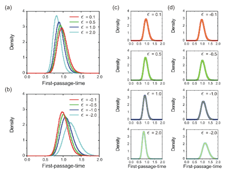
Figure 1: Comparison between the series solution for the FPT density function and numerical results. (a) and (b) First-passage-time distributions obtained from the numerical simulation of Eq. (1), for different (a) positive and (b) negative intensities of the time-dependent drift $\epsilon$ (colored histograms). (c) Each histogram shown in (a) is properly described by the series solution, Eq. (37), shown as a thin yellow line. (d) Equivalent comparison between theoretical results and the histograms shown in (b), for negative intensities. In each case, the series is truncated in an adequate order, $N$: $\phi(\tau)=\sum_{n=0}^{N}\epsilon^{n}~{}\phi_{n}(\tau)$. As the value of $\epsilon$ increases in magnitude, the order used to represent the theoretical result increases as well. In particular, $N=1$ for $\epsilon=\pm 0.1$ (top), $N=2$ for $\epsilon=\pm 0.5$ (middle-top), $N=4$ for $\epsilon=\pm 1.0$ (middle-bottom), and $N=9$ for $\epsilon=\pm 2.0$ (bottom). Parameters: $\mu=1$, $x_{\rm thr}-x_{0}=1$, $D=0.01$, and $\tau_{\rm d}=10$.

To illustrate the solution we have obtained for the FPT problem of a Brownian particle driven by an exponential time-dependent drift, in this section we compare the analytical results with data extracted from numerical simulations. Samples of the FPT distribution are collected from the times at which a Brownian particle, evolving according to the Langevin equation given by Eq. (1) and starting from $x_{0}$, arrives at the threshold $x_{\rm thr}$ for the first time. As we have shown in [31], for small intensities of the time-dependent drift, $\epsilon$, the system corresponds to a perturbation scenario, and the first-order solution, $\phi(\tau)=\phi_{0}(\tau)+\epsilon~{}\phi_{1}(\tau)$, properly describes the FPT statistics. In this section, we extend that comparison beyond the linear regime, for large values of $\epsilon$. Obviously, in this case we need to include higher order terms in the series given by Eq. (37). This comparison is not merely illustrative; since the characterization of the series convergence remains elusive to us, we resort to a numerical test case to demonstrate the usefulness of the series solution.
Considering $\epsilon=0$, the dynamics defined by Eq. (1) has no intrinsic timescale and, therefore, time units can be normalized by $(x_{\rm thr}-x_{0})/\mu$ (i.e. the external parameter $\mu$ defines the escape rate). Additionally, we consider the non-dimensional form of this equation, obtained by setting $x/(x_{\rm thr}-x_{0})\rightarrow x$, $\epsilon/(x_{\rm thr}-x_{0})\rightarrow\epsilon$, and $D/[(x_{\rm thr}-x_{0})\mu]\rightarrow D$. The preceding procedures are equivalent to set $\mu=1$ and $x_{\rm thr}-x_{0}=1$ in the system described by Eq. (1). Given our interest in neural adaptation, the remaining parameters will be defined from typical values in adapting neurons. For the system without the time-dependent drift, $\epsilon=0$, the mean FPT is $\langle\tau\rangle=1$; in the context we focus on, a proper scale for $\tau_{\rm d}$ is about $10$ times this value [16], $\tau_{\rm d}=10$. Since the squared noise intensity strongly influences the dispersion of the interspike interval distribution (FPT statistics), its value is selected to produce typical histograms obtained in experiments [6], $D=0.01$. The intensity of the time-dependent drift weights the influence of an adaptation current in the intrinsic FPT distribution (in particular, in the firing rate) and constitutes a negative feedback to the subthreshold integration [32] ($\epsilon<0$); given that our interest here is to analyse the behavior of the series solution, this parameter will be used to set different regimes beyond the linear case.
In Figs. (1.a) and (1.b) we show the FPT density function constructed from numerical data, for different intensities of the time-dependent exponential drift, $\epsilon$. As expected, for positive (negative) intensities, as the strength of the time-dependent drift increases in magnitude, the threshold is reached at earlier (later) times and, consequently, the FPT distribution shifts towards lower (larger) values. In Figs. (1.c) and (1.d), the different distributions are separately compared with analytical results. These results are based on the truncated series solution [see Eq. (37)], $\phi(\tau)=\sum_{n=0}^{N}\epsilon^{n}~{}\phi_{n}(\tau)$, where $N$ is selected to reproduce numerical data. As shown in Figs. (1.c) and (1.d) (top panel), the FPT distribution for $\epsilon=\pm 0.1$ is precisely described by the linear expansion (perturbation regime), $\phi(\tau)=\phi_{0}(\tau)\pm\epsilon~{}\phi_{1}(\tau)$. However, the proper description of the numerical distributions for higher intensities requires the addition of higher order terms. For example, as shown in Figs. (1.c) and (1.d), FPT distributions for $\epsilon=\pm 0.5$, $\epsilon=\pm 1.0$, and $\epsilon=\pm 2.0$ are described with $N=2$, $N=4$, and $N=9$, respectively (middle-top, middle-bottom, and bottom panels, respectively).
Except for the zeroth-order term, which can be explicitly computed in the temporal domain via the inverse Laplace transformation of Eq. (44) and known as the inverse Gaussian distribution [6],

$$\phi_{0}(\tau)=\frac{x_{\rm thr}-x_{0}}{\sqrt{4\pi D\tau^{3}}}~{}\exp\left\{-\frac{\left[(x_{\rm thr}-x_{0})-\mu\tau\right]^{2}}{4D\tau}\right\},$$ (46)

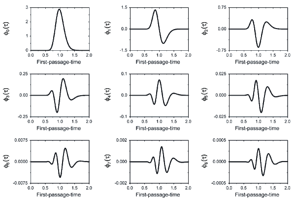
Figure 2: Functions $\phi_{n}(\tau)$ used to construct the theoretical description of the FPT statistics for the test case defined in Fig. (1). Note that the $y$-scale varies from panel to panel and, particularly, decreases as the order becomes higher.

all superior order functions, $\phi_{n}(\tau)$ for $n\geq 1$, require the numerical (inverse Laplace) transform of Eq. (2.4). In Fig. (2) we show these functions up to the eighth order, for the parameters defined in Fig. (1). It is worthwhile to note that these functions decrease in amplitude as the order increases (see $y$-scales), which is indicative of the convergence of the series (but not conclusive). An additional point to take into account in this analysis is that the numerical transform introduces an error which limits the reliability of the results. In particular, for the test case used here, the numerical inversion of the functions beyond the tenth order is inaccurate and, therefore, the comparison between analytical and numerical results is restricted to $\epsilon\sim\pm 2.0$ [Figs. (1.c) and (1.d)].
This numerical inaccuracy can be circumvented if we analyse properties that can be obtained directly from the Laplace transform of the FPT density function, $\tilde{\phi}^{L}(s)$; for example, its moments read [31]

$$\langle\tau^{k}\rangle=\int_{0}^{\infty}\phi(\tau)~{}\tau^{k}~{}{\rm d}\tau=(-1)^{k}~{}\frac{{\rm d}^{k}\tilde{\phi}^{L}(s)}{{\rm d}s^{k}}\Big{\rfloor}_{s=0}.$$ (47)

It is easy to check that, due to the linear nature, Eq. (47) adopts a series structure when $\tilde{\phi}^{L}(s)$ is replaced by Eq. (41). Explicitly, by defining

$$\langle\tau^{k}\rangle_{\phi_{n}}=(-1)^{k}~{}\frac{{\rm d}^{k}\tilde{\phi}_{n}^{L}(s)}{{\rm d}s^{k}}\Big{\rfloor}_{s=0},$$ (48)

Equation (47) results in

$$\langle\tau^{k}\rangle=\sum_{n=0}^{\infty}\epsilon^{n}~{}\langle\tau^{k}\rangle_{\phi_{n}}.$$ (49)

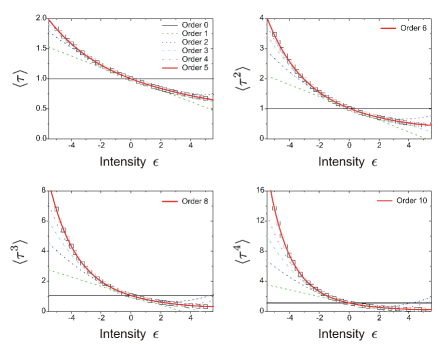
Figure 3: Comparison between numerical and theoretical results for the moments of the FPT distribution, as a function of the intensity of the time-dependent drift $\epsilon$. In all cases, symbols represent averages of numerical results, whereas lines correspond to Eq. (49) truncated at the order indicated. Parameters are defined as in Fig. (1).

In Fig. (3) we show a comparison between numerical and analytical results for the first four moments as a function of the intensity of the time-dependent drift. Parameters are defined as those corresponding to the test case analysed previously. This means that all $\langle\tau^{k}\rangle_{\phi_{n}}$ are certain scalars and Eq. (49) represents a polynomial in $\epsilon$. It is interesting to note that the order of the truncated polynomial, $N$, necessary to describe the numerical results increases as the exponent of the moment does. Alternatively, for a given order, the analytical expressions for the lowest moments remain valid in a larger range of $|\epsilon|$. Also, it is interesting to point out that Eq. (49) implies a different behavior for positive or negative values of $\epsilon$. As shown in Fig. (3), for $\epsilon<0$ the convergence of the analytical expression is smooth as the order of the polynomial increases, whereas for $\epsilon>0$ the convergence exhibits an alternating character.
From the moments of the FPT density function we can obtain other properties; in particular, its cumulants. In this case, the expressions relating both properties should be developed, and a series is obtained by grouping together equal order terms. For example, the second cumulant is, up to the first order in $\epsilon$, $\langle(\tau-\langle\tau\rangle)^{2}\rangle=\left[\langle\tau^{2}\rangle_{\phi_{0}}-\langle\tau\rangle^{2}_{\phi_{0}}\right]+\epsilon\left[\langle\tau^{2}\rangle_{\phi_{1}}-2\langle\tau\rangle_{\phi_{0}}\langle\tau\rangle_{\phi_{1}}\right]+\mathcal{O}(\epsilon^{2})$.

4 Concluding remarks and discussion

We have studied the FPT statistics resulting from the biased diffusion of a Brownian particle up to a threshold $x_{\rm thr}$, when the constant drift is supplemented with an exponential time-dependent component [see Eq. (1)]. In a previous work [31], we analysed this time-inhomogeneous system in the backward FP formalism, derived the diffusion equation governing the evolution of the survival probability from the backward state, Eq. (3), and proposed a solution as a series in terms of the intensity of the time-dependent drift, Eq. (6). In that work we focused on a perturbation regime and explicitly solved the expansion up to the first-order terms. In this work, we have extended these results by explicitly computing all superior order functions in a recursive scheme [see Eq. (2.2.2)]. The survival probability (with the initial state imposed) and the FPT statistics are easily derived from this solution and preserve the series structure; for completeness, their superior order terms are also explicitly given [see Eqs. (2.3.2) and (2.4), for the corresponding expressions in the Laplace domain]. In the second part of this work we have defined a test case in order to assess the usefulness of the series solution. Analytical and numerical results are compared for different intensities of the time-dependent drift (beyond the perturbation regime), and a remarkable agreement is found for each case whenever the series is truncated in an adequate order.
The problem we have analysed provides the intrinsic statistics of the events defined by an adapting neuron (interspike intervals). In this case, the system state corresponds to the membrane potential and the exponential time-dependent drift resembles a specific ionic current that decays during the subthreshold integration. This kind of currents supports a widely observed phenomenon in neurons, known as spike-frequency adaptation (SFA), when the initial state of the current (in the present framework, proportional to $\epsilon$) is properly coupled with the spiking history [32]. Particularly, they are restricted to be negative ($\epsilon<0$), providing a feedback to the neuron that lengths the interspike interval (FPT). In this work, we have focused on the statistics describing a single interspike interval for a given initial current [i.e. the FPT statistics analysed here corresponds to a conditional distribution, $\phi(\tau|\epsilon)$, in the history-dependent spike train]. As shown in [32], the analysis of the successive events in a neuron exhibiting SFA can be performed with a hidden Markov model. In this case, the conditional distribution is essential to study the spike train properties and its explicit assessment has motivated the contribution made in this study.

5 Acknowledgments

This work was supported by the Consejo de Investigaciones Científicas y Técnicas de la República Argentina.

References

Table 1: Coefficients $b_{n,k}(s)$ weighting the exponential terms that compose the solution to the survival probability and the FPT density function up to the fourth order. For the sake of clarity, we have defined the auxiliary coefficients $c_{n}(s)=[\mu-\sqrt{\mu^{2}+4D(s+n/\tau_{\rm d})}]/(2D)$.

Order	Coefficients
$n=1$	$b_{1,0}(s)=1$
	$b_{1,1}(s)=-1$
$n=2$	$b_{2,0}(s)=-[b_{1,0}(s)/2]c_{0}(s)=-\frac{1}{2}c_{0}(s)$
	$b_{2,1}(s)=-[b_{1,1}(s)/1]c_{1}(s)=c_{1}(s)$
	$b_{2,2}(s)=-b_{2,0}(s)-b_{2,1}(s)=\frac{1}{2}c_{0}(s)-c_{1}(s)$
$n=3$	$b_{3,0}(s)=-[b_{2,0}(s)/3]c_{0}(s)=\frac{1}{6}[c_{0}(s)]^{2}$
	$b_{3,1}(s)=-[b_{2,1}(s)/2]c_{1}(s)=-\frac{1}{2}[c_{1}(s)]^{2}$
	$b_{3,2}(s)=-[b_{2,2}(s)/1]c_{2}(s)=[-\frac{1}{2}c_{0}(s)+c_{1}(s)]c_{2}(s)$
	$b_{3,3}(s)=-b_{3,0}(s)-b_{3,1}(s)-b_{3,2}(s)=-\frac{1}{6}[c_{0}(s)]^{2}+\frac{1}{2}[c_{1}(s)]^{2}+[\frac{1}{2}c_{0}(s)-c_{1}(s)]c_{2}(s)$
$n=4$	$b_{4,0}(s)=-[b_{3,0}(s)/4]c_{0}(s)=-\frac{1}{24}[c_{0}(s)]^{3}$
	$b_{4,1}(s)=-[b_{3,1}(s)/3]c_{1}(s)=\frac{1}{6}[c_{1}(s)]^{3}$
	$b_{4,2}(s)=-[b_{3,2}(s)/2]c_{2}(s)=\frac{1}{2}[\frac{1}{2}c_{0}(s)-c_{1}(s)][c_{2}(s)]^{2}$
	$b_{4,3}(s)=-[b_{3,3}(s)/1]c_{3}(s)=\{\frac{1}{6}[c_{0}(s)]^{2}-\frac{1}{2}[c_{1}(s)]^{2}+[-\frac{1}{2}c_{0}(s)+c_{1}(s)]c_{2}(s)\}c_{3}(s)$
	$b_{4,4}(s)=-b_{4,0}(s)-b_{4,1}(s)-b_{4,2}(s)-b_{4,3}(s)$
	$\hskip 30.30225pt=\frac{1}{24}[c_{0}(s)]^{3}-\frac{1}{6}[c_{1}(s)]^{3}+\frac{1}{2}[-\frac{1}{2}c_{0}(s)+c_{1}(s)][c_{2}(s)]^{2}$
	$\hskip 42.67912pt+\{-\frac{1}{6}[c_{0}(s)]^{2}+\frac{1}{2}[c_{1}(s)]^{2}+[\frac{1}{2}c_{0}(s)-c_{1}(s)]c_{2}(s)\}c_{3}(s)$

References

- [1] van Kampen N G 2007 Stochastic Processes in Physics and Chemistry 3rd ed. (Amsterdam: North-Holland)
- [2] Ricciardi L M 1977 Diffusion Processes and Related Topics in Biology (Berlin: Springer-Verlag)
- [3] Hänggi P and Marchesoni F 2005 Chaos 15 026101
- [4] Redner S 2001 A Guide to First-Passage Processes (Cambridge: Cambridge University Press)
- [5] Tuckwell H C 1988 Introduction to Theoretical Neurobiology (Cambridge: Cambridge University Press)
- [6] Gerstein G L and Mandelbrot B 1964 Biophys. J. 4 41
- [7] Risken H 1989 The Fokker-Planck Equation: Methods of Solutions and Applications 2nd ed. (Berlin: Springer-Verlag)
- [8] Gardiner C W 1985 Handbook of Stochastic Methods: for physics, chemistry and the natural sciences 2nd ed. (Berlin: Springer-Verlag)
- [9] Lindner B and Longtin A 2005 J. Theor. Biol. 232 505
- [10] Tuckwell H C and Wan F Y M 1984 J. Appl. Prob. 21 695
- [11] Molini A, Talkner P, Katul G G and Porporato A 2011 Physica A 390 1841
- [12] Madison D V and Nicoll R A 1984 J. Physiol. 354 319
- [13] Helmchen F, Imoto K and Sakmann B 1996 Biophys. J. 70 1069
- [14] Sah P 1996 Trends Neurosci. 19(4) 150
- [15] Liu Y -H and Wang X -J 2001 J. Comput. Neurosci. 10 25
- [16] Benda J and Herz A V M 2003 Neural Comput. 15(11) 2523
- [17] Benda J, Maler L and Longtin A 2010 J. Neurophysiol. 104(5) 2806
- [18] Gerstner W and Kistler W M 2001 Spiking Neuron Models: Single Neurons, Populations, Plasticity (Cambridge: Cambridge University Press)
- [19] Burkitt A N 2006 Biol. Cybern. 95 1
- [20] Schwalger T, Fisch K, Benda J and Lindner B 2010 PLoS Comp. Biol. 6(12) e1001026
- [21] Gammaitoni L, Hänggi P, Jung P and Marchesoni F 1998 Rev. Mod. Phys. 70(1) 223
- [22] Bulsara A R, Lowen S B and Rees C D 1994 Phys. Rev. E 49(6) 4989
- [23] Gitterman M and Weiss G H 1995 Phys. Rev. E 52(5) 5708
- [24] Bulsara A R, Lowen S B and Rees C D 1995 Phys. Rev. E 52(5) 5712
- [25] Bulsara A R, Elston T C, Doering C R, Lowen S B and Lindenberg K 1996 Phys. Rev. E 53(4) 3958
- [26] Schindler M, Talkner P and Hänggi P 2004 Phys. Rev. Lett. 93(4) 048102
- [27] Burkitt A N 2006 Biol. Cybern. 95 97
- [28] Choi M H and Fox R F 2002 Phys. Rev. E 66 031103
- [29] Urdapilleta E and Samengo I 2009 Phys. Rev. E 80 011915
- [30] Lindner B 2004 J. Stat. Phys. 117(3/4) 703
- [31] Urdapilleta E 2011 Phys. Rev. E 83 021102
- [32] Urdapilleta E 2011 Phys. Rev. E 84 041904