Enhancement of Blackbody Friction due to the Finite Lifetime of Atomic Levels

Abstract

The thermal friction force acting on an atom moving relative to a thermal photon bath is known to be proportional to an integral over the imaginary part of the frequency-dependent atomic (dipole) polarizability. Using a numerical approach, we find that blackbody friction on atoms either in dilute environments or in hot ovens is larger than previously thought by orders of magnitude. This enhancement is due to far off-resonant driving of transitions by low-frequency thermal radiation. At typical temperatures, the blackbody radiation maximum lies far below the atomic transition wavelengths. Surprisingly, due to the finite lifetime of atomic levels, which gives rise to Lorentzian line profiles, far off-resonant excitation leads to the dominant contribution to the blackbody friction.

Introduction.—In Ref. MkPaPoSa2003 , the thermal drag force on an atom moving through a thermal bath at velocity $v$ has been calculated on the basis of the fluctuation-dissipation theorem. In a nutshell, the fluctuation-dissipation theorem states that any thermal fluctuation of a physical quantity (say, the electric field at finite temperature) is accompanied by corresponding fluctuations in the conjugate variable (here, the atomic dipole moment) provided the susceptibility (in the current case, the atomic polarizability) has a nonvanishing imaginary part. The imaginary part describes a dissipative process, in which the atom absorbs, then spontaneously emits, electromagnetic radiation. The dissipative fluctuations give rise to a drag force calculated using the Green–Kubo formula, as thoroughly explained in Ref. MkPaPoSa2003 . Further physical insight can be gained if one understands the process in terms of the direction-dependent Doppler effect MK1979bb . The atom absorbs blue-shifted blackbody photons coming in from the front, while emitting these photons in all directions, thereby losing kinetic energy due to net drain on its energy, and, as a consequence, on its momentum LaDKJe2011pra .

Here, we show that even more intriguing problems arise when one tries to evaluate the effect numerically, for simple atoms. In atomic physics, the width $\Gamma_{n}$ for each individual energy level $n$ needs to be determined separately. Atomic transitions can be driven even very far from resonance, albeit with small transition probabilities, The blackbody spectrum is distributed over the entire frequency interval $\omega\in[0,\infty)$, which leads to significant non-resonant contributions to the thermal friction.

The authors of Ref. MkPaPoSa2003 use correlation functions for the thermal electromagnetic fluctuations RyKrTa1989vol3 ; PiLi1958vol9 , in order to calculate the friction force acting on neutral, polarizable objects moving through uniform and isotropic thermal radiation. According to Eq. (12) of Ref. MkPaPoSa2003 , the effective friction (EF) force, which acts in a direction opposite to the velocity $v$, is given as a spectral integral,

$$F_{\rm EF}=-\frac{\beta\hbar^{2}\,v}{3\pi\,c^{5}\,(4\pi\epsilon_{0})}\int_{0}^{\infty}{\mathrm{d}}\omega\,\frac{\omega^{5}\,{\rm Im}\,\alpha(\omega)}{\sinh^{2}(\tfrac{1}{2}\beta\hbar\omega)}\,,$$ (1)

where $\beta=1/(k_{B}T)$ is the Boltzmann factor and $\alpha(\omega)$ is the dynamic polarizability of the atom. We here argue that the inclusion of the resonance widths due to the finite lifetimes of atomic levels is crucial in the calculation of the friction force. SI mksA units are used throughout this work.

Narrow and finite width.— If we assume that all atomic transitions are infinitely narrow (of width $\epsilon$), then

$$\alpha(\omega)=\sum_{n}\frac{f_{0n}}{2\omega_{0n}}\left(\frac{1}{\omega_{0n}-\omega-{\mathrm{i}}\epsilon}+\frac{1}{\omega_{0n}+\omega-{\mathrm{i}}\epsilon}\right)\,,$$ (2)

where $f_{0n}$ denotes the oscillator strength of the transition and $\omega_{0n}$ is the angular frequency for the transition from the ground state $|0\rangle$ to the excited state $|n\rangle$. In view of the Dirac prescription $1/(x-{\mathrm{i}}\epsilon)=P(1/x)+{\mathrm{i}}\pi\delta(x)$, the imaginary part of the polarizability is approximated as a sum of Dirac $\delta$ peaks,

$${\rm Im}\,\alpha(\omega)=\sum_{n}\frac{\pi f_{0n}}{2\omega_{0n}}\,\delta(\omega-\omega_{0n})\,.$$ (3)

However, if one includes the width $\Gamma_{n}$ of the excited states, then the starting expression (see Chap. 8 of Ref. Lo1993 ) for the dynamic polarizability reads

$$\alpha(\omega)= \;\sum_{n}\sum_{\pm}\frac{f_{0n}}{2\omega_{0n}}\;\frac{1}{\omega_{0n}-\frac{{\mathrm{i}}}{2}\Gamma_{n}(\omega)\pm\omega}\,,$$

$${\rm Im}\,\alpha(\omega)= \;\sum_{n}\frac{f_{0n}\,\Gamma_{n}(\omega)\;\omega_{0n}}{\big{(}\omega^{2}-\omega_{0n}^{2}\big{)}^{2}+\omega_{0n}^{2}\,\Gamma_{n}^{2}(\omega)}\,.$$ (4)

Here, the decay width $\Gamma_{n}(\omega)$ may be a function of the driving frequency $\omega$. In a number of places in the literature [e.g., see the text after Eq. (2) of Ref. LaSoPlSo2002 ], it is assumed that

$$\Gamma_{n}(\omega)=\overline{\Gamma}_{n}(\omega)=\frac{\omega}{\omega_{0n}}\Gamma_{n}\,,\qquad\Gamma_{n}\equiv\Gamma_{n}(\omega_{0n})\,.$$ (5)

One can justify the ansatz (5) in two ways (i) and(ii). (i) One may invoke an analogy with a damped, driven harmonic oscillator, whose Green function $g(t-t^{\prime})$ fulfills the defining differential equation

$$\left(-\frac{\partial^{2}}{\partial t^{2}}+\gamma\,\frac{\partial}{\partial t}+\omega_{0}^{2}\right)\overline{g}(t-t^{\prime})=\delta(t-t)\,,$$ (6)

so that the Fourier transform of the Green function reads as $\overline{g}(\omega)=1/(\omega_{0}^{2}-\omega^{2}-{\mathrm{i}}\,\gamma\,\omega)$, with

$${\rm Im}\;\overline{g}(\omega)=\frac{\gamma\,\omega}{\left(\omega^{2}-\omega_{0}^{2}\right)^{2}+\gamma^{2}\,\omega^{2}}\,.$$ (7)

Assuming that $\Gamma_{n}(\omega)=\overline{\Gamma}_{n}(\omega)$, this is proportional to the expression in (Enhancement of Blackbody Friction due to the Finite Lifetime of Atomic Levels) under the obvious identification $\omega_{0}\to\omega_{0n}$, $\gamma\to\Gamma_{n}$. (ii) The decay width $\Gamma_{n}$ enters the propagator denominators in Eq. (Enhancement of Blackbody Friction due to the Finite Lifetime of Atomic Levels) by a summation of self-energy insertions BeSa1957 . The imaginary of the self-energy, divided by $\hbar$, equals the decay width BaSu1978 . The velocity-gauge expression BeSa1957 ; Sa1994Mod ; Sa1967Adv for the decay rate, at resonance $\omega=\omega_{n}$ and off resonance (for general $\omega$), reads as

$$\Gamma_{n}= \;\frac{4\alpha}{3\pi}\,\omega_{0n}\,\frac{\left|\left<\Psi_{0}|\,\vec{p}\,|\Psi_{n}\right>\right|^{2}}{(mc)^{2}}\,,$$ (8a)

$$\overline{\Gamma}_{n}(\omega)= \;\frac{4\alpha}{3\pi}\,\omega\,\frac{\left|\left<\Psi_{0}|\,\vec{p}\,|\Psi_{n}\right>\right|^{2}}{(mc)^{2}}=\frac{\omega}{\omega_{0n}}\Gamma_{n}\,,$$ (8b)

where $\vec{p}$ is the momentum operator, and $\Psi_{0}$ and $\Psi_{n}$ are the wave functions of the ground and excited state.

By contrast, the so-called length gauge expression BeSa1957 ; Sa1994Mod ; Sa1967Adv for the decay width off resonance reads as

$$\Gamma_{n}= \;\frac{4\alpha}{3\pi}\,\omega_{0n}^{3}\,\frac{\left|\left<\Psi_{0}|\vec{x}|\Psi_{n}\right>\right|^{2}}{c^{2}}\,,$$ (9a)

$$\widetilde{\Gamma}_{n}(\omega)= \;\frac{4\alpha}{3\pi}\,\omega^{3}\,\frac{\left|\left<\Psi_{0}|\vec{x}|\Psi_{n}\right>\right|^{2}}{c^{2}}=\left(\frac{\omega}{\omega_{0n}}\right)^{3}\,\Gamma_{n}\,.$$ (9b)

For atoms, using the commutator relation $\vec{p}={\mathrm{i}}m[H,\vec{x}]/\hbar$, where $H$ is the Hamiltonian and $m$ the electron mass, one can show the equivalence of Eqs. (8a) and (9a) at resonance. The $\omega^{3}$ dependence off resonance in length gauge can be justified by analogy with Abraham–Lorentz radiative damping, with a damped oscillator Green function

$$\begin{split}\left(-\frac{\partial^{2}}{\partial t^{2}}-\frac{\gamma}{\omega_{0}^{2}}\,\frac{\partial^{3}}{\partial t^{3}}+\omega_{0}^{2}\right)\widetilde{g}(t-t^{\prime})=\delta(t-t)\,,\\ {\rm Im}\;\widetilde{g}(\omega)=\frac{\gamma\,\omega^{3}\,\omega_{0}^{2}}{\omega_{0}^{4}\,\left(\omega^{2}-\omega_{0}^{2}\right)^{2}+\gamma^{2}\,\omega^{6}}\,.\end{split}$$ (10)

Inserting the expression $\Gamma_{n}(\omega)=\widetilde{\Gamma}_{n}(\omega)$ into Eq. (Enhancement of Blackbody Friction due to the Finite Lifetime of Atomic Levels), one obtains the length-gauge form for the imaginary part of the polarizability off resonance ($\omega_{0}\to\omega_{0n}$, $\gamma\to\Gamma_{n}$).

Quite surprisingly, the question of whether one should use the length or velocity forms for the decay width off resonance, i.e., in the interval $0<\omega<\omega_{0n}$, has not been answered conclusively in the literature. It has often been stressed (e.g., in Ref. Ko1978prl ) that the electric field strength $\vec{E}$ is a physical observable and thus gauge invariant while the gauge-dependent vector potential $\vec{A}$ is not. Lamb noted in footnote 88 on p. 268 of Ref. La1952 that the interpretation of the quantum mechanical wave function is only preserved in the length gauge with the dipole $\vec{r}\cdot\vec{E}$ interaction, because the kinetic momentum changes from $\vec{p}\to\vec{p}-e\,\vec{A}$ in the presence of a vector potential, and therefore the $\vec{p}$ operator in the quantum mechanical Hamiltonian of the atom cannot be interpreted any more as a kinetic momentum if the vector potential is nonvanishing (see also Chap. XXI of Ref. Me1962vol2 and Refs. JeEvHaKe2003 ; EvJeKe2004 ). On the other hand, in Ref. LaSoPlSo2002 , the authors explain in the text after Eq. (2) that “the velocity [gauge] form follows originally from the [fully relativistic] QED description” and should therefore be used off resonance, for the obvious reason that the nonrelativistic limit of the Dirac matrix vector $\vec{\alpha}$, which enters the relativistic expression for the self-energy Mo1974a is the momentum operator $\vec{p}/(mc)$. While the length-gauge results seem to be generally preferred in the literature, the use of the length versus velocity forms remains controversial, and all numerical results below are therefore indicated for both velocity and length gauge; further considerations on the choice of the gauge are beyond the scope of the current article.

Figure 1: Plot of the integrand $x^{5}\,{\mathrm{e}}^{-b\,x}\,L_{s}(x)$ defined in Eq. (11b) in the interval characteristic of the thermal peak $x\approx 5/b=0.01583$ [Fig. (a), parameter $s=1$] and near the resonant peak $x\approx 0.375$ [Fig. (b), indistinguishable curves for $s=1$ and $s=3$]. The thermal peak [Fig. (a)] yields the dominant contribution to the model integral $J$ defined in Eq. (11a).

Model example.—In order to illustrate the numerical evaluation of Eq. (1), we consider a dimensionless model integral which is obtained by replacing frequency, transition width and $\beta$ with their dimensionless equivalents:

$$\omega \to x=\hbar\,\omega/E_{h},\hphantom{{}_{0}{}_{0}}\quad\Gamma\to\gamma=\hbar\,\Gamma/E_{h},\quad$$

$$\omega_{0} \to x_{0}=\hbar\,\omega_{0}/E_{h},\quad\beta\to b=\beta\,E_{h}=E_{h}/(k_{B}T),$$

where $E_{h}$ is the Hartree energy. The resulting integral

$$J= \;\int_{0}^{\infty}{\mathrm{d}}x\,x^{5}\,{\mathrm{e}}^{-b\,x}\,L_{s}(x)\,,$$ (11a)

$$L_{s}(x)= \;{\rm Im}\left[1/\left(x_{0}-x-\tfrac{{\mathrm{i}}\gamma}{2}\big{(}\tfrac{x}{x_{0}}\big{)}^{s}\right)\right]\,,$$ (11b)

contains the “Boltzmann factor” ${\mathrm{e}}^{-b\,x}$ which models the hyperbolic sine in the denominator of the integrand of Eq. (1), and the imaginary part is taken for a single resonance function that models the Lorentzian line profile [with $s=1$ and $s=3$ for the analogues of Eq. (8b) and Eq. (9b) respectively]. We choose the temperature as $T=1000\,K$, corresponding to $b=315.775$, and resonance parameters for the lowest (1S–2P) transition in the hydrogen atom: $x_{0}=\tfrac{3}{8}$, and $\gamma=1.5162\times 10^{-8}$. The imaginary part of the Lorentzian “polarizability term” $L_{s}(x)$ is highly peaked near the resonance energy $x=x_{0}$ and for $s=0$, and the full width at half maximum (FHWM) is equal to $\gamma$. The relative change of the prefactor $x^{5}\,\exp(-b\,x)$ over the interval $x\in(x_{0}-\tfrac{1}{2}\,\gamma,x_{0}+\tfrac{1}{2}\,\gamma)$ is smaller than $10^{-5}$. One thus conjectures that the replacement $L_{s}(x)\to\pi\,\delta(x-x_{0})$ should provide for an excellent numerical approximation to the contribution of the Lorentzian peak to the integral $J$. Indeed,

$$P_{1}= \;\int\limits_{0.374999}^{0.375001}\frac{{\mathrm{d}}x\,x^{5}}{{\mathrm{e}}^{b\,x}}\,L_{s}(x)=\left\{\begin{array}[]{l l}8.669\times 10^{-54}&\;\textrm{($s=1$)}\\ 8.669\times 10^{-54}&\;\textrm{($s=3$)}\\ \end{array}\right.\,,$$ (14)

$$P_{2}= \;\int\limits_{0.374999}^{0.375001}\frac{{\mathrm{d}}x\,x^{5}}{{\mathrm{e}}^{b\,x}}\,\pi\,\delta(x-x_{0})=8.711\times 10^{-54}\,,$$ (15)

confirming that $P_{1}\approx P_{2}$ for the peak term. However, this treatment ignores the possibility of far off-resonant driving of the transition for $x\ll x_{0}$. A numerical evaluation of the infrared thermal spectrum leads to the result

$$Q_{s}=\int\limits_{0}^{0.374999}\frac{{\mathrm{d}}x\,x^{5}}{{\mathrm{e}}^{b\,x}}\,L_{s}(x)=\left\{\begin{array}[]{l l}3.741\times 10^{-22}&\quad\textrm{($s=1$)}\\ 1.550\times 10^{-24}&\quad\textrm{($s=3$)}\\ \end{array}\right.,$$ (16)

which is larger than (14) by roughly 30 orders of magnitude. The exact numerical result for $J$ fulfills $J_{s}\approx Q_{s}$ to six decimals for $s=1$ and $s=3$; the effect is dominated by off-resonance absorption (see also Fig. 1).

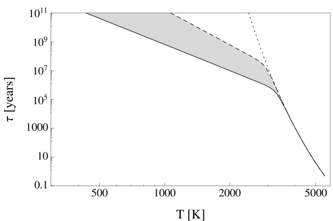
Figure 2: The characteristic slowdown time due to friction for ground state atomic hydrogen as a function of the blackbody radiation temperature. The solid line shows the results using the dynamic polarizability of Eq. (Enhancement of Blackbody Friction due to the Finite Lifetime of Atomic Levels) in length-gauge form [Eq. (9b)], the long-dashed line is the velocity-gauge form (8b), the shaded area is in between, and the short-dashed line results from Dirac $\delta$ peaks given in Eq. (3).

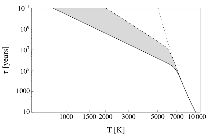
Figure 3: Same as Fig. 2 for a ground state helium atom.

Figure 4: Same as Figs. 2 and 3 for metastable helium ($2{{}^{3}}S_{1}$).

Table 1: Frequencies, oscillator strengths, lifetimes, and level widths for transitions between the ground $1$S state and $n^{1}$P levels within the hydrogen atom.

$n$	$\omega_{0n}$ [a.u.]	$f_{0n}$ [a.u.]	$1/\Gamma_{n}$ [ns]	$\Gamma_{n}$ [a.u.]
2	$0.375\,000\,000$	$0.416\,196\,717$	$1.595$	1.5162 10-8
3	$0.444\,444\,444$	$0.079\,101\,562$	$5.268$	4.5911 10-9
4	$0.468\,750\,000$	$0.028\,991\,029$	$12.346$	1.9507 10-9
5	$0.480\,000\,000$	$0.013\,938\,344$	$23.949$	1.0078 10-9

Table 2: Same as Table 1 for transitions between the ground $1^{1}$S state and the singlet $n^{1}$P levels within the helium atom.

$n$	$\omega_{0n}$ [a.u.]	$f_{0n}$ [a.u.]	$1/\Gamma_{n}$ [ns]	$\Gamma_{n}$ [a.u.]
2	$0.779\,881\,291$	$0.276\,1647$	$0.555$	4.3514 10-8
3	$0.848\,578\,015$	$0.073\,4349$	$1.728$	1.3998 10-8
4	$0.872\,654\,727$	$0.029\,8629$	$3.975$	6.0852 10-9
5	$0.883\,818\,387$	$0.015\,0393$	$7.653$	3.1607 10-9

Table 3: Same as Table 2 for transitions from the triplet metastable $2^{3}$S state to triplet $n^{3}$P levels (helium atom).

$n$	$\omega_{0n}$ [a.u.]	$f_{0n}$ [a.u.]	$1/\Gamma_{n}$ [ns]	$\Gamma_{n}$ [a.u.]
2	$0.042\,065\,187$	$0.539\,0861$	$98.202$	2.4623 10-10
3	$0.117\,148\,294$	$0.064\,4612$	$98.154$	2.4635 10-10
4	$0.142\,905\,024$	$0.025\,7689$	$142.886$	1.6923 10-10
5	$0.154\,678\,191$	$0.012\,4906$	$225.643$	1.0716 10-10

Simple Atoms.—Returning from our model example (11a) to realistic simple atoms, we provide results for the numerical integration of Eq. (1) for hydrogen atoms in Fig. 2 and for helium atoms in their ground and metastable triplet states in Figs. 3 and 4, respectively. The friction force is expressed in terms of its corresponding characteristic slowdown time $\tau=m\,v/F$. For atomic hydrogen and helium, the dynamic polarizability (Enhancement of Blackbody Friction due to the Finite Lifetime of Atomic Levels) has been used with the parameters listed in Tables 1—3. The input data have been partially calculated by us, and the transition frequencies and oscillator strengths have been verified against those given in Refs. Th1987 ; Dr2005 . The total decay rates used in the calculation include the decays to both ¹S and ¹D states. The temperature at which the full Lorentz profile results start to deviate from the Dirac-$\delta$ peaks is given by $T^{*}=\frac{\hbar\omega_{02}}{k_{B}x}$ where $x$ is the greater of the two real and positive (rather than complex) solutions of the equation $x^{7}{\mathrm{e}}^{-x}=\frac{32}{21}\pi^{5}\frac{\Gamma_{2}}{\omega_{02}}$ (velocity gauge) and $x^{9}{\mathrm{e}}^{-x}=\frac{128}{15}\pi^{7}\frac{\Gamma_{2}}{\omega_{02}}$ (length gauge, $n=2$ is the principal quantum number of the lowest excited state). For an equation of the form $x^{n}\,{\mathrm{e}}^{-x}=A$, this particular solution can be expressed as $x=-n\,W_{-1}(-A^{1/n}/n)$, where $W$ is the generalized Lambert $W$ function CoGoHaJeKn1996 . In velocity gauge, $T^{*}$ evaluates to $3293\,{\mathrm{K}}$ for hydrogen, $6927\,{\mathrm{K}}$ for singlet and $346{\mathrm{K}}$ for triplet helium. In length gauge we have $T^{*}=2954\,{\mathrm{K}}$ for hydrogen, $6208\,{\mathrm{K}}$ for singlet and $312\,{\mathrm{K}}$ for triplet helium (confirmed in Figs. 3 and 4).

Conclusions.—In this Letter, we show that far off-resonant driving of atomic transitions yields the dominant contribution to the blackbody friction force on moving atoms, due to the overlap of the infrared tail of the Lorentzian profile with the infrared thermal peak of the blackbody radiation. It is thus imperative to take the finite lifetime of the atomic resonances and their corresponding width into account. Numerical results for simple atoms are provided in Figs. 2—4. The feasibility of an experimental verification of the predictions of this Letter remains to be studied. Of the atomic systems considered here, the largest effect is expected for the metastable ³S₁ state in helium. In this case and for a temperature equal to the melting point of tungsten (3695K) the characteristic slowdown time is computed to be 3016s ($\approx 50$ minutes), which makes the friction effect difficult to observe in laboratory experiments, but perhaps not impossible. The general importance of an accurate understanding of blackbody friction for astrophysical processes has already been stressed in Ref. MkPaPoSa2003 . Further remarks on conceivable astrophysical consequences of the calculations reported here are beyond the scope of this Letter.

Acknowledgments.—This project was supported by NSF, DFG and a precision measurement grant (NIST).

References

- (1) V. Mkrtchian, V. A. Parsegian, R. Podgornik, and W. M. Saslow, Phys. Rev. Lett. 91, 220801 (2003).
- (2) J. M. McKinley, Am. J. Phys. 47, 602 (1979).
- (3) G. Łach, M. DeKieviet, and U. D. Jentschura, Einstein-Hopf drag, Doppler shift of thermal radiation and blackbody friction: A unifying perspective on an intriguing physical effect, submitted (2011).
- (4) S. M. Rytov, Y. A. Kravtsov, and V. I. Tatarskii, Principles of Statistical Radiophysics 3 (Springer, New York, 1989).
- (5) L. P. Pitaevskii and E. M. Lifshitz, Statistical Physics (Part 2) (Pergamon Press, Oxford, UK, 1958).
- (6) R. Loudon, The Quantum Theory of Light, 2 ed. (Clarendon Press, Oxford, 1993).
- (7) L. Labzowsky, D. Soloviev, G. Plunien, and G. Soff, Phys. Rev. A 65, 054502 (2002).
- (8) H. A. Bethe and E. E. Salpeter, Quantum Mechanics of One- and Two-Electron Atoms (Springer, Berlin, 1957).
- (9) R. Barbieri and J. Sucher, Nucl. Phys. B 134, 155 (1978).
- (10) J. J. Sakurai, Modern Quantum Mechanics (Addison-Wesley, Reading, MA, 1994).
- (11) J. J. Sakurai, Advanced Quantum Mechanics (Addison-Wesley, Reading, MA, 1967).
- (12) D. H. Kobe, Phys. Rev. Lett. 40, 538 (1978).
- (13) W. E. Lamb, Phys. Rev. 85, 259 (1952).
- (14) A. Messiah, Quantum Mechanics II (North-Holland, Amsterdam, 1962).
- (15) U. D. Jentschura, J. Evers, M. Haas, and C. H. Keitel, Phys. Rev. Lett. 91, 253601 (2003).
- (16) J. Evers, U. D. Jentschura, and C. H. Keitel, Phys. Rev. A 70, 062111 (2004).
- (17) P. J. Mohr, Ann. Phys. (N.Y.) 88, 26 (1974).
- (18) C. E. Theodosiou, At. Data Nucl. Data Tables 36, 97 (1987).
- (19) G. W. F. Drake, High Precision Calculations for Helium, Chap. 11 of the Handbook of Atomic, Molecular, and Optical Physics (Springer, New York, 2005).
- (20) R. M. Corless, G. H. Gonnet, D. E. G. Hare, D. J. Jeffrey, and D. E. Knut, Adv. Comput. Math. 5, 329 (1996).