On leave of absence from:]Department of Chemistry, School of Science,The University of Tokyo, 7-3-1 Hongo, Bunkyo-ku, Tokyo 113-0033, Japan

Triple Compton effect:
A photon splitting into three upon collision with a free electron

Abstract

The process in which a photon splits into three after the collision with a free electron (triple Compton effect) is the most basic process for the generation of a high-energy multi-particle entangled state composed out of elementary quanta. The cross section of the process is evaluated in two experimentally realizable situations, one employing gamma photons and stationary electrons, and the other using keV photons and GeV electrons of an x-ray free electron laser. For the first case, our calculation is in agreement with the only available measurement of the differential cross section for the process under study. Our estimates indicate that the process should be readily measurable also in the second case. We quantify the polarization entanglement in the final state by a recently proposed multi-particle entanglement measure.

Introduction.—The triple Compton effect is a fundamental process of light-matter interaction, in which a photon splits into three upon collision with an electron,

$${\textrm{e}}^{-}+\gamma\longrightarrow{\textrm{e}}^{-}+\gamma+\gamma+\gamma.$$ (1)

The cross section of this quantum electrodynamical (QED) process is of fourth order in the fine-structure constant $\alpha\approx 1/137.036$. Currently, there is no general theoretical treatment of the triple Compton effect in the literature. In principle, there is no limit of the number of photons that can be coherently emitted when an electron interacts with a photon, but the only processes which have been discussed so far are the usual, second-order (in $\alpha$) single Compton effect KlNi1929 and the third-order double Compton effect MaSk1952 . Only the single Compton effect has a classical limit. To the contrary, both the double and the triple Compton effects are intrinsically quantum processes which cannot be described by classical electrodynamics. With strong lasers becoming available, the nonlinear generalization of Compton scattering in which several laser photons are absorbed have been vigorously discussed; see HaHeIl2009 ; MaDPKe2010 for recent investigations of the nonlinear Compton effect, and LoJe2009prl ; LoJe2009pra ; SeKe2012 for a discussion on the nonlinear double Compton effect, where two photons are coherently emitted.

The three photons emitted in the process (1) originate from the same initial photon, are emitted at the same time, and are therefore quantum mechanically entangled. The creation of an entangled state of three photons is an important goal in quantum information. The conventional way of generating entangled triple-photon states is by employing nonlinear crystals PaEtAl2000 ; HuEtAl2000 ; AnGeKr2011 , but one can imagine other sources, not yet experimentally realized, such as electron-positron annihilation Gu1955 ; AbAdYo2011 . In this Letter, we propose the triple Compton effect as an alternative source of entangled photon triplets, which by suitable optimization could be competitive both in terms of production rate and the degree of entanglement. Especially interesting is the possibility of creating correlated photons with high energy in the GeV range, via triple Compton backscattering on a relativistic electron beam. We will show that a advantageous setup for such an experiment is an x-ray free electron laser (XFEL), providing a high-flux, high-energy photon beam together with a GeV electron beam.

The only previous experimental study of the triple Compton effect that we are aware of is Ref. MGBr1968 , where the differential cross section was measured for a well-defined interval of the solid angle, as defined by the detectors which were arranged in a symmetric angular configuration. On the theoretical side, the only preceding investigation is MaMaDh1959 , where the total cross section in the limit of ultra-relativistic initial photon energy was studied. In our treatment of the problem, we can evaluate the differential cross section for arbitrary values of the directions, energies and polarizations of the emitted photons. On the other hand, the double Compton effect is rather well studied, both experimentally MGBrKn1966 ; SaEtAl2000 ; SaSiSa2008 ; SaSiSa2011 and theoretically MaSk1952 ; RaWa1971 ; Go1984 . In addition, several other processes have been studied where two photons are produced in the final state, such as double bremsstrahlung BaEtAl1981 ; KrMaMaSt2002 ; KoSo2006 , bound state decay RaSuFr2008epjd ; JeSu2008 , and laser-induced photon splitting DPMiKe2007 , but comparatively little is known about triple photon production.

Theoretical formulation.—Unless stated otherwise, natural units with $\hbar=c=1$ are used, and $m$ denotes the electron mass. Four-vector products are denoted with a dot (i.e., we have $a\cdot b\equiv a^{\mu}\,b_{\mu}=a^{0}\,b^{0}-\bm{a}\cdot\bm{b}$ for two four-vectors $a$ and $b$). The contraction with the Dirac matrices $\gamma^{\mu}$ is written with a hat, $\hat{a}=a^{0}\gamma^{0}-\bm{a}\cdot\bm{\gamma}$.

We label the four-momenta of the incoming electron and photon with $p_{i}=(E_{i},\bm{p}_{i})$ and $k_{0}=\omega_{0}\,n_{0}=\omega_{0}\,(1,\bm{n}_{0})$, respectively, and the four-momenta of the outgoing electron and photons with $p_{f}=(E_{f},\bm{p}_{f})$, and $k_{j}=\omega_{j}n_{j}=\omega_{j}(1,\bm{n}_{j})$, $j=1,2,3$, respectively. When explicitly evaluating the cross section, we take the vectors $\bm{k}_{j}=\omega_{j}\bm{n}_{j}$ in the lab frame, in spherical coordinates with the polar axis directed along $\bm{k}_{0}$, i.e., $\bm{k}_{0}=\omega_{0}(0,0,1)$ and $\bm{k}_{j}=\omega_{j}(\sin\theta_{j}\cos\phi_{j},\sin\theta_{j}\sin\phi_{j},\cos\theta_{j})$. The amplitude $M$ for the triple Compton effect is formed from a coherent sum of $4!=24$ Feynman diagrams, one of which is shown in Fig. 1.

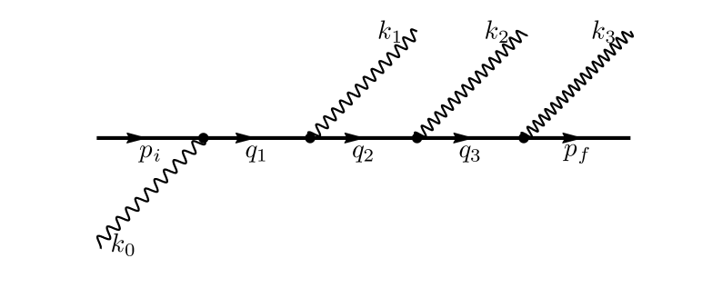
Figure 1: One of the $4!=24$ contributing Feynman diagrams of the triple Compton effect. To obtain the total amplitude, we have to add the diagrams corresponding to the permutations of the insertion order of the photons $k_{0}$, $k_{1}$, $k_{2}$, and $k_{3}$.

We have

$$M=m^{3}\sum_{\xi} u_{r_{f}}^{\dagger}(p_{f})\gamma^{0}\hat{\epsilon}_{\xi(3)}\frac{\hat{q}_{3}(\xi)+m}{q_{3}^{2}(\xi)-m^{2}}\hat{\epsilon}_{\xi(2)}\frac{\hat{q}_{2}(\xi)+m}{q_{2}^{2}(\xi)-m^{2}}$$

$$\times\hat{\epsilon}_{\xi(1)}\frac{\hat{q}_{1}^{2}(\xi)+m}{q_{1}^{2}(\xi)-m^{2}}\hat{\epsilon}_{\xi(0)}u_{r_{i}}(p_{i})\,,$$ (2)

where the sum runs over all the 24 permutations $\xi$ of $(0,1,2,3)$, and $r_{f}$ is the final electron spin. The momenta $q_{n}$ entering the propagators are defined as $q_{n}(\xi)=p_{i}+\sum_{j=0}^{n-1}(-1)^{\delta_{0\xi(j)}+1}\,k_{\xi(j)},$ where $\delta_{ij}$ is Kronecker’s delta function. (One adds to $p_{i}$ the four-momentum of the incoming photon $k_{0}$ and subtracts the four-momenta of the outgoing photons, according to the relevant permutation $\xi$.) In the expression for the amplitude (Triple Compton effect: A photon splitting into three upon collision with a free electron), we have introduced the positive-energy bispinor $u_{r}(p)$, with the spin index $r=1,2$, which we use in the conventions of Chap. 2 of ItZu1980 (the normalization is $\overline{u}_{r}(p)\,u_{r}(p)=u^{\dagger}_{r}(p)\,\gamma^{0}\,u_{r}(p)=1$). The polarization four-vectors $\epsilon_{j}=(0,\bm{\epsilon}_{j})$ satisfy $\epsilon_{j}\cdot k_{j}=0$ for $j=0,1,2,3$. As an explicit set of basis vectors for $\bm{\epsilon}_{j}$, we take $\bm{\epsilon}_{j}^{1}=(\cos\theta_{j}\cos\phi_{j},\cos\theta_{j}\sin\phi_{j},-\sin\theta_{j})$ and $\bm{\epsilon}_{j}^{2}=(-\sin\phi_{j},\cos\phi_{j},0)$. The differential cross section follows from the usual rules of QED JaRo1980 as

$$\frac{\mathrm{d}\sigma}{\mathrm{d}\omega_{1}\mathrm{d}\omega_{2}\mathrm{d}\Omega_{1}\mathrm{d}\Omega_{2}\mathrm{d}\Omega_{3}}\equiv\sigma_{5}={} \frac{\alpha^{4}}{(2\pi)^{4}}\frac{1}{m^{4}}\frac{\omega_{1}\,\omega_{2}\,\omega_{3}}{E_{f}\,p_{i}\cdot k_{0}}\frac{|M|^{2}}{|K|}$$

$$\times\Theta(\omega_{3})\Theta(E_{f}-m),$$ (3)

where $\Theta(\cdot)$ is the step function, $\mathrm{d}\Omega_{j}=\sin\theta_{j}\mathrm{d}\theta_{j}\mathrm{d}\phi_{j}$ is the differential solid angle of photon $j$, and we have introduced $\sigma_{5}$ as an abbreviation of the five-fold differential cross section. In Eq. (Triple Compton effect: A photon splitting into three upon collision with a free electron), the final four-momentum of the electron is fixed by energy-momentum conservation as $p_{f}=p_{i}+k_{0}-k_{1}-k_{2}-k_{3}$, and the energy of photon three is

$$\omega_{3}=\frac{p_{i}\cdot(k_{0}-k_{1}-k_{2})-k_{0}\cdot(k_{1}+k_{2})+k_{1}\cdot k_{2}}{n_{3}\cdot(p_{i}+k_{0}-k_{1}-k_{2})}.$$ (4)

The factor $K$ in (Triple Compton effect: A photon splitting into three upon collision with a free electron), arising from the final delta function integration over $\omega_{3}$ reads $K=1+\frac{\bm{n}_{3}\cdot(\bm{k}_{1}+\bm{k}_{2}-\bm{k}_{0}-\bm{p}_{i})+\omega_{3}}{E_{f}}$.

The differential cross section (Triple Compton effect: A photon splitting into three upon collision with a free electron) depends on eight continuous variables, two angles $\theta_{j}$, $\phi_{j}$ for each emitted photon and the energies $\omega_{1}$, $\omega_{2}$ of two of the emitted photons. The energy $\omega_{3}$ of the third photon is restricted by the kinematical constraints and is calculated by Eq. (4). In addition, we have six more discrete variables which can take any of two values, namely, the polarization vectors $\bm{\epsilon}_{j}$ of the photons and the spins $r_{i,f}$ of the electrons.

A couple of general remarks about the expression (Triple Compton effect: A photon splitting into three upon collision with a free electron) are the following. Similarly to the double Compton effect JaRo1980 , the cross section vanishes when all three photons are emitted parallel to the incoming photon. In the rest frame of the electron, this implies $\omega_{1}+\omega_{2}+\omega_{3}=\omega_{0}$ according to Eq. (4), and therefore corresponds to the incoming photon splitting into three photons without any interaction, which is not allowed. Whenever either of $\omega_{1}$, $\omega_{2}$ or $\omega_{3}$ goes to zero, $\sigma_{5}$ diverges as $1/\omega_{1,2,3}$, while the radiated energy remains finite in the infrared. This is the well-known infrared catastrophe of QED, which can be cured by adding radiative corrections BrFe1952 . In the current case, the divergences at $\omega_{n}\to 0$ would cancel against radiative corrections to the single and double Compton effect. The evaluation of such corrections is beyond the scope of this Letter. We will calculate the differential cross section sufficiently far from the infrared divergences, corresponding to a specific experimental detector threshold. Our calculations therefore have a relative accuracy of the order of the fine-structure constant.

Evaluation of the differential cross section.—The evaluation of $\sigma_{5}$ is performed numerically, by employing an explicit representation of $\gamma^{\mu}$ and $u_{r}(p)$. This approach is advantageous ScLoJeKe2007pra if one is interested in polarization-resolved cross sections, in which case the analytic evaluation of $\sigma_{5}$ does not simplify. We calculate the differential cross section (Triple Compton effect: A photon splitting into three upon collision with a free electron) for two different experimental setups. The first is the same as considered in Ref. MGBr1968 , were a measurement of the triple Compton cross section is described. In this setup, a gamma photon of energy $\omega_{0}=0.662$ MeV impinges on an electron at rest, $E_{i}=m$, and photons are detected in coincidence at $\theta_{1}=\theta_{2}=\theta_{3}=\pi/2$, and $\phi_{1}=2\pi/3$, $\phi_{2}=4\pi/3$, $\phi_{3}=0$. The photon energy threshold was $\omega_{n}\geq\varepsilon=13$ keV. What was actually measured was the differential cross section averaged over the solid angles subtended by the detectors,

$$\langle\sigma\rangle=\frac{1}{\Omega^{3}}\frac{1}{4}\sum_{\textrm{spin},\,\textrm{pol.}}\int_{\Omega}\mathrm{d}\Omega^{\prime}_{1}\mathrm{d}\Omega^{\prime}_{2}\mathrm{d}\Omega^{\prime}_{3}\int\mathrm{d}\omega_{1}\mathrm{d}\omega_{2}\sigma_{5},$$ (5)

where the solid angle is $\Omega=0.378$ sr, and the energy integration is over $\omega_{1,2,3}>\varepsilon$. Performing the integration in (5) over the angular intervals $\Delta\phi_{j}=\phi_{j}\pm\sqrt{\Omega}/2$, $\Delta\theta_{j}=\theta_{j}\pm\arcsin(\sqrt{\Omega}/2)$ so that $\int_{\Delta\theta_{j}}\mathrm{d}\cos\theta^{\prime}_{j}\int_{\Delta\phi_{j}}\mathrm{d}\phi^{\prime}_{j}=\Omega$, and over photon energies greater than $\varepsilon$, we obtain

$$\langle\sigma\rangle=4.1\times 10^{-9}\,{\rm b}/{\rm sr}^{3}\,.$$ (6)

This value should be compared to the measured value of

$$\langle\sigma\rangle^{\textrm{exp}}=(8.1\pm 2.4)\times 10^{-9}\,{\rm b}/{\rm sr}^{3}\,,$$ (7)

which includes an experimental uncertainty of 30% MGBr1968 . Although the calculated value lies outside the estimated experimental error bar (by $1.6$ standard deviations), we believe that our calculation rather can be regarded as a confirmation of the measurement in Ref. MGBr1968 , given the utmost difficult nature of the experiment. We have extended the analysis relevant to the experiment MGBr1968 to the energy interval $\omega_{0}\in(10^{-2},10^{2})$ MeV; details will be presented elsewhere.

The second example we consider is a triple Compton backscattering scheme: The head-on collision of a relativistic electron, at an incident energy of $E_{i}=5$ GeV and $\bm{p}_{i}=(0,0,-\sqrt{E_{i}^{2}-m^{2}})$, with an incoming photon of energy $\omega_{0}=1$ keV. Such parameters are realized in an XFEL, for example at the LCLS in Stanford LCLS , and would require the reflection of the x-ray beam to collide with the electron beam from the accelerator. In this situation, the photons are backscattered and emitted in a narrow cone around the propagation direction of the electron, $\theta_{j}\sim\pi-E_{i}/m$. We estimate the total cross section as $\sigma_{\rm TC}^{\textrm{tot}}=2\times 10^{-5}$ b, compared to $\sigma_{\rm DC}^{\textrm{tot}}=1\times 10^{-3}$ b and $\sigma_{\rm SC}^{\textrm{tot}}=3\times 10^{-2}$ b, where for DC and TC, we have assumed that all photons with energies larger than the assumed photon energy threshold $\varepsilon=50$ MeV are detected. If we adopt pulse parameters available at the LCLS LCLS , i.e., $2\times 10^{13}$ photons per pulse, $10^{9}$ electrons per bunch, a transverse bunch size of $40$ $\mu$m, perfect transverse overlap of the two pulses, and a repetition rate of 120 Hz, we obtain 3 triple photon events per second.

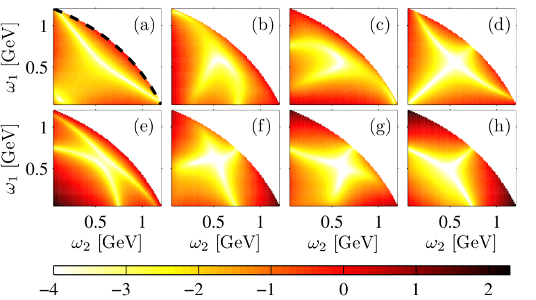
Figure 2: (color online). The five-fold differential cross section at $\theta_{j}=\pi-1.5\times 10^{-3}$ and $\phi_{j}=2j\pi/3$, $j=1,2,3$ as a function of $\omega_{1}$ and $\omega_{2}$. The color indicates the value of the cross section $\log_{10}(\frac{1}{2}\,\sum_{\textrm{spin}}\sigma_{5}/\textrm{b}\,\textrm{MeV}^{-2}\,\textrm{sr}^{-3})$ summed over the electron spins. We have $E_{i}=5$ GeV and $\omega_{0}=1$ keV, and the incoming photon beam is linearly polarized in the $x$-direction. The different panels correspond to different polarization of the final photons, we have $(\bm{\epsilon}_{1},\bm{\epsilon}_{2},\bm{\epsilon}_{3})=(\bm{\epsilon}_{1}^{j},\bm{\epsilon}_{2}^{k},\bm{\epsilon}_{3}^{l})$, with $jkl=$ (a) 111, (b) 211, (c) 121, (d) 112, (e) 221, (f) 212, (g) 122 and (h) 222. The black dashed line in panel (a) shows the curve along which the energy of photon three is at the assumed detector threshold, $\omega_{3}=\varepsilon=50$ MeV.

One example of the fully differential cross section in the XFEL setup is shown in Fig. 2. In this figure, we assume a configuration centered near the incoming electron axis, with $\theta_{j}=\pi-1.5\times 10^{-3}$ and $\phi_{j}=2j\pi/3$, $j=1,2,3$. We evaluate $\sigma_{5}$ as a function of $\omega_{1}$ and $\omega_{2}$. We sum over the electron spins, but assume a linearly polarized XFEL beam, and also fix the polarization of the emitted photons. We show $\sigma_{5}$ only for $\omega_{1,2,3}>\varepsilon$. For photon energies smaller than $\varepsilon$, the differential cross section is set to zero. It becomes clear from Fig. 2 that high energy photons in the GeV range can be achieved in this setup, which is interesting since it could provide correlated photon triplet states, with quantifiable entanglement as shown below, in an energy range which is far beyond what can be produced with down-conversion of photons in a nonlinear crystal PaEtAl2000 ; HuEtAl2000 ; AnGeKr2011 . The rate of 3 events/s obtained above is not small compared to the experimental results in HuEtAl2000 , where photon triplets produced from nonlinear down-conversion were detected at an event rate of 5 per hour. The polarization of GeV photons can be measured using coherent electron-positron pair production in aligned crystals ApEtAl2005 .

Entangled photon triplets.—The three photons in the final state are simultaneously emitted and their polarizations are inevitably entangled due to the quantum nature of the process. In general, the mixed polarization state resulting after the interaction can be described by the density matrix $\varrho$, which has matrix elements

$$\langle\lambda_{1}\lambda_{2}\lambda_{3}|\varrho|\lambda^{\prime}_{1}\lambda^{\prime}_{2}\lambda^{\prime}_{3}\rangle=N\sum_{r_{i},r_{f}}M(\lambda_{1}\lambda_{2}\lambda_{3})\,M^{\ast}(\lambda^{\prime}_{1}\lambda^{\prime}_{2}\lambda^{\prime}_{3}),$$ (8)

where we have written $M(\lambda_{1}\lambda_{2}\lambda_{3})=M(\bm{\epsilon}_{1}=\bm{\epsilon}_{1}^{\lambda_{1}},\bm{\epsilon}_{2}=\bm{\epsilon}_{2}^{\lambda_{2}},\bm{\epsilon}_{3}=\bm{\epsilon}_{3}^{\lambda_{3}})$, $\lambda_{j}\in\{1,2\}$, and the normalization constant $N$ is chosen so that $\operatorname{Tr}(\varrho)=1$ (we sum over initial and final electron spins $r_{i}$ and $r_{f}$). It is still an open problem and subject of active research how to quantify the entanglement of a given multi-particle state $\varrho$ (see Refs. ToGuSeUf2005 ; BaGiLiPi2011 ; JuMoGu2011 ). In the current study, we employ the entanglement measure put forward in JuMoGu2011 in order to estimate the degree of polarization entanglement present among the final three photons. Briefly, an entanglement witness $W$ is found by minimizing the trace $\operatorname{Tr}(W\varrho)$ with $W$ such that for all subsets $s$, $W=P_{s}+Q_{s}^{T_{s}}$, where $T_{s}$ denotes the partial transpose with respect to the subset $s$ LeKrCiHo2000 , and the matrices $P_{s}$, $Q_{s}$, $1-P_{s}$ and $1-Q_{s}$ should have positive eigenvalues. Then, $\tau(\varrho)=-\operatorname{Tr}(W\varrho)$ is a measure of the tripartite polarization entanglement present in $\varrho$. In particular, $\tau=0$ for states which are not genuinely tripartite entangled. As an example, $\tau(\varrho_{\textrm{GHZ}})=1/2$ for the Greenberger–Horne–Zeilinger (GHZ) state $\varrho_{\textrm{GHZ}}=|\textrm{GHZ}\rangle\langle\textrm{GHZ}|$, with $|\textrm{GHZ}\rangle=(|111\rangle+|222\rangle)/\sqrt{2}$ GrHoShZe1990 , so that $\tau=1/2$ may be regarded as maximum entanglement.

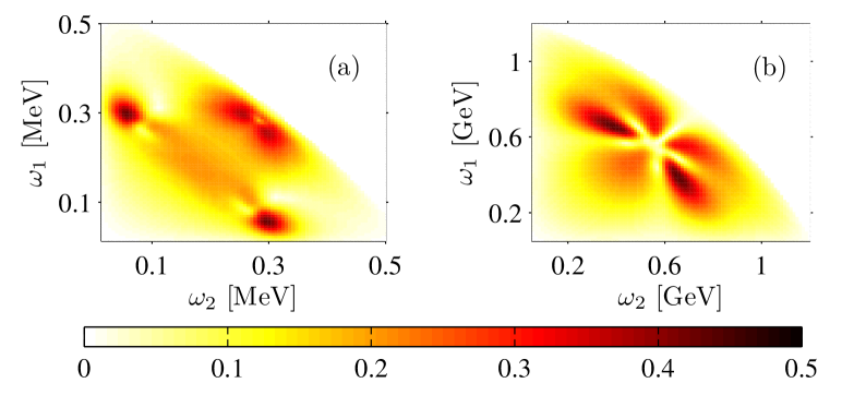
Figure 3: (color online). Entanglement measure $\tau$ as a function of the photon energies $\omega_{1}$ and $\omega_{2}$, for (a) $\omega_{0}=0.662$ MeV, $E_{i}=m$, $\theta_{j}=\pi/2-1$, $\phi_{j}=2j\pi/3$, $j=1,2,3$, $\varepsilon=13$ keV, and (b) $\omega_{0}=1$ keV, $E_{i}=5$ GeV, $\theta_{j}=\pi-1.5\times 10^{-3}$, $\phi_{j}=2j\pi/3$, $j=1,2,3$, $\varepsilon=50$ MeV. In both cases spin was summed over, and the initial photon beam was assumed to be linearly polarized in the $x$ direction. The differential cross section, and thus also $\tau$, was set to zero for photon energies below the detector threshold $\varepsilon$.

In Fig. 3, we show the value of $\tau$, evaluated as a function of $\omega_{1}$ and $\omega_{2}$ at (a) $\omega_{0}=0.662$ MeV, $E_{i}=m$, $\theta_{1,2,3}=\pi/2-1$, and $\phi_{j}=2j\pi/3$, and (b) $\omega_{0}=1$ keV, $E_{i}=5$ GeV, $\theta_{1,2,3}=\pi-1.5\times 10^{-3}$, and $\phi_{j}=2j\pi/3$ (the same situation as in Fig. 2). The numerical evaluation of $\tau$ was performed with pptmixer JuMoGu2011 , available at pptmixer . In both cases a non-zero value of $\tau$ for almost all values of $\omega_{1}$, $\omega_{2}$ where $\sigma_{5}>0$ shows that the three photons are indeed entangled. Almost maximum entanglement $\tau=1/2$ is achieved at certain places in the $\omega_{1}\omega_{2}$ plane.

Conclusions.—We have presented a theoretical study of the triple Compton effect, where a photon is split into three after colliding with an electron. Our formulation of the problem enables us to evaluate the differential cross section at arbitrary angles and energies of both initial and final particles. We verify the 44-year old experimental result reported in Ref. MGBr1968 . Theory and experiment are not in perfect agreement, but the discrepancy of roughly $1.6$ standard deviations is not significant [see Eqs. (6) and (7)]. Additional measurements are needed to clarify this issue. A straightforward generalization of the formalism to a Compton backscattering geometry then leads to theoretical predictions for the triple Compton effect for typical parameters at modern XFEL facilities, as shown in Fig. 2. Finally, while it is intuitively rather clear what a two-particle entangled quantum state is, the quantification of three-particle entanglement is a much more subtle problem. The entanglement measure $\tau$ has been proposed in Ref. JuMoGu2011 , and corresponding theoretical predictions in Fig. 3 show that the generation of a multi-particle entangled photon state in the MeV or GeV regime is possible based on the triple-Compton effect as a basic three-quanta emission process. The triplet photon final state is polarization entangled.

- (1) O. Klein and T. Nishina, Z. Phys. A 52, 853 (1929).
- (2) F. Mandl and T. H. R. Skyrme, Proc. Roy. Soc. London A 215, 497 (1952).
- (3) C. Harvey, T. Heinzl, and A. Ilderton, Phys. Rev. A 79, 063407 (2009).
- (4) F. Mackenroth, A. Di Piazza, and C. H. Keitel, Phys. Rev. Lett. 105, 063903 (2010).
- (5) E. Lötstedt and U. D. Jentschura, Phys. Rev. Lett. 103, 110404 (2009).
- (6) E. Lötstedt and U. D. Jentschura, Phys. Rev. A 80, 053419 (2009).
- (7) D. Seipt and B. Kämpfer, e-print arXiv:1201.4045 [hep-ph] (unpublished).
- (8) J.-W. Pan, D. Bouwmeester, M. Daniell, H. Weinfurter, and A. Zeilinger, Nature (London) 403, 515 (2000).
- (9) H. Hübel, D. R. Hamel, A. Fedrizzi, S. Ramelow, K. J. Resch, and T. Jennewein, Nature (London) 466, 601 (2010).
- (10) D. A. Antonosyan, T. V. Gevorgyan, and G. Y. Kryuchkyan, Phys. Rev. A 83, 043807 (2011).
- (11) S. N. Gupta, Phys. Rev. 99, 1015 (1955).
- (12) F. M. Abel, G. S. Adkins, and T. J. Yoder, Phys. Rev. A 83, 062502 (2011).
- (13) M. R. McGie and F. P. Brady, Phys. Rev. 167, 1186 (1968).
- (14) R. C. Majumdar, V. S. Mathur, and J. Dhar, Nuovo Cimento 12, 97 (1959).
- (15) M. R. McGie, F. P. Brady, and W. J. Knox, Phys. Rev. 152, 1190 (1966).
- (16) M. B. Saddi, R. Dewan, M. B. Saddi, and B. S. Ghumman, Nucl. Instrum. Meth. B 168, 329 (2000).
- (17) M. B. Saddi, B. Sing, and B. S. Sandhu, Nucl. Instrum. Meth. B 266, 3309 (2008).
- (18) M. B. Saddi, B. Sing, and B. S. Sandhu, Nucl. Tech. 175, 168 (2011).
- (19) M. Ram and P. Y. Wang, Phys. Rev. Lett. 26, 476 (1971), [Erratum Phys. Rev. Lett. 26, 1210 (1971)].
- (20) R. J. Gould, Astrophys. J. 285, 275 (1971).
- (21) V. N. Baier, V. S. Fadin, V. A. Khoze, and E. A. Kuraev, Phys. Rep. 78, 293 (1981).
- (22) A. A. Krylovetskiĭ, N. L. Manakov, S. I. Marmo, and A. F. Starace, Zh. Éksp. Teor. Fiz. 122, 1168 (2002), [JETP 95, 1006 (2002)].
- (23) A. V. Korol and I. A. Solovjev, Rad. Phys. Chem. 75, 1346 (2006).
- (24) T. Radtke, A. Surzhykov, and S. Fritzsche, Eur. Phys. J. D 49, 7 (2008).
- (25) U. D. Jentschura and A. Surzhykov, Phys. Rev. A 77, 042507 (2008).
- (26) A. Di Piazza, A. I. Milstein, and C. H. Keitel, Phys. Rev. A 76, 032103 (2007).
- (27) C. Itzykson and J. B. Zuber, Quantum Field Theory (McGraw-Hill, New York, 1980).
- (28) J. M. Jauch and F. Rohrlich, The Theory of Photons and Electrons, 2 ed. (Springer, Heidelberg, 1980).
- (29) L. M. Brown and R. P. Feynman, Phys. Rev. 85, 231 (1952).
- (30) S. Schnez, E. Lötstedt, U. D. Jentschura, and C. H. Keitel, Phys. Rev. A 75, 053412 (2007).
- (31) See the URL http://lcls.slac.stanford.edu.
- (32) A. Apyan, R. O. Avakian, B. Badelek, S. Ballestrero, C. Biino, I. Birol, P. Cenci, S. H. Connell, S. Eichblatt, T. Fonseca, A. Freund, B. Gorini, R. Groessa, K. Ispirian, T. J. Ketel, Y. V. Kononets, A. Lopez, A. Mangiarotti, B. van Rens, J. P. F. Sellschop, M. Shieha, P. Sona, V. Strakhovenko, E. Uggerhøj, U. I. Uggerhøj, G. Une, M. Velasco, Z. Z. Vilakaz, and O. Wessely, Nucl. Instrum. Meth. B 234, 128 (2005).
- (33) G. Tóth, O. Gühne, M. Seevinck, and J. Uffink, Phys. Rev. A 72, 014101 (2005).
- (34) J.-D. Bancal, N. Gisin, Y.-C. Liang, and S. Pironio, Phys. Rev. Lett. 106, 250404 (2011).
- (35) B. Jungnitsch, T. Moroder, and O. Gühne, Phys. Rev. Lett. 106, 190502 (2011).
- (36) M. Lewenstein, B. Kraus, J. I. Cirac, and P. Horodecki, Phys. Rev. A 62, 052310 (2000).
- (37) D. M. Greenberger, M. A. Horne, A. Shimony, and A. Zeilinger, Am. J. Phys. 58, 1131 (1990).
- (38) See the URL http://www.mathworks.com/matlabcentral/fileexchange/30968.