TeV Scale Phenomenology of $e^{+}e^{-}\to\mu^{+}\mu^{-}$ Scattering in the Noncommutative Standard Model with Hybrid Gauge Transformation

Abstract

The hybrid gauge transformation and its nontrivial phenomenological implications are investigated using the noncommutative gauge theory with the Seiberg-Witten map expanded scenario. Particularly, the $e^{+}e^{-}\to\mu^{+}\mu^{-}$ process is studied with a generalized noncommutative standard model (NCSM) including massive neutrinos and neutrino-photon interaction. In this model, the hybrid gauge transformation in the lepton sector is naturally introduced through the requirement of gauge invariance of the seesaw neutrino mass term. It is shown that in the NCSM without hybrid gauge transformation the noncommutative correction to the scattering amplitude of the $e^{+}e^{-}\to\mu^{+}\mu^{-}$ process appears only as a phase factor, predicting no new physical deviation in the cross section. However, when the hybrid feature is considered, the noncommutative effect appears in the single channel process. The cross section and angular distribution are analyzed in the laboratory frame including Earth’s rotation. It is proposed that pair production of muons in the upcoming TeV International Linear Collider (ILC) can provide an ideal opportunity for exploring not only the NC space-time, but also the mathematical structure of the corresponding gauge theory.

I Introduction

Although we are still far from a complete theory unifying quantum mechanics and general relativity, the noncommutative (NC) space-time is a common feature appearing in many existing theories of quantum gravity. The concept of noncommutative space-time was first introduced in Snyder’s pioneer work snyder1947 . Interest in noncommutative space-time has been revived in the recent decades due to its connection to string theory seiberg1999 ; Connes1998 (for a review, see Douglas2001 ). It is generally believed that the stringy effect can only be observed at the Planck scale $M_{P}$. However, given the scenario suggested by the extra-dimension theories extra that the large hierarchy between Planck scale $M_{P}$ and the weak scale $M_{W}$ can be strongly reduced, one can expect to see the NC effect at TeV scale, which is detectable in the LHC and other planned colliders. A popular noncommutative model is that the NC space-time is characterized by the coordinate operator satisfying

$$[\hat{x}_{\mu},\hat{x}_{\nu}]=i\theta_{\mu\nu}=\frac{ic_{\mu\nu}}{\Lambda^{2}_{NC}},$$ (1)

where the matrix matrix $\theta_{\mu\nu}$ is constant, antisymmetric and real, in units of $(\mathrm{mass})^{-2}$. The elements of the dimensionless constant matrix $c_{\mu\nu}$ are assumed to be of order unity, and $\Lambda_{NC}$ represents the NC scale. One can decompose the NC parameters $\theta_{\mu\nu}$ into two classes: electric-like component $\theta_{E}=(\theta_{01},\theta_{02},\theta_{03})$ associated with time-space noncommutativity and magnetic-like component $\theta_{B}=(\theta_{23},\theta_{31},\theta_{12})$ associated with space-space noncommutativity. Through the Weyl correspondence, the quantum field theory in NC space-time can be equivalent to that in commutative space-time with the ordinary product of field variables replaced by the Weyl-Moyal star product moyal

$$\phi_{1}*\phi_{2}(x)=\exp(\frac{i}{2}\theta^{\mu\nu}\partial_{\mu}^{x}\partial_{\nu}^{y})\phi_{1}(x)\phi_{2}(y)|_{y\rightarrow x}.$$ (2)

Using this method, the QED in noncommutative space-time (NCQED) has been constructed and extensively studied by many authors (for a review, see Szabo2003 ). However, to build a NC extension of the standard model (NCSM), one encounters some obstructions, such as charge quantization Haya and the no-go theorem Chaichian mms . Up to now, a minimal version of the noncommutative standard model (NCSM) has been proposed in Ref. Calmet1 , in which the consistency problem mentioned above is overcome when one generalizes the SU(3)*SU(2)*SU(1) Lie algebra gauge theory to the enveloping algebra value using the Seiberg-Witten map (SWM) method seiberg1999 . The SWM means that there is a map between the noncommutative fields and their classical counterparts as a power series expanded in $\theta$

$$\hat{\psi}(x,\theta) = \psi(x)+\theta\psi^{(1)}+\theta^{2}\psi^{(2)}+...$$ (3)

$$\hat{A}_{\mu}(x,\theta) = A_{\mu}(x)+\theta A^{(1)}_{\mu}+\theta^{2}A^{(2)}_{\mu}+...$$ (4)

where $\hat{\psi}$ and $\hat{A}_{\mu}$ denote the fields in NC space-time. The NCSM predicts not only NC correction of particle vertex but also new interactions beyond the standard model in ordinary space-time, e.g. $Z-\gamma-\gamma$ and $Z-g-g$ vertices behr03 . The rich phenomenological implications have led to intense studies of various high energy processes behr03 ; Das08 ; Sheng05 ; Pra2010 ; W2011 .

In the construction of NCSM, the so-called hybrid gauge transformation and hybrid SWM of Higgs fields are adopted to ensure covariant Yukawa terms Calmet1 . In this scenario, the Higgs fields feel a ”left” charge and a ”right” charge in NC gauge theory. Although only applied to the Higgs sector in Ref. Calmet1 , the method can in principle be extended to all other fields. One of the extensions has resulted in notable new physics predicted by NCQED: the tree-level interaction between neutrino and photon Sch04 . In NCQED, the interaction between fermion and photon are of three types: $e\hat{A}_{\mu}*\Psi$, $e\Psi*\hat{A}_{\mu}$ and $e(\hat{A}_{\mu}*\Psi-\Psi*\hat{A}_{\mu})$. The first two interaction are charge conjugated of each other. One can also consider it as the ambiguity in the ordering of Weyl-Moyal product. The third coupling is particularly interesting. In this case, the neutral particle transforms under NC U(1) gauge field from the left and right sides in a similar way as in the adjoint representation in the ordinary non-Abelian gauge theory. The covariant derivative is

$$\hat{D}_{\mu}\hat{\Psi}=\partial_{\mu}\hat{\Psi}-i[\hat{A_{\mu}},\hat{\Psi}]_{*}.$$ (5)

Then the action is invariant when $\Psi$ encounters the hybrid gauge transformation

$$\hat{\Psi}^{\prime}=U*\hat{\Psi}*U^{-1}$$ (6)

where $U=(e^{i\Lambda})_{*}$. The phenomenology of photon-neutrino interaction has been extensively explored Sch04 ; MME2006 . It is well known that one can not construct interactions such as $2e\hat{A}_{\mu}*\Psi-e\Psi*\hat{A}_{\mu}$ in the context of Lie algebra because the covariant derivatives can only be applied to the fermion fields of charged 0, $\pm 1$ Haya . However, as mentioned above, this restriction can be broken by extending the group structure from Lie algebra to the enveloping one with the help of SWM, as discussed in Sec. 2. We shall see below that this will lead to interesting phenomenological implication.

On the other hand, the NCSM in Ref. Calmet1 is constructed without including the neutrino mass. However, neutrino oscillation experiments have provided convincing evidence of massive neutrinos and lepton favor mixing neu2002 . Thus it is natural to question if the massive neutrinos and its direct interaction with photon as mentioned above can accommodate each other in the framework of NCSM. The issue has been studied in Ref. MM2008 . It is found that such an extension does not work for massive Dirac neutrino, while massive Majorana neutrinos are still consistent with the gauge symmetry. This means we have to accept the photon-neutrino interaction at the cost of ruling out the popular seesaw mechanisms neu1 ; neu2 that successfully generates Dirac neutrinos with small mass scale in the standard model and Majorana neutrinos with the GUT mass scale. In a recent work RH2011 , the authors showed that the difficulty presented in Ref. MM2008 can be overcome by appropriately generalizing the NC gauge transformation and SWM to a hybrid formation. In this sense, we can construct a generalized NCSM including the seesaw model and neutrino-photon interaction. The authors in Ref. RH2011 derived the Feynman rules of photon-neutrino interaction and Z boson-neutrino interaction in the NCSM incorporated with type I seesaw mechanism. As an phenomenological application, the $Z$ boson decays were studied in a very recent workZdecay .

It is interesting to investigate if generalization of the NCSM has any nontrivial effect on the phenomenology. A first choice is to explore the distinct neutrino-photon interaction which has been studied by many authors Sch04 ; MME2006 . In this paper, however, we focus our attention on a simple high energy process $e^{+}e^{-}\to\mu^{+}\mu^{-}$. The processes has been studied in Ref. Pra2010 using the NC corrected Feynman rules up to $\theta^{2}$ order. It has been shown that after considering all orders of the Seiberg-Witten map, the NC correction to the $e^{+}e^{-}\to\mu^{+}\mu^{-}$ appears only as phase factors, leaving no net noncommutative effect W2011 . In the generalized mNCSM, things are different. As we shall see later, the covariant derivatives of leptons require modifications to guarantee the gauge invariance of the Dirac-type mass term due to the presence of photon-neutrino interaction. We shall see that the modifications will have impact on the lowest order gauge coupling of charged leptons and eventually lead to a nontrivial NC correction for the scattering cross section. In Sec. 2, we first introduce the hybrid gauge transformation by considering the simplest case: the NCQED with $U(1)$ Abelian group. Then, we briefly review the NCSM incorporated with massive neutrino and neutrino-photon interaction given in Ref. RH2011 . The relevant Feynman rules involving all orders of the NC parameter $\theta$ are derived. In Sec. 3, we give the scattering amplitude of $e^{+}e^{-}\to\mu^{+}\mu^{-}$ in the laboratory frame where the earth rotational effect is considered. Numerical analyses of the total cross section and angular distribution are presented in Sec.4. We summarize our results in Sec.5.

II HYBRID GAUGE TRANSFORMATION IN NC GAUGE THEORIES

II.1 Hybrid Gauge Transformation in Noncommutative Abelian Theory

For simplicity, we start by investigating the Abelian NC $U(1)$ gauge theory. In this case, the NC Lagrangian for a fermion $\hat{\Psi}$ is

$$\hat{S}_{NC}=\int d^{4}x[i\bar{\hat{\Psi}}\gamma^{\mu}\hat{D}_{\mu}\hat{\Psi}-m\bar{\hat{\Psi}}\hat{\Psi}],$$ (7)

where $\hat{D}_{\mu}\hat{\Psi}=\partial_{\mu}\hat{\Psi}-ie\hat{A_{\mu}}*\hat{\Psi}$. The action is invariant under the gauge transformation

$$\hat{\Psi}^{\prime}(x,\theta)=U*\hat{\Psi}(x,\theta),$$ (8)

$$\hat{A}_{\mu}^{\prime}(x,\theta)=U*\hat{A}_{\mu}(x,\theta)*U^{-1}+\frac{i}{e}U*U^{-1},$$ (9)

where $U=(e^{i\Lambda})_{*}$. From the view point of gauge invariance, there is no priori requirement that we must take Eq.(8) as the only possible representation. In the enveloping algebra formulation, the NC gauge theory works well for arbitrary charges. With the help of SWM, one can extend Eq.(8) to the so-called hybrid formation in which the spinor $\hat{\Psi}$ proceeds under both ”left” and ”right” transformation:

$$\hat{\Psi}^{\prime}(x,\theta)=U_{L}*\hat{\Psi}(x,\theta)*U_{R}^{-1}$$ (10)

with $U_{L}=(e^{i\Lambda})_{*}$ and $U_{R}=(e^{i\Lambda^{\prime}})_{*}$. Then the corresponding covariant derivative is

$$\hat{D}_{\mu}\hat{\Psi}=\partial_{\mu}\hat{\Psi}-i(e+e^{\prime})\hat{A}_{\mu L}*\hat{\Psi}+ie^{\prime}\hat{\Psi}*\hat{A}_{\mu R},$$ (11)

where we define the ”left (right)” NC gauge fields $\hat{A}_{\mu L}$($\hat{A}_{\mu R}$) transforming as

$$\hat{A}_{\mu L}^{\prime}(x,\theta)=U_{L}*\hat{A}_{\mu L}(x,\theta)*U_{L}^{-1}+\frac{i}{e+e^{\prime}}U_{L}*U_{L}^{-1},$$ (12)

$$\hat{A}_{\mu R}^{\prime}(x,\theta)=U_{R}*\hat{A}_{\mu R}(x,\theta)*U_{R}^{-1}+\frac{i}{e^{\prime}}U_{R}*U_{R}^{-1}.$$ (13)

One can think of $\hat{\Psi}$ as having a ”left” charge $e+e^{\prime}$ and a ”right” charge $e^{\prime}$. However, $\hat{A}_{\mu L}$ and $\hat{A}_{\mu R}$ are gauge fields not for different particles but for the different NC representations of SWM of the ordinary gauge potential $A_{\mu}$. Up to the zeroth order of $\theta$, their expressions of SWM are the same: $\hat{A}_{\mu L}\simeq A_{\mu}\simeq\hat{A}_{\mu R}$. When the limit $\theta\rightarrow 0$ is taken, the NC covariant derivative Eq. (11) reduces to the ordinary one with the right electro-charge in commutative space-time. The hybrid feature presented here is derived from the degrees of freedom of NC gauge theory. The exact value of $e^{\prime}$ can not be constrained by the NC gauge invariance itself. In the existing literature, the $e^{\prime}$ is set to zero and the electron field $\hat{\Psi}$ only transforms as simplest representation Eq. (8). We believe that existence of more subtle representation is possible, and explore the phenomenological implication of it. The argument used in Abelian case can easily be extended to more realistic models. In the subsection B, we use a generalized NCSM as proposed in Ref. RH2011 , where the massive neutrinos and the photon-neutrino interaction is incorporated.

II.2 Hybrid Gauge Transformation in Noncommutative Standard Model

In this subsection, we briefly review the NCSM generalized by the seesaw mechanism and photon-neutrino interaction. Following the Ref. RH2011 , the action of the generalized NCSM is

$$\hat{S}_{GNCSM}=\hat{S}_{gauge}+\hat{S}_{quark}+\hat{S}_{lepton}+\hat{S}_{Higgs}+\hat{S}_{Yukawa},$$ (14)

where the gauge and quark sectors are the same as that in the NCSM of Ref. Calmet1 . However, we will see that the lepton, Higgs, and Yukawa sectors are modified to incorporate the seesaw mechanism and neutrino-photon interaction. In this paper, we only take the simplest type-I seesaw model into account, but the conclusion should be qualitatively applicable to other types. For our purpose, the Higgs and Yukawa sectors of the leptons are

$$\begin{split}\hat{S}_{Higgs}=&\int d^{4}x[(\hat{D}_{\mu}\hat{\Phi}_{d})^{\dagger}*(\hat{D}^{\mu}\hat{\Phi}_{d})-\mu^{2}\hat{\Phi}_{d}^{\dagger}*\hat{\Phi}_{d}-\lambda\hat{\Phi}_{d}^{\dagger}*\hat{\Phi}_{d}*\hat{\Phi}_{d}^{\dagger}*\Phi_{d}]\\ &+\int d^{4}x[(\hat{D}_{\mu}\hat{\Phi}_{s})^{\dagger}*(\hat{D}^{\mu}\hat{\Phi}_{s})-\mu^{2}\hat{\Phi}_{s}^{\dagger}*\hat{\Phi}_{s}-\lambda\hat{\Phi}_{s}^{\dagger}*\hat{\Phi}_{s}*\hat{\Phi}_{s}^{\dagger}*\Phi_{s}],\end{split}$$ (15)

$$\begin{split}\hat{S}_{Yukawa}&=\hat{S}_{Dirac}+\hat{S}_{Majorana}\\ &=-\int d^{4}x\sum_{i,j=1}^{3}[y_{ij}(\bar{\hat{\Psi}}_{L}^{i}*\hat{\Phi}_{d}*\hat{l}_{R}^{j})+y^{\dagger}_{ij}(\bar{\hat{l}}_{R}^{i}*{\hat{\Phi}}_{d}^{\dagger}*\hat{\Psi}_{L}^{j})\\ &+y^{\prime}_{ij}(\bar{\hat{\Psi}}_{L}^{i}*\hat{\Phi}_{d}^{c}*\hat{\nu}_{R}^{j})+y^{\prime\dagger}_{ij}(\bar{\hat{\nu}}_{R}^{i}*\hat{\Phi}_{d}^{c\dagger}*\hat{\Psi}_{L}^{j})]\\ &-\frac{i}{2}\int d^{4}x\sum_{i,j=1}^{3}[t_{ij}(\hat{\nu}_{R}^{iT}*\hat{\Phi}_{s}^{c}*\sigma_{2}\hat{\nu}^{j}_{R})-t_{ij}^{\dagger}(\hat{\nu}^{iT}_{R}*\hat{\Phi}_{s}^{c\dagger}*\sigma_{2}\hat{\nu}^{j}_{R})],\end{split}$$ (16)

where we have denoted the noncommutative left handed doublet of leptons, right handed singlet lepton, right handed neutrino, doublet Higgs boson and singlet Higgs fields respectively as

$$\hat{\Psi}_{L}=\begin{pmatrix}{\hat{\nu}_{L}}\\ {\hat{l}_{L}}\end{pmatrix},\quad\quad\hat{l}_{R},\quad\quad\hat{\nu}_{R},\quad\quad\hat{\Phi}_{d},\quad\quad\hat{\Phi}_{s},$$ (17)

respectively, and $i$, $j$ are the generation indices, and $y_{ij}$, $y^{\prime}_{ij}$ and $t_{ij}$ are Yukawa coupling constants. It is noted that in the generalized NCSM, we need not only the doublet Higgs fields but also a singlet Higgs fields to ensure the Majorana mass term of the right handed neutrino.

In ordinary space-time, the neutral-hyper-charged $\hat{\nu}_{R}$ singlet does not directly couple to any gauge field. However, in NC space-time, it can be coupled to the $U_{*}(1)$ hyper gauge field $\hat{B}_{\mu}$ through a star commutator

$$D_{\mu}\hat{\nu}_{R}=\partial_{\mu}\hat{\nu}_{R}-i\kappa g_{Y}[\hat{B}_{\mu},\hat{\nu}_{R}]_{*},$$ (18)

and $\hat{\nu}_{R}$ transforms under noncommutative $U_{*}(1)$ gauge group as

$$\delta_{\hat{\Lambda}}\hat{\nu}_{R}=i\kappa g_{Y}\hat{\Lambda}*\hat{\nu}_{R}-i\kappa g_{Y}\hat{\nu}_{R}*\hat{\Lambda},$$ (19)

where $\hat{\Lambda}$ is the gauge parameter and $\kappa$ is an unknown multiple or fractional number of the coupling constant. To ensure gauge invariance of the Yukawa sector Eq. (16), one can see that the transformation rules of the left-handed lepton doublet, right-handed charged lepton singlet, Higgs doublet, and Higgs singlet are respectively modified to

$$\begin{split}&\delta_{\hat{\Lambda}}\begin{pmatrix}{\hat{\nu}_{L}}\\ {\hat{l}_{L}}\end{pmatrix}=ig_{Y}[(-\frac{1}{2}+\kappa)\hat{\Lambda}*\begin{pmatrix}{\hat{\nu}_{L}}\\ {\hat{l}_{L}}\end{pmatrix}-\kappa\begin{pmatrix}{\hat{\nu}_{L}}\\ {\hat{l}_{L}}\end{pmatrix}*\hat{\Lambda}],\\ &\delta_{\hat{\Lambda}}\hat{l}_{R}=ig_{Y}[(-1+\kappa)\hat{\Lambda}*\hat{l}_{R}-\kappa\hat{l}_{R}*\hat{\Lambda}],\\ &\delta_{\hat{\Lambda}}\hat{\Phi}_{d}=ig_{Y}[(-\frac{1}{2}+\kappa)\hat{\Lambda}*\hat{\Phi}_{d}+(1-\kappa)\hat{\Phi}_{d}*\hat{\Lambda}],\\ &\delta_{\hat{\Lambda}}\hat{\Phi}_{s}=i\kappa g_{Y}\hat{\Lambda}*\hat{\Phi}_{s}-i\kappa g_{Y}\hat{\Phi}_{s}*\hat{\Lambda}.\end{split}$$ (20)

Compared with the configuration in Ref. Calmet1 , not only the Higgs fields but also the charged lepton fields show hybrid feature, where the fields transform under the gauge potentials from both the left and right sides. Thus, the covariant derivatives of the lepton fields are given by

$$D_{\mu L}\hat{\Psi}_{L}=\partial_{\mu}\hat{\Psi}_{L}-ig_{L}\hat{A}_{\mu}^{a}T^{a}*\hat{\Psi}_{L}-(-\frac{1}{2}+\kappa)g_{Y}\hat{B}_{\mu}*\hat{\Psi}_{L}+i\kappa g_{Y}\hat{\Psi}_{l}*\hat{B}_{\mu},$$ (21)

$$D_{\mu R}\hat{l}_{R}=\partial_{\mu}\hat{l}_{R}-i\kappa g_{Y}B_{\mu}*\hat{l}_{R}+i\kappa g_{Y}\hat{l}_{R}*B_{\mu},$$ (22)

where the $\hat{A}_{\mu}^{a}$ is the $SU(2)_{L}$ gauge potential and the $g_{L}$ is the coupling constant. Now we consider the lepton sector of the generalized mNCSM. Using Eqs. (21) and (22), the corresponding action is

$$\hat{S}_{lepton}=i\int d^{4}x[\bar{\hat{\Psi}}_{L}\gamma^{\mu}D_{\mu L}\hat{\Psi}_{L}+\bar{\hat{l}}_{R}\gamma^{\mu}D_{\mu R}\hat{l}_{R}].$$ (23)

The next step is to replace the NC fields in the action with their counterparts in ordinary space through appropriate Seiberg-Witten mapping. Usually, the SWM can be derived as perturbative solutions of the gauge equivalence relation order by order. Recently, the so-called $\theta$ exact Seiberg-Witten maps involving all orders of the NC parameter $\theta$ have been obtained by directly solving the gauge equivalence relation RH2011 ; exact2008 ; exact2011 or using the recursive formation of the Seiberg-Witten map W2011 . Here, we just list the results given in Ref. RH2011 :

$$\begin{split}&\hat{\Psi}_{L}=\Psi_{L}-\frac{\theta^{\mu\nu}}{2}(g_{L}A_{\mu}^{a}T^{a}-g_{Y}B_{\mu})\bullet\partial_{\nu}\Psi_{L}-\theta^{\mu\nu}\kappa g_{Y}B_{\mu}\star_{2}\partial_{\nu}\Psi_{L}+{\cal O}(a^{2})\Psi_{l},\\ &\hat{l}_{R}=l_{R}+\frac{\theta^{\mu\nu}}{2}g_{Y}B_{\mu}\bullet\partial_{\nu}l_{R}-\theta^{\mu\nu}\kappa g_{Y}B_{\mu}\star_{2}\partial_{\nu}l_{R}+{\cal O}(A^{2})l_{R},\\ &\hat{\nu}_{R}=\nu_{R}-\theta^{\mu\nu}\kappa g_{Y}B_{\mu}\star_{2}\partial_{\nu}\nu_{R}+{\cal O}(A^{2})\nu_{R},\\ &\hat{\Phi}_{d}=\Psi_{d}-\frac{\theta^{\mu\nu}}{2}(g_{L}A_{\mu}^{a}T^{a}+g_{Y}B_{\mu})\bullet\partial_{\nu}\Phi_{d}-\theta^{\mu\nu}(\kappa-1)g_{Y}B_{\mu}\star_{2}\partial_{\nu}\Phi_{d}+{\cal O}(A^{2})\Phi_{d,}\\ &\hat{\Phi}_{s}=\Psi_{s}-\theta^{\mu\nu}\kappa g_{Y}B_{\mu}\star_{2}\partial_{\nu}\Phi_{s}+{\cal O}(A^{2})\Phi_{s}\end{split}$$ (24)

with the extended products $\bullet$ and$\star_{2}$ defined by

$$f\bullet g:=f\begin{pmatrix}\frac{e^{\frac{i}{2}\theta^{\mu\nu}\overleftarrow{\partial}_{\mu}\overrightarrow{\partial}_{\nu}}-1}{\frac{i}{2}\theta^{\mu\nu}\overleftarrow{\partial}_{\mu}\overrightarrow{\partial}_{\nu}}\end{pmatrix}g,$$ (25)

$$f\star_{2}g:=f\begin{pmatrix}\frac{e^{\frac{i}{2}\theta^{\mu\nu}\overleftarrow{\partial}_{\mu}\overrightarrow{\partial}_{\nu}}-e^{-\frac{i}{2}\theta^{\mu\nu}\overleftarrow{\partial}_{\mu}\overrightarrow{\partial}_{\nu}}}{i\theta^{\mu\nu}\overleftarrow{\partial}_{\mu}\overrightarrow{\partial}_{\nu}}\end{pmatrix}g.$$ (26)

The notation ${\cal O}(A^{2})$ means we only consider the SWM to the first nontrivial order in the number of gauge potentials. Theoretically, it is difficult to obtain the analytic expressions of the higher order terms. We note, however, that for the processes $e^{+}e^{-}\to\mu^{+}\mu^{-}$, the number of gauge fields taking part in each vertex is not more than one. Thus, we can omit the higher order contribution. Substituting Eq. (24) into Eq. (23) and imposing spontaneous symmetry breaking under the unitary gauge, we can derive all the needed vertices. The corresponding Feynman rules are

$$-ie\gamma^{\mu}e^{\frac{i}{2}p_{1}\theta p_{2}}-2\kappa e\gamma^{\mu}\sin(\frac{1}{2}p_{1}\theta p_{2})$$ (27)

for the photon-electron-electron vertex, and

$$\frac{ie}{\sin 2\theta_{W}}\gamma^{\mu}(C_{V}-C_{A}\gamma^{5})e^{\frac{i}{2}p_{1}\theta p_{2}}+\frac{2\kappa e\sin\theta_{W}}{\cos\theta_{W}}\gamma^{\mu}\sin(\frac{1}{2}p_{1}\theta p_{2})$$ (28)

for the Z boson-electron-electron vertex. Here $p_{1}$ ($p_{2}$) is the momentum of the electron ingoing (outgoing) to the vertex; $p_{1}\theta p_{2}=p_{1}^{\mu}\theta_{\mu\nu}p_{2}^{\nu}$; $C_{V}=-\frac{1}{2}+2\sin^{2}\theta_{W}$, $C_{A}=-\frac{1}{2}$, and $\theta_{W}$ is the Weinberg angle. Since we are only concerned with the lowest tree-level process, the equations of motion are applied to the particles in the external lines and the terms vanish since the on-shell conditions are ignored. The vertex given above contains not only an exponent-type NC phase factor from the Moyal product W2011 but also a periodic term. The new NC term originates from massive neutrinos, photon-neutrino interaction, and requirement of gauge invariance. We shall see that this term leads to phenomenological implications in high energy processes.

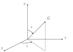
Figure 1: The primary coordinate system ($X-Y-Z$).

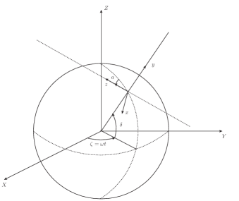
Figure 2: The laboratory coordinate system (x-y-z) on earth.

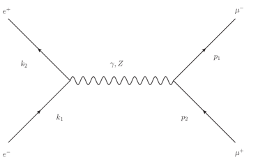
Figure 3: Feynman diagrams for process $e^{+}e^{-}\to\mu^{+}\mu^{-}$

III THE SCATTERING AMPLITUDE IN LABORATORY FRAME

In this section, we obtain the scattering amplitude of $e^{+}e^{-}\to\mu^{+}\mu^{-}$ in the laboratory frame. Although carrying the Lorentz index, the NC parameter $\theta_{\mu\nu}$ is assumed to be a fundamental constant, which does not change under the Lorentz transformation but does change with the observer frame. One can consider both the electric-like vector $\theta_{E}$ and the magnetic-like vector $\theta_{B}$ to be directionally fixed in a primary, un-rotational reference. Thus, the earth’s motion should be included when one discusses phenomenological processes in the lab frame. Let us define $(\hat{X},\hat{Y},\hat{Z})$ to be the orthonormal basis of this primary system (Fig. 1). In this frame the NC parameter vector can be written as

$$\theta_{E}=\frac{1}{{\Lambda_{E}^{2}}}(\sin{\eta_{E}}\cos{\xi_{E}}\hat{X}+\sin{\eta_{E}}\sin{\xi_{E}}\hat{Y}+\cos{\eta_{E}}\hat{Z}),$$ (29)

$$\theta_{B}=\frac{1}{{\Lambda_{B}^{2}}}(\sin{\eta_{B}}\cos{\xi_{B}}\hat{X}+\sin{\eta_{B}}\sin{\xi_{B}}\hat{Y}+\cos{\eta_{B}}\hat{Z}),$$ (30)

where $\eta$ and $\xi$ denote the NC polar angular and azimuth angular parameters with $0\leq\eta\leq\pi$ and $0\leq\xi\leq 2\pi$ respectively. However experiments are in laboratory frame $(\hat{x},\hat{y},\hat{z})$ on Earth (Fig. 2). We need a transformation matrix to correlate the two coordinate systems. Following the notations in Ref. Kam2007 , pkdas , we have

$$\left(\!\!\!\begin{array}[]{ccc}{\hat{X}}\\ {\hat{Y}}\\ {\hat{Z}}\end{array}\!\!\!\right)=\left(\!\!\!\begin{array}[]{ccc}c_{a}s_{\zeta}+s_{\delta}s_{a}c_{\zeta}&c_{\delta}c_{\zeta}&s_{a}s_{\zeta}-s_{\delta}c_{a}c_{\zeta}\\ -c_{a}s_{\zeta}+c_{\delta}s_{a}s_{\zeta}&{}_{\delta}s_{\zeta}&-s_{a}c_{\zeta}-s_{\delta}c_{a}s_{\zeta}\\ -c_{\delta}s_{a}&s_{\delta}&c_{\delta}c_{a}\end{array}\!\!\!\right)\left(\!\!\!\begin{array}[]{ccc}{\hat{x}}\\ {\hat{y}}\\ {\hat{z}}\end{array}\!\!\!\right),$$ (40)

where the abbreviation $c_{a}=\cos{a}$ etc. is used. The parameters $\delta$ and $a$ denote the location and orientation $-\frac{\pi}{2}\leq\delta\leq\frac{\pi}{2}$ and $0\leq a\leq 2\pi$ of the collider experiment. The parameter $\zeta$ is the rotation angle defined by $\zeta=\omega t$, where $\omega$ is the Earth’s angular velocity with $\omega=2\pi/{23h56m4.09s}$. Thus, the collider returns to its original position after a cycle of one day.

The tree-level Feynman diagram for $e^{+}e^{-}\to\mu^{+}\mu^{-}$ is shown in Fig. 3. The process is s-channel and proceed through photon and Z boson, like in the standard model. Using the Feynman rules in Sec. 2, the scattering amplitude is

$$\begin{split}M_{\gamma}=&-\frac{ie^{2}}{s}\bar{v}(k_{2})\gamma^{\mu}u(k_{1})\bar{u}(p_{1})\gamma_{\mu}v(p_{2})[ie^{\frac{i}{2}k_{2}\theta k_{1}}+2\kappa\sin(\frac{1}{2}k_{2}\theta k_{1})]\\ &\cdot[ie^{\frac{i}{2}p_{1}\theta p_{2}}+2\kappa\sin(\frac{1}{2}p_{1}\theta p_{2})]\end{split}$$ (41)

for $\gamma$ mediated interaction and

$$\begin{split}M_{Z}=&\frac{-ie^{2}}{s-m_{Z}^{2}+i\Gamma_{Z}}\bar{v}(k_{2})\gamma^{\mu}[\frac{i}{\sin{2\theta_{W}}}(C_{V}-C_{A}\gamma_{5})e^{\frac{i}{2}k_{2}\theta k_{1}}+2\kappa\tan_{\theta_{W}}\sin(\frac{1}{2}k_{2}\theta k_{1})]\\ &\cdot u(k_{1})\bar{u}(p_{1})\gamma^{\mu}[\frac{i}{\sin{2\theta_{W}}}(C_{V}-C_{A}\gamma_{5})e^{\frac{i}{2}p_{1}\theta p_{2}}+2\kappa\tan{\theta_{W}}\sin(\frac{1}{2}p_{1}\theta p_{2})]v(p_{2})\end{split}$$ (42)

for Z boson mediated interaction, where $k_{1}$, $k_{2}$, $p_{1}$ and $p_{2}$ are the four momenta of the ingoing electron, ingoing positron, outgoing muon, and outgoing anti-muon, respectively; $s=(k_{1}+k_{2})^{2}=(p_{1}+p_{2})^{2}$, and $\Gamma_{Z}$ is the decay width of the $Z$ boson. The total amplitude is

$$M=M_{\gamma}+M_{Z}.$$ (43)

In the center of mass reference,

$$\begin{split}&k_{1}=\begin{pmatrix}\frac{\sqrt{s}}{2},0,0,\frac{\sqrt{s}}{2}\end{pmatrix},\\ &k_{2}=\begin{pmatrix}\frac{\sqrt{s}}{2},0,0,-\frac{\sqrt{s}}{2}\end{pmatrix},\\ &p_{1}=\begin{pmatrix}\frac{\sqrt{s}}{2},\frac{\sqrt{s}}{2}\sin\theta\cos\phi,\frac{\sqrt{s}}{2}\sin\theta\sin\phi,\frac{\sqrt{s}}{2}\cos\theta\end{pmatrix},\\ &p_{2}=\begin{pmatrix}\frac{\sqrt{s}}{2},-\frac{\sqrt{s}}{2}\sin\theta\cos\phi,-\frac{\sqrt{s}}{2}\sin\theta\sin\phi,-\frac{\sqrt{s}}{2}\cos\theta\end{pmatrix},\\ \end{split}$$ (44)

where $\theta$ is the polar angle and $\phi$ is the azimuthal angle with respect to the initial beam direction along the z-axis. Using Eqs. (29), (30), (40) and (42), we obtain

$$\begin{split}&k_{2}\theta k_{1}=-\frac{s}{2\Lambda^{2}_{NC}}\Theta_{E}^{z},\\ &p_{2}\theta p_{1}=-\frac{s}{2\Lambda^{2}_{NC}}(\sin\theta\cos\phi\Theta_{E}^{x}+\sin\theta\sin\phi\Theta_{E}^{y}+\cos\theta\Theta_{E}^{z})\end{split}$$ (45)

with

$$\begin{split}&\Theta_{E}^{x}=s_{\eta}c_{\xi}(c_{a}s_{\zeta}+s_{\delta}s_{a}c_{\zeta})+s_{\eta}s_{\xi}(-c_{a}s_{\zeta}+c_{\delta}s_{a}s_{\zeta})-c_{\eta}c_{\delta}c_{a},\\ &\Theta_{E}^{y}=s_{\eta}c_{\xi}c_{\delta}c_{\zeta}+s_{\eta}s_{\xi}c_{\delta}c_{\zeta}+c_{\eta}c_{\delta},\\ &\Theta_{E}^{z}=s_{\eta}c_{\xi}(s_{a}s_{\zeta}-s_{\delta}c_{a}c_{\zeta})+s_{\eta}s_{\xi}(-s_{a}c_{\zeta}-s_{\delta}c_{a}s_{\zeta})+c_{\eta}c_{\delta}c_{a}.\end{split}$$ (46)

One can see that the process $e^{+}e^{-}\to\mu^{+}\mu^{-}$ is only sensitive to $\theta_{E}$. Then, the squared amplitude under spin-averaging is

$$\overline{|M|^{2}}=\overline{|M_{\gamma}|^{2}}+\overline{|M_{Z}|^{2}}+2\overline{Re(M_{\gamma}M^{\dagger}_{Z})}.$$ (47)

Using the tracing technique, the elements of squared amplitude are

$$\overline{|M_{\gamma}|^{2}}=\frac{e^{4}}{4s^{2}}[(k_{2}\cdot p_{1})(k_{1}\cdot p_{2})+(k_{2}\cdot p_{2})(k_{1}\cdot p_{1})]AB,$$ (48)

$$\overline{|M_{Z}|^{2}}=\frac{e^{4}}{4[(s-m_{Z}^{2})^{2}+\Gamma_{Z}^{2}m_{Z}^{2}]}[C_{+}(k_{2}\cdot p_{1})(k_{1}\cdot p_{2})+C_{-}(k_{2}\cdot p_{2})(k_{1}\cdot p_{1})],$$ (49)

$$2\overline{Re(M_{\gamma}M^{\dagger}_{Z})}=\frac{e^{4}(s-m_{Z}^{2})}{2s[(s-m_{Z}^{2})^{2}+\Gamma_{Z}^{2}m_{Z}^{2}]}[D_{+}(k_{2}\cdot p_{1})(k_{1}\cdot p_{2})+D_{-}(k_{2}\cdot p_{2})(k_{1}\cdot p_{1})],$$ (50)

where

$$A=32+128\kappa(\kappa-1)\sin^{2}(\frac{1}{2}k_{1}\theta k_{2}),$$ (51)

$$B=32+128\kappa(\kappa-1)\sin^{2}(\frac{1}{2}p_{2}\theta k_{1}),$$ (52)

$$\begin{split}C_{\pm}&=\frac{1}{\sin^{4}2\theta_{W}}\begin{bmatrix}32(C_{V}^{2}+C_{A}^{2})^{2}\pm 128C_{V}^{2}C_{A}^{2}\end{bmatrix}\\ &+\begin{bmatrix}-\frac{128\kappa C_{V}\tan\theta_{W}}{\sin^{3}2\theta_{W}}(C_{V}^{2}+C_{A}^{2}\pm 2C_{A}^{2})+\frac{128\kappa^{2}\tan^{2}\theta_{W}}{\sin^{2}2\theta_{W}}\end{bmatrix}\sin^{2}(\frac{1}{2}k_{1}\theta k_{2})\\ &+\begin{bmatrix}-\frac{128\kappa C_{V}\tan\theta_{W}}{\sin^{3}2\theta_{W}}(C_{V}^{2}+C_{A}^{2}\pm 2C_{A}^{2})+\frac{128\kappa^{2}\tan^{2}\theta_{W}}{\sin^{2}2\theta_{W}}(C_{V}^{2}+C_{A}^{2})\end{bmatrix}\sin^{2}(\frac{1}{2}p_{2}\theta p_{1})\\ &+\begin{bmatrix}\frac{512\kappa^{2}\tan^{2}\theta_{W}}{\sin^{2}2\theta_{W}}(C_{V}^{2}\pm C_{A}^{2})-\frac{1024\kappa^{3}C_{V}\tan^{3}\theta_{W}}{\sin 2\theta_{W}}+512\kappa^{4}\tan^{4}\theta_{W}\end{bmatrix}\sin^{2}(\frac{1}{2}k_{1}\theta k_{2})\\ &\cdot\sin^{2}(\frac{1}{2}p_{2}\theta p_{1}),\end{split}$$ (53)

$$\begin{split}D_{\pm}=&\frac{32}{\sin^{2}2\theta_{W}}(C_{V}^{2}\pm C_{A}^{2})+\begin{bmatrix}\frac{128\kappa(\kappa-0.5)C_{V}\tan\theta_{W}}{\sin 2\theta_{W}}-\frac{64\kappa(C_{V}^{2}\pm 2C_{A}^{2})}{\sin^{2}2\theta_{W}}\end{bmatrix}\sin^{2}(\frac{1}{2}k_{1}\theta k_{2})\\ &+\begin{bmatrix}\frac{128\kappa(\kappa-0.5)C_{V}\tan\theta_{W}}{\sin 2\theta_{W}}-\frac{64\kappa(C_{V}^{2}\pm 2C_{A}^{2})}{\sin^{2}2\theta_{W}}\end{bmatrix}\sin^{2}(\frac{1}{2}p_{2}\theta p_{1})\\ &+\begin{bmatrix}\frac{256\kappa^{2}C_{V}\tan\theta_{W}}{\sin 2\theta_{W}}-128\kappa^{2}\tan^{2}\theta_{W}\begin{pmatrix}1+\frac{C_{V}^{2}\pm C_{A}^{2}}{\sin^{2}2\theta_{W}}\end{pmatrix}\end{bmatrix}\cos(\frac{1}{2}k_{1}\theta k_{2})\cos(\frac{1}{2}p_{2}\theta p_{1})\\ &\sin(\frac{1}{2}k_{1}\theta k_{2})\sin(\frac{1}{2}p_{2}\theta p_{1})\\ &+\begin{bmatrix}\frac{256\kappa^{2}(1-2\kappa)C_{V}\tan\theta_{W}}{\sin 2\theta_{W}}+128\kappa^{2}\tan^{2}\theta_{W}\begin{pmatrix}1+\frac{C_{V}^{2}\pm C_{A}^{2}}{\sin^{2}2\theta_{W}}\end{pmatrix}+512\kappa^{3}(\kappa-1)\tan^{2}\theta_{W}\end{bmatrix}\\ &\sin^{2}(\frac{1}{2}k_{1}\theta k_{2})\sin^{2}(\frac{1}{2}p_{2}\theta p_{1}).\end{split}$$ (54)

In the calculation, the FeynCalc package of Mathematica COMPU is used and the fermion mass is neglected in the high energy limit.

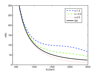
Figure 4: The total cross section $\langle\sigma\rangle_{T}$ after time averaging as a function of $E_{c}$ in ordinary space-time and noncommutative space-time for $\Lambda_{NC}=800$ GeV, $\eta=\frac{\pi}{4}$, and $\kappa=$1.3, -0.2, and 0.5.

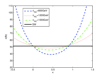
Figure 5: The total cross section $\langle\sigma\rangle_{T}$ after time averaging as a function of $\kappa$ for $E_{c}=1500$ GeV, $\eta=\frac{\pi}{4}$ rad, and $\Lambda_{NC}=800,1000,\mathrm{and}1200$ GeV.

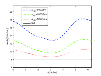
Figure 6: The time averaged $\langle\frac{d\sigma}{d\phi}\rangle_{T}$ as a function of $\phi$ for $E_{c}=1500$ GeV, $\kappa$=1.3, $\eta=\frac{\pi}{4}$ rad, and $\Lambda_{NC}=800,1000,\mathrm{and}1200$ GeV.

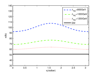
Figure 7: The time averaged $\langle\sigma\rangle_{T}$ as a function of $\eta$ for $E_{c}=1500$ GeV, $\kappa$=1.3, $\eta=\frac{\pi}{4}$ rad, and $\Lambda_{NC}=800,1000,\mathrm{and}1200$ GeV.

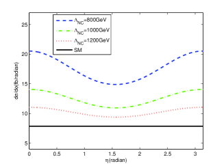
Figure 8: The time averaged $\langle\frac{d\sigma}{d\phi}\rangle_{T}$ as a function of $\eta$ for $E_{c}=1500$ GeV, $\kappa$=1.3, $\phi=5$ rad, and $\Lambda_{NC}=800,1000,\mathrm{and}1200$ GeV.

IV NUMERICAL ANALYSIS

In this section, we analyze the total cross section and angular distribution of the process $e^{+}e^{-}\to\mu^{+}\mu^{-}$ in the framework of the generalized NCSM. Because of the Earth’s rotation, it is difficult to get time-dependent data from the collider, so that the observable here should be averaged over a full day in order to compare them with the experimental results. The time-averaged differential cross section is

$$\langle\frac{d\sigma}{d\phi}\rangle_{T}=\frac{1}{T_{day}}\int_{0}^{T_{day}}\frac{d\sigma}{d\cos\theta d\phi}dt,$$ (55)

where the differential cross section for the two body process is given by

$$\frac{d\sigma}{d\cos\theta d\phi}=\frac{1}{64\pi^{2}s}\overline{|M|}^{2}.$$ (56)

After integrating, we get the timed-averaged total cross section

$$\langle\sigma\rangle_{T}=\frac{1}{T_{day}}\int_{0}^{T_{day}}dt\int_{-1}^{1}d(\cos\theta)\int_{0}^{2\pi}d\phi\frac{d\sigma}{d\cos\theta d\phi}.$$ (57)

IV.1 Time averaged total cross section and angular distribution

In Fig. 4, we show the ordinary total cross section $\sigma_{0}$ and the NC corrected total cross section $\langle\sigma\rangle_{T}$ as function of the collision energy $E_{c}(=\sqrt{s})$ for $\Lambda_{NC}=800$ GeV and $\kappa=1.3,0.5,\mathrm{and}-0.2$. The solid curve corresponds to the SM case. In our numerical analysis, we set the location coordinate of the laboratory frame at $(\delta,a)=(\frac{\pi}{4},\frac{\pi}{4})$, which is the location of the OPAL experiment at LEP. One can find from the figure that the NC effect causes significant deviation to the total cross section when $E_{c}$ is high enough. Interestingly, here $\langle\sigma\rangle_{T}$ is sensitive to both $\Lambda_{NC}$ and $\kappa$. When the NC scale parameter $\Lambda_{NC}$ is fixed, the total cross section can be enhanced or suppressed for different values of $\kappa$. To see more about this, we present $\langle\sigma\rangle_{T}$ as a function of the parameter $\kappa$ in Fig. 5 where $E_{c}(=\sqrt{s})$ is fixed at 1500 GeV, for $\Lambda_{NC}=800$ GeV, 1000 GeV and 1200 GeV. The horizontal line corresponds to the SM case. For simplicity, here we assume that $\kappa$ varies between -0.5 to 1.5. The figure shows that for a fixed collision energy the cross section has a parabolic dependence on $\kappa$. Despite different NC scale parameters at around 1 TeV, the total cross section is greatly enhanced when $\kappa$ is at [-0.5, 0] and about [0.9, 1.5]. If $\kappa$ is at about [0, 0.9], the cross section will be suppressed. We note that a similar picture also appears in Ref. W2011 , in which the deformation of covariant derivatives is due toa priori assumption and only limited to the Higgs sector. Thus, in that case no NC effect is manifested in the process $e^{+}e^{-}\to\mu^{+}\mu^{-}$. In Sec. 2, we have shown that the Feynman rules of electron-photon interaction and electron- Z boson interaction contain sin-type deformation coming from the consistency between the neutrino-photon interaction and seesaw extension of SM. As one of our main results, we show that this deformation indeed predicts interesting deviation from the total cross section.

We plot the the azimuthal angular distribution $\frac{d\sigma}{d\phi}$ in Fig.6 for $\Lambda_{NC}=800$ GeV, 1000 GeV and 1200 GeV. The horizontal line is for the SM case. Here the collision energy $E_{c}$ is $1500$ GeV and $\eta=\frac{\pi}{4}$. One can see from the figure that $\frac{d\sigma}{d\phi}$ is anisotropic. This is because the space-time noncommutativity is spontaneous Lorentz violation and breaking of rotational invariance. In our analysis, all three curves reach their maxima at around $\phi=5.58$ rad and their minima at $\phi=3.18$ rad. This unique feature can help us to identify the NC effect from the other effects.

IV.2 Time averaged total cross section and angular distribution as a function of $\eta$

Since $\theta_{E}$ is assumed to be a stationary vector fixed in the primary frame, any physical value calculated in NC space-time is not only sensitive to $\Lambda_{NC}$ but also to its direction parameter $(\eta,\xi)$. After taking the average over a full day rotation, $\eta$ remains. In Fig. 7, we present the $\langle\sigma\rangle_{T}$ and $\frac{d\sigma}{d\phi}$ as functions of $\eta$, for $E_{c}(=\sqrt{s})=$ 1500 GeV and $\kappa=$ 1.3. The curves show a positive kurtosis distribution for the whole range of $\eta$, and the horizonal solid line corresponds to the SM case. The maximum NC correction of all curves appear at $\eta=1.53$ rad. Thus, one can detect the NC effect for any $\theta_{E}$.

In Fig. 8, we plot $\langle\frac{d\sigma}{d\phi}\rangle_{T}$ as function of $\eta$ for $\Lambda_{NC}=800,1000,1200$ GeV. Here we fix the $\phi$ at 5 rad, $\kappa=1.3$ and collision energy $E_{c}=$ 1500 GeV. Different from $\langle\sigma\rangle_{T}$, the minima of the NC corrections are round $\phi=1.53$ rad.

V conclusion and discussion

In this work, we have considered a generalized noncommutative standard model, in which the massive neutrino and direct neutrino-photon interaction are included. It is found that the direct neutrino-photon interaction in NC space-time will have effect in the lepton sector and introduce hybrid gauge transformation by requiring gauge invariance. As an application, we study the TeV phenomenology of $e^{+}e^{-}\to\mu^{+}\mu^{-}$ scattering at $e^{+}e^{-}$ linear colliding. In NCSM without hybrid gauge transformation, it was found that when all orders of $\theta$ are included, there is no NC correction to the squared amplitude of $e^{+}e^{-}\to\mu^{+}\mu^{-}$ process. In the generalized NCSM, however, after deriving the corresponding Feynman rules, we find that there are additional sin-type deformations compared to the ones given in Ref. W2011 . These deformations lead to the nontrivial phenomenological implication that the cross section of $e^{+}e^{-}\to\mu^{+}\mu^{-}$ process can also have the NC effect, which is potentially detectable in the future International Linear Collider (ILC). The Earth’s rotation is also included. The cross section and angular distribution are analyzed in the laboratory frame. Pair production of muons via $e^{+}e^{-}$ collision in the ILC should provide an ideal opportunity for probing not only the NC space-time, but also the mathematical structure of the corresponding gauge theory.

Whether the deformed terms exist and how can one fix the value of $\kappa$ is still an open question. This may be because we still have not enough information on the renormalizability of the NC quantum field theory, where freedom of the deformation terms can be used to cancel the UV divergence Buric2002 . It is expected that further work on the renormalizability can remove these ambiguity. Before that one can treat it as an effective theory and the phenomenological study can give constraints on it, as has been done in the study of quarkonia decays Tamarit09 .

It is feasible to investigate other standard scatterings such as the Moller and Bhabha scattering. Although these processes are more kinematically complicated, they are ideal cases for detecting noncommutativity between space and space. This topic is interesting and deserve further study.

- (1) H. Snyder, Phys. Rev. 71, 38 (1947); H. Snyder, Phys. Rev. 72, 68 (1947).
- (2) A.Connes, M. R. Douglas, and A. Schwarz, J. High Energy Phys. 02, (1998) 003,
- (3) N. Seiberg, and E. Witten, J. High Energy Phys. 09, (1999) 032.
- (4) M. R. Douglas, and N. A. Nekrasov, Rev. Mod. Phys. 73, 977 (2001).
- (5) N. Arkani-Hamed, S. Dimopoulos and G. Dvali, Phys. Rev. D 59, 086004 (1999); L. Randall, and R. Sundrum, Phy. Rev. Lett. 83, 3370 (1999). E. Witten, Nucl. Phys. B 471, 135 (1996); P. Horava and E. Witten, Nucl. Phys. B 460, 506 (1996).
- (6) J. E. Moyal, Proc.Cambridge Phil. Soc. 45, 99 (1949).
- (7) R. J. Szabo, Phys. Rep. 378, 207 (2003).
- (8) M. Hayakawa, Phys. Lett. B 478, 394 (2000).
- (9) M. Chaichian, P. Presnajder, A. Tureanu, and M. M. Sheikh-Jabbari, Phys. Lett. B 526, 132 (2003).
- (10) X. Calmet, B. Jurco, P. Schupp, J. Wess, and M. Wohlgenannt, Eur. Phys. J. C 23, 363 (2002).
- (11) W. Behr, N. G. Deshpande, G. Duplancic, P. Schupp, J. Trampetic, and J. Wess, Eur. Phys. J. C 29, 441 (2003); M. Buric, D. Latas, V. Radovanovic and J. Trampetic, Phys. Rev. D 75, 097701 (2007).
- (12) B. Melic, K. Passek-Kumericki and J. Trampetic, Phys. Rev. D 72, 054004 (2005); A. Alboteanu, T. Ohl and R. Ruckl, Phys. Rev D 76, 105018 (2007); P. K. Das, N. G. Deshpande and G. Rajasekaran, Phys. Rev. D 77, 035010 (2008); S. K. Garg, T. Shreecharan, P. K. Das, N. G. Deshpande, G. Rajasekaran, J. High Energy Phys. 024, 1107 (2011).
- (13) Z. M. Sheng, Y. M. Fu, and H. Yu, Chin. Phys. Lett. 22, 561 (2005); Y. M. Fu and Z. M. Sheng, Phys. Rev. D75, 065025 (2007).
- (14) A. Prakash, A. Mitra and P. K. Das, Phys. Rev. D 82, 055020 (2010);
- (15) W. Wang, F. Tian, Z. M. Sheng, Phys. Rev. D 84, 045012 (2011);
- (16) P. Schupp, J. Trampetic, J. Wess, and G. Raffelt, Eur. Phys. J. C 36, 405 (2004); P. Minkowski, P. Schupp, and J. Trampetic, Eur. Phys. J. C 37, 123 (2004); R. Horvat, D. Kekez, P. Schupp, J. Trampetic, and J. You, Phys. Rev. D 84, 045004 (2011).
- (17) M. Haghighat, M. M. Ettefaghi, and M. Zeinali, Phys. Rev. D 73, 013007 (2006); R. Horvat, and J. Trampetic, Phys. Rev. D79, 087701 (2009); M. M. Ettefaghi, Phys. Rev. D 79, 065022 (2009); M. Haghighat, Phys. Rev. D 79, 025011 (2009); M. Zarei, E. Bavarsad, M. Haghighat, R. Mohammadi, I. Motie, and Z. Rezaei, Phys. Rev. D 81, 084035 (2010); R. Horvat, D. Kekez and J. Trampetic, Phys. Rev. D 83, 065013 (2011). M. M. Ettefaghi, T. Shakouri, J. High Energy Phys. 1011, (2010) 131; S. Bilmis et al., Phys. Rev. D 85, 073011 (2012).
- (18) SNO Collaboration, Q. R. Ahmad et al., Phys. Rev. Lett. 89, 011301 (2002); KamLAND Collaboration, K. Eguchi et al., Phys. Rev. Lett. 90, 021802 (2003); K2K Collaboration, M. H. Ahn et al., Phys. Rev. Lett. 90, 041801 (2003);
- (19) M. M. Ettefaghi, and M. Haghighat, Phys. Rev. D 77, 056009 (2008).
- (20) J.Schechter, J. W. F. Valle, Phys. Rev. D 22, 2227 (1980).
- (21) J.Schechter, J. W. F. Valle, Phys. Rev. D 25, 774 (1982).
- (22) R. Horvat, A, llakovac, P. Schupp, J. Trampetic, and J. You, arXiv: 1109.3085.
- (23) R. Horvat, A, llakovac, D. Kekez, J. Trampetic, and J. You, arXiv: 1204.6201.
- (24) P. Schupp, and Y. You, J. High Energy Phys. 08, (2008) 107;
- (25) R. Horvat, A, llakovac, P. Schupp, J. Trampetic, and J. You, arXiv: 1109.2485; R. Horvat, A, llakovac, P. Schupp, J. Trampetic, and J. You, arXiv: 1111.4951.
- (26) J. i. Kamoshita, Eur. Phys. J. C 52, 451(2007);
- (27) P. K. Das, and A, Prakash, arXiv: 1112.0943;
- (28) R. Mertig, M. Bohm, and A. Denner, Comput. Phys. Commun. 64, 345(1991);
- (29) M. Buric and V. Radovanovic, J. High Energy Phys. 10, (2002) 074; M. Buric, D. Latas and V. Radovanovic, J. High Energy Phys. 02, (2006) 046; D. Latas, V. Radovanovic and J. Trampetic, Phys. Rev. D76, 085006 (2007); M. Buric, V. Radovanovic and J. Trampetic, J. High Energy Phys. 03, (2007) 030; J. H. Huang and Z. M. Sheng, Phys. Lett. B 678, 250 (2009); M. Buric, D. Latas, V. Radovanovic and J. Trampetic, Phys. Rev. D77, 045031 (2008); M. Buric, D. Latas, V. Radovanovic and J. Trampetic, Phys. Rev. D 83, 045023 (2011);
- (30) C. Tamarit and J. Trampetic, Phys. Rev. D 79, 025020 (2009).