Informative priors and the analogy between quantum and classical heat engines

Abstract

When incomplete information about the control parameters is quantified as a prior distribution, a subtle connection emerges between quantum heat engines and their classical analogs. We study the quantum model where the uncertain parameters are the intrinsic energy scales and compare with the classical models where the intermediate temperature is the uncertain parameter. The prior distribution quantifying the incomplete information has the form $\pi(x)\propto 1/x$ in both the quantum and the classical models. The expected efficiency calculated in near-equilibrium limit approaches the value of one third of Carnot efficiency.

I Introduction

Quantum heat engines (QHEs) are novel tools to study the underlying thermodynamic properties of quantum systemsJohal2010 ; GRD2012 ; Scully ; Lutz ; ScullyPRL ; Noah2010 ; GRD2011 ; Kieu2004 . The working substance in a QHE is a few-level quantum system and can show interesting features like quantum correlation, coherence and so on. So QHEs may show unexpected behavior Scully ; Lutz ; ScullyPRL which is not possible in the classical models of heat engines. But all these models are consistent with the second law of thermodynamics. Recent studies Johal2010 ; GRD2012 showed that the expected behavior of certain models of QHE exhibit classical thermodynamic features which points out interesting and novel connection between information and thermodynamics. In these models, the uncertain parameters are treated as in Bayesian approach.

In Bayesian approach to probability theory, prior distribution Jeffreys1939 ; Jaynes1968 or known simply as a prior, quantifies the prior knowledge about the uncertain parameter(s). Usually, there is some information available even about the uncertain parameters, e.g. from the nature of the parameters or from the physics of the problem. The prior which makes use of this knowledge is also addessed as an informative prior. So the right choice of the prior plays an important role in this approach.

In this paper, we discuss a quantum and a classical model of heat engine and estimate their performance. In the quantum model we consider a pair of two level systems with energy level spacings $a_{1}$ and $a_{2}$. Reservoirs associated with the respective systems are at temperatures $T_{1}$ and $T_{2}$. These intrinsic energy level spacings can be controlled externally e.g. through external magnetic field. In the classical model, the pair of two level systems is replaced by a pair of classical ideal gas systems.

In the quantum model, the unknown parameters are the energy level spacings of the two level systems. But in the classical case, the uncertain parameter is the intermediate temperature. To assign the prior, we invoke different observers who satisfy a consistency criterion and thus arrive at the prior for the unknown parameter. These prior distributions are used to estimate the expected behavior of thermodynamic quantities. Finally we compare the estimated values of the physical quantities obtained from the quantum and the classical models. The main objective of this paper is to show the equivalence of the expected behavior of quantum and classical models under certain conditions. Interestingly the expected efficiencies are also related to the efficiencies at optimal performance for certain finite time models of Brownian heat engines.

The paper is organised as follows. In Section II, we present the quantum model for heat engine and summarise its main features. In Section III, we discuss the prior chosen in the quantum model based on the initial incomplete information about the internal energy scales of the working medium. In Section IV, we apply the prior so derived to estimate internal energies of the system. Further, we highlight a specific asymptotic limit in which the expected behavior becomes especially simple. Section V, we introduce the classical model with intermediate temperature as the uncertain parameter. The final Section VI is devoted to conclusions and future outlook.

II The Quantum model

Consider a pair of two-level systems labeled $R$ and $S$, with hamiltonians $H_{R}$ and $H_{S}$ having energy eigenvalues $(0,a_{1})$ and $(0,a_{2})$, respectively. The hamiltonian of the composite system is given by $H=H_{R}\otimes I+I\otimes H_{S}$. The initial state is $\rho_{\rm ini}=\rho_{R}\otimes\rho_{S}$, where $\rho_{R}$ and $\rho_{S}$ are thermal states corresponding to temperatures $T_{1}$ and $T_{2}$ ($<T_{1}$), respectively. Let ($r_{1},r_{2}$) and ($s_{1},s_{2}$) be the occupation probabilities of each system, where

$$r_{1}=\frac{1}{(1+e^{-a_{1}/T_{1}})},\qquad s_{1}=\frac{1}{(1+e^{-a_{2}/T_{2}})},$$ (1)

with $r_{2}=(1-r_{1})$ and $s_{2}=(1-s_{1})$. We have set Boltzmann’s constant $k_{\rm B}=1$. The initial mean energy of each system is

$$E_{\rm ini}^{(i)}=\frac{a_{i}}{(1+e^{a_{i}/T_{i}})},$$ (2)

where $i=1,2$ denote system $R$ and $S$ respectively. Based on quantum thermodynamics Gyftopoulos ; ABN2004 ; AJM2008 , the process of maximum work extraction is identified as a quantum unitary process on the thermally isolated composite system. It preserves not just the magnitude of Von Neumann entropy of the composite system, but also all eigenvalues of its density matrix. It has been shown in these works that for $a_{1}>a_{2}$, such a process minimises the final energy if the final state is given by $\rho_{\rm fin}=\rho_{S}\otimes\rho_{R}$. Effectively, it means that in the final state the two systems swap between themselves their initial probability distributions. The final energy of each system at the end of work extracting transformation is

$$E_{\rm fin}^{(i)}=\frac{a_{i}}{(1+e^{a_{j}/T_{j}})}.$$ (3)

where $i\neq j$. The average heat absorbed from system $R$ is defined as $Q_{1}={\rm Tr}[(\rho_{R}-\rho_{S})H_{R}]$, is given by

$$Q_{1}=a_{1}\left[\frac{1}{\left(1+e^{a_{1}/T_{1}}\right)}-\frac{1}{\left(1+e^{a_{2}/T_{2}}\right)}\right].$$ (4)

Similarly, the average heat released to system $S$ is defined as $Q_{2}={\rm Tr}[(\rho_{S}-\rho_{R})H_{S}]$, is given by

$$Q_{2}=-a_{2}\left[\frac{1}{\left(1+e^{a_{1}/T_{1}}\right)}-\frac{1}{\left(1+e^{a_{2}/T_{2}}\right)}\right].$$ (5)

The average work done in one cycle is $W=Q_{1}+Q_{2}$. To complete the cycle, the two systems are brought again in thermal contact with their respective reservoirs. The operation of the machine as a heat engine implies ${W}\geq 0$ and $Q_{1}\geq 0$, which is satisfied if

$$a_{1}(T_{2}/T_{1})\leq{a_{2}}\leq a_{1}.$$ (6)

III Prior Distribution

Now consider a situation in which the temperatures of the reservoirs are given a priori such that $T_{1}>T_{2}$, but the exact values of parameters $a_{1}$ and $a_{2}$ are uncertain. The prior information about these parameters may be summarised as follows:

• $a_{1}$ and $a_{2}$ represent the same physical quantity, i.e. the level spacing for system $R$ and $S$ respectively, and so they can only take positive real values.

• If the set-up of $R+S$ has to work as an engine, then criterion in Eq. (6) must hold, whereby if one parameter is specified, then the range of the other parameter is constrained.

Apart from the above conditions, we assume to have no information about $a_{1}$ and $a_{2}$. The question we address in the following is: What can we then infer about the expected behaviour of physical quantities for this heat engine ? We have suggested a subjective or Bayesian approach to address this question Johal2010 ; GRD2012 . This implies that an uncertain parameter is assigned a prior distribution, which quantifies our preliminary expectation about the parameter to take a certain value. Thus the prior should be assigned by taking into account any prior information we possess about the parameters. For example, if $a_{1}$ is specified, then the prior distribution for $a_{2}$, $\pi(a_{2}|a_{1})$ is conditioned on the specified value of $a_{1}$, and is defined in the range $[a_{1}\theta,a_{1}]$, where $\theta=T_{2}/T_{1}$, because we know the set-up works like an engine if we implement Eq. (6). We denote the prior distribution function for our problem by $\Pi(a_{1},a_{2})$. To assign the prior, it seems convenient to involve two observers $A$ and $B$, who wish to assign priors for $a_{1}$ and $a_{2}$. Based on the derivation given in GRD2012 , we find that the prior for each parameter is

$$\Pi(a_{i})=\frac{1}{\ln{\left(\frac{a_{\rm max}}{a_{\rm min}}\right)}}\frac{1}{a_{i}},$$ (7)

and the joint prior for the system acting as an engine, is given by

$$\Pi(a_{1},a_{2})=\frac{1}{\ln\left({\frac{1}{\theta}}\right)\ln{\left(\frac{a_{\rm max}}{a_{\rm min}}\right)}}\frac{1}{a_{1}a_{2}}.$$ (8)

IV Expected Values of Quantities

In this section, we use the priors assigned above, to find expected values for various physical quantities related to the engine. The expected value of any physical quantity $X$ which may be function of $a_{1}$ and $a_{2}$, is defined as follows:

$$\overline{X}=\int\int X\,\Pi(a_{1},a_{2})\,da_{1}da_{2}.$$ (9)

These expected values reflect the estimates by an observer who assigns the priors. In principle, there are two ways to calculate the expected value of some quantity which depends, in general, on the method used. The method by which the observer $A$ applies the joint prior is based on the definition

$$\Pi(a_{1},a_{2})=\Pi(a_{2}|a_{1})\Pi(a_{1}),$$ (10)

i.e. the prior for $a_{1}$ is assigned first, followed by $\Pi(a_{2}|a_{1})$ which is the conditional distribution of $a_{2}$ for a given value of $a_{1}$. On the other hand, observer $B$ applies

$$\Pi(a_{1},a_{2})=\Pi(a_{1}|a_{2})\Pi(a_{2}),$$ (11)

whereby the prior for $a_{2}$ is assigned first and $\Pi(a_{1}|a_{2})$ represents the conditional distribution of $a_{1}$ for a given value of $a_{2}$.

IV.1 Internal energy

We calculate the expected values of internal energies for systems $R$ and $S$. These values can then be used to find the expected work per cycle, heat exchanged and so on.

(i) Initial state: For a given $a_{i}$, the internal energy $E_{\rm ini}^{(i)}$ is given by Eq. (2). The expected initial energy is defined as

$$\overline{E}_{\rm ini}^{(i)}=\int_{a_{\rm min}}^{a_{\rm max}}E_{\rm ini}^{(i)}\Pi(a_{i})da_{i},$$ (12)

where $i=1,2$. Note that $E_{\rm ini}^{(i)}$ depends only on $a_{i}$, so we need to average over the prior for $a_{i}$ only. Using Eqs. (2) and (7), we obtain

$$\overline{E}_{\rm ini}^{(i)} = {\left[\ln{\left(\frac{a_{\rm max}}{a_{\rm min}}\right)}\right]}^{-1}$$

$$\times\left[(a_{\rm max}-a_{\rm min})+T_{i}\ln{\left(\frac{1+e^{a_{\rm min}/T_{i}}}{1+e^{a_{\rm max}/T_{i}}}\right)}\right].$$

(ii) Final state : In this case, the internal energy of $R$ as well as $S$, is function of both $a_{1}$ and $a_{2}$ (see (3)) and so the expected values are obtained by averaging over the joint prior, $\Pi(a_{1},a_{2})$. For instance, the expected final energy of system $S$ (denoted by superscript (2)) as calculated by $A$ is

$$\overline{E}_{\rm fin}^{(2)}({A}) = \int\int E_{\rm fin}^{(2)}\,\Pi(a_{2}|a_{1})\Pi(a_{1})\,da_{1}da_{2}$$

$$= K\int_{a_{\rm min}}^{a_{\rm max}}\frac{1}{(1+e^{a_{1}/T_{1}})a_{1}}da_{1}\int_{a_{1}\theta}^{a_{1}}da_{2},$$

$$= K\left(1-\theta\right)$$

$$\times\left[(a_{\rm max}-a_{\rm min})+T_{1}\ln{\left(\frac{1+e^{a_{\rm min}/T_{1}}}{1+e^{a_{\rm max}/T_{1}}}\right)}\right].$$

where $K=[\ln{(1/\theta)}\ln{(a_{\rm max}/a_{\rm min})}]^{-1}$. Similarly as calculated by $B$, we have

$$\overline{E}_{\rm fin}^{(2)}({B}) = \int\int E_{\rm fin}^{(2)}\,\Pi(a_{1}|a_{2})\Pi(a_{2})\,da_{1}da_{2}$$ (15)

$$= K\int_{a_{\rm min}}^{a_{\rm max}}da_{2}\int_{a_{2}}^{a_{2}/\theta}\frac{da_{1}}{(1+e^{a_{1}/T_{1}})a_{1}},$$

which cannot be solved analytically.

Now in general, the expected final energies of $S$, as given by Eqs. (LABEL:EA) and (15) according to $A$ and $B$, respectively, are not equal. One would expect that if the state of knowledge of $A$ and $B$ is similar, then they should expect the same value for a given quantity. (Similar feature is also observed in the expressions for expected final energy of system $R$.)

IV.2 Asymptotic Limit

As remarked above, observers $A$ and $B$ should arrive at similar estimates for physical quantities using their respective priors. This happens in the limit, $a_{\rm min}<<T_{2}$ and $a_{\rm max}>>T_{1}$. Then, Eq. (LABEL:expein) is approximated as

$$\overline{E}^{(i)}_{\rm ini}\approx\frac{\ln 2}{\ln(\frac{a_{\rm max}}{a_{\rm min}})}T_{i}.$$ (16)

The ratio $(a_{\rm max}/{a_{\rm min}})$ in the above may be large in magnitude, but is assumed to be finite.

Similarly, considering the final energies, it is remarkable to note that in this limit, not only the expected energy of a system ($R$ or $S$) calculated by either of the methods ($A$ or $B$), is the same but also its value for system $R$ or $S$ is also equal. Thus from Eqs. (LABEL:EA) and (15), we have (omitting the observer index)

$$\overline{E}^{(i)}_{\rm fin}\approx\frac{\ln 2}{\ln(\frac{a_{\rm max}}{a_{\rm min}})}\frac{(1-\theta)T_{1}}{\ln(\frac{1}{\theta})}.$$ (17)

Further insight may be obtained if we estimate the final temperatures of systems $R$ and $S$, after the work extraction process. Note that if values of both $a_{1}$ and $a_{2}$ are specified, the temperatures ($T_{i}^{\prime}$) of the two systems after work extraction, are given by AJM2008

$$T_{1}^{\prime}=T_{2}\frac{a_{1}}{a_{2}},\quad\mbox{and}\quad T_{2}^{\prime}=T_{1}\frac{a_{2}}{a_{1}}.$$ (18)

In general, the two final temperatures are different from each other. However following the subjective approach, when we look at the expected values of the final temperatures as calculated by $A$ or $B$, we find

$$\overline{T}_{1}^{\prime}=\overline{T}_{2}^{\prime}=T_{1}\frac{(1-\theta)}{\ln(1/\theta)}.$$ (19)

It is interesting to find that the assignment of the prior is such that the two systems are expected to finally arrive at a common temperature. Going back to Eqs. (16) and (17) for the energies, we see that they satisfy a simple relation $\overline{E}_{\rm ini}^{(i)}\propto T_{i}$ and $\overline{E}_{\rm fin}^{(i)}\propto\overline{T}_{i}^{\prime}$. This is analogous to the thermodynamic behavior of a classical ideal gas.

Next, the expected values of the heat exchanged between system $i$ and the corresponding reservoir is given by $\overline{Q}_{i}=\overline{E}_{\rm ini}^{(i)}-\overline{E}_{\rm fin}^{(i)}$. $\overline{Q}_{i}>0$ ($\overline{Q}_{i}<0$) represents heat absorbed (released) by the system. Then the expressions for the heat exchanged with the reservoirs in the said limit are as follows:

$$\overline{Q}_{1}\approx\frac{\ln 2}{\ln\left(\frac{a_{\rm max}}{a_{\rm min}}\right)}\left(1+\frac{(1-\theta)}{\ln\theta}\right)T_{1},$$ (20)

and

$$\overline{Q}_{2}\approx\frac{\ln 2}{\ln\left(\frac{a_{\rm max}}{a_{\rm min}}\right)}\left(1+\frac{(1-\theta)}{\theta\ln\theta}\right)T_{2}.$$ (21)

Now the expected work per cycle is defined as: $\overline{W}=\overline{Q}_{1}+\overline{Q}_{2}$. Thus the efficiency may be defined as $\eta=1+\overline{Q}_{2}/\overline{Q}_{1}$. Explicitly, using Eqs. (20) and (21) we get

$$\eta=1+\frac{\theta\ln\theta+(1-\theta)}{\ln\theta+(1-\theta)}.$$ (22)

This is the efficiency at which the engine is expected to operate for a given $\theta$. The above value is function only of the ratio of the reservoir temperatures.

We note that the constant of proportionality in Eqs. (16) and (17), which is ${\ln 2}\cdot\left({\ln({a_{\rm max}}/{a_{\rm min}})}\right)^{-1}$, can be related with heat capacity. The expected value of initial heat capacity of system $i$, defined as

$$\overline{C}_{i}=\int_{a_{\rm min}}^{a_{\rm max}}C_{i}\Pi(a_{i})da_{i},$$ (23)

where we know for a two level system, the canonical heat capacity at constant volume is $C_{i}=(a_{i}/T_{i})^{2}(\exp{(a_{i}/T_{i})})/(1+\exp{(a_{i}/T_{i})})^{2}$.

In particular, for the asymptotic limit, the leading term yields

$$\overline{C}_{i}\equiv\overline{C}\approx\frac{\ln 2}{\ln\left(\frac{a_{\rm max}}{a_{\rm min}}\right)}.$$ (24)

This value is independent of temperature of the system and thus indicates an analogy with a constant heat capacity thermodynamic system.

Thus the requirement of consistency between the results of $A$ and $B$ implies, in an asymptotic limit, that the behavior expected from minimal prior information is the one which shows simple thermodynamic features such as constant heat capacity and equality of subsystem temperatures upon maximum work extraction.

V Classical Model

In this section, we discuss a classical model of the heat engine, within the subjective approach. Consider two thermodynamic systems at initial temperatures $T_{1}$ and $T_{2}$ ($<T_{1}$), such that the heat capacity $C$ can be assumed to be constant i.e. the systems behave like classical ideal gases. Further consider the maximum work extraction by coupling the two systems to a reversible work source. This process preserves the total entropy, i.e. $\bigtriangleup S=0$. Let us assume that at some stage, the temperatures of the systems are $T_{a}$ and $T_{b}$, respectively. Entropy conservation leads to

$$T_{b}=\frac{T_{1}T_{2}}{T_{a}}.$$ (25)

The above equation relates $T_{b}$ and $T_{a}$, implying that given a value of one of them, the value of the other is fixed. The work $W$ extracted from the system is given by the decrease in internal energy,

$$W=C(T_{1}+T_{2}-T_{a}-T_{b}).$$ (26)

Similarly, the heat absorbed from the initially hotter system will be

$$Q_{1}=C(T_{1}-T_{a}).$$ (27)

Now we consider the situation in which we have lack of information about the exact values of these intermediate temperatures $T_{a}$ and $T_{b}$. We want to estimate the properties of this engine, taking into account the prior information we have about the parameters. Now it is clear that we have to assign the prior either to $T_{a}$ or $T_{b}$, because the two parameters are related by Eq. (25). Imagine two observers $A$ and $B$ who respectively take $T_{a}$ and $T_{b}$, as the uncertain parameter for the considered thermodynamic process. Thus from the perspective of $A$, the work is given by

$$W=C\left(T_{1}+T_{2}-T_{a}-\frac{T_{1}T_{2}}{T_{a}}\right),$$ (28)

while from $B$’s point of view

$$W=C\left(T_{1}+T_{2}-T_{b}-\frac{T_{1}T_{2}}{T_{b}}\right).$$ (29)

Further we assume that $A$ and $B$ assign the same functional form for their priors and the range over which the parameters can take values is also the same. Thus probability distribution $P$ for the temperatures $T_{a}$ and $T_{b}$ is defined in the range $[T_{1},T_{2}]$. Now due to the constraint relating $T_{a}$ and $T_{b}$, the probabilities assigned to any pair of values related by Eq. (25), should be the same. This means

$$P(T_{a})dT_{a}=P(T_{b})dT_{b}.$$ (30)

Using (25) and (30), we get:

$$P(T_{a})=\frac{1}{\ln(1/\theta)}\frac{1}{T_{a}},$$ (31)

where $\theta=T_{2}/T_{1}$.

V.1 Estimated Work and Efficiency

The work estimated by $A$ is defined as:

$$\langle W\rangle=\int_{T_{2}}^{T_{1}}WP(T_{a})dT_{a},$$ (32)

where $W$ is given by Eq. (28). Thus

$$\langle W\rangle = CT_{1}\left[(1+\theta)+\frac{2(1-\theta)}{\ln{\theta}}\right].$$ (33)

Similarly, the estimate for the heat absorbed is given by:

$$\langle Q_{1}\rangle=CT_{1}\left[1+\frac{(1-\theta)}{\ln{\theta}}\right].$$ (34)

The efficiency, $\overline{\eta}=\langle W\rangle/\langle Q_{1}\rangle$, is given by:

$$\overline{\eta}=1+\frac{\theta\ln{\theta}+(1-\theta)}{\ln{\theta}+(1-\theta)}.$$ (35)

The observer $B$ also arrives at the same estimates for work and efficiency. Now the expected values of intermediate temperatures calculated by $A$ and $B$ after the work extraction process are

$$\langle T_{a}\rangle=\langle T_{b}\rangle=T_{1}\frac{(1-\theta)}{\ln{(1/\theta)}}.$$ (36)

Moreover, all these estimates are also the same as derived from a quantum heat engine in the asymptotic limit in section IV.2.

VI Conclusions

We have analysed the case of heat engines by assuming uncertainty in the exact values of the internal energy scales of the working medium. We have suggested the appropriate prior distributions for the uncertain parameters based on prior information. In the case of quantum model, where the level spacings are the unknown parameters, the expected values of work, heat and efficiency are equivalent to the expected values calculated from the classical model, where the intermediate temperature is the unknown parameter. Moreover in both the models, expected temperatures are equal at the end of work extraction. So the quantum model with two unknown parameters shows similar behavior as the classical model, with a single uncertain parameter. In this point, it is interesting to analyse a special case of the quantum model with a single unknown parameter. Such kind of situation arises when the efficiency ($\eta=1-a_{2}/a_{1}$) of the engine is given. This simplifies the problem to that of a single uncertain parameter, either $a_{1}$ or $a_{2}$. Introducing two observers as discussed in GRD2012 , we get the functional form of the prior as $\pi(a_{i})\propto 1/a_{i}$. We can then calculate the expected work per cycle. In the asymptotic limit, the expression for expected work reduces to

$$\overline{W}\approx\overline{C}\eta\left(T_{1}-\frac{T_{2}}{(1-\eta)}\right).$$ (37)

Let us compare the above expression with its classical analog. The classical model of the heat engine discussed in section V has an efficiency $\eta=1-T_{a}/T_{1}=1-T_{2}/T_{b}$, when $T_{a}$ and $T_{b}$ are specified. Substituting this efficiency in Eqs. (28) and (29), we get the expression for work same as the quantum case given in Eq. (37).

The efficiency at the maximum expected work (Eq.(37)) is equal to $1-\sqrt{\theta}$, the well known Curzon-Ahlborn efficiency CA1975 . In near equilibrium limit, this efficiency can be expanded as

$$\eta^{*}\approx\frac{(1-\theta)}{2}+\frac{(1-\theta)^{2}}{8}+O(1-\theta)^{3}.$$ (38)

So this efficiency appears at the maximum value of the expected work in the asymptotic limit for the quantum model with one uncertain parameter as well as at maximum work for the classical model without any uncertain parameter. This efficiency falls in a certain universality class Tu2008 ; Esposito2010 , where the leading term in the near equilibrium expansion is half of Carnot efficiency($\eta_{c}$). At this point, it is interesting to analyse the near equilibrium expansion of the efficiency expressed in Eqs. (22) and (35):

$$\eta^{*}\approx\frac{(1-\theta)}{3}+\frac{(1-\theta)^{2}}{9}+\frac{8(1-\theta)^{3}}{135}+O[(1-\theta)^{4}].$$ (39)

This expected efficiency is obtained in two cases, from the quantum model where two parameters ($a_{1}$ and $a_{2}$) are uncertain and also from the classical model with a single uncertain parameter ($T_{a}$ or $T_{b}$). The leading term in the near equilibrium expansion of this efficiency is $\eta_{c}/3$ instead of $\eta_{c}/2$ observed in Eq. (38). As another example, the efficiency at maximum power for an irreversible Brownian heat engine Zhang2006 when optimized over the load and barrier height is given by

$$\eta^{*}=\frac{2(1-\theta)^{2}}{3-2\theta(1+\ln\theta)-\theta^{2}}.$$ (40)

Expanding this efficiency for the near-equilibrium regime, we get

$$\eta^{*}\approx\frac{(1-\theta)}{3}+\frac{(1-\theta)^{2}}{9}+\frac{(1-\theta)^{3}}{18}+O[(1-\theta)^{4}].$$ (41)

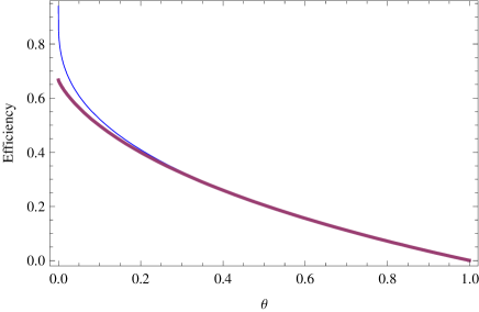
Figure 1: The efficiency in Eq. (35) and (40) are plotted versus $\theta$. The lower curve (thick line) is the efficiency at maximum power for the Brownian heat engine. The upper curve is the efficiency obtained from the classical model with intermediate temperature as the single uncertain parameter. The same expected efficiency is also obtained in the asymptotic limit of the quantum model when two intrinsic energy scales of the working medium are uncertain.

The similarity between Eqs. (39) and (41) up to the second order, suggests there might be a new universality class which includes these efficiencies. In Fig. 1, the efficiencies given in (35) and (40) are plotted. To conclude, when all the unknown parameters are treated with prior probabilities, the expected behavior of quantum model with two internal energy scales as the uncertain parameters is similar to the classical model with intermediate temperature as the single uncertain parameter. Interestingly, the expected efficiency in both cases, approaches $\eta_{c}/3$ value, in the near-equilibrium limit. Further, the analysis based on subjective treatment of the incomplete information, suggests a new line of enquiry of a possible connection with optimal performance of the finite time irreversible models of heat engines.

VII Acknowledgements

RSJ thanks the organizers of FQMT-2011 conference and in particular, Prof. Theo M. Nieuwenhuizen and Prof. Vaclav Spicka for the invitation to Prague. RSJ is supported by Department of Science and Technology, India under the project No. SR/S2/CMP-0047/2010(G). GT thanks IISER Mohali for research fellowship. PA is supported by UGC through Junior research fellowship.

References

- (1) M.O. Scully, Phys. Rev. Lett. 87, 220601 (2001).
- (2) M.O. Scully, M.S. Zubairy, G.S. Agarwal, and H. Walther, Science 299, 862 (2003).
- (3) T. D. Kieu, Phys. Rev. Lett. 93, 140403 (2004); Eur. Phys. J. D 39, 115 (2006).
- (4) R. Dillenschneider and E. Lutz, Europhys.Lett. 88, 5003(2009).
- (5) N. Linden, S. Popescu, and P. Skrzypczyk, Phys. Rev. Lett. 105, 130401 (2010).
- (6) R.S. Johal, Phys. Rev. E 82, 061113 (2010).
- (7) G. Thomas and R.S. Johal, Phys. Rev. E 83, 031135 (2011).
- (8) G. Thomas and R.S. Johal, Phys. Rev. E 85 041146 (2012).
- (9) H. Jeffreys, Theory of Probability (2nd edition, Clarendon Press, Oxford, 1948).
- (10) E.T. Jaynes, IEEE Trans. Sys. Sc. and Cybernetics, 4, 227 (1968).
- (11) G. N. Hatsopoulos and E. P. Gyftopoulos, Found. Phys. 6, 127 (1976).
- (12) A. E. Allahverdyan, R. Balian, and Th. M. Nieuwenhuizen, J. Mod. Opt. 51, 2703 (2004).
- (13) A. E. Allahverdyan, R. S. Johal, and G. Mahler, Phys. Rev. E 77, 041118 (2008).
- (14) F. Curzon and B. Ahlborn, Am. J. Phys. 43, 22 (1975).
- (15) Z.C. Tu, J. Phys. A: Math. Theor. 41, 312003 (2008).
- (16) M. Esposito et. al., Phys. Rev. Lett. 105, 150603 (2010).
- (17) Y. Zhang, B.H. Lin, and J.C. Chen, Eur. Phys. J. B 53, 481 (2006).