Abstract

A class of models is introduced describing the evolution of population species whose carrying capacities are functionals of these populations. The functional dependence of the carrying capacities reflects the fact that the correlations between populations can be realized not merely through direct interactions, as in the usual predator-prey Lotka-Volterra model, but also through the influence of species on the carrying capacities of each other. This includes the self-influence of each kind of species on its own carrying capacity with delays. Several examples of such evolution equations with functional carrying capacities are analyzed. The emphasis is given on the conditions under which the solutions to the equations display extreme events, such as finite-time death and finite-time singularity. Any destructive action of populations, whether on their own carrying capacity or on the carrying capacities of co-existing species, can lead to the instability of the whole population that is revealed in the form of the appearance of extreme events, finite-time extinctions or booms followed by crashes.

PACS: 02.30.Hq, 02.30.Ks, 87.10.Ed, 87.23.Ce, 87.23.Cc, 87.23.Ge, 87.23.Kg, 89.65.Gh

Keywords: Population evolution, Functional carrying capacity, Punctuated solution, Models of symbiosis, Nonlinear differential equations, Extreme events, Finite-time death, Finite-time singularity, Evolutional booms and crashes

1 Brief survey of population models

Evolution equations, describing population dynamics, are widely employed in various branches of biology, ecology, and sociology. The main forms of such equations are given by the variants of the predator-prey Lotka-Volterra models. In this paper, we introduce a novel class of models whose principal feature, making them different from other models, is the functional dependence of the population carrying capacities on the population species. This general class of models allows for different particular realizations characterizing specific correlations between coexisting species. The functional dependence of the carrying capacities describes the mutual influence of species on the carrying capacities of each other, including the self-influence of each kind of species on its own capacity. Such a dependence is, both mathematically and biologically, principally different from the direct interactions typical of the predator-prey models. Before formulating the general approach, we give in this section a brief survey of the main known models of population dynamics. This will allow us to stress the basic difference of our approach from other models used for describing the population dynamics in biology, ecology, and sociology.

(i) Predator-prey Lotka-Volterra model

The first model, describing interacting species, one of which is a predator with population $N_{1}$, and another is a prey with population $N_{2}$, has been the Lotka-Volterra [1, 2] model

$$\frac{dN_{1}}{dt}=-\gamma_{1}N_{1}+A_{12}N_{2}N_{1}\;,\qquad\frac{dN_{2}}{dt}=\gamma_{2}N_{2}-A_{21}N_{1}N_{2}\;,$$ (1)

where all coefficients are positive numbers. It is easy to show that the solutions to these equations are bound oscillating functions of time.

(ii) Predator-prey Kolmogorov model

The Lotka-Volterra model is a particular case of the predator-prey Kolmogorov model [3, 4] that has the general form

$$\frac{dN_{1}}{dt}=f_{1}(N_{1},N_{2})N_{1}\;,\qquad\frac{dN_{2}}{dt}=f_{2}(N_{1},N_{2})N_{2}\;,$$ (2)

under the conditions

$$\frac{\partial f_{1}}{\partial N_{2}}\;>\;0\;,\qquad\frac{\partial f_{2}}{\partial N_{1}}\;<\;0\;.$$

This model is too general and requires specifications for describing concrete cases.

(iii) Generalized predator-prey Lotka-Volterra model

Generalizing the Lotka-Volterra model (1) to multiple species yields the equations

$$\frac{dN_{i}}{dt}=\left(\gamma_{i}+\sum_{j}A_{ij}N_{j}\right)N_{i}\;,$$ (3)

where all coefficients are real numbers [5]. The signs of the parameters can be different. When all $\gamma_{i}$’s are positive, while all $A_{ij}$’s are negative, one gets the competitive Lotka-Volterra equations whose behavior has been analyzed in detail in Refs. [6, 7, 8, 9].

(iv) Replicator equations

These equations have the form

$$\frac{dN_{i}}{dt}=\left(f_{i}-\overline{f}\right)N_{i}\;,$$ (4)

where $f_{i}$ is the species fitnesses and

$$\overline{f}\equiv\sum_{i}f_{i}N_{i}$$

is the average fitness characterizing the whole society [5]. The species populations are usually assumed to be defined on a simplex, being normalized to a constant representing the total fixed population

$$\sum_{i}N_{i}=N=const\;.$$

The $n$- dimensional replicator model is equivalent to the $n-1$-dimensional Lotka-Volterra model (3), to which it can be reduced by a change of variables [5, 10].

(v) Jacob-Monod equations

The equations describe not the coexisting species but rather a single type of species of population $N_{1}$, like bacteria, which are fed on the nutrient of amount $N_{2}$. The nutrient plays the role of the prey that is getting depleted being consumed by the feeders and, at the same time, being supplied into the system from outside according to the supply function $f(N_{2})=\alpha N_{2}/(\beta+N_{2})$. The equations read as

$$\frac{dN_{1}}{dt}=f(N_{2})N_{1}\;,\qquad\frac{dN_{2}}{dt}=-\gamma f(N_{2})N_{1},$$ (5)

with all parameters being positive [11]. As time increases, $t\rightarrow\infty$, the nutrient becomes depleted, $N_{2}\rightarrow 0$, and the bacteria population reaches the stationary value $N_{1}=N_{1}(0)+N_{2}(0)/\gamma$.

The Holling equation of second kind [12] takes into account that predators, in order to consume prey, need to search for it, chase, kill, eat, and digest. This is why predators attack not all preys but a limited number of them, which saturates to a constant when the prey density increases. Mathematically, the Holling equation is analogous to the Jacob-Monod model.

(vi) Verhulst logistic equation

The well known logistic equation

$$\frac{dN}{dt}=\gamma N\left(1\;-\;\frac{N}{K}\right)\;,$$ (6)

where all parameters are positive, was suggested by Verhulst [13]. The constant $K$ is the carrying capacity. The solution to this equation is the sigmoid function

$$N(t)=\frac{N_{0}Ke^{\gamma t}}{K+N_{0}\left(e^{\gamma t}-1\right)}\;,$$

in which $N_{0}\equiv N(0)$.

(vii) Hutchinson delayed logistic equation

If one interprets the term inside the brackets in Eq. (6) as an effective reproductive rate, then, as Hutchinson argued [14], it could be delayed in time, which results in the equation

$$\frac{dN(t)}{dt}=\gamma N(t)\left[1\;-\;\frac{N(t-\tau)}{K}\right]\;,$$ (7)

in which $K$ is a fixed carrying capacity. The solution to this equation gives additional oscillations superimposed on the logistic curve.

(viii) Generalized delayed logistic equations

There are many variants generalizing the delayed logistic equation (7), which can be found in Refs. [15, 16, 17]. For example, the multiple-delayed equation

$$\frac{dN(t)}{dt}=\gamma N(t)\left[1\;-\sum_{j}\;\frac{N(t-\tau_{j})}{K_{j}}\right]\;,$$ (8)

where the carrying capacities $K_{j}$ are positive constants. All such equations are usually applied to single-species systems of population $N$. The multiple carrying capacities $K_{j}$ in Eq. (8) correspond to different processes of the same single species. The logistic equations of the above type, whether with delays or without them, do not describe the possible coexistence of several species. When such equations are generalized to the case of several species, one comes back to the generalized Lotka-Volterra predator-prey model (3).

(ix) Peschel-Mende hyperlogistic equation

In order to take into account the accelerated growth of population, occurring, for instance, for the human world population, Peschel and Mende [18] extended the standard logistic equation by introducing two additional positive powers $m$ and $n$, getting the equation

$$\frac{dN}{dt}=\gamma N^{m}\left(1\;-\;\frac{N}{K}\right)^{n}\;.$$ (9)

The solution to this equation could be reasonably well fitted to the world population dynamics. The form of the solution is a slightly modified sigmoid curve, with the population never surmounting the carrying capacity $K$. For $m=1$ and $n=1$, the Verhulst logistic equation (6) is recovered.

(x) Hyperlogistic time-delay equations

The straightforward extension of the Peschel-Mende hyperlogistic equation is the hyperlogistic time-delay equation

$$\frac{dN(t)}{dt}=\gamma N^{m}(t)\left[1\;-\;\frac{N(t-\tau)}{K}\right]^{n}\;,$$ (10)

which can also be treated as a generalization of the Hutchinson delayed logistic equation (7). This time-delay equation is capable of simulating a population that can essentially surmount the carrying capacity $K$ for a limited period of time, then dropping below it subsequently [19].

(xi) Singular Malthus equations

All equations enumerated above produce bounded solutions. In some cases, the population dynamics seems to follow a law ending with divergent solutions. The well known Malthus equation [20] gives the exponential population growth. But sometimes, the population dynamics develops a super-exponential behavior, diverging at a finite time $t_{c}$ according to a power law of the time to the singular time $t_{c}$. The simplest way of modeling such a behavior is by the equation

$$\frac{dN}{dt}=\gamma N^{m}\;,$$ (11)

with the power $m\geq 1$. This is a direct generalization of the Malthus equation, capturing the positive feedback of the population on the growth rate: the larger the population, the higher the growth rate. For $m=1$, one recovers the usual Malthus equation with the exponential solution. When $m>1$, the solution to the equation (11) is of power law

$$N(t)=\frac{C}{(t_{c}-t)^{1/\varepsilon}}\;,$$

where

$$C\;\equiv\;\frac{1}{(\varepsilon\gamma)^{1/\varepsilon}}\;,\qquad\varepsilon\equiv m-1\;,$$

$$t_{c}\;\equiv\;\frac{1}{N^{\varepsilon}_{0}\varepsilon\gamma}\;,\qquad N_{0}\equiv N(0)\;.$$

The solution diverges hyperbolically at the critical time $t_{c}$. Such strongly singular solutions were first discussed by von Foerster et al. [21] and applied to rationalize the super-exponential growth of the human world population [22, 23, 24, 25], population dynamics and financial markets [26, 27, 28], material failures and earthquakes [29, 30], climate and environmental changes [31, 32, 33, 34], and dynamics of other systems [35, 36, 37]. In ecology, the correlation between population density and the per capita growth rate is known as the Allee effect [38]. The feedback between the population density, associated with the Allee effect, can lead to the increase of the effective growth rate, in the case of sufficiently large populations, or to the rate decrease and species extinction for small-density populations [38, 39, 40, 41].

In addition to the differential equations describing population dynamics, there exist as well difference equations [42, 43] and integro-differential equations [44, 45]. There are more complicated equations characterizing several factors, such as the population density, mass or weight dependence of individual members of different species, the dynamics of available food, and so on [44, 46, 47]. Some study the influence on population dynamics of available information [48]. It is also possible to investigate the spatial dependence of populations [49]. More details on these and other types of equations can be found in the review articles [50, 51, 52, 53].

We do not consider here the complications caused by the desire to take into account many various features of the studied populations. Our aim here is different: we concentrate our attention on the influence of the functional dependence of carrying capacities on population densities. Since this idea is rather new, it is necessary, first of all, to study the related effects for simpler equations, without overloading them by secondary specifications. Once the main influence of the functional carrying capacities is understood, it will be possible to complicate the equations by taking into account more and more mechanisms and specificities. For the same reason, the parameters characterizing the interactive species are treated as fixed. In reality, the characteristics of each given biological species vary in general with the age of the individuals composing the group. However, it is always admissible to divide the populations into different age ranges characterized by similar birth and death rates. Another possibility is to consider each species being characterized by effective averaged parameters, which corresponds to what is called the mean-field approximation [36, 37, 54].

In the dynamics of any population, one can distinguish several time scales. The shortest time scale is the interaction time $t_{int}$, describing interactions between individuals. This time is much shorter than the observation time $t_{obs}$, during which the population is investigated. In order that the studied species could be characterized by fixed parameters, such as birth-death rates, the observation time should be shorter than the variation time $t_{var}$ during which individuals experience noticeable changes related, e.g., to their age. In this way, we keep in mind the situation, when

$$t_{int}\ll t_{obs}\ll t_{var}\;.$$

Then all population parameters, except the carrying capacity, can be kept fixed. Our main point is that the carrying capacity can vary due to mutual interactions of individuals, hence it varies during the interaction time and this variation needs to be taken into account.

The standard situation in treating the population evolution by means of the equations of the above types is that the carrying capacities are kept as fixed constant parameters. In the following Section 2, we propose an approach where the carrying capacities are functionals of the species populations. This makes it possible to drastically extend the applicability of the population-evolution equations to various situations describing the regimes that where unavailable with other models. The basic idea of the approach has been formulated in our previous papers [39, 40], where some particular models were considered. Now, in Section 2, we propose a general framework for generating a large class of such models. In Sections 3 and 4, we consider particular variants of the suggested equations, corresponding to those of Refs. [39, 40]. The difference from the previous works is three-fold. First, we simplify the consideration by a convenient choice of the scaling for the terms describing the carrying capacities, which allows us to make a more straightforward classification of different dynamical regimes. Second, we emphasize the conditions under which solutions arise that are characterized by extreme events, such as the finite-time death and finite-time singularity of the species. Third, we suggest a new interpretation for an extreme event such as the finite-time singularity. The novel interpretation is based on the leverage effect and considers the singularity as a manifestation of an evolutional boom followed by a crash. Our considerations are phrased for applications to the development, growth and possible collapse of biological as well as human societies, as they both follow similar dynamics with analogous underlying mechanisms [37].

2 Population evolution with functional carrying capacity

The idea that the carrying capacity may be not a constant but a function of population fractions has repeatedly appeared in the literature in the form of general discussions. In Sec. 2.1, we give a historical overview of these ideas that provide a firm justification for their mathematical representation in Sec. 2.2 and in the following sections.

2.1 General meaning of functional carrying capacity

The carrying capacity of a biological species in an environment is generally understood as the maximum population size of the species that the environment can sustain indefinitely, given the food, habitat, water and other necessities available in the environment. In population biology, carrying capacity is defined as the environment maximal load [55], which is different from the concept of population equilibrium. Historically, carrying capacity has been treated as a given fixed value [56, 57]. But then, it has been understood that the carrying capacity of an environment may vary for different amounts of species and may change over time due to a variety of factors, including food availability, water supply, environmental conditions, living space, and population activity.

Thus, the carrying capacity of a human society is influenced by the intensity of human activity, which depends on the level of technological development. When prehistoric humans first discovered that crude tools and weapons allowed greater effectiveness in gathering wild foods and hunting animals, they effectively increased the carrying capacity of the environment for their species. The subsequent development and improvement of agricultural systems has had a similar effect, as have discoveries in medicine and industrial technology. Clearly, the cultural and technological evolution of human socio-technological systems has allowed enormous increases to be achieved in carrying capacity for our species. This increased effectiveness of environmental exploitation has allowed a tremendous multiplication of the human population to occur [58, 59].

Technology is an important factor in the dynamics of carrying capacity. For example, the Neolithic revolution increased the carrying capacity of the world relative to humans through the invention of agriculture. Currently, the use of fossil fuels has artificially increased the carrying capacity of the world by the use of stored sunlight, albeit with increasingly negative externalities, such as global warming, ocean acidification and the indirect reduction of diversity. Other technological advances that have increased the carrying capacity of the world relative to humans are: polders, fertilizer, composting, greenhouses, land reclamation, and fish farming. Agricultural capability on Earth expanded in the last quarter of the 20th century. Whether this is sustainable is debatable. There are signs that human-induced soil erosion as well as destabilization of sensitive ecosystems may lead, at the same time, to a reduction of agricultural capability over the coming decades, such as in Africa where the population is expected to double before 2050. The change in the carrying capacity of the habitat and environment supporting a human society can be described by the consumption impact [60], which is proportional to the population size, with a coefficient characterizing the technology level.

One way to estimate human influence on the carrying capacity of the ecosystem is to use the so-called ecological footprint accounting method that provides empirical, non-speculative assessments of human activities with regard to the preservation or destruction of the Earth carrying capacity. It compares regeneration rates (biocapacity) against human demand (ecological footprint) in the same year. The results show that, in recent years, humanity demand has exceeded the planet biocapacity by more than 20 percent [61]. The present situation of rapid population growth in some regions, massive overexploitation of resources and steady accumulation of pollution and wastes diminishes the Earth carrying capacity. To a first approximation, with all the caveats associated with the heterogeneity of technological developments in different parts of the World, one can consider an average footprint per person, which leads to an estimation of the decrease of the Earth carrying capacity as roughly proportional to the size of the total population. The question is how and by what means this change of the Earth carrying capacity for humanity will pay back [62].

Mutual coexistence and symbiosis of several species also strongly influences the carrying capacities of the species, with the changes being, to a first approximation, proportional to the species numbers. For example, humans have increased the carrying capacity of the environment for a few other species, including those with which we live in a mutually beneficial symbiosis. Those companion species include more than about 20 billion domestic animals such as cows, horses, pigs, sheep, goats, dogs, cats, and chickens, as well as certain plants such as wheat, rice, barley, maize, tomato, and cabbage. Clearly, humans and their selected companions have benefited greatly through active management of mutual carrying capacities [63].

Interactions between two or more biological species are known to essentially influence the carrying capacity of each other, by either increasing it, when species derive a mutual benefit, or decreasing it, when their interactions are antagonistic [64, 65, 66]. The same applies to economic and financial interactions between firms, which also form a kind of symbiosis, where the interacting firms develop the carrying capacity of each other also roughly proportionally to their sizes [67].

Many authors (e.g., Del Monte-Luna et al. [68]) stress that, due to the influence on the carrying capacity resulting from the existing populations, its original definition implying a constant value has lost its meaning. As a consequence of the feedback loops of the population sizes, the notion of carrying capacities has taken a broader sense. Carrying capacity should be understood as a non-equilibrium relationship or function that depends on the population size and on the symbiotic relations between the interacting populations. It characterizes the growth or development of available resources at all hierarchical levels of biological integration, beginning with the populations, and shaped by processes and interdependent relationships between finite resources and the consumers of those resources [68].

The above discussion shows that, in general, the carrying capacity is not a fixed quantity, but it should be considered a function of population sizes. In the case of a single species, the carrying capacity can be created or destroyed by the species activity. The simplest assumption is to take the species impact as proportional to the species population size. When species coexist, their carrying capacities are influenced by the species mutual interactions, either facilitating the capacity development or damaging it. Being functions of the species populations, such nonequilibrium carrying capacities can be naturally represented as polynomials over the population numbers [69].

2.2 Mathematical formulation of basic equations

Let the considered society consist of several species enumerated by an index $i=1,2,\ldots$. The number of members in a society is denoted as $N_{i}=N_{i}(t)$,

The main idea of our approach is that the carrying capacity of each species is not a fixed constant, but it is a functional

$$K_{i}=K_{i}(\{N_{i}\})$$ (12)

of the set $\{N_{i}\}$ of the species populations. This assumption takes into account that the species may interact not merely directly but also by influencing the carrying capacities of each other as well as their own carrying capacity.

A general form of the evolution equations, that takes into account both direct interactions and mutual influence on the carrying capacities, can be written as

$$\frac{dN_{i}}{dt}=\left(\gamma_{i}+\sum_{ij}\frac{C_{ij}}{K_{i}}\;N_{j}\right)N_{i}\;,$$ (13)

where $K_{i}$ is the functional carrying capacity (12). If the latter were a fixed parameter, one would return to the generalized Lotka-Volterra predator-prey model (3). But in our approach, the carrying capacities are nontrivial functionals of populations.

In a particular case, when the species do not display strong direct interactions, but their mutual correlations are mainly through influencing the carrying capacities of each other, then Eq. (13) reduces to the evolution equation

$$\frac{dN_{i}}{dt}=\gamma_{i}N_{i}\;-\;\frac{C_{i}N_{i}^{2}}{K_{i}}\;.$$ (14)

Here the effective rate

$$\gamma_{i}\equiv\gamma_{i}^{birth}-\gamma_{i}^{death}$$ (15)

is the difference between the birth and death rates of the corresponding species. When birth prevails over death, then $\gamma_{i}>0$, while if death is prevailing over birth, then $\gamma_{i}<0$. In economic applications, birth translates into gain and death into loss. The parameter

$$C_{i}\equiv C_{i}^{comp}-C_{i}^{coop}$$ (16)

characterizes the difference between the competition and cooperation of the members inside a given type of species. When competition is stronger than cooperation, then $C_{i}>0$, while if cooperation is stronger, then $C_{i}<0$.

It is important to stress that Eq. (13) is principally different, both mathematically as well as by its meaning, from the predator-prey model (3). Similarly, Eq. (14) is principally different from the logistic equation (6) or its variants (7) and (8). As a result, the equations with functional carrying capacities can display novel types of solutions allowing for the consideration of effects that are absent in other evolution equations. In the following sections, we consider concrete examples of evolution equations with functional carrying capacities.

3 Action of society on its own carrying capacity

3.1 Justification for equation form

In the previously studied variants of the logistic equation, the carrying capacity is treated as a given quantity. However, it is often the case that the society activity does influence its own carrying capacity that can be either enhanced by producing new goods, materials, knowledge, and so on, or can be destroyed by unreasonable exploitation of resources, e.g., by deforestation, polluting water, and spoiling climate. Therefore, the carrying capacity, taking into account such feedback effects, must be a functional $K=K(N)$ of the population $N$.

Thus, the population evolution is characterized by the equation

$$\frac{dN}{dt}=\gamma N\;-\;\frac{CN^{2}}{K(N)}\;,$$ (17)

with the carrying capacity depending on $N$ itself.

Moreover, the creation or destruction of the carrying capacity by the society members does not occur immediately, but is delayed since any creation or destruction requires time for its realization. Hence, the variable $N$, entering the carrying capacity, should be delayed in time by a lag $\tau$, so that $K(N)=K(N(t-\tau))$.

Different types of carrying capacity can be introduced that depend on a delayed population variable. In the present paper, we consider a simple linear form

$$K(N)=A+BN(t-\tau)\;.$$ (18)

Here the first term $A>0$ is a natural carrying capacity, provided by Nature. The second term is the created or destroyed capacity, depending on whether the society activity is constructive or destructive. The parameter $B$ is the production factor, if it is positive, and it is a destruction factor, when it is negative. Form (18) of the carrying capacity agrees with the assumption of additivity, when its different parts sum to produce the total carrying capacity.

3.2 Reduced quantities and choice of scaling

As the population numbers can be very large, it is therefore more convenient to deal with the reduced quantities

$$x\equiv\frac{N(t)}{N_{eff}}$$ (19)

measured in units of some typical population size $N_{eff}$. It is also convenient to introduce dimensionless parameters for the natural carrying capacity

$$a\equiv\frac{A}{N_{eff}}\left|\;\frac{\gamma}{C}\;\right|$$ (20)

and for the production-destruction factor

$$b\equiv B\left|\;\frac{\gamma}{C}\;\right|\;.$$ (21)

The total dimensionless carrying capacity

$$y\equiv\frac{K(N)}{N_{eff}}\left|\;\frac{\gamma}{C}\;\right|$$ (22)

takes the form

$$y=a+bx(t-\tau)\;.$$ (23)

Up to now, the effective value $N_{eff}$ has been arbitrary. By a special choice of the scaling, it is possible to simplify the equations and to make a more transparent classification of arising dynamical regimes. It is convenient to choose

$$N_{eff}\equiv A\left|\;\frac{\gamma}{C}\;\right|\;.$$ (24)

Then parameters (20) and (21) reduce to

$$a=1\;,\qquad b=\frac{B}{A}\;N_{eff}\;.$$ (25)

The dimensionless carrying capacity (23) becomes

$$y=1+bx(t-\tau)\;.$$ (26)

Let us also define the signs of the birth-death rate and of the competition-cooperation parameter as

$$\sigma_{1}\equiv{\rm sgn}\gamma=\frac{\gamma}{|\gamma|}\;,\qquad\sigma_{2}\equiv{\rm sgn}C=\frac{C}{|C|}\;.$$ (27)

Depending on these signs, the following situations can occur.

$$\begin{array}[]{lll}\sigma_{1}=+1\;,&~{}\sigma_{2}=+1&~{}(gain\;+\;competition)\;,\\ \sigma_{1}=+1\;,&~{}\sigma_{2}=-1&~{}(gain\;+\;cooperation)\;,\\ \sigma_{1}=-1\;,&~{}\sigma_{2}=+1&~{}(loss\;+\;competition)\;,\\ \sigma_{1}=-1\;,&~{}\sigma_{2}=-1&~{}(loss\;+\;cooperation)\;.\end{array}$$ (32)

Using the above notations and measuring time $t>0$ in units of $1/\gamma$, we reduce Eq. (17) to

$$\frac{dx}{dt}=\sigma_{1}x-\sigma_{2}\;\frac{x^{2}}{y}\;,$$ (33)

with the carrying capacity (26). This equation is to be complemented by the initial conditions

$$x(t)=x_{0}\qquad(t\leq 0)\;,$$

$$y(t)=y_{0}=1+bx_{0}\qquad(t\leq 0)\;.$$ (34)

The solution for $x$, by its meaning, is to be positive. The production-destruction factor $b$ can take any real values, being positive for the constructive society activity, while negative, for its destructive activity.

3.3 Evolutionary stable states

One of the most important problems in studying any evolutional model is the determination of evolutionary stable states. These are given by the stable stationary solutions to the considered equation. In order to analyze the stability of the solutions to the differential delay equations, we employ the Lyapunov stability theory following the work by Pontryagin [70] and the books [11, 15, 16].

The stationary states of Eq. (33) are defined as the solutions to the fixed-point equation

$$\sigma_{1}x^{*}\;-\;\frac{\sigma_{2}(x^{*})^{2}}{1+bx^{*}}=0\;.$$ (35)

This yields two fixed points

$$x_{1}^{*}=0\;,\qquad x_{2}^{*}=\frac{\sigma_{1}}{\sigma_{2}-b}\;.$$ (36)

Resorting to the Lyapunov stability analysis, we need to consider a small deviation

$$\delta x_{j}(t)=x_{j}(t)-x_{j}^{*}\qquad(j=1,2)$$ (37)

from the related fixed point. This deviation satisfies the equation

$$\frac{d}{dt}\;\delta x_{j}(t)=C_{j}\delta x_{j}(t)+D_{j}\delta x_{j}(t-\tau)\;,$$ (38)

in which

$$C_{j}\equiv\sigma_{1}\;-\;\frac{2\sigma_{2}x_{j}^{*}}{1+bx_{j}^{*}}\;,\qquad D_{j}\equiv b\sigma_{2}\frac{x_{j}^{*}}{1+bx_{j}^{*}}\;.$$

For the corresponding fixed points, these parameters are

$$C_{1}=\sigma_{1}\;,\qquad D_{1}=0\;,$$

$$C_{2}=\sigma_{1}\;\frac{b(\sigma_{1}-1)-\sigma_{2}}{b(\sigma_{1}-1)+\sigma_{2}}\;,\qquad D_{2}=\frac{b\sigma_{2}}{[b(\sigma_{1}-1)+\sigma_{2}]^{2}}\;.$$

Looking for the deviation in the exponential form

$$\delta x_{j}(t)\;\propto\;e^{\lambda_{j}t}\;,$$

we obtain the equation

$$\lambda_{j}=C_{j}+D_{j}e^{-\lambda_{j}\tau}$$ (39)

for the characteristic exponents $\lambda_{j}$. By using the notation

$$W_{j}\equiv(\lambda_{j}-C_{j})\tau\;,\qquad z_{j}\equiv\tau D_{j}e^{-C_{j}\tau}\;,$$

equation (39) becomes

$$W_{j}e^{W_{j}}=z_{j}\;,$$

which is nothing but the equation defining the Lambert function $W_{j}$. Therefore, the characteristic-exponent equation (39) acquires the form

$$\lambda_{j}=C_{j}+{1\over\tau}W_{j}(D_{j}e^{-C_{j}\tau})\;.$$ (40)

The stationary solution is stable when the real part of the characteristic exponent is negative, $\Re\lambda_{j}<0$.

To proceed further, we shall analyze separately the cases listed in Eq. (32).

4 Society with gain and competition

Under the prevailing gain (birth) and competition, when

$$\sigma_{1}=1\;,\qquad\sigma_{2}=1\;,$$ (41)

the evolution equation (33) reads as

$$\frac{dx(t)}{dt}=x(t)\;-\;\frac{x^{2}(t)}{1+bx(t-\tau)}\;.$$ (42)

At the initial stage, when $0\leq t<\tau$, we have the exact solution

$$x(t)=\frac{x_{0}(1+bx_{0})e^{t}}{1+x_{0}(b-1+e^{t})}\qquad(0\leq t<\tau)\;.$$

This can be used for constructing by iteration an approximate solution at the second stage, when $\tau<t<2\tau$. Then we could find an approximate solution at the third step, and so on. However, the accuracy of such iterative constructions quickly deteriorates and is admissible only over a couple of initial steps. More accurate solutions are to be found by numerically solving the evolution equation (42).

The stability analysis of the previous section shows that the fixed point $x_{1}^{*}=0$ is unstable for all $b$ and $\tau$. The second fixed point

$$x_{2}^{*}=\frac{1}{1-b}\equiv x^{*}$$ (43)

is stable when either

$$-1<b<1\;,\qquad\tau\geq 0\;,$$ (44)

or when

$$b<-1\;,\qquad\tau\leq\tau_{0}\;,$$ (45)

where

$$\tau_{0}\equiv\frac{1}{\sqrt{b^{2}-1}}\;\arccos\left(\frac{1}{b}\right)\;.$$ (46)

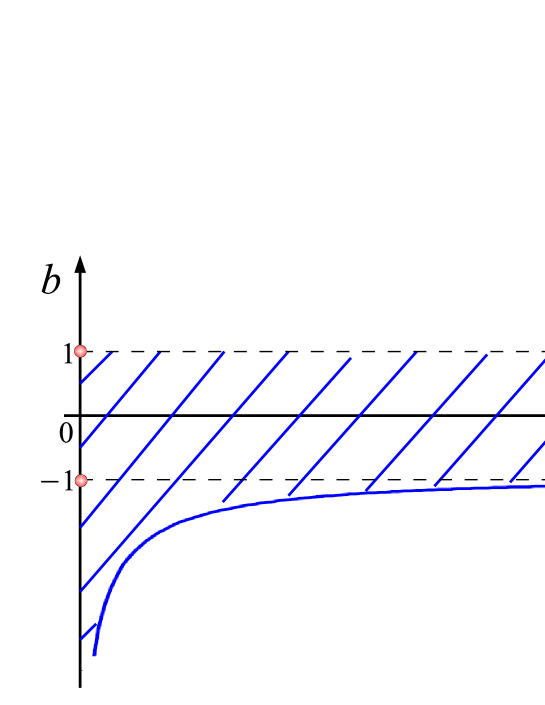
Figure 1: Stability region for the gain-competition case defined in (41).

The stability region is shown in Fig. 1.

Varying the system parameters and initial conditions, we can meet the following dynamic regimes.

4.1 Punctuated unlimited growth

For the parameters

$$b\geq 1\;,\qquad\tau\geq 0\qquad(x_{0}>0)\;,$$ (47)

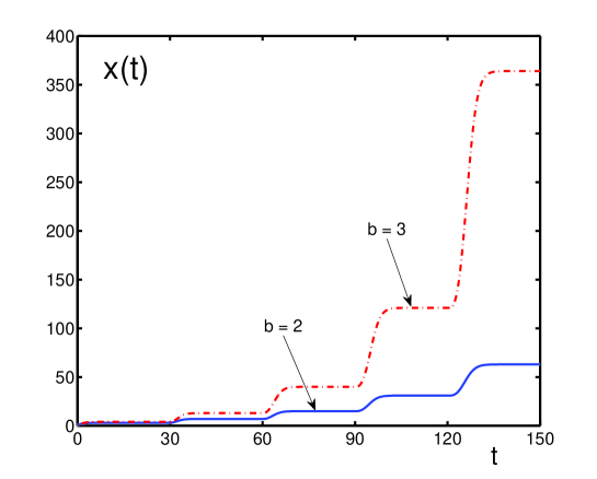
Figure 2: Temporal behavior of solutions to equation (42) for the initial condition $x_{0}=1$, lag $\tau=30$, and parameters $b=2$ (solid line) and $b=3$ (dashed-dotted line). Solutions $x(t)\rightarrow\infty$, when $t\rightarrow\infty$.

the population grows by steps, as shown in Fig. 2. The growth continues to infinite times. This is a typical example of the punctuated evolution caused by the fact that the production factor $b$ is positive and sufficiently large. Hence, the carrying capacity is produced by the population, with a delay $\tau$.

4.2 Punctuated growth to stationary state

The punctuated growth is not always unbounded, but it can be bounded by the fixed point, provided the initial condition $x_{0}$ is smaller than $x^{*}$ and the parameters are

$$0\leq b<1\;,\qquad\tau\geq 0\qquad\left(x_{0}<x^{*}\right).$$ (48)

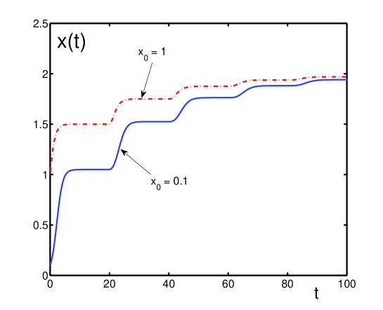
Figure 3: Dynamics of solutions to equation (42) for the lag $\tau=20$, symbiotic parameter $b=0.5$, and the initial conditions $x_{0}=0.1$, (solid line) and $x_{0}=1$ (dashed-dotted line). Solutions $x(t)\rightarrow x^{*}$, monotonically growing by steps, when $t\rightarrow\infty$. The stationary point is $x^{*}=1/(1-b)=2$.

This regime is presented in Fig. 3.

4.3 Punctuated decay to stationary state

When the parameters are the same as in Eq. (48), but the initial condition $x_{0}$ is larger than the fixed point $x^{*}$,

$$x_{0}>x^{*}=\frac{1}{1-b}\;,$$ (49)

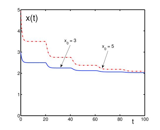
Figure 4: Evolution of solutions to equation (42) for the lag $\tau=20$, parameter $b=0.5$, and initial conditions $x_{0}=3$, (solid line) and $x_{0}=5$ (dashed-dotted line). Solutions $x(t)\rightarrow x^{*}$, monotonically diminishing by steps, when $t\rightarrow\infty$. The stationary point is $x^{*}=1/(1-b)=2$, the same as in Fig. 3.

then there appears the punctuated decay, as illustrated in Fig. 4.

4.4 Punctuated alternation to stationary state

If the carrying capacity is destroyed by the population, then there can occur a punctuated alternation to a stationary state, when the parameters and the initial condition are

$$-1\leq b<0\;,\qquad\tau\geq 0\qquad\left(x_{0}<\frac{1}{|b|}\right)\;.$$ (50)

This is depicted in Fig. 5.

4.5 Oscillatory approach to stationary state

For sufficiently large destruction factor, there arises a regime of an oscillatory approach to a stationary state, as is presented in Fig. 6. This happens under the parameters and the initial condition being defined by the inequalities

$$b<-1\;,\qquad\tau<\tau_{0}\qquad\left(x_{0}<\frac{1}{|b|}\right)\;,$$ (51)

where the lag $\tau_{0}$ is defined in Eq. (46).

4.6 Sustained oscillations

There exists a lag $\tau_{1}=\tau_{1}(b)$, such that, when

$$b<-1\;,\qquad\tau_{0}\leq\tau\leq\tau_{1}\qquad\left(x_{0}<\frac{1}{|b|}\right)\;,$$ (52)

then oscillations do not decay, but continue without attenuation, as in Fig. 7. The lag $\tau_{1}(b)$ can be found only numerically.

4.7 Punctuated alternation to finite-time death

If the time lag surpasses the value $\tau_{1}=\tau_{1}(b)$, the alternating solution exists only for a limited time. At the death time $t_{d}$, given by the equation

$$1+bx(t_{d}-\tau)=0\;,$$ (53)

all population becomes extinct, as in Fig. 8. This happens for the parameters

$$b<-1\;,\qquad\tau>\tau_{1}\qquad\left(x_{0}<\frac{1}{|b|}\right)\;.$$ (54)

4.8 Growth to finite-time singularity

In the case, where the activity of the population is destructive, time lags are large, and the initial condition is also large, so that

$$b<0\;,\qquad\tau>\tau_{c}\qquad\left(x_{0}>\frac{1}{|b|}\right)\;,$$ (55)

the population dynamics becomes dramatic, diverging at a finite time, called the critical time. The divergence is hyperbolic, according to the law

$$x(t)\;\propto\;\frac{1}{t_{c}-t}\qquad(t\rightarrow t_{c}-0)\;,$$ (56)

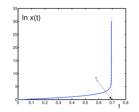
Figure 9: Behavior of the solution to equation (42) in logarithmic scale for the parameter $b=-2<-1$, lag $\tau=1.7>\tau_{1}$, where $\tau_{1}\approx 1.65$ is defined numerically, and the initial condition $x_{0}=1>1/|b|$. Solution $x(t)$ diverges, $x(t)\rightarrow\infty$, when $t\rightarrow t_{c}\approx 0.69315$.

as is demonstrated in Fig. 9. The values of the critical lag $\tau_{c}$ and the critical divergence time $t_{c}$ can be found numerically.

4.9 Unlimited exponential growth

For shorter time lags, when

$$b<0\;,\qquad\tau\leq\tau_{c}\qquad\left(x_{0}>\frac{1}{|b|}\right)\;,$$ (57)

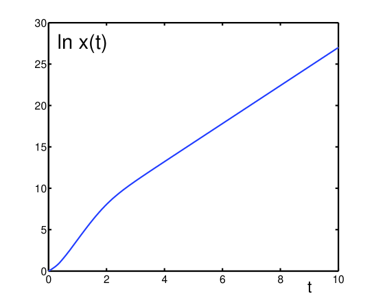
Figure 10: Behavior of the solution, shown in logarithmic scale, to equation (42) for the parameter $b=-2<-1$, lag $\tau=0.415<\tau_{c}$, where $\tau_{c}\approx 0.416$ is defined numerically, with the initial condition $x_{0}=1>1/|b|$. Solution $x(t)$ exponentially grows, when $t\rightarrow\infty$.

the divergence moves to infinity, the solution being a simple growing exponential, as shown in Fig. 10.

In this system with gain and competition, there may happen two extreme events, the finite-time death at a death time $t_{d}$ and the finite-time singularity at a critical time $t_{c}$. These two extreme events occur under the condition of a destructive activity of the population. The finite-time death is caused by the destruction of all resources. The finite time singularity implies that close to this critical point, the dynamic regime has to be changed, according to the accepted interpretation of such singularities [27, 39, 40]. Such a change of the dynamic regime is analogous to the occurrence of critical phenomena in statistical systems [36, 37, 54, 71]. An interpretation of the finite-time singularity, based on the leverage effect, will be given below.

5 Society with gain and cooperation

When gain prevails over loss, and cooperation over competition, that is, when

$$\sigma_{1}=1\;,\qquad\sigma_{2}=-1\;,$$ (58)

the evolution equation takes the form

$$\frac{dx(t)}{dt}=x(t)+\frac{x^{2}(t)}{1+bx(t-\tau)}\;.$$ (59)

There are no stable stationary solutions in that case. Depending on the system parameters and initial conditions, there can arise the following dynamic regimes.

5.1 Growth to finite-time singularity

When the population activity is productive, but the time lag is long, so that

$$b>0\;,\qquad\tau>\tau_{c}\qquad(x_{0}>0)\;,$$ (60)

or if the activity is destructive, when

$$b<0\;,\qquad\tau>0\qquad\left(x_{0}<\frac{1}{|b|}\right)\;,$$ (61)

then the solution diverges at a finite critical time $t_{c}$. The behavior is the same as in Fig. 9.

5.2 Unlimited exponential growth

Productive activity, under cooperation and not too long time lags, such that

$$b>0\;\qquad 0<\tau\leq\tau_{c}\qquad(x_{0}>0)\;,$$ (62)

result in an exponential growth, as in Fig. 10.

5.3 Punctuated unlimited growth

For the parameters

$$b<-1\;,\qquad\tau\geq 0\qquad\left(x_{0}>\frac{1}{|b|-1}\right)\;,$$ (63)

the solution displays unlimited punctuated growth, as in Fig. 2.

5.4 Punctuated decay to finite-time death

Destructive activity, under one of the conditions, when either

$$-1<b<0\;,\qquad\tau\geq 0\qquad\left(x_{0}>\frac{1}{1-|b|}\right)\;,$$ (64)

or when

$$b<-1\;,\qquad\tau\geq 0\qquad\left(x_{0}<\frac{1}{|b|-1}\right)\;,$$ (65)

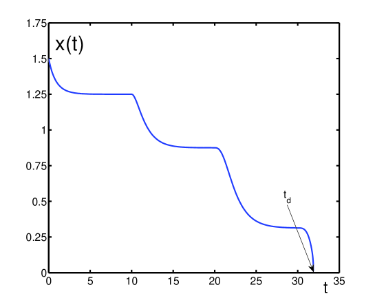
Figure 11: Evolution of the solution to equation (59) for the parameter $b=-1.5<-1$, lag $\tau=10$, with the initial condition $x_{0}=1.5<1/(|b|-1)$. Solution $x(t)$ monotonically decays to finite-time death at $t_{d}\approx 31.884$, defined by (53).

leads to population extinction, at the death time given by Eq. (53). But the dynamics for this case, as is shown in Fig 11, is different from that of Fig. 8. In the present case, there are no alternations, but the decay to zero is monotonic, exhibiting a finite number of quasi-plateaus.

Under the conditions of gain and cooperation, there are two types of extreme events, the finite-time singularity at a critical time $t_{c}$ and the finite-time death at a death time $t_{d}$. The finite-time death is caused by the destructive population activity. And the finite-time singularity means that, close to the singularity point, the system experiences a change of dynamic regime.

6 Society with loss and competition

Under prevailing loss and competition, when

$$\sigma_{1}=-1\;,\qquad\sigma_{2}=1\;,$$ (66)

the evolution equation becomes

$$\frac{dx(t)}{dt}=-x(t)\;-\;\frac{x^{2}(t)}{1+bx(t-\tau)}\;.$$ (67)

There are two stable fixed points. One is the trivial point

$$x_{1}^{*}=0\;,$$ (68)

which is stable for all parameters

$$-\infty<b<\infty\;,\qquad\tau\geq 0\;.$$ (69)

Another stationary point

$$x_{2}^{*}=-\frac{1}{1+b}\equiv x^{*}$$ (70)

is stable for the parameters

$$b<-1\;,\qquad\tau<\tau_{0}\;,$$ (71)

where

$$\tau_{0}\equiv\frac{1}{\sqrt{b^{2}-1}}\;\arccos\left(\frac{1}{|b|}\right)\;.$$ (72)

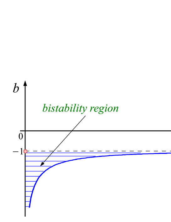
Figure 12: Stability region for the loss-competition case defined in (66).

Thus, there is the bistability region shown in Fig. 12. Solutions tend to one of the two stationary states, when the initial conditions are in the basin of attraction of the corresponding fixed point. The following regimes can arise.

6.1 Monotonic decay to zero

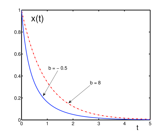
Figure 13: Temporal behavior of the solution to equation (67) for the lag $\tau=10$, initial condition $x_{0}=1$, with the parameters $b=-0.5$ (solid line) and $b=8$ (dashed-dotted line). The initial condition $x_{0}<1/|b|$ for $b<0$. Solutions $x(t)$ monotonically converge to their stationary state $x^{*}=0$.

In a society with prevailing loss and competition, the decay to zero, as in Fig. 13, seems to be a natural type of behavior. This happens when either

$$b>0\;,\qquad\tau\geq 0\qquad(x_{0}>0)\;,$$ (73)

or when

$$b>0\;,\qquad\tau\geq 0\qquad\left(x_{0}<\frac{1}{|b|}\right)\;.$$ (74)

6.2 Oscillatory convergence to stationary state

When the parameters are such that

$$b<-1\;,\qquad 0<\tau<\tau_{0}\qquad\left(x_{0}>\frac{1}{|b|-1}\right)\;,$$ (75)

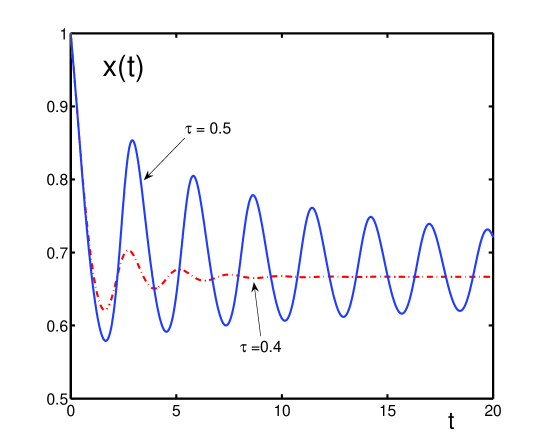
Figure 14: Solutions $x(t)$ to Eq. (67) as functions of time for the parameters $\tau=0.4$ (solid line) and $\tau=0.5$ (dashed-dotted line), where $\tau<\tau_{0}=0.505951$, with $\tau_{0}$ defined by (72). Other parameters are: $x_{0}=1$, and $b=-2.5$. The solutions $x(t)$ converge by oscillating towards their stationary point $x_{2}^{*}=-1/(1+b)=2/3$ as $t\rightarrow\infty$.

the population fraction $x$ oscillates in time, converging to the stationary state (70), as is shown in Fig. 14. Oscillations are caused by the presence of the time delay.

6.3 Everlasting nondecaying oscillations

For the parameters

$$b<-1\;,\qquad\tau_{0}\leq\tau<\tau_{1}\qquad\left(x_{0}>\frac{1}{|b|-1}\right)\;,$$ (76)

the solution oscillates without decay, similarly to the behavior in Fig. 7. The time lag $\tau_{0}$ is given by Eq. (72) and $\tau_{1}$ is defined numerically.

6.4 Punctuated growth to finite-time singularity

A rather interesting behavior of the population dynamics happens for the parameters

$$b<-1\;,\qquad\tau_{1}\leq\tau<\tau_{2}\qquad\left(x_{0}>\frac{1}{|b|-1}\right)\;.$$ (77)

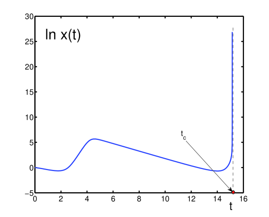
Figure 15: Behavior of the solution $x(t)$ in logarithmic scale to Eq. (67) as a function of time for the parameters $b=-2.5$, $\tau=0.6272$, and the initial history $x_{0}=1$. The solution $x(t)\rightarrow\infty$ as $t\rightarrow t_{c}=15.1498$, where $t_{c}$ is defined by (78).

Then the solution experiences several punctuations, after which it diverges, as is illustrated in Fig. 15, at the critical time defined by the equation

$$1+bx(t_{c}-\tau)=0\;.$$ (78)

When the final rise is preceded by a fall, this behavior is reminiscent of the Parrondo effect [72],

6.5 Up-down convergence to stationary state

A highly non-monotonic behavior exists for the parameters

$$b<-1\;,\qquad 0\leq\tau<\tau_{c}\qquad\left(\frac{1}{|b|}<x_{0}<\frac{1}{|b|-1}\right)\;,$$ (79)

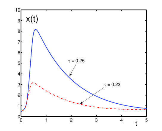
Figure 16: Temporal behavior of solutions $x(t)$ to Eq. (67) as functions of time for the parameters $b=-2.5$ and $\tau=0.25$ (solid line); $\tau=0.23$ (dashed-dotted line); and the initial history $x_{0}=1$. The solution $x(t)\rightarrow x^{*}=2/3$, when $t\rightarrow\infty$.

where the time lag $\tau_{c}$ can be found only numerically. In this case, the solution, first, bursts out upwards, after which it decays to the stationary value $x^{*}$, as in Fig. 16.

6.6 Growth to finite-time singularity

Under the parameters

$$b<-1\;,\qquad\tau>\tau_{c}\qquad\left(\frac{1}{|b|}<x_{0}<\frac{1}{|b|-1}\right)\;,$$ (80)

the solution diverges at a finite critical time, without any punctuation, in the same way as in Fig. 9.

6.7 Unlimited exponential growth

In the region of the parameters

$$-1<b<0\;,\qquad 0<\tau\leq\tau_{c}\qquad\left(x_{0}>\frac{1}{|b|}\right)\;,$$ (81)

the solution grows exponentially, as in Fig. 10.

For a society with prevailing loss and competition, there are two extreme events, both characterized by a finite-time singularity at a critical time $t_{c}$. These regimes occur under a strong destructive activity of the population and a rather long time lag. The divergence can be understood as a critical point where the society dynamics qualitatively changes.

7 Society with loss and cooperation

When loss and cooperation prevail, so that

$$\sigma=-1\;,\qquad\sigma_{2}=-1\;,$$ (82)

the population evolution equation is

$$\frac{dx(t)}{dt}=-x(t)+\frac{x^{2}(t)}{1+bx(t-\tau)}\;.$$ (83)

There exists the sole evolutionary stable state

$$x^{*}=0$$ (84)

that is stable for all parameters

$$-\infty<b<\infty\;,\qquad\tau\geq 0\;.$$ (85)

The following dynamic regimes are possible.

7.1 Monotonic decay to zero

For the initial conditions in the attraction basin of the stable fixed point, the solutions decay to zero with time, as in Fig. 13. This happens when either

$$b<0\;,\qquad\tau\geq 0\qquad\left(x_{0}<\frac{1}{1-b}\right)\;,$$ (86)

or when

$$b>1\;,\qquad\tau\geq 0\qquad\left(x_{0}>\frac{1}{b-1}\right)\;.$$ (87)

7.2 Growth to finite-time singularity

If the initial conditions are outside of the attraction basin of the fixed point (84), they can diverge at a finite critical time, similarly to the behavior in Fig. 9. This happens when either

$$b\leq 0\;,\qquad\tau>0\qquad\left(x_{0}<\frac{1}{|b|}\right)\;,$$ (88)

or when

$$0<b<1\;,\qquad\tau>\tau_{c}\qquad\left(x_{0}>\frac{1}{1-b}\right)\;.$$ (89)

7.3 Unlimited exponential growth

For the parameters

$$0<b<1\;,\qquad\tau<\tau_{c}\qquad\left(x_{0}>\frac{1}{1-b}\right)\;,$$ (90)

the solution exhibits exponential growth, as in Fig. 10.

7.4 Monotonic decay to finite-time death

Finally, for the parameters

$$b<0\;,\qquad 0\leq\tau<\tau_{d}\qquad\left(x_{0}>\frac{1}{|b|}\right)\;,$$ (91)

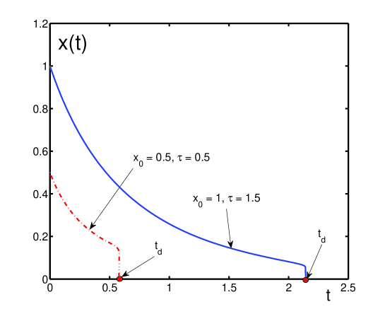
Figure 17: Behavior of solutions $x(t)$ to Eq. (83) as functions of time for $b=-2.5$, lag $\tau=1.5$, history $x_{0}=1$ (solid line), and lag $\tau=0.5$, history $x_{0}=0.5$ (dashed-dotted line). At the moment $t=t_{d}$, defined as $1+bx(t_{d}-\tau)=0$, solutions monotonically decay to zero, $x(t_{d})=0$, $\dot{x}(t)|_{t=t_{d}}=-\infty$. The death time for the population, represented by the solid line, is $t_{d}=2.14158$, and the death time for the population shown by the dashed-dotted line, is $t_{d}=0.58004$.

the population becomes extinct at a finite death time, as in Fig. 17. The death time is defined by an equation having the same form as Eq. (53). However the decay to death now is monotonic, which distinguishes it from the punctuated behavior before death, shown in Fig. 8 and Fig. 11.

The society with prevailing loss and cooperation can exhibit the finite-time singularity as well as the finite-time death. These two types of extreme events happen under the destructive activity of population.

Summarizing, all extreme events, except one, occur when the population destroys its carrying capacity. The sole exception is the case of a society with gain and cooperation, when there can arise a finite-time singularity under $b>0$, i.e., when the activity of the population is productive. This latter type of finite-time singularity is analogous to that studied in Ref. [27]. Its appearance means that, near the critical time, the society becomes unstable and requires to change its parameters, for instance replacing cooperation by competition. It seems to be rather clear that, when the population grows too much, the competition of individuals must come into play, becoming prevailing over their cooperation. The finite-time singularities, occurring under the destructive society activity, imply the existence of some critical events, whose detailed interpretation will be given in Sec. 11.

8 Mutual influence of symbiotic species on their carrying capacities

8.1 Classification of symbiosis types

When the considered society is structured with several species, it is necessary to characterize their interactions. The standard way of doing this is by assuming the equations of the predator-prey type (3), with direct interactions of species that eat each other. Such equations, however, cannot describe indirect interactions, when the species do not kill each other, but influence the carrying capacities of each other. Therefore, the predator-prey equations are suitable for describing the predator-prey relations, but are not suitable for characterizing symbiotic relations [40].

Examples of symbiosis are ubiquitous in biology and ecology [73, 74, 75, 76]. It is also widespread in human societies. For example, one can treat as symbiotic the interrelations between firms and banks, between population and government, between culture and language, between economics and arts, and between basic science and applied research.

Considering purely symbiotic relations, we need equation (14), with the carrying capacities being functionals of the species populations. The natural form of such carrying capacities for symbiotic species is

$$K_{i}=A_{i}+B_{i}S_{i}(\{N_{i}\})\;.$$ (92)

Here $A_{i}>0$ is the natural carrying capacity, provided by nature, for an $i$-th species. The coefficient $B_{i}$ characterizes the strength of influence of other species on the carrying capacity of the $i$-th species. When $B_{i}$ is positive, it can be called the production factor, while, if it is negative, it is the destruction factor. The function $S(\{N_{i}\})$ is a symbiotic function specifying the mutual relations between symbiotic species. Since the sign has already been attributed to the factor $B_{i}$, the symbiotic function can be treated as non-negative.

Depending on the kinds of symbiotic relations, that is, on the signs of the factors $B_{i}$, there can occur different variants of symbiosis. To illustrate this, let us analyze the case of two symbiotic species for which there can exist the following types of symbiosis.

(i) Mutualism, when both species are useful for each other, developing their mutual carrying capacities:

$$B_{1}>0\;,\qquad B_{2}>0\quad(mutualism)\;.$$ (93)

(ii) Parasitism, when one of the species is harmful for another, or both species are harmful for each other, destroying the carrying capacities, which happens under one of the pairs of inequalities below:

$$\begin{array}[]{lll}B_{1}>0\;,&\qquad B_{2}<0\;,&\\ B_{1}<0\;,&\qquad B_{2}>0\;,&\quad(parasitism)\\ B_{1}<0\;,&\qquad B_{2}<0~{}.&\end{array}$$ (97)

(iii) Commensalism, when one of the species is useful for another, while the latter is indifferent to the existence of the first species, which corresponds to the validity of one of the pairs of equations:

$$\begin{array}[]{lll}B_{1}>0\;,&\qquad B_{2}=0\;,&\\ B_{1}=0\;,&\qquad B_{2}>0&\quad(commensalism)\;.\end{array}$$ (100)

8.2 Normalized species fractions

We continue analyzing the symbiotic coexistence of two kinds of species. As always, it is more convenient to work with reduced quantities. So, we introduce the reduced fractions

$$x\equiv\frac{N_{1}}{N_{eff}}\;,\qquad z\equiv\frac{N_{2}}{Z_{eff}}\;,$$ (101)

whose normalization values $N_{eff}$ and $Z_{eff}$ will be chosen later. We define the dimensionless carrying capacities

$$y_{1}\equiv\frac{\gamma_{1}K_{1}}{C_{1}N_{eff}}\;,\qquad y_{2}\equiv\frac{\gamma_{1}K_{2}}{C_{2}Z_{eff}}$$ (102)

and the relative birth rate

$$\alpha\equiv\frac{\gamma_{2}}{\gamma_{1}}\;.$$ (103)

With these notations, the symbiotic equations (14), in the case of two types of species, reduce to

$$\frac{dx}{dt}=x\;-\;\frac{x^{2}}{y_{1}}\;,\qquad\frac{dz}{dt}=\alpha z\;-\;\frac{z^{2}}{y_{2}}\;,$$ (104)

where time is measured in units of $1/\gamma_{1}$. By their definition, the solutions $x$ and $y$ are non-negative. The equations are complemented by the initial conditions

$$x(0)=x_{0}\;,\qquad z(0)=z_{0}\;.$$ (105)

For the following analysis, it is necessary to make concrete the explicit forms of the carrying capacities (92).

9 Symbiosis with mutual interactions

9.1 Derivation of normalized equations

The action of the species on the carrying capacities of each other can be different, depending on whether, influencing the carrying capacities, the species interact or not. If the species, in the process of influencing their carrying capacities, interact with each other, then the carrying capacities (92) can be represented in the form

$$K_{1}=A_{1}+B_{1}N_{1}N_{2}\;,\qquad K_{2}=A_{2}+B_{2}N_{2}N_{1}\;.$$ (106)

Generally, the populations $N_{1}$ and $N_{2}$ in these carrying capacities could depend on the shifted time, when one would have

$$K_{i}=A_{i}+B_{i}N_{i}(t-\tau_{i})N_{j}(t-\tau_{j})\;,$$

where $i\neq j$. However, we need, first, to understand the influence of symbiosis without the time lag. Therefore, we consider below the interactions without time delay.

Introducing the dimensionless natural carrying capacities

$$a_{1}\equiv\frac{\gamma_{1}A_{1}}{C_{1}N_{eff}}\;,\qquad a_{2}\equiv\frac{\gamma_{1}A_{2}}{C_{2}Z_{eff}}\;$$ (107)

and dimensionless symbiotic factors

$$b\equiv\frac{\gamma_{1}B_{1}Z_{eff}}{C_{1}}\;,\qquad g\equiv\frac{\gamma_{1}B_{2}N_{eff}}{C_{2}}$$ (108)

translates Eqs. (106) into the dimensionless expressions

$$y_{1}=a_{1}+bxz\;,\qquad y_{2}=a_{2}+gxz\;.$$ (109)

Since the scaling values $N_{eff}$ and $Z_{eff}$ are arbitrary, it is reasonable to choose them so as to simplify the equations. For this purpose, we set

$$N_{eff}\equiv\frac{\gamma_{1}A_{1}}{C_{1}}\;,\qquad Z_{eff}\equiv\frac{\gamma_{1}A_{2}}{C_{2}}\;.$$ (110)

Then the natural carrying capacities (107) become

$$a_{1}=a_{2}=1\;.$$ (111)

And the total carrying capacities (109) read as

$$y_{1}=1+bxz\;,\qquad y_{2}=1+gxz\;.$$ (112)

As usual, we measure time in units of $1/\gamma_{1}$. The most interesting case in symbiosis is when the species influence each other throughout their lifetimes, and when these lifetimes are of comparable durations. If this were not the case, i.e., with very different lifetimes, the symbiotic relations could not be supported for a duration longer than the shortest lifespan, making symbiosis inefficient for the longer-lived species. Therefore, we assume that the symbiotic species have comparable growth rates, because the inverse of the growth rate sets the time scale of lifetime, and the later is often found proportional to the growth period, at least for mammals [77]. We thus set $\alpha=1$ and obtain the equations

$$\frac{dx}{dt}=x\;-\;\frac{x^{2}}{1+bxz}\;,\qquad\frac{dz}{dt}=z\;-\;\frac{z^{2}}{1+gxz}\;.$$ (113)

We can note that these equations are symmetric with respect to the simultaneous interchange between $x$ with $z$ and between $b$ with $g$. This symmetry will result in the corresponding symmetry of the following solutions.

9.2 Evolutionary stable states

Again we use the Lyapunov stability analysis [11, 16, 70]. Equations (113) possess the non-zero stationary state

$$x^{*}=\frac{1}{2g}\left[1-b+g-\sqrt{(1+b-g)^{2}-4b}\right]\;,$$

$$z^{*}=\frac{1}{2b}\left[1+b-g-\sqrt{(1+b-g)^{2}-4b}\right]\;.$$ (114)

It is stable when either

$$b<0\;,\qquad-\infty<g<+\infty\;,$$ (115)

or when

$$0\leq b<1\;,\qquad g\leq g_{c}\;,$$ (116)

or when

$$b\geq 1\;,\qquad g\leq 0\;,$$ (117)

where the critical value $g_{c}$ is

$$g_{c}\equiv\left(1-\sqrt{b}\right)^{2}\leq 1\;.$$ (118)

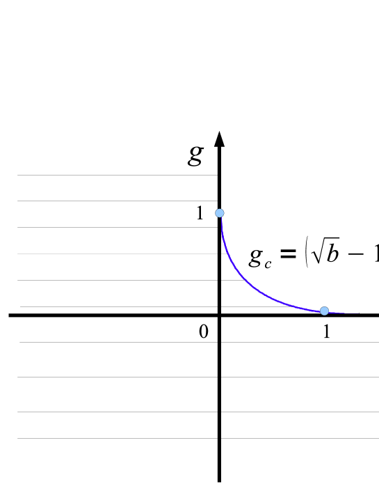
Figure 18: Region of stability (shaded) in the parameter plane $b-g$ for the stationary solutions in the case of symbiosis with mutual interactions.

The stability region is depicted in Fig. 18. The basin of attraction of this stationary state, depending on the signs of the symbiotic factors, is defined by the following equations:

$$x_{0}z_{0}<\frac{1}{|b|}\qquad(b<0,\;g>0)\;,$$

$$x_{0}z_{0}<\frac{1}{|g|}\qquad(b>0,\;g<0)\;,$$

$$x_{0}z_{0}<min\left\{\frac{1}{|b|}\;,\frac{1}{|g|}\right\}\qquad(b<0,\;g<0)\;.$$ (119)

The solutions to the symbiotic equations (113) should be compared to those of the uncoupled equations

$$\frac{dx}{dt}=x-x^{2}\;,\qquad\frac{dz}{dt}=z-z^{2}\qquad(b=g=0)\;,$$ (120)

corresponding to the case of no symbiosis, when the stationary states are $x^{*}=z^{*}=1$.

Solving numerically the system of equations (113) for different symbiotic factors and initial conditions yields the following possible dynamic regimes.

9.3 Convergence to stationary states

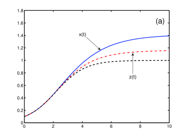
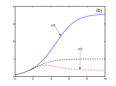
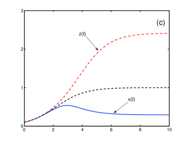
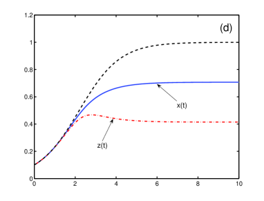
Figure 19: Comparison of the symbiotic solutions $x(t)$ (solid line) and $z(t)$ (dashed-dotted line), for the symbiosis with mutual interactions (113), with the solutions $x(t)=z(t)$ (dashed line) of the decoupled equations (120) for the same initial conditions $x_{0}=z_{0}=0.1<1$, with different symbiotic parameters $b$ and $g$: (a) $b=0.25$, $g=0.1<g_{c}=0.25$, the stationary points of the symbiotic equations being $x^{*}=1.411$, $z^{*}=1.164$; (b) $b=2$, $g=-0.5$, the fixed points of the symbiotic equations being $x^{*}=3.562$, $z^{*}=0.360$; (c) $b=-1$, $g=2$, the symbiotic fixed points being $x^{*}=0.293$, $z^{*}=2.414$; (d) $b=-1$, $g=-2$, the symbiotic fixed points being $x^{*}=0.707$, $z^{*}=0.414$.

For the system parameters in the region of stability and for the initial conditions in the basin of attraction of the non-zero fixed point (114), both species develop and converge to the stationary state. This is illustrated in Fig. 19 for different types of symbiosis, where, for comparison, the solutions for the case of no symbiosis are also presented. The four possible cases are illustrated in the four panels of Fig. 19, depending on the relative positions of $x(t)$ and $z(t)$ compared with the solution of the uncoupled equations (120).

9.4 Unlimited exponential growth

When stationary solutions do not exist, so that either

$$0<b<1\;,\qquad g>g_{c}\;,$$ (121)

or when

$$b>1\;,\qquad g>0\;,$$ (122)

or when they exist, but the initial conditions are taken outside of the attraction basin, then the populations of both species grow exponentially with time.

9.5 Finite-time death and singularity

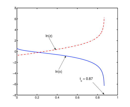
Figure 20: Behavior of the solutions in logarithmic scale to equations (113) in the case of finite-time death and singularity, $x(t)$ (solid line) and $z(t)$ (dashed-dotted line), for the parasitic relations with the symbiotic coefficients $b=-1$, $g=-2$, under the initial conditions $x_{0}=1.8$, $z_{0}=0.5$. For these parameters, the critical time is $t_{c}=0.87$.

In the case of mutual parasitism, there can happen an extreme solution when one of the species becomes extinct at a finite critical time, while the other species displays a finite-time singularity, as is shown in Fig. 20. This happens when the initial conditions are outside of the attraction basin so that either

$$\frac{1}{|b|}<x_{0}z_{0}<\frac{1}{|g|}\qquad(b<g<0)\;,$$ (123)

or if

$$\frac{1}{|g|}<x_{0}z_{0}<\frac{1}{|b|}\qquad(g<b<0)\;.$$ (124)

The critical time is defined by one of the corresponding equations:

$$x(t_{c})z(t_{c})=\frac{1}{|b|}\qquad(b<g<0)\;,$$

$$x(t_{c})z(t_{c})=\frac{1}{|g|}\qquad(g<b<0)\;.$$ (125)

The appearance of such an extreme solution is caused by the mutual parasitism of the species, destroying the carrying capacities of each other.

10 Symbiosis without direct interactions

10.1 Derivation of symbiotic equations

In many cases, symbiotic species influence each other by increasing (improving) the carrying capacities of each other, which does not involve direct interactions between the species. The most known example of this type is the symbiosis between tree roots and fungi. In that case, the carrying capacities (92) can be written in the form

$$K_{1}=A_{1}+B_{1}N_{2}\;,\qquad K_{2}=A_{2}+B_{2}N_{1}\;.$$ (126)

The dimensionless carrying capacities (102) now read as

$$y_{1}=a_{1}+bz\;,\qquad y_{2}=a_{2}+gx\;.$$ (127)

Employing the scaling of Eqs. (110) gives normalization (111) and the carrying capacities (127) become

$$y_{1}=1+bz\;,\qquad y_{2}=1+gx\;.$$ (128)

Thus, we come to the symbiotic equations in dimensionless form

$$\frac{dx}{dt}=x\;-\;\frac{x^{2}}{1+bz}\;,\qquad\frac{dz}{dt}=z\;-\;\frac{z^{2}}{1+gx}\;.$$ (129)

There exists again the symmetry with respect to the simultaneous interchange between $x$ and $z$ and between $b$ and $g$.

10.2 Evolutionary stable states

Equations (129) possess a non-zero stationary state

$$x^{*}=\frac{1+b}{1-bg}\;,\qquad z^{*}=\frac{1+g}{1-bg}\;,$$ (130)

which is stable when either

$$-1\leq b<0\;,\qquad g\geq-1\;,$$ (131)

or when

$$b\geq 0\;,\qquad 0\leq g\leq g_{c}\;,$$ (132)

where

$$g_{c}\equiv\frac{1}{b}\;.$$ (133)

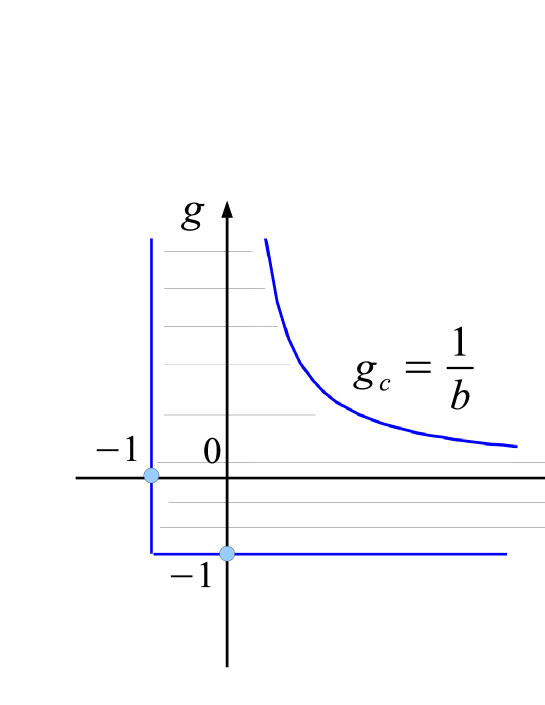
Figure 21: Region of stability (shaded) in the parameter plane $b-g$ for the fixed points in the case of symbiosis without direct interactions.

The stability region is presented in Fig. 21.

If the symbiotic relations correspond to mutualism or commensalism, then the attraction basin of the stationary solution (130) is the whole region of positive initial conditions:

$$x_{0}>0\;,\qquad z_{0}>0\qquad(b\geq 0,\;0\leq g<g_{c})\;.$$ (134)

But if at least one of the species is parasitic, then the attraction basins are defined by one of the conditions, depending on the signs of the symbiotic factors:

$$x_{0}<\frac{1}{|g|}\;,\qquad z_{0}>0\qquad(b>0,\;g<0)\;,$$

$$x_{0}>0\;,\qquad z_{0}<\frac{1}{|b|}\qquad(b<0,\;g>0)\;,$$

$$x_{0}<\frac{1}{|g|}\;,\qquad z_{0}<\frac{1}{|b|}\qquad(b<0,\;g<0)\;.$$ (135)

The following dynamic regimes are possible.

10.3 Convergence to stationary states

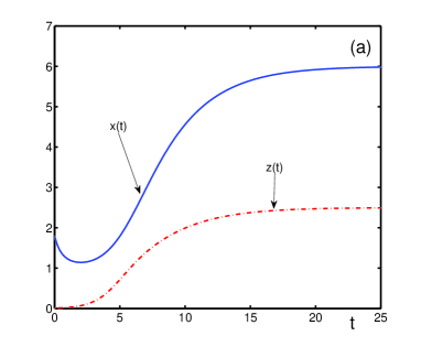
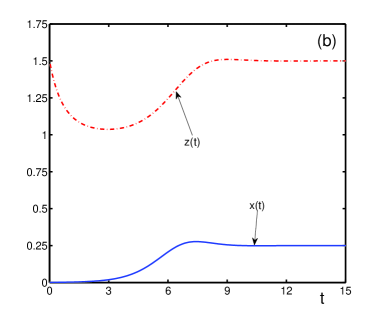
Figure 22: Nonmonotonic convergence to stationary states of $x(t)$ (solid line) and $z(t)$ (dashed-dotted line) as functions of time, in the case of symbiosis without direct interactions (129): (a) for the initial conditions $x_{0}=1.8$, $z_{0}=0.01$ and the parameters $b=2$, $g=0.25$. The functions $x(t)\rightarrow x^{*}$ and $z(t)\rightarrow z^{*}$, when $t\rightarrow\infty$, the fixed points being $x^{*}=6$, $z^{*}=2.5$; (b) for the initial conditions $x_{0}=0.001$, $z_{0}=1.5$, and the parameters $b=-0.5$, $g=2$. Functions $x(t)\rightarrow x^{*}=0.25$ and $z(t)\rightarrow z^{*}=1.5$, when $t\rightarrow\infty$.

If initial conditions are in the attraction basin, then both species converge to their stationary populations. The convergence can be monotonic or not, depending on the system parameters and initial conditions, as is demonstrated in Fig. 22.

10.4 Unlimited exponential growth

For the parameters outside the stability region, such that

$$b>0\;,\qquad g>g_{c}\;,$$ (136)

there exists a solution with exponential growth in time for both species.

10.5 Finite-time divergence

Extreme solutions appear when at least one of the species is parasitic and initial conditions are outside of the attraction basin. Thus, when either

$$x_{0}>\frac{1}{|g|}\;,\qquad z_{0}>0\qquad(b>0,\;g<0)\;,$$ (137)

or when

$$x_{0}>0\;,\qquad z_{0}>\frac{1}{|b|}\qquad(b<0,\;g>0)\;,$$ (138)

then one of the species experiences a finite-time singularity at a critical time $t_{c}$ that is defined numerically. In this case, when approaching $t_{c}$, one of the following behaviors arise:

$$x(t)\rightarrow x(t_{c})<\infty\;,\qquad z(t)\rightarrow\infty\;,$$

$$x(t)\rightarrow\infty\;,\qquad z(t)\rightarrow z(t_{c})<\infty\;,$$ (139)

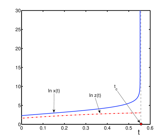
Figure 23: Behavior of the solutions $x(t)$ (solid line) and $z(t)$ (dashed-dotted line) in logarithmic scales in the case of symbiosis without direct interactions (129) in the presence of the finite-time singularity for the symbiotic coefficients $b=-0.75$, $g=-0.25$, and the initial conditions $x_{0}=10$, $z_{0}=5$. The critical time is $t_{c}=0.55303$.

where the first line corresponds to conditions (137), while the second line, to conditions (138). The typical behavior of populations is shown in Fig. 23.

10.6 Finite-time extinction

Parasitic symbiotic relations may end with one of the species being extinct and the other continuing its life without symbiosis. When either

$$x_{0}<\frac{1}{|g|}\;,\qquad z_{0}>0\qquad(b>0,\;g\leq-1)\;,$$ (140)

or when

$$x_{0}<\frac{1}{|g|}\;,\qquad z_{0}>\frac{1}{|b|}\qquad(b<0,\;g<0)\;,$$ (141)

then the species $z$ dies at a finite time $t_{d}$, defined by the relation

$$x(t_{d})=\frac{1}{|g|}\;.$$ (142)

That is, the species $x$ kills the species $z$:

$$x(t)\rightarrow x(t_{d})\;,\qquad z(t)\rightarrow 0\qquad(t\rightarrow t_{d})\;.$$ (143)

The opposite situation, when the species $z$ kills the species $x$ occurs if either

$$x_{0}>0\;,\qquad z_{0}<\frac{1}{|b|}\qquad(b\leq-1,\;g>0)\;,$$ (144)

or if

$$x_{0}>\frac{1}{|g|}\;,\qquad z_{0}<\frac{1}{|b|}\qquad(b<0,\;g<0)\;.$$ (145)

Then the species $x$ dies at a finite time given by the relation

$$z(t_{d})=\frac{1}{|b|}\;,$$ (146)

so that

$$x(t)\rightarrow 0\;,\qquad z(t)\rightarrow z(t_{d})\qquad(t\rightarrow t_{d})\;.$$ (147)

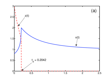
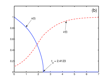
Figure 24: Finite-time death in the case of symbiosis without direct interactions. Temporal behavior of solutions $x(t)$ (solid line) and $z(t)$ (dashed-dotted line) for different symbiotic parameters and initial conditions: (a) $b=-0.75$, $g=-0.5$, $x_{0}=0.8$, $z_{0}=3$, the death time being $t_{d}=0.204$; (b) $b=-1.5$, $g=1$, $x_{0}=1$, $z_{0}=0.1$, with the death time $t_{d}=2.412$.

The corresponding behavior is illustrated in Fig. 24.

11 Interpretation of extreme events in population evolution

11.1 Types of extreme events

In the population evolution, there may happen two types of extreme events, finite-time death and finite-time singularity. The origin for the occurrence of finite-time death is rather clear. This happens when the carrying capacity of the species is destroyed, either by the species themselves or by the parasitic symbiosis of other species. The destroyed carrying capacity makes it impossible the long-term existence of the species that, thus, go towards extinction.

Finite-time singularity can be due to two causes. One reason is the existence of cooperation between the members of species, as in Secs. 5.1 and 7.2. This type of the finite-time singularity means that the society, in which cooperation persists under fast increasing numbers of its members, becomes unstable and, to be stabilized, requires that cooperation be changed into competition. The necessity for such a change looks rather evident and is easily understandable. Really, in the presence of a strongly increasing population, the competition for the means of survival will become unavoidable.

A more elaborate mechanism operates in the case of the finite-time singularities occurring under competition, as in Secs. 4.8, 6.4, 6.6, 9.5, and 10.5. In all these cases, the singularities appear under the destruction of the carrying capacities either by the society itself or by a parasitic symbiotic species. It may seem quite strange that, while the carrying capacity is being destroyed, the population continues growing. To understand the origin of such a paradoxical effect and of these finite-time singularities, let us consider in turn the different types of finite-time singularities found in Secs. 4.8, 6.4, 6.6, 9.5, and 10.5.

11.2 Boom and crash in society with gain and competition

This corresponds to the case studied in Sec. 4.8, of a finite-time singularity occurring at a critical time $t_{c}$. The divergence is of the hyperbolic type (56). This extreme event happens under the destructive action of the society on its own carrying capacity, when $b<0$. The parameters are such that, at the initial moment of time, the effective carrying capacity is negative,

$$y(0)=1-|b|x_{0}<0\;.$$ (148)

How would it be possible to understand the existence of a negative carrying capacity? For some simple biological species, as ants or bees, the negative capacity would, probably, be impossible. Such species would not be able to live at all. However, for more complex societies such as human societies, the negative carrying capacity may have sense. For instance, humans do extract non-renewable resources that become progressively exhausted forever, they destroy their habitat, poison rivers, pollute air, cut forests, and so on. At the same time, humans possess the ability of regenerating the habitat by cleaning rivers, or even oceans, and planting trees. Thus, humans may spoil their habitat to such an extent that it would require a hard work for its recovering. In that sense the effective carrying capacity can become negative for a while, implying the necessity of its recuperation in the positive domain in order to ensure the long-term survival of the human society [78].

Even more transparent is the explanation for the existence of negative carrying capacity for financial and economic societies, when the variable $x$ represents not population, but capitalization. In these cases, negative capacity is nothing but the borrowed resources that have to be returned back to the lender. Due to this leverage effect resulting from borrowing, a firm can exhibit a fast development. But borrowing cannot last forever. If the firm, society, or country does not produce enough and is not able to pay debts, its creditors will lose trust and may require early reimbursement, or will simply refuse rolling over the debts, as occurred for Greece in May 2010 and Ireland in November 2010. This situation can be captured by assuming the existence of a maximum level of debt, beyond which the society or country becomes highly unstable due to feedbacks resulting from market forces. Actually, Reinhart and Rogoff [79] have recently documented the existence of a strong link between levels of debt and countries’ economic growth over the last two centuries: Countries with a gross public debt exceeding about 90% of annual economic output tended to grow a lot more slowly and to exhibit larger default risks.

Assuming the existence of a maximum debt level beyond which instabilities appear leads to the existence of a time $t_{crash}$ beyond which a crash or at least strong turbulence can occur. This is highly reminiscent of the scenario leading to the “great recession” that started in 2007 worldwide [80]. The minimum crash time $t_{crash}$ is thus given by the condition that the debt, represented by the negative carrying capacity, reaches the value

$$y(t_{crash})=1-|b|x(t_{crash}-\tau)<0\;.$$ (149)

The crash happens before the critical divergence time $t_{c}$,

$$t_{crash}<t_{c}\;,$$ (150)

where the firm or country capitalization is still finite. In such a regime, the accelerated growth, fueled by borrowing, leads to a boom that is not supported by increasing productivity. This can therefore be called a bubble [28]. As the bubble develops, it eventually reaches a threshold level beyond which it becomes unstable, and can therefore be followed by a crash at times between $t_{crash}$ and $t_{c}$.

11.3 Boom and crash in society with loss and competition

The same interpretation as above is applicable for the society with loss and competition, as in Secs. 6.4 and 6.6. There, the finite-time singularity arises under a high level of destruction, when the destruction coefficient $b<-1$ and the initial carrying capacity is negative. The hyperbolic divergence occurs at a critical time $t_{c}$. In Sec. 6.6, the situation is similar to that discussed above. The difference between Sec. 6.4 and Sec. 6.6 is that in Sec. 6.4 the divergence is defined by the equation

$$y(t_{c})=1-|b|x(t_{c}-\tau)=0\;.$$ (151)

Again, a society or a firm with loss and competition, actually, does not reach the point of divergence, but becomes bankrupt before this. The fast growth is due to exploiting and destroying the carrying capacity. But, after destruction has taken place and reached an unbearable level, the boom is followed by a crash.

11.4 Species extinction under mutual parasitic symbiosis

In the parasitic symbiosis of two species considered in Sec. 9.5, there occurs a finite-time singularity. Thus, for the symbiotic parameters $b<g<0$, the initial carrying capacities are such that

$$y_{1}(0)=1-|b|x_{0}z_{0}<0\;,\qquad y_{2}(0)=1-|g|x_{0}z_{0}>0\;.$$ (152)

For the opposite case, when $g<b<0$, the situation is symmetric. Thence, below we shall treat the case of Eq. (152) without loss of generality. The divergence appears at the critical time $t_{c}$ given by the equation

$$y_{1}(t_{c})=1-|b|x(t_{c})z(t_{c})\;.$$ (153)

At this time, the population of the species $x$ tends to infinity, while that of the species $z$ goes to zero.

Of course, no realistic population can rise to infinite values. Such a divergence happens because of the mutual parasitic symbiotic relations, resulting in the formal appearance of a negative effective capacity. As in the cases above, the divergence can be avoided by limiting the carrying capacity by a fixed level. This implies that the rise of a parasitic species continues only up to some limiting carrying capacity threshold

$$y_{1}(t_{crash})=1-|b|x(t_{crash})z(t_{crash})\;,$$ (154)

after which the species $x$ dies out by a fast process of extinction at the crash time $t_{crash}<t_{c}$.

11.5 Species extinction under parasitic symbiosis without direct interactions

A finite-time singularity also appears in the case of symbiosis without direct interactions, as in Sec. 10.5. This happens when at least one of the species is parasitic. For example, for the case $b<0$ and $b<g$. Below, we shall consider this case, since the situation with $g<0$ and $g<b$ is symmetric.

When $b<0$, this means that the species $z$ is parasitic and destroys the carrying capacity of the species $x$. The finite-time singularity occurs if, at the initial moment of time, the effective carrying capacity of species $x$ is negative,

$$y_{1}(0)=1-|b|z_{0}<0\;,$$ (155)

while the carrying capacity of species $z$,

$$y_{2}(0)=1+gx_{0}\;,$$ (156)

can be positive or negative, depending on the values of $g$ and $x_{0}$. The divergence of $x$ occurs at the critical time $t_{c}$, where the effective capacity of species $x$ is negative,

$$y_{1}(t_{c})=1-|b|z(t_{c})<0\;.$$ (157)

The population of species $z$ at the moment $t_{c}$ is finite.

In the same way as in the previous cases, we understand that this divergence cannot be real and there should exist a limiting carrying capacity

$$y_{1}(t_{crash})=1-|b|z(t_{crash})\;,$$ (158)

at which the population $x$ is to be set to zero, implying its extinction caused by the parasitic species $z$. This extinction happens at the crash time $t_{crash}<t_{c}$.

In all these cases for which there arises a finite-time singularity, it is possible to exclude the formal divergence by limiting the carrying capacity to a minimal value $y(t_{crash})$, that is, a maximal absolute value $|y(t_{crash})|$. This limiting value can be interpreted as a threshold for a change of regime. The overall dynamics, thus, starting with the fast growth of the population (or capitalization), is followed by its drop to zero at the crash time $t_{crash}$, before the critical time $t_{c}$.

12 Conclusion

In this paper, we have suggested a general approach for describing the evolution of populations, whose activities influence their carrying capacities. In order to take into account this influence, the carrying capacities are to be defined as functions of the society populations. This includes the action of a population on its own carrying capacity. In general, the actions of populations on the carrying capacities can be delayed, since such actions, generally, require time for their realization.

The approach is illustrated by analyzing the time evolution of a society that acts on its own carrying capacity, either by producing the increase of the capacity or by destroying it. Different types of societies have been studied, depending on the balance between gain and loss and between competition and cooperation. A detailed classification of admissible dynamic regimes has been given.

Two kinds of extreme events have been found to arise, when the society destroys its carrying capacity. One is a finite-time death at a death time $t_{d}$ and another is a finite-time singularity at a critical time $t_{c}$. The finite-time death describes the extinction of the population because of the destruction of the carrying capacity. The finite-time singularity signals that the society becomes unstable and its stabilization requires changing the society parameters and a transfer to another dynamic regime. The divergence can be avoided by limiting the carrying capacity and interpreting the effect as a fast rise of the population (or capitalization), followed by its sharp drop. For economic and financial societies, the fast growth is understood as a boom or bubble, due to the leverage effect induced by over-indebtedness, after which a crash occurs.

The suggested approach is also illustrated by considering the symbiosis of several species. This approach allows us to give a general classification of different symbiosis types. The case of two species is analyzed in detail. Extreme events arise when at least one of the species is parasitic, destroying the carrying capacity of the other species. Again, there can exist two kinds of such extreme events, finite-time death and finite-time singularity. Their interpretation is analogous to that given for the case of the self-destructing population activity.

As a general conclusion valid for the different considered situations, we have to say that any destructive action of populations, whether on their own carrying capacity or on the carrying capacities of co-existing species, can lead to the instability of the society that is revealed in the form of the appearance of extreme events, finite-time extinctions or booms followed by crashes.

Acknowledgement: We acknowledge financial support from the ETH Competence Center “Coping with Crises in Complex Socio-Economic Systems” (CCSS) through ETH Research Grant CH1-01-08-2 and ETH Zurich Foundation.

Figure 5: Temporal behavior of solutions to equation (42) for the lag $\tau=20$, parameters $b=-1/3$, $x_{0}=1.5$ (solid line), and $b=-2/3$, $x_{0}=0.1$ (dashed-dotted line). Solutions $x(t)\rightarrow x^{*}$, oscillating by steps, when $t\rightarrow\infty$. The stationary points are $x^{*}=0.75$ and $x^{*}=0.6$, respectively.

Figure 6: Temporal behavior of the solution to equation (42) for the parameter $b=-2<-1$, lag $\tau=1.18<\tau_{0}$, where $\tau_{0}=1.2092$ is defined by (46), with the initial condition $x_{0}=0.25<1/|x_{0}|$. Solution $x(t)\rightarrow x^{*}=1/3$, oscillating, when $t\rightarrow\infty$.

Figure 7: Dynamics of the solution to equation (42) for the parameter $b=-2<-1$, lag $\tau_{0}<\tau=1.5<\tau_{1}$, where $\tau_{0}=1.2092$ is defined by (46), $\tau_{1}=\tau_{1}(b)\approx 1.65$, with the initial condition $x_{0}=0.25<1/|b|$. Solution $x(t)$ oscillates without convergence, when $t\rightarrow\infty$.

Figure 8: Dynamics of the solution to equation (42) for the parameter $b=-2<-1$, lag $\tau=1.7>\tau_{1}$, where $\tau_{1}\approx 1.65$ is defined numerically, with the initial condition $x_{0}=0.25<1/|b|$. Solution $x(t)$ exists only till the moment $t=t_{d}\approx 19.975$, defined by (53).

References

- [1] A.J. Lotka, Elements of Physical Biology (Williams and Wilkins, Baltimore, 1925).
- [2] V. Volterra, Nature 118, 558 (1926).
- [3] H.I. Freedman, Deterministic Mathematical Models in Population Ecology (Marcel Dekker, New York, 1980).
- [4] F. Brauer, C. Castillo-Chavez, Mathematical Models in Population Biology and Epidemiology (Springer, Heidelberg, 2000).
- [5] J. Hofbauer, K. Sigmund, The Theory of Evolution and Dynamical Systems (Cambridge University, Cambridge, 1988).
- [6] S. Smale, J. Math. Biol. 3, 5 (1976).
- [7] M. Hirsch, SIAM J. Math. Anal. 16, 423 (1985).
- [8] M. Hirsch, Nonlinearity 1, 51 (1988).
- [9] M. Hirsch, SIAM J. Math. Anal. 21, 1225 (1990).
- [10] R. Cressman, Evolutionary Dynamics and Extensive Form Games ( Massachusetts Institute of Technology, Cambridge, 2003).
- [11] R.M. May, Stability and Complexity in Model Ecosystems (Princeton University, Princeton, 1974).
- [12] C.S. Holling, C.S., 1959. Canad. Entomol. 91, 293 (1959).
- [13] P.F. Verhulst, Corr. Math. Phys. 10, 113 (1838).
- [14] G.E. Hutchinson, Ann. N.Y. Acad. Sci. 50, 221 (1948).
- [15] K. Gopalsamy, Stability and Oscillations in Delay Differential Equations of Population Dynamics (Kluwer, Dordrecht, 1992).
- [16] V. Kolmanovskii, A. Myshkis, Introduction to the Theory and Applications of Functional Differential Equations (Kluwer, Dordrecht, 1999).
- [17] J. Arino, L. Wang, G.L. Wolkowicz, J. Theor. Biol. 241, 109 (2006).
- [18] M. Peschel, W. Mende, The Predator-Prey Model. Do We Leave in a Volterra World? (Springer, Wien, 1986).
- [19] H. Haberl, H.P. Aubauer, J. Theor. Biol. 156, 499 (1992).
- [20] T.R. Malthus, An Essay on the Principle of Population (John Murray, London, 1826).
- [21] H. von Foerster, P.M. Mora, L.W. Amiot, Science 132, 1291 (1960).
- [22] S.A. Umpleby, Popul. Environm. 11, 159 (1990).
- [23] S.P. Kapitza, Phys. Usp. 166, 63 (1996).
- [24] S.D. Varfolomeev, K.G. Gurevich, J. Theor. Biol. 212, 367 (2001).
- [25] A.V. Markov, A.V. Korotayev, Palaeoworld 16, 311 (2007).
- [26] M. Kremer, Quarter. J. Econom. 108, 681 (1993).
- [27] A. Johansen, D. Sornette, Physica A 294, 465 (2001).
- [28] D. Sornette, Why Stock Markets Crash. Critical Events in Complex Financial Systems (Princeton University, New Jersey, 2003).
- [29] S. Sammis, D. Sornette, Proc. Natl. Acad. Sci. USA 99, 2501 (2002).
- [30] V.I. Yukalov, A. Moura, H. Nechad, J. Mech. Phys. Solids 52, 453 (2004).
- [31] V. Dakos, M. Scheffer, E. van Nes, V. Brovkin, V. Petoukhov, H. Held, Proc. Natl. Acad. Sci. USA 105, 14308 (2008).
- [32] M. Scheffer, J. Bascompte, W.A. Brock, V. Brovkin, S.R. Carpenter, V. Dakos, H. Held, E.H. van Nes, M. Rietkerk, G. Sugihara, Nature 461, 53 (2009).
- [33] R. Biggs, S. Carpenter, W. Brock, Proc. Natl. Acad. Sci. USA 106, 826 (2009).
- [34] J. Drake, B. Griffen, Nature 456, 456 (2010).
- [35] D. Sornette, Proc. Natl. Acad. Sci. USA 99, 2522 (2002).
- [36] D. Sornette, Critical Phenomena in Natural Sciences (Springer, Berlin, 2006).
- [37] M. Scheffer, Critical Transitions in Nature and Society (Princeton University, Princeton, 2009).
- [38] P. Stephens, W. Sutherland, R. Freckleton, Oikos 87, 185 (1999).
- [39] V.I. Yukalov, E.P. Yukalova, D. Sornette, Physica D 238, 1752 (2009).
- [40] V.I. Yukalov, E.P. Yukalova, D. Sornette, arXiv:1003.2092 (2009).
- [41] R. Pongvuthithum, C. Likasiri, Ecol. Model. 221, 2634 (2010).
- [42] P.A. Rikvold, J. Math. Biol. 55, 653 (2007).
- [43] P.A. Rikvold, Ecol. Complex. 6, 443 (2009).
- [44] D. Sulsky, R.R. Vance, W.I. Newman, J. Theor. Biol. 141, 403 (1989).
- [45] M. Doebeli, I. Ispolatov, Science 328, 494 (2010).
- [46] R.R. Vance, W.I. Newman, D. Sulsky, Theor. Popul. Biol. 33, 199 (1988).
- [47] T. Gross, L. Rudolf, S.A. Levin, U. Dieckmann, Science 325, 747 (2009).
- [48] B.M. Dolgonosov, V.I. Naidenov, Biol. Model. 198, 375 (2006).
- [49] M. Droz, in Modeling Cooperative Behavior in Social Sciences, P.L. Garrido, J. Marro, M.A. Munoz eds. (AIP, New York, 2005).
- [50] A. Provata, I.M. Sokolov, B. Spagnolo, Eur. Phys. J. B 65, 307 (2008).
- [51] C. Castellano, S. Fortunato, V. Loreto, Rev. Mod. Phys. 81, 591 (2009).
- [52] M. Golosovsky, arXiv:0910.3056 (2009).
- [53] P. Schuster, Theor. Biosci. 130, 71 (2011).
- [54] V.I. Yukalov, A.S. Shumovsky, Lectures on Phase Transitions (World Scientific, Singapore, 1990).
- [55] C. Hui, Ecolog. Modell. 192, 317 (2006).
- [56] K.S. Zimmerer, Ann. Assoc. Am. Geogr. 84, 108 (1994).
- [57] N.F. Sayre, Ann. Assoc. Am. Geogr. 98, 120 (2008).
- [58] R.E. Ricklefs, Ecology (Freeman, New York, 1990).
- [59] B. Freedman, Environmental Ecology (Academic Press, San Diego, 1995).
- [60] P.R. Ehrlich, J.P. Holdren, Science, 171, 1212 (1971).
- [61] M. Wackernagel, N.B. Schulz, D. Deumling, A.C. Linares, M. Jenkins, V. Kapos, C. Monfreda, J. Loh, N. Myers, R. Norgaard, J. Randers, Proc. Natl. Acad. Sci. USA 99, 9266 (2002).
- [62] A.L. Dahl, The Eco Principle: Ecology and Economics in Symbiosis (Zed Books, London, 1996).
- [63] M. Begon, J.L. Harper, C.R. Townsend, Ecology: Individuals, Populations and Communities (Blackwell Science, London, 1990).
- [64] D.H. Boucher, S. James, K.H. Keeler, Annual Rev. Ecol. Systemat. 13, 315 (1982).
- [65] R.M. Callaway, Botan. Rev. 61, 306 (1995).
- [66] J.J. Stachowicz, BioScience 51, 235 (2001).
- [67] K. Press, A Life Cycle for Clusters (Physica, Heidelberg, 2006).
- [68] P. Del Monte-Luna, B.W. Brook, M.J. Zetina-Rejon, V.H. Cruz-Escalona, Global Ecol. Biogeogr. 13, 485 (2004).
- [69] P.J. Richerson, R. Boyd, Human Ecology Rev. 4, 85 (1998).
- [70] L.S. Pontryagin, Am. Math. Soc. 1, 95 (1942).
- [71] V.I. Yukalov, Phys. Rep. 208, 395 (1991).
- [72] D. Abbott, Fluct. Noise Lett. 9, 129 (2010).
- [73] D. Boucher, The Biology of Mutualism: Ecology and Evolution (Oxford University, New York, 1988).
- [74] A.E. Douglas, Symbiotic Interactions (Oxford University, Oxford, 1994).
- [75] J. Sapp, Evolution by Association: A History of Symbiosis (Oxford University, Oxford, 1994).
- [76] V. Ahmadjian, S. Paracer, Symbiosis: An Introduction to Biological Associations (Oxford University, Oxford, 2000).
- [77] J.S. Millar, R.M. Zammuto, Ecology 64, 631 (1983).
- [78] J. Diamond, Collapse: How Societies Choose to Fail or Succeed (Viking Books, New York, 2005).
- [79] C.M. Reinhart, K.S. Rogoff, Growth in a Time of Debt (American Economic Association, December, 2009).
- [80] D. Sornette, R. Woodard, in New Approaches to the Analysis of Large-Scale Business and Economic Data, M. Takayasu, T. Watanabe, H. Takayasu, eds. (Springer, Berlin, 2010).