The pinning quantum phase transition in a Tonks Girardeau gas: diagnostics by ground state fidelity and the Loschmidt echo

Abstract

We study the pinning quantum phase transition in a Tonks-Girardeau gas, both in equilibrium and out-of-equilibrium, using the ground state fidelity and the Loschmidt echo as diagnostic tools. The ground state fidelity (GSF) will have a dramatic decrease when the atomic density approaches the commensurate density of one particle per lattice well. This decrease is a signature of the pinning transition from the Tonks to the Mott insulating phase. We study the applicability of the fidelity for diagnosing the pinning transition in experimentally realistic scenarios. Our results are in excellent agreement with recent experimental work. In addition, we explore the out of equilibrium dynamics of the gas following a sudden quench with a lattice potential. We find all properties of the ground state fidelity are reflected in the Loschmidt echo dynamics i.e., in the non equilibrium dynamics of the Tonks-Girardeau gas initiated by a sudden quench of the lattice potential.

I Introduction

In the past two decades, ultra-cold atomic systems have emerged as ideal playgrounds for the controlled simulation and manipulation of textbook models from many-body physics Bloch:08 . Using the full armory of developed tools the parameters of the underlying Hamiltonian can be tuned with an unprecedented precision allowing for the exploration of phase diagrams synonymous with condensed matter physics. In addition, the high degree of isolation, tunability and long coherent time scales associated with ensembles of ultra-cold atoms allow for excellent time resolution of quantum dynamics Cazalilla .

For a long time studies of integrable systems were considered a purely academic pursuit, but by now can be created in the laboratory with ensembles of cold atoms. By applying the appropriate lasers to Bose-Einstein condensates, one dimensional arrays of atoms may be formed OneD . In the limit of strong interactions these arrays were observed to be in a fermionised state known as the Tonks-Girardeau gas TG2004 ; Kinoshita2006 , a prototypical integrable system.

In this work we will focus on the Tonks-Girardeau gas in a particularly interesting configuration which admits critical point. If a weak periodic potential is applied along the axial direction of a one-dimensional ultra-cold quantum gas it is possible to generate an atomic simulation of the Sine-Gordon model buchler . When the interactions between the particles in the gas are sufficiently repulsive and the lattice is commensurate with the particle density (one particle per lattice well) this model has a quantum phase transition (at $T\approx 0K$) where atoms become ’pinned’ to the Mott insulator state. In contrast to the well known superfluid-Mott insulator transition, pinning to the Mott phase occurs for an infinitesimally weak lattice potential buchler . A spectacular recent experiment demonstrated this transition for ensembles of one dimensional ultra-cold gases Nagerl:10 .

In general, a quantum many-body system which undergoes a quantum phase transition may be written as

$$\hat{H}(\lambda)=\hat{H_{0}}+\lambda\hat{H^{\prime}},$$

where $\lambda$ and $\hat{H^{\prime}}$ are the driving parameter and the Hamiltonian driving the quantum phase transition (QPT) respectively. A feature of a phase transition is that if the parameter $\lambda$ is varied across the critical point, the energy spectrum undergoes a dramatic change i.e., the ground states of $\hat{H}(\lambda)$ and $\hat{H}(\lambda+\delta\lambda)$ will significantly differ. As a consequence the overlap of the ground states is expected to be sensitive to a QPT Zanardi:06 . According to buchler , the Tonks-Girardeau gas has a pinning quantum phase transition at $\lambda=0$ when the driving Hamiltonian ($\hat{H^{\prime}}$) includes an optical lattice $V_{l}(x)=V_{l}\sin^{2}(kx)$ commensurate with atomic density where the amplitude of the lattice is the parameter driving QPT i.e., $V_{l}=\delta\lambda$. In this paper we shall denote $\hat{H}(\lambda=0)$ as the Hamiltonian of TG gas in a trapping potential $V_{0}(x)$ and $\hat{H}(\lambda+\delta\lambda=V_{l})$ as the Hamiltonian of TG gas in $V_{0}(x)+V_{l}(x)$ potential. We denote the ground state of $\hat{H}(0)$ as $|\Psi_{0}\rangle$ and ground state of $\hat{H}(V_{l})$ as $|\Phi_{0}\rangle$. We expect that the overlap of ground states $\langle\Psi_{0}|\Phi_{0}\rangle$ will be sensitive even to infinitesimally weak optical lattice if lattice periodicity is commensurate with atomic density buchler ; Zanardi:06 . In quantum information theory, the square modulus of the overlap is known as fidelity quantinfo and is a central concept in state characterisation. The ground state fidelity is defined as

$$F=|\langle\Psi_{0}|\Phi_{0}\rangle|^{2}.$$

In this work we use this fidelity to study pinning quantum phase transition in the Tonks-Girardeau gas. We find, as expected, that GSF decreases with the increase of the lattice amplitude and size of the system. We emphasize that in the thermodynamic limit the GSF can unequivocally determine the pinning quantum phase transition for an infinitesimally small lattice amplitude. Nevertheless, the auxiliary trapping potential and finite size effects are important for experimentally relevant numbers of particles. We find that the GSF is in agreement with recent experiments on the pinning quantum phase transition (QPT) for a Luttinger liquid of strongly interacting bosons Nagerl:10 . All of the observed properties of ground state fidelity are also reflected in the dynamical evolution of the system i.e in survival probability or the Loschmidt echo Peres ; Rodolfo ; Jacquod ; Cerruti ; Prosen (for a review see e.g. Gorin ). The average value of the Loschmidt echo decreases for lower value of ground state fidelity; that is a general observation. Details of Loschmidt echo dynamics, such as the dominant frequency of revivals, depend on the particular trapping potential. We find that for the TG gas in an infinitely deep box potential oscillations of the Loschmidt echo are large and occur with smaller frequency in the critical region than in rest of parameter space. In the harmonic oscillator potential, the frequency of the Loschmidt echo revivals is constant until we reach a critical number of particles $N_{pinn}$, and after $N_{pinn}$ the oscillations become irregular.

II The pinning transition in a Tonks-Girardeau gas

Consider a gas of bosons confined in a tight waveguide at $T\approx 0K$ temperature with tight transverse trapping frequencies such that $\omega_{\perp}\gg{\mu}/{\hbar}$, where $\mu$ is the chemical potential. In this regime we may describe the many-body system by an effective one dimensional Hamiltonian,

$$\hat{H_{0}}=\int dx\hat{\Psi}^{\dagger}(x)[\frac{-\hbar^{2}}{2m}\frac{d^{2}}{dx^{2}}+V_{0}(x)]\hat{\Psi}(x)+\frac{g}{2}\int dx\hat{\Psi}^{\dagger}(x)\hat{\Psi}^{\dagger}(x)\hat{\Psi}(x)\hat{\Psi}(x),$$ (1)

where $V_{0}(x)$ is an arbitrary one dimensional longitudinal external potential and $g$ describes the strength of a short ranged interaction. In such one dimensional systems it is typical to introduce the following dimensionless parameter, $\gamma=mg/(\hbar^{2}\rho)$, which is the ratio of the kinetic energy to the interaction energy ($\rho$ is the linear density). In the spatially uniform case the spectrum is gapless for all $\gamma$ and described by a Luttinger liquid of bosons. Let us assume a one dimensional optical lattice $V_{l}(x)=V_{l}\sin^{2}(kx)$ is applied along the longitudinal direction of the waveguide in addition to already existing trapping potential $V_{0}(x)$, in this case $V_{l}$ is the strength of the applied lattice and we introduce wave vector $k=2\pi/\lambda$. When interactions are weak, $\gamma\ll 1$, and the lattice strength is much larger than the recoil energy $V_{l}\gg E_{R}=(\hbar k)^{2}/(2m)$, Eq. (1) may be mapped on to the Bose-Hubbard model in the tight binding approximation Bloch:08 . In this model, there is a phase transition as one changes the ratio of tunneling to atom-atom interactions, between a superfluid state where the atoms are free to tunnel between the wells coherently and a Mott state with an excitation gap and fixed number of particles per lattice site.

Interestingly, in the opposite case when the strength of the applied lattice is much smaller than the recoil energy $V_{l}\ll E_{R}$, the Bose-Hubbard model is not applicable as the bosons now occupy several vibrational states in each well. In this case it was shown by Büchler et al that the system maybe mapped to the famous Sine-Gordon model buchler , an effective low energy theory has been extensively studied in the literature as a rare example of an exactly solvable quantum field theory. Büchler et al showed that when the gas is in strongly interacting Tonks Girardeau limit, $\gamma\gg 1$, and the lattice is commensurate with the density then the system will be ’pinned’ to the Mott insulator state for an arbitrary weak lattice buchler .

III The Fermi-Bose mapping theorem and ground state fidelity

The pinning phase transition is quite straightforward to understand in the Tonks-Girardeau limit of strong repulsive interactions, $g\rightarrow\infty$, in which this work will focus on. Physically, one may understand the pinning phase transition in this limit as the competition between the average inter-particle distance due to the strong interactions and the period of the potential. In this limit the hard core interactions play the role of the Pauli exclusion principle and the Fermi-Bose mapping theorem of Girardeau applies Girardeau1960 . This theorem proves that the wavefunction of the system defined by a Hamiltonian such as Eq. (1) with $g\rightarrow\infty$ is equivalent to the properly symmetrised wavefunction of a gas of noninteracting fermions in the same trapping potential $V_{0}(x)$. As is customary for non-interacting fermions with periodic boundary conditions, an applied commensurate lattice $V_{l}(x)$ leads to the opening of a single particle band gap of width $\triangle=V_{l}/4$. This is the Mott insulating phase.

As we will focus on the pinning transition in the Tonks Girardeau limit, let us briefly review the Fermi-Bose mapping theorem. The essential idea is that one can treat the interaction term in Eq. (1) by replacing it with a boundary condition on the allowed manybody bosonic wave-function

$$\Psi_{B}(x_{1},x_{2},\dots,x_{n})=0\quad\mbox{if}\quad|x_{i}-x_{j}|=0\;,$$ (2)

for $i\neq j$ and $1\leq i\leq\ j\leq N$. This is a hard core constraint meaning no probability exists for two particles ever to be at the same point in space.

This constraint is automatically fulfilled by the corresponding noninteracting fermionic system using a Slater determinant such that

$$\Psi_{F}(x_{1},x_{2},\dots,x_{N})=\frac{1}{\sqrt{N}!}\det_{n,j=1}^{N}[\psi_{n}(x_{j})]\;,$$ (3)

where the $\psi_{n}(x)$ are the single particle eigenstates of the noninteracting system in trapping potential $V_{0}(x)$. This, however, leads to a fermionic rather than bosonic symmetry, which can be corrected by a multiplication with the appropriate unit antisymmetric function Girardeau1960

$$\Psi_{B}(x_{1},x_{2},\dots,x_{N})=\prod_{1\leq i<j\leq N}\mbox{sgn}(x_{i}-x_{j})\Psi_{F}(x_{1},x_{2},\dots,x_{N})\;,$$ (4)

The power of the mapping theorem is that certain important many-body quantities of the Tonks-Girardeau gas in an arbitrary external potential, can now be calculated using single particle states. The analytic nature of the many-body states of the gas in this limit are convenient to explore the properties of the pinning transition.

A feature of the pinning quantum phase transition is that even a weak lattice can change the energy spectrum dramatically and the overlap of two ground states decreases. Using FB mapping, the ground state fidelity can be expressed via single particle basis Lelas

$$|\langle\Psi_{0}|\Phi_{0}\rangle|^{2} = |\frac{1}{N!}\int dx_{1}\cdots dx_{N}\sum_{\sigma_{1}}(-)^{\sigma_{1}}\prod_{i=1}^{N}\psi^{*}_{\sigma_{1}(i)}(x_{i})\sum_{\sigma_{2}}(-)^{\sigma_{2}}\prod_{j=1}^{N}\phi_{\sigma_{2}(j)}(x_{j})|^{2}$$ (5)

$$= |\frac{1}{N!}\sum_{\sigma_{1}}\sum_{\sigma_{2}}(-)^{\sigma_{1}}(-)^{\sigma_{2}}\prod_{i=1}^{N}\int\psi_{\sigma_{1}(i)}^{*}(x)\phi_{\sigma_{2}(i)}(x)dx|^{2}$$

$$= |\det{\bf A}|^{2}$$

where elements of matrix $\bf{A}$ are

$$A_{ij}=\int\psi_{i}^{*}(x)\phi_{j}(x)dx.$$ (6)

If the system is in the ground state $|\Psi_{0}\rangle$ and we suddenly turn on optical lattice $V_{l}(x)$, the probability that we will excite the system away from the initial ground state is conveniently related to the ground state fidelity Grandi:10

$$P_{exc}=1-|\langle\Psi_{0}|\Phi_{0}\rangle|^{2}.$$ (7)

In section VI we explore non-equilibrium dynamics after a sudden quench of lattice amplitude. The fidelity of the TG gas is formally equivalent to a gas of non-interacting spin polarized fermions Goold2011 .

IV Pinning transition for a TG gas in an infinitely deep box: ground state fidelity

In this section we apply the concept of ground state fidelity (GSF) [Eqs. (5) and (6)] to study the pinning quantum phase transition for a TG gas in an infinitely deep box potential,

$$V_{0}(x)=\begin{cases}0,&\mbox{if }0\leq x\leq L\\ \infty,&\mbox{otherwise }.\end{cases}$$ (8)

The lattice potential is defined as $V_{l}(x)=V_{l}\cos^{2}(kx+\phi)$. The periodicity of the lattice corresponds to the length of the box, $k=M\pi/L$, where $M$ is an integer. Thus, for $\phi=0$ we have exactly $M$ wells within the box, and we expect to see the signature of the pinning transition at $N=M$, where $N$ is the number of particles. For the the other phases $\phi$ there are $M-1$ well defined wells, and two half-wells at the edges of the box. In the thermodynamic limit the differences due to boundary effects will disappear (or become irrelevant), however in our simulations we will investigate these finite size effects which can be relevant for experiments. First we study the GSF numerically as a function of number of particles $N$ for different lattice amplitudes $V_{l}$ and different system sizes $L$.

IV.1 Numerical simulations

In our numerical simulations the $x$-space grid is in units $x_{0}=1\mu m$. The lattice amplitude $V_{l}$ and all other energies are in units of the recoil energy $E_{R}=(\hbar k)^{2}/(2m)$. The mass $m$ corresponds to rubidium atoms ⁸⁷Rb. We shall fix the lattice wave vector to be $k=4\pi x_{0}^{-1}/3$ ($\lambda=2\pi/k=3x_{0}/2$), and keep it constant throughout this section. The length of the box $L=M\pi/k=M\lambda/2$ will vary. In all simulations $V_{l}\leq E_{R}$, i.e., we are in the weak lattice regime buchler ; Nagerl:10 . Single particle (SP) states of $V_{0}(x)$ are $\psi_{n}(x)=\sqrt{2/L}\sin(n\pi x/L)$ ($n=1,2,3,\ldots$). The SP states $\phi_{n}(x)$ of $V_{0}(x)+V_{l}(x)$ are calculated numerically. From these one obtains GSF via Eq. (5).

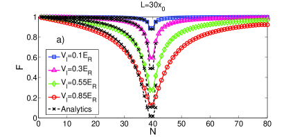
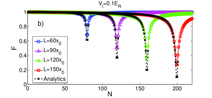
Figure 1: Ground state fidelity (a) as a function of the number of particles $N$, for constant box size $L=30x_{0}$ and lattice wave vector $k=4\pi x_{0}^{-1}/3$ with different lattice amplitudes $V_{l}$. The black crosses are analytical results (for $N\leq M+1$) obtained with first order perturbation theory. Ground state fidelity (b) as a function of $N$, for constant lattice amplitude $V_{l}=0.3E_{R}$ and wave vector $k=4\pi/3$ with different box sizes $L$. See text for details.

Figure 1(a) shows the GSF as a function of the number of particles $N$, for different values of the lattice amplitude. The phase $\phi=0$, i.e., $V_{l}(x)=V_{l}\cos^{2}(kx)$. The size of the box is $L=40\pi/k=30x_{0}$, that is, $M=40$ and we expect the pinning to occur at $N=40$. Indeed we observe a dramatic decrease of fidelity when approaching commensurability, however, the GSF is equal for $N=39$ and $N=40$. One can argue that in the thermodynamic limit there is a single point at which the pinning takes place, and that this anomaly is a consequence of finite size effects. Nevertheless, such finite size effects are important for experimental systems as they occur at the relevant densities. The aforementioned anomaly will be explained in the next subsection using first order perturbation theory. We point out that the GSF obtained with the first order perturbation theory (black crosses) for $N\leq M+1$, developed in Subsection IV.2, is in perfect agreement with numerics for small amplitude $V_{l}=0.1E_{R}$ (blue circles in Fig. 1(a)), for higher amplitudes there are discrepancies between first order perturbation theory and exact numerics in the dip of GSF, while outside of the GSF dip agreement is fairly good for all amplitudes, see Fig. 1(a).

Figure 1(b) shows the GSF as a function of the the number of particles $N$, for different values of $L$ (lattice amplitude is held constant at the value $V_{l}=0.3E_{R}$). We clearly see that GSF decreases in the region of criticality with the increase of $L$, as expected. In the next subsection we will show that at the critical point $F\rightarrow 0$ as $L\rightarrow\infty$.

Let us discuss the boundary effects for a finite-size system. Interestingly, if we use the phase $\phi=\pi/2$ for the lattice, such that $V_{l}(x)=V_{l}\sin^{2}(kx)$, we obtain approximately identical values for the fidelity. In Fig. 2 we show GSF for cosine squared ($\phi=0$ red circles) and sine squared ($\phi=\pi/2$ blue crosses) lattice, these values overlap and come in pairs. This symmetry is lost for phases $\phi$ in between $0$ and $\pi/2$. As an example, Fig. 2 shows GSF as a function of the number of particles for $\phi=\pi/3$ (green squares) and $\phi=\pi/8$ (pink triangles); there is a single point at which GSF has a minimum, either at $N=39$ or at $N=40$. For other phases, in between $\phi=0$ and $\phi=\pi/2$, results are qualitatively and quantitatively similar as for $\phi=\pi/3$ and $\phi=\pi/8$.

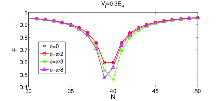
Figure 2: Ground state fidelity as a function of $N$, for different phases $\phi$ of the lattice $V_{l}(x)$. Outside presented interval of $N$, GSF is approximately identical for all phases. See text for details

It is interesting that for a cosine squared lattice with exactly $M$ wells the signature of the pinning occurs at $N=M,M-1$, and that the same values are obtained for a sine squared lattice with $M-1$ wells plus two half-wells. In order to see the differences between different boundary conditions we need to look at another quantity rather than the GSF. We choose to investigate the behavior of the energy (following the experiment Nagerl:10 ), and the single-particle density.

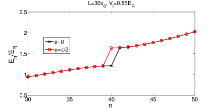
Figure 3: Single particle SP energy spectrum for cosine-squared $\phi=0$ (black crosses) and sine-squared $\phi=\pi/2$ (red circles) lattice, other parameters are $L=30x_{0}$ and $V_{l}=0.85E_{R}$. See text for details.

In Fig. 3 we plot the single-particle (SP) energy spectrum of the potential potential $V_{0}(x)+V_{l}(x)$ for both sine- and cosine-squared lattice. As in Fig. 1(a) the parameters are $L=30x_{0}$ and $k=4\pi x_{0}^{-1}/3$ (which gives $M=40$), and the lattice amplitude is $V_{l}=0.85E_{R}$. We see that the energy spectrum is different for these two lattices. Even though we cannot strictly speak about a gap for a finite size lattice, by observing Fig. 3 we see that the gap-like opening in the spectrum occurs at $n=40$ ($n$ is the index of a single-particle state) for a cosine-squared lattice, whereas for the sine-squared lattice it occurs at $n=39$. These signatures for the pinning transition are intuitively expected when we think of the number of particles versus the number of wells in these two lattices. Even though we speak here about the SP spectrum, the energy gap will be present in many-body excitations of the TG gas as well, because of the FB mapping Girardeau1960 . We emphasize that ’gap’ in SP spectrum occurs for SP states with the same (or approximately the same) wavelength as the lattice wavelength; this fact will be used in Section V.

We now turn to the single-particle densities $\rho(N,x)=\sum_{n=1}^{N}|\phi_{n}(x)|^{2}/N$, which are plotted in Fig. 4 for the cosine- (a) and the sine-squared (b) lattice, in comparison with the density $\rho_{0}(N,x)=\sum_{n=1}^{N}|\psi_{n}(x)|^{2}/N$, and the lattice maxima and minima (parameters are $N=M=40$, $V_{l}=0.55E_{R}$ and $L=30x_{0}$). We see that in both cases the density maxima occur at the lattice minima as expected; the two cases differ at the boundary which is reflected in the energy spectrum but not in the GSF.

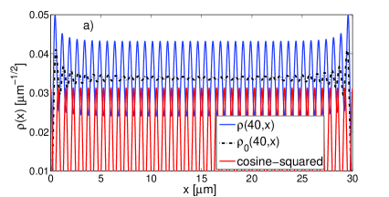
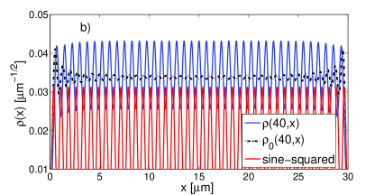
Figure 4: Single particle density $\rho(N,x)$ obtained from the many-body ground states of $N$ atoms in $V_{0}(x)+V_{l}(x)$ potential (a) $\rho(40,x)$ (blue line) in cosine-squared lattice (red line) and (b) $\rho(40,x)$ (blue line) in sine-squared lattice (red line). For reference we plot the corresponding densities $\rho_{0}(N,x)$ of $N$ atoms in the ground state of $V_{0}(x)$ trap (black doted line). See text for details.

In Fig. 5 (a) we show the inset of the density $\rho(N=M,x)$ (red crosses) vs. two nearby densities $\rho(N=M-1,x)$ (blue circles) and $\rho(N=M+1,x)$ (green squares) in the cosine-squared lattice (blue doted line). We clearly see that the probability for particles to ’sit’ at the minima of the cosine-squared lattice is the highest for $N=M$ atoms (also, the probability for the atoms to sit at potential maxima is the lowest for $N=M$ atoms). This observation confirms the indication given by SP energy spectrum in Fig.2 regarding where the pinning takes place in the finite size system. In Fig. 5 (b) we show the same quantities for the sine-squared lattice. We see that the signature of pinning is strongest at $N=M-1$ consistent with the single-particle spectrum.

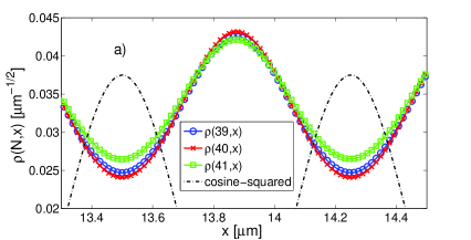
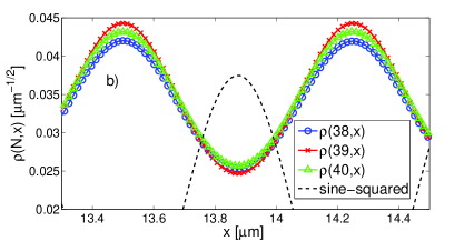
Figure 5: Single particle density. (a) $\rho(40,x)$ (red cross) and two nearby densities $\rho(39,x)$ (blue circles) and $\rho(41,x)$ (green squares) in cosine lattice (blue doted line). (b) $\rho(39,x)$ (red crosses) and two nearby densities $\rho(38,x)$ (blue circles) and $\rho(40,x)$ (green triangles) in sine lattice (blue doted line). A smaller range of axis is chosen to provide good visibility. See text for details.

We see that the energy and the single particle density can distinguish between different types of boundary conditions, whereas the GSF is less sensitive to these effects. The GSF has an advantage over the energy spectrum in the thermodynamic limit where it dramatically shows where the pinning takes place for an infinitesimally small lattice amplitude.

IV.2 Analysis of GSF via 1st order perturbation theory

In this subsection we study the GSF in the context of the pinning phase transition for the box potential via stationary first-order perturbation theory. Unperturbed states are the SP basis of $V_{0}(x)$ i.e $\psi_{n}(x)=\sqrt{(2/L)}\sin(n\pi x/L)$. For the moment let us focus on the cosine-squared lattice $V_{l}(x)=V_{l}\cos^{2}(M\pi x/L)$, which we treat as the small stationary perturbation and denote SP basis of $V_{0}(x)+V_{l}(x)$ as $\phi_{n}(x)$. To first order in the lattice amplitude, the single-particle states of the potential $V_{0}(x)+V_{l}(x)$ are

$$\phi_{i}(x)\propto\psi_{i}(x)+a_{2M-i}\psi_{2M-i}(x)+a_{2M+i}\psi_{2M+i}(x),$$ (9)

where $i\in\{1,\ldots,M-1,M+1,\ldots,2M-1\}$; the case $i=M$ is treated separately. This interval of indices $i$ cover all particle numbers of interest i.e $N=1,\ldots,2M-1$, and the criticality region $N\sim M$ is in the center of that interval. The coefficients are given by $a_{2M-i}=V_{l}/[4(E_{2M-i}-E_{i})]$ and $a_{2M+i}=V_{l}/[4(E_{2M+i}-E_{i})]$ where $E_{i}$ is the SP energy of $i$-th state in the $V_{0}(x)$ potential. Since $E_{i}=(i/M)^{2}E_{R}$ we can write

$$a_{2M\mp i}=\frac{M}{16(M\mp i)}\frac{V_{l}}{E_{R}}.$$ (10)

The coefficient $a_{2M+i}$ in Eq. (9) can be ignored because of the denominator in Eq. (10), i.e., for $i\neq M$

$$\phi_{i}(x)\approx\frac{\psi_{i}(x)+a_{2M-i}\psi_{2M-i}(x)}{\sqrt{1+|a_{2M-i}|^{2}}},$$ (11)

where we have normalized the wave function. We see that perturbation will be most dominant when $i=M-1$ and $i=M+1$.

For $i=M$, the first-order perturbation theory gives $\phi_{M}(x)\propto\psi_{M}(x)+a_{3M}\psi_{3M}(x)$, where $a_{3M}=V_{l}/[4(E_{3M}-E_{M})]=V_{l}/32E_{R}$ is sufficiently small for a weak lattice $V_{l}/E_{R}\ll 1$, and we can write

$$\phi_{M}(x)\approx\psi_{M}(x).$$ (12)

In fact, this relation will hold even for deeper lattices as long as $V_{l}/32E_{R}\ll 1$.

In order to calculate the ground state fidelity $F=|\det{\bf A}|^{2}$ we need to evaluate the matrix elements $A_{ij}=\int\psi_{i}^{*}(x)\phi_{j}(x)dx$ [see Eqs. (5) and (6)]. We first consider the case $N<M$. We use Eqs. (11) and (12) to get matrix elements $A_{ij}$ within first order perturbation theory:

$$A_{ij}\approx\frac{\delta_{ij}+a_{2M-j}\delta_{i,2M-j}}{\sqrt{1+|a_{2M-j}|^{2}}},$$ (13)

where $i,j=1,\ldots,N$. If $N<M$, then the second delta term in (13) is zero, and the matrix (13) is diagonal $A_{ii}=(\sqrt{1+|a_{2M-i}|^{2}})^{-1}$. Thus, the GSF ($N<M$) is

$$F\approx\prod_{i=1}^{N}|A_{ii}|^{2}\approx\prod_{i=1}^{N}\frac{1}{1+|a_{2M-i}|^{2}}$$ (14)

Since the coefficients $|a_{2M-i}|^{2}$ rise quadratically as $i$ approaches $M$, we understand the behavior of GSF when $N$ approaches $M$ from below, which was observed numerically in Fig. 1 (a) and (b). In Fig. 1(a) we plot results of Equation (14) (black crosses), agreement with exact numerical results is excellent for small amplitudes, i.e, $V_{l}=0.1E_{R}$ in Fig. 1(a) (blue squares), for larger amplitudes agreement is good outside the dip of GSF, while we see discrepancies in the dip, resulting from first order perturbation theory are systematically lower than exact numerics.

The case $N=M$ is straightforward due to $A_{MM}\approx 1$, and for $N=M$ the GSF becomes

$$F\approx\prod_{i=1}^{M-1}\frac{1}{1+|a_{2M-i}|^{2}}|A_{MM}|^{2},$$ (15)

which is identical to the value for $N=M-1$ (see Eq. (14)), which explains our numerical observation. This is an interesting observation. The GSF will decrease when first order perturbation is the most effective. We expect it to be the most effective at commensurability, $N=M$. However, the coefficient at $N=M-1$ contributes the most in this sense, whereas for $N=M$ the perturbation on the SP eigenstates (which is reflected onto the many body eigenstates via FB mapping) is essentially negligible.

If we enlarge the box to new size e.g $L^{\prime}=2L$, and we keep the lattice wave vector constant $k=M\pi/L$, we have $M^{\prime}=2M$, and the fidelity dip moves to $N=2M-1$ and $N=2M$, and decreases in value because the new coefficient $a_{M^{\prime}}=2a_{M}$, which gives smaller product terms in equation (14). This explains results of Fig 1(b) where we vary system size $L$.

The first-order perturbation theory also provides an explanation for the influence of the phase $\phi$. For example, for the sine-squared lattice, because $\cos^{2}(kx)=1-\sin^{2}(kx)$, the integrals appearing in the perturbation expansion are

$$\int\psi_{i}^{*}(x)\cos^{2}(kx)\psi_{j}(x)dx=-\int\psi_{i}^{*}(x)\sin^{2}(kx)\psi_{j}(x)dx,$$

and the coefficients change sign, wave functions differ, but the GSF (14) depends on absolute squares of these coefficients and is insensitive to this phase. This explains results of Fig. 2 for cosine-squared and sine-squared lattice (red circles and blue crosses). For some arbitrary phase value between $0$ and $\pi/2$, the main difference is that equations (9) and (12) will no longer hold and more coefficients are needed in expansion of $\phi_{i}(x)$ in terms of $\psi_{i}(x)$, especially for $i\sim M$, which breaks the symmetry between $N=M$ and $N=M-1$ cases.

Let us finally discuss the $N=M+1$ case for the cosine-squared lattice. Matrix ${\bf A}$ acquires two off diagonal elements $A_{M+1,M-1}$ and $A_{M-1,M+1}$ with the following property

$$A_{M+1,M-1}=-A_{M-1,M+1}\approx\frac{a_{M+1}}{\sqrt{1+|a_{M+1}|^{2}}},$$ (16)

due to Eq. (10). In this case the determinant of matrix (13) becomes

$$\det{\bf A}\approx\prod_{i=1}^{M-2}A_{ii}A_{MM}(A_{M-1,M-1}A_{M+1,M+1}-A_{M+1,M-1}A_{M-1,M+1}).$$

Due to (10) and (16) we have $(A_{M-1,M-1}A_{M+1,M+1}-A_{M+1,M-1}A_{M-1,M+1})\approx 1$, and since $A_{MM}\approx 1$, we finally get that determinant of matrix (13) for $M+1$ particles is

$$\det{\bf A}\approx\prod_{i=1}^{M-2}A_{ii}.$$

From the last relation we see that the ground state fidelities for $N=M+1$ and $N=M-2$ particles are approximately equal (see Eq. (14)). In Fig. 1(a) we plot these results for $N=(M,M+1)$ particles (black crosses) in addition to GSF for $N<M$. One could proceed to other values of $N>M+1$ in the same fashion and analyze the GSF via perturbation theory.

V The Pinning transition of the Tonks-Girardeau gas in the harmonic oscillator: ground state fidelity

In this section we study the pinning transition in the experimentally relevant harmonic oscillator (HO) potential Nagerl:10

$$V_{0}(x)=\frac{m\omega_{0}^{2}x^{2}}{2}.$$ (17)

We choose parameters following the experiment in Ref. Nagerl:10 , i.e., the atoms inside the trap are caesium atoms, ¹³³Cs. The optical lattice is $V_{l}(x)=V_{l}\sin^{2}(kx)$ with $k=1.88\pi x_{0}^{-1}$ where $x_{0}=1\mu$m and the wavelength of the lattice is $\lambda=1064$nm. Lattice amplitude and all other energies are in units of the recoil energy $E_{R}=(\hbar k)^{2}/(2m)$.

In Fig. 6(a) we plot the ground state fidelity as a function of number of particles for different values of the lattice amplitude $V_{l}$. The harmonic oscillator frequency is $\omega_{0}/2\pi=25$Hz (similar to the frequency used in experiment $\omega_{exp}/2\pi=22(3)$Hz Nagerl:10 ). We see for all amplitudes $V_{l}$ that GSF first decreases smoothly, in a similar fashion as in the infinitely deep box in Fig. 1(a) and (b). Then GSF decreases faster until it reaches first minimum at $N\approx 50$ after which it develops oscillations with deeper minima. For smaller amplitudes $V_{l}=0.15E_{R}$ (green circles) and $V_{l}=0.45E_{R}$ (blue x’s) the oscillations have a global minimum at $N\approx 60$, and after that the GSF starts to rise, as expected, but at a slower rate compared to the rate of decrease towards the first minimum, in contrast to the square well. For higher amplitude $V_{l}=0.9E_{R}$(red squares) GSF is effectively zero i.e $F\approx 0$ for interval of $N$’s between $N\sim 60$ and $N\sim 70$, with the slow increase of average GSF for $N$ above $70$. Finally, for still higher amplitude $V_{l}=1.4E_{R}$ (black diamonds) (similar to the amplitude used in experiment $V_{exp}=1.5(1)E_{R}$ Nagerl:10 ) GSF drops to values slightly above zero already for $N\approx 45$ and after a small bump we see that $F\approx 0$ from $N\sim 60$ to $N\sim 110$; above $N\sim 110$ GSF slowly rises and develops oscillations (not shown) similar to GSF for $V_{l}=0.9E_{R}$(red squares).

In Fig. 6(b) we plot the ground state fidelity $F$ as a function of $N$ for different values of the harmonic oscillator frequency $\omega_{0}$ with constant lattice amplitude $V_{l}=0.45E_{R}$. We see, as expected, that the pinning transition occurs for larger $N$, and the fidelity dip lowers.

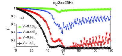
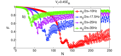
Figure 6: Ground state fidelity for the pinning transition in a harmonic oscillator potential. (a) GSF as a function of number of particles $N$ for different lattice amplitudes $V_{l}$ with constant frequency $\omega_{0}/2\pi=25$Hz. (b) GSF as a function of $N$ for different $\omega_{0}$ with constant $V_{l}=0.45E_{R}$. See text for details.

We point out that the results of Fig. 6(a), obtained for $\gamma\gg 1$, are in excellent agreement with the experimental results of Ref. Nagerl:10 , obtained for large but finite $\gamma$, where it is said that commensurability of superfluid phase and the lattice is best fulfilled when there are about $N\sim 60$ atoms in the central tube. We see in Fig. 6(a) for all amplitudes GSF shows enhanced sensitivity and strongest decay in the region $N\sim 60$.

In order to understand these results, we need to define the commensurability of the Tonks-Girardeau gas and the applied optical lattice. This is not straightforward because of the inhomogeneous atomic density in the ground state of the harmonic oscillator potential. We draw upon the results of Section IV, where the GSF had a minimal value when the unperturbed $N$th SP state entering the $N$-particle ground state via Eq. (4), had the same wavelength as the optical lattice. In the case of the harmonic trap (17), the asymptotic expansion of SP states $\psi_{n}(x)$ for $n\gg 1$ is

$$\psi_{n}(x/a_{0})\propto\cos(\sqrt{2n}x/a_{0}-n\pi/2),$$ (18)

where $a_{0}=\sqrt{\hbar/m\omega_{0}}$. This provides us with the dominant wavelength of the $n$-th SP state. We estimate that the pinning occurs when

$$k\approx\sqrt{2N}/a_{0},$$ (19)

which yields

$$N_{pinn}\approx\frac{k^{2}\hbar}{2m\omega_{0}}$$ (20)

for the number of particles where pinning occurs. Eq. (20) is obtained for $n\gg 1$; in experiments one usually has $N>30$. In addition, we stress that Eq. (20) is in agreement with Ref. buchler , where the pinning transition is said to occur for such $N$ that the peak density of the superfluid phase, obtained with Thomas Fermi approximation for $\gamma\gg 1$, is equal to the commensurate density $n_{c}=2/\lambda$. For $\omega/2\pi=25$Hz our estimate yeilds $N_{pinn}\sim 50$, which explains the drop in the GSF observed in Fig. 6(a). Equation (20) also explains the positions of the first minima of GSF in Fig. 6(b) since it gives $N_{pinn}\sim\{38,52,75,130\}$ for $\omega_{0}/2\pi=\{35,25,17.5,10\}$Hz, respectively, in fair agreement with exact numerical results. Again, as we make the system larger, the minimum value of GSF decreases which is consistent with the decrease of GSF at criticality in the thermodynamic limit.

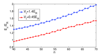
Figure 7: Single particle energy spectrum of harmonic trap with the lattice $V_{0}(x)+V_{l}(x)$, for two values of amplitude $V_{l}=1.4E_{R}$ (blue circles) and $V_{l}=0.45E_{R}$ (red triangles). See text for details.

Besides the GSF, it is instructive also to look into the single particle energy spectrum plotted in Fig. 7 for $V_{0}(x)+V_{l}(x)$ with the amplitudes $V_{l}=0.45E_{R}$ (red triangles) and $V_{l}=1.4E_{R}$ (blue circles). We see that for $V_{l}=0.45E_{R}$ (red triangles) at $n\sim 50$ and larger values a series of ’gaps’ open up in the sense that at some $N$ values the excitations of the TG gas from the ground state cost more energy.

These results can also be understood simply in terms of commensurability of the SP density of the TG gas in the HO potential and the lattice $V_{l}(x)$. SP density of $N$ particles in the ground state of TG gas in $V_{0}(x)$ potential is $\rho_{0}(N,x)=\sum_{n=0}^{N-1}|\psi_{n}(x)|^{2}$. This function is inhomogeneous with maximum value (peak density) at $x=0$ (we now ignore the small auxillary oscillations which can lead to the local minimum for $x=0$ depending on the parity of $n=N-1$th state). When we increase $N$ (starting from $N=1$), the first part of the density $\rho_{0}(N,x)$ that approaches the commensurability condition $n_{c}=2/\lambda$, is the central part i.e for $\rho_{0}(N,0)$. Thus the first ’gap’, and first minima of GSF, will appear for $N_{pinn}$ with property $\rho_{0}(N_{pinn},0)\approx n_{c}$, in accordance with Ref. buchler and Equation (20). Adding more particles, i.e $N>N_{pinn}$, leads to $\rho_{0}(N,0)>n_{c}$ but now in some regions left and right from $x=0$, the density becomes commensurate with lattice i.e $\rho_{0}(N,-d)\approx n_{c}$ and $\rho_{0}(N,d)\approx n_{c}$, for some $d>0$, and pinning still occurs, i.e, additional ’gaps’ in SP spectrum are present and GSF still lowers. The distance $d$ increases with the increase of $N$ and commensurability condition is satisfied for regions further towards the edges of the trap $V_{0}(x)$. The fraction of the atomic cloud commensurate with the lattice gets smaller and as a consequence the GSF slowly increases. Oscillations are present due to many fine details such as the interplay of symmetry of the lattice and the symmetry of the $\psi_{N}(x)$ states.

VI The Loschmidt echo and out of equilibrium dynamics: sudden quench with optical lattice

In this section we look for signatures of the pinning transition in the non-equilibrium dynamics of TG gas, initially in ground state of some trapping potential $V_{0}(x)$, after optical lattice $V_{l}(x)$ is suddenly turned on. This is an example of a sudden ’quench’. Before the quench with the lattice potential, the gas is in the equilibrium ground state $|\Psi_{0}\rangle$ of Hamiltonian $\hat{H}_{0}$, see (1). At $t=0$ we suddenly turn on the lattice potential $V_{l}(x)$ and an out-of-equilibrium many body state $|\Phi(t)\rangle=\exp[-i(\hat{H_{0}}+V_{l}(x))t/\hbar]|\Psi_{0}\rangle$ starts to evolve, where $|\Phi(0)\rangle=|\Psi_{0}\rangle$ is the initial condition. We would like to develop a quantitative understanding of the out of equilibrium dynamics which is encoded in this state. Conveniently, the mapping theorem also holds for time dependent states, and the quenched state $|\Phi(t)\rangle$ can be constructed using a Slater determinant of time evolving single particle states such that $|\Phi(t)\rangle=\frac{1}{\sqrt{N}!}\prod_{1\leq i<j\leq N}\mbox{sgn}(x_{i}-x_{j})\det_{n,j=1}^{N}\left[\psi_{n}(x_{j},t)\right]$. The single particle states $\psi_{n}(x_{j},t)$ are out of equilibrium, and obtained by solving $i\hbar\partial_{t}\psi_{n}(x,t)=\left[-\hbar^{2}/(2m)\partial_{x}^{2}+V_{0}(x)+V_{l}(x)\right]\psi_{n}(x,t)$ with initial conditions $\psi_{n}(x,0)=\psi_{n}(x)$ where $\psi_{n}(x)$ are the initial single particle states (SP) which are used to construct the unperturbed ground state $|\Psi_{0}\rangle$ i.e SP states of $V_{0}(x)$ potential.

A prototypical quantity to calculate for a system perturbed out of equilibrium is the so-called Loschmidt echo Gorin , which is defined as

$$L(t)=|\langle\Psi_{0}|\exp(i\hat{H}_{0}t/\hbar)\exp[-i(\hat{H}_{0}+V_{l}(x))t/\hbar]|\Psi_{0}\rangle|^{2}.$$

It is a measure of the sensitivity of the system to the quench protocol, which in this case is simply the application of the external lattice potential to the initial Tonks gas equilibrium state. Despite it’s mathematical simplicity, it conveys a great deal of information about the many-body system under scrutiny, such as universal behavior at criticality Zanardi:06 and important information on the thermalization of observables. Closed formulas for the echo are, in general, very difficult to obtain. For a Tonks-Girardeau gas, the Loschmidt echo was recently computed in a relatively straightforward way Lelas .

Since $\hat{H}_{0}|\Psi_{0}\rangle=\Omega_{0}|\Psi_{0}\rangle$, where $\Omega_{0}$ is ground state energy of TG gas in $V_{0}(x)$ trap, we get

$$L(t)=|\langle\Psi_{0}|\exp[-i(\hat{H}_{0}+V_{l}(x))t/\hbar]|\Psi_{0}\rangle|^{2}=|\langle\Psi_{0}|\Phi(t)\rangle|^{2}.$$ (21)

Relation (21) shows that in our case the Loschmidt echo (LE) is equivalent to the survival probability i.e probability that system will be in the initial state at the time $t$ after the quench. We will interchangeably use the terms Loschmidt echo and survival probability.

The Fermi-Bose mapping theorem is valid for time dependent wave functions thus LE can be written in a form convenient for calculation, analogous to the calculation of the static fidelity,

$$L(t) = |\frac{1}{N!}\int dx_{1}\cdots dx_{N}\sum_{\sigma_{1}}(-)^{\sigma_{1}}\prod_{i=1}^{N}\psi^{*}_{\sigma_{1}(i)}(x_{i},0)\sum_{\sigma_{2}}(-)^{\sigma_{2}}\prod_{j=1}^{N}\psi_{\sigma_{2}(j)}(x_{j},t)|^{2}$$ (22)

$$= |\det\mathbf{A}(t)|^{2}$$

and $\mathbf{A}(t)$ is the time dependent matrix containing overlaps between static SP states of the $V_{0}(x)$ potential i.e $\psi_{i}(x,0)$ and SP states $\psi_{i}(x,t)$ evolved in perturbed potential $V_{0}(x)+V_{l}(x)$

$$A_{ij}(t)=\int\psi_{i}^{*}(x,0)\psi_{j}(x,t)dx.$$ (23)

Equations (22) and (23) were recently used to study the long time behavior of many-particle quantum decay delCampo . The LE of the TG gas is formally equivalent to the corresponding echo for a gas of non-interacting fermions Goold2011 . The Loschmidt echo of one-dimensional interacting Bose gases was recently related Lelas to series of experiments Hofferberth2007 ; Hofferberth2008 ; Kruger2010 and theoretical studies Polkolnikov2006 ; Gritsev2006 ; Bistritzer2007 ; Burkov2007 ; Mazets2008 ; Stimming2011 on interference between split parallel 1D Bose systems.

VI.1 Infinitely deep well

In this subsection we use (22) and (23) to explore the LE of a TG gas after a sudden quench with optical lattice $V_{l}(x)$, i.e at $t=0$ we suddenly turn on the lattice and leave it on. Before the quench TG gas is in ground state $|\Psi_{0}\rangle$ of infinitely deep well (8) potential $V_{0}(x)$. In this subsection we use same units and parameters as in section IV.

In Fig. 8 we show Loschmidt echo $L(t)$, as a function of time for different numbers of particles $N$ obtained with exact numerical evolution, for optical lattice $V_{l}(x)=0.55E_{R}\cos^{2}(4\pi xx_{0}^{-1}/3)$. Size of the well $L=30x_{0}$. Number of lattice wells is $M=40$. That set of parameters is the same as the one we used for ground state fidelity $F$ in Fig. 1(a) denoted with red circles. We see that properties of $F$ are reflected in LE. Values of LE goes in pairs, i.e, curves are approximately equal for $N=M-j$ and $N=M+j-1$ particles, with $j=1,\ldots,M-1$. Decay of Loschmidt echo is strongest and fastest close to criticality, i.e, for $N=39$ and $N=40$ particles (red circles and red solid line). In addition, the oscillations get slower as we approach criticality.

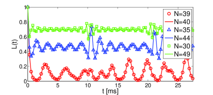
Figure 8: Loschmidt echo $L(t)$ for different particle numbers $N$ in the infinitely deep box potential. Optical lattice $V_{l}(x)$ has $40$ minima, i.e, $M=40$ lattice wells. LE reflects properties of GSF, i.e, decay is strongest for $N=(M-1,M)$, and Loschmidt echo appears in pairs. The frequency of revivals decreases as we approach criticality. See text for details.

In order to understand the results of Fig. 8 we use relations (10)-(12) to write expansion of the unperturbed SP states of $V_{0}(x)$ in terms of the perturbed SP states of $V_{0}(x)+V_{l}(x)$ i.e

$$\psi_{i}(x,0)\approx\frac{\phi_{i}(x)-a_{2M-i}\phi_{2M-i}(x)}{\sqrt{1+|a_{2M-i}|^{2}}}.$$ (24)

For $i=1,\ldots,M-1,M+1,\ldots,2M-1$. In case of $i=M$ we get

$$\psi_{M}(x,0)\approx\phi_{M}(x).$$ (25)

Using relation (24) we get time evolution of $\psi_{j}(x,t)$ after the quench

$$\psi_{j}(x,t)\approx\frac{\exp(-iE_{j}^{l}t/\hbar)\phi_{j}(x)-a_{2M-j}\exp(-iE_{2M-j}^{l}t/\hbar)\phi_{2M-j}(x)}{\sqrt{1+|a_{2M-j}|^{2}}},$$ (26)

where $E_{n}^{l}$ are SP energy’s in $V_{0}(x)+V_{l}(x)$ potential. Now we use (24)-(26) in Equations (23) and (22) in order to obtain insight in to the behavior of the Loschmidt echo. The following analysis is very similar to analysis done in subsection IV.2 for the ground state fidelity.

First, we consider the case when the number of particles is less than the number of wells, i.e $N<M$. In this case matrix (23) is diagonal with

$$A_{ii}(t)\approx\frac{\exp(-iE_{i}^{l}t/\hbar)+|a_{2M-i}|^{2}\exp(-iE_{2M-i}^{l}t/\hbar)}{1+|a_{2M-i}|^{2}},$$

and since $L(t)=|\det{\bf A}(t)|^{2}=\det\left[{\bf A}(t){\bf A^{*}}(t)\right]$ we get

$$\L(t)\approx\prod_{i=1}^{N}|A_{ii}(t)|^{2},$$ (27)

where

$$|A_{ii}(t)|^{2}\approx\frac{1+2|a_{2M-i}|^{2}\cos\left[(E_{2M-i}^{l}-E_{i}^{l})t/\hbar\right]+|a_{2M-i}|^{4}}{\left(1+|a_{2M-i}|^{2}\right)^{2}}.$$ (28)

If we use expression (14) for the ground state fidelity ($F$) we get for the Loscmidt echo of $N<M$ particles

$$\L(t)\approx F^{2}\prod_{i=1}^{N}(1+2|a_{2M-i}|^{2}\cos\left[(E_{2M-i}^{l}-E_{i}^{l})t/\hbar\right]+|a_{2M-i}|^{4}),$$ (29)

we see that ground state fidelity is incorporated in LE by construction i.e., that is why the LE reflects it’s properties. Since coefficients $|a_{2M-i}|^{2}$ grow quadratically as $i$ approaches $M$ the most dominant cosine term in (29) is for $i=N$ which leads to the conclusion that the dominant frequency of revivals $\omega_{R}$ for LE of $N<M$ particles is simply related to the SP energy of $V_{0}(x)+V_{l}(x)$ potential through the relation

$$\omega_{R}(N)=\frac{E_{2M-N}^{l}-E_{N}^{l}}{\hbar}.$$ (30)

Now consider the case $N=M$. Going from $N=M-1$ to $N=M$ particles, the matrix (23) remains diagonal due to relation (25), we simply add $A_{MM}(t)\approx\exp(-iE_{M}^{l}t/\hbar)$ on the main diagonal, and since $|A_{MM}(t)|^{2}\approx 1$, we get that the LE for $N=M$ is the same as the LE for $N=M-1$ particles, in accordance with Fig. 8 (red solid line for $N=40$ and red circles for $N=39$ particles).

Now we proceed to the $N=M+1$ case. In this case the matrix (23) obtains two off diagonal elements

$$A_{M+1,M-1}(t)=A_{M-1,M+1}(t)\approx\frac{-a_{M+1}\exp(-iE_{M+1}^{l}t/\hbar)-a_{M-1}\exp(-iE_{M-1}^{l}t/\hbar)}{1+|a_{M+1}|^{2}},$$ (31)

where we used (24) and $|a_{M-1}|=|a_{M+1}|$, see (10). The determinant of the matrix (23) has two terms, the product of diagonal elements and a term arising from two off diagonal elements

$$\det{\bf A}(t)\approx\prod_{i=1}^{M-2}A_{ii}(t)A_{MM}(t)\left[A_{M-1,M-1}(t)A_{M+1,M+1}(t)-A_{M+1,M-1}(t)A_{M-1,M+1}(t)\right].$$

It can be shown that

$$\left[A_{M-1,M-1}(t)A_{M+1,M+1}(t)-A_{M+1,M-1}(t)A_{M-1,M+1}(t)\right]\approx\exp\left[-i(E_{M-1}^{l}+E_{M+1}^{l})t/\hbar\right],$$

which together with $A_{MM}(t)\approx\exp(-iE_{M}^{l}t/\hbar)$, yields

$$L(t)=|\det{\bf A}(t)|^{2}\approx\prod_{i=1}^{M-2}|A_{ii}(t)|^{2}.$$

We conclude that the Loschmidt echoes for $N=M+1$ and $N=M-2$ are approximately the same. We see that the same pattern emerges as with ground state fidelity. The Loschmidt echo values come in pairs, i.e, it is approximately the same for $N=M-j$ and $N=M+j-1$ particles, where $j=1,\ldots,M-1$. Due to this pattern, we can use Eq. (30) to get the dominant revival frequency of Loschmidt echo for other particle numbers $N\geq M$, i.e we can write

$$\omega_{R}(M+j-1)\approx\omega_{R}(M-j),$$ (32)

where $j=1,\ldots,M-1$ and $\omega_{R}(M-j)$ on the right side of Eq. (32) is given by Eq. (30). In order to check the quality of these relations, we plot in Fig. 9 the dominant revival frequency $\omega_{R}(N)$ obtained via (30) and (32) for $N=1,\ldots,2M-2$ particles (for parameters used here $M=40$), together with the most dominant frequency $\omega_{FFT}(N)$ obtained with the Fourier transform of LE; the agreement is excellent. Parameters used to calculate the LE are the same as in Fig. 8.

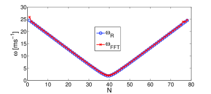
Figure 9: Dominant revival frequency of Loschmidt echo obtained with Eqs. (30) and (32) $\omega_{R}$ (blue circles) and with the Fourier transform of Loschmidt echo $\omega_{FFT}$ (red crosses). Parameters used for calculation of LE are the same as in Fig. 8. See text for details.

VI.2 Harmonic oscillator

In this subsection we use Eqs. (22) and (23) to explore the LE of a TG gas following a sudden quench with optical lattice $V_{l}(x)$; before the quench the TG gas is in the ground state $|\Psi_{0}\rangle$ of harmonic oscillator potential $V_{0}(x)$ (17). In this subsection we use same units and parameters as in Section V.

In Fig. 10 we show the Loschmidt echo following the quench with optical lattice $V_{l}(x)=0.45E_{R}\sin^{2}(1.88\pi x_{0}^{-1}x)$; the system was initially in a ground state of the harmonic oscillator potential with $\omega_{0}/2\pi=25$Hz. Fig. 10(a) is for $N<N_{pinn}$ and Fig. 10(b) is for $N>N_{pinn}$, where $N_{pinn}$ is given by Eq. (20) (for parameters used here $N_{pinn}\approx 52$). We see that properties of GSF (see Fig. 6(a) blue crosses) are reflected in the LE; the average values of the LE are lower for lower GSF. This is a general observation. However, the details of LE dynamics (such as the dominant revival frequency) depend on trapping potential.

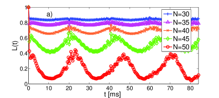
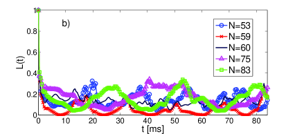
Figure 10: The Loschmidt echo $L(t)$ for different particle numbers $N$. a) LE for particle numbers up to $N<N_{pinn}$. b) LE for $N>N_{pinn}$. See text for details.

In Fig. 11 we illustrate the dominant frequency of the LE (from Fig. 10) obtained with the Fourier transform ($\omega_{FFT}$ blue crosses). We see that $\omega_{FFT}$ is constant for $N\leq N_{pinn}$, and it starts to behave irregularly for $N>N_{pinn}$. We have found numerically that the regular behavior for $N\leq N_{pinn}$ occurs because $\psi_{n}(x,0)$ can be well approximated with

$$\psi_{n}(x,0)\sim A\phi_{n-2}(x)+B\phi_{n}(x)+C\phi_{n+2}(x),$$

where coefficient $B$ is always the largest in magnitude; this yields

$$\omega_{R}(N\leq N_{pinn})\approx 2\omega_{0}$$ (33)

which is also plotted in Fig. 11. For $N>N_{pinn}$ there are many coefficients in the expansion of $\psi_{n}(x,0)$ in terms of $\phi_{n}(x)$ which contribute on equal footing and simple relation (33) does not hold anymore.

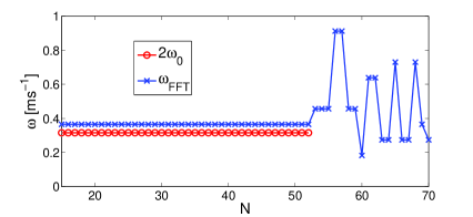
Figure 11: Dominant revival frequency of Loschmidt echo obtained with Eq. (33) $\omega_{R}$ (red circles) and with the Fourier transform of the Loschmidt echo $\omega_{FFT}$ (blue crosses). The parameters used to calculate the LE are the same as in Fig. 10. See text for details.

VII Conclusion

We have studied the pinning quantum phase transition in a Tonks-Girardeau gas, both in equilibrium and out-of-equilibrium, using the ground state fidelity and the Loschmidt echo as diagnostic tools. We have found, both numerically and analytically (within first order perturbation theory), that the ground state fidelity can individuate the region of criticality. The ground state fidelity defined in Eq. (5) has a dramatic decrease when the atomic density approaches the commensurate density of one particle per lattice well. This decrease is a signature of the pinning transition from the Tonks to the Mott insulating phase. We have found that the ground state fidelity of the TG gas in an infinitely deep well potential can be insensitive to finite size effects. The GSF for $N=M-1$ and $N=M$ particles ($M$ denotes number of lattice wells) in cosine-squared (sine-squared) lattice are the same, while the single particle energy spectrum and density show that pinning actually happens for $N=M$ ($N=M-1$, respectively). The GSF has an advantage over the density and single particle energy spectrum in the thermodynamic limit, where it dramatically shows where the pinning takes place for an infinitesimally small lattice amplitude. We have studied the applicability of the fidelity for diagnosing the pinning transition in experimentally realistic scenarios. Our results are in excellent agreement with recent experimental work Nagerl:10 .

We have found that the GSF in a harmonic oscillator potentials shows enhanced sensitivity in a broad region of particle numbers $N\geq N_{pinn}$ (where $N_{pinn}$ is defined in Eq. (20)); at $N\sim N_{pinn}$ GSF has a faster decay and for larger $N$ develops oscillations. This behavior is related to series of ’gaps’ opening at $n\sim N_{pinn}$ in the single particle energy spectrum of the total potential (harmonic oscillator plus optical lattice).

In addition, we have explored the out of equilibrium dynamics of the gas following a sudden quench with a lattice potential potential. We have showed that all properties of the ground state fidelity are reflected in the Loschmidt echo dynamics i.e., in the non equilibrium dynamics of the Tonks-Girardeau gas initiated by sudden quench of the lattice potential. The average value of the Loschmidt echo is lower for lower values of ground state fidelity, regardless of the details of the trapping potential. Details of the Loschmidt echo dynamics, such as dominant revival frequency, depends on the type of trapping potential. We find regular behavior of revivals for all relevant particle numbers in infinitely deep well potential i.e, frequency’s get lower as we approach criticality and can be calculated simply from single particle energy spectrum of the total potential (infinitely deep well plus optical lattice). In the harmonic oscillator potential, the dominant frequency of revivals behaves in a regular way. It is a constant, approximately equal to $2\omega_{0}$ ($\omega_{0}$ is frequency of harmonic trap), until a series of ’gaps’ open in the single particle energy spectrum of the total potential.

- (1) I. Bloch, J. Dalibardi, and W. Zwerger, Rev. Mod. Phys. 80, 885 (2008).
- (2) See Focus on dynamics and thermalization in isolated quantum many-body systems, M.A. Cazalilla and M. Rigol, New. J. Phys. 12, 055006 (2010), and references therein.
- (3) F. Schreck, L. Khaykovich, K.L. Corwin, G. Ferrari, T. Bourdel, J. Cubizolles, and C. Salomon, Phys. Rev. Lett. 87, 080403 (2001); A. Görlitz, J.M. Vogels, A.E. Leanhardt, C. Raman, T.L. Gustavson, J.R. Abo-Shaeer, A.P. Chikkatur, S. Gupta, S. Inouye, T. Rosenband, and W. Ketterle, ibid. 87, 130402 (2001); M. Greiner, I. Bloch, O. Mandel, T.W. Hänsch, and T. Esslinger, ibid. 87, 160405 (2001); H. Moritz, T. Stöferle, M. Kohl, and T. Esslinger, ibid. 91, 250402 (2003); B. Laburthe-Tolra, K.M. O’Hara, J.H. Huckans, W.D. Phillips, S.L. Rolston, and J.V. Porto, ibid. 92, 190401 (2004); T. Stöferle, H. Moritz, C. Schori, M. Kohl, and T. Esslinger, ibid. 92, 130403 (2004).
- (4) T. Kinoshita, T. Wenger, and D.S. Weiss, Science 305, 1125 (2004); B. Paredes, A. Widera, V. Murg, O. Mandel, S. Fölling, I. Cirac, G. V. Shlyapnikov, T. W. Hänsch, and I. Bloch, Nature (London) 429, 277 (2004).
- (5) T. Kinoshita, T. Wenger, and D.S. Weiss, Nature (London) 440, 900 (2006).
- (6) H. P. Büchler, G. Blatter, and W. Zwerger, Phys. Rev. Lett. 90, 130401 (2003).
- (7) E. Haller, R. Hart, M. J. Mark, J. G. Danzl, L. Reichsollner, M. Gustavsson, M. Dalmonte, G. Pupillo and H. C. Nägerl, Nature. 466, 597 (2010).
- (8) P. Zanardi and N. Paunković, Phys. Rev. E. 74, 031123 (2006).
- (9) For reviews see A. Steane, Rep. Prog. Phys. 61, 117 (1998); D. P. DiVincenzo and C. H. Bennett, Nature 404, 247 (2000)
- (10) A. Peres, Phys. Rev. A 30, 1610 (1984).
- (11) R.A. Jalabert and H.M. Pastawski, Phys. Rev. Lett. 86, 2490 (2001).
- (12) Ph. Jacquod, P.G. Silvestrov, and C.W.J. Beenakker, Phys. Rev. E 64, 055203(R) (2001)
- (13) N. R. Cerruti and S. Tomsovic, Phys. Rev. Lett. 88, 054103 (2002).
- (14) T. Prosen, Phys. Rev. E 65, 036208 (2002).
- (15) T. Gorin, T. Prosen, T.H. Seligman, M. Žnidarič, Phys. Rep. 435, 33 (2006).
- (16) M. Girardeau, J. Math. Phys. 1, 516 (1960).
- (17) K. Lelas, T. S̆eva, and H. Buljan, Phys. Rev. A 84, 063601 , (2011).
- (18) C. De Grandi, V. Gritsev, and A. Polkovnikov, Phys. Rev. B. 81 012303 (2010).
- (19) J. Goold, T. Fogarty, M. Paternostro, Th. Busch, Phys. Rev. A 84, 063632 (2011).
- (20) A. del Campo, Phys. Rev. A 84, 012113 (2011)
- (21) S. Hofferberth, I. Lesanovsky, B. Fischer, T. Schumm, J. Schmiedmayer, Nature (London) 449, 324 (2007).
- (22) S. Hofferberth, I. Lesanovsky, B. Fischer, T. Schumm, J. Schmiedmayer, Nature Physics 4, 489 (2008).
- (23) P. Krüger, S. Hofferberth, I.E. Mazets, I. Lesanovsky, and J. Schmiedmayer, Phys. Rev. Lett. 105, 265302 (2010).
- (24) A. Polkovnikov, E. Altman, and E. Demler, Proc. Natl. Acad. Sci. U.S.A. 103, 6125 (2006).
- (25) V. Gritsev, E. Altman, E. Demler, and A. Polkovnikov, Nature Physics 2, 705 (2006).
- (26) R. Bistritzer and E. Altman, Proc. Natl. Acad. Sci. U.S.A. 104, 9955 (2007).
- (27) A.A. Burkov, M.D. Lukin, and E. Demler, Phys. Rev. Lett. 98, 200404 (2007).
- (28) I.E. Mazets and J. Schmiedmayer, Eur. Phys. J. B 68, 335 (2009).
- (29) H.-P. Stimming, N.J. Mauser, J. Schmiedmayer, and I.E. Mazets, Phys. Rev. A 83, 023618 (2011).