Cross-Layer Optimization of Two-Way Relaying for Statistical QoS Guarantees

Abstract

Two-way relaying promises considerable improvements on spectral efficiency in wireless relay networks. While most existing works focus on physical layer approaches to exploit its capacity gain, the benefits of two-way relaying on upper layers are much less investigated. In this paper, we study the cross-layer design and optimization for delay quality-of-service (QoS) provisioning in two-way relay systems. Our goal is to find the optimal transmission policy to maximize the weighted sum throughput of the two users in the physical layer while guaranteeing the individual statistical delay-QoS requirement for each user in the datalink layer. This statistical delay-QoS requirement is characterized by the QoS exponent. By integrating the concept of effective capacity, the cross-layer optimization problem is equivalent to a weighted sum effective capacity maximization problem. We derive the jointly optimal power and rate adaptation policies for both three-phase and two-phase two-way relay protocols. Numerical results show that the proposed adaptive transmission policies can efficiently provide QoS guarantees and improve the performance. In addition, the throughput gain obtained by the considered three-phase and two-phase protocols over direct transmission is significant when the delay-QoS requirements are loose, but the gain diminishes at tight delay requirements. It is also found that, in the two-phase protocol, the relay node should be placed closer to the source with more stringent delay requirement.

I Introduction

The explosive developments of wireless communication have brought us into a new era where higher data transmission rates and diverse quality-of-service (QoS) provisioning are desperately expected. Real-time applications, such as voice over IP and video streaming, which are highly delay-sensitive, need reliable QoS guarantees. The design merely at the physical layer may not ensure the desired QoS requested by the service from upper layers. Only through the interaction and optimization between different layers can such QoS guarantees be fulfilled. This kind of cross-layer approach relaxes the layering architecture of the conventional network model and brings remarkable performance enhancement, which in turn could result in high complexity. Therefore, to develop efficient cross-layer methods with small information flows between layers is interesting from both theoretical and practical perspectives.

Recently, two-way relaying has appeared as an advanced relay technique to significantly boost the spectral efficiency in wireless networks [2, 3, 4, 5]. The notion of two-way relaying is to apply the principle of network coding at the physical layer so that only three or two time slots are needed when a pair of nodes exchange information via a relay node, while the conventional one-way relaying requires four time slots. Most previous efforts on two-way relaying have focused on the design and optimization merely in physical layer, such as analysis of capacity bounds [5, 6], adaptive network-coded constellation mapping [7], joint channel coding and network coding design [8, 9], precoding design with multiple antennas [10], and resource allocation for throughput maximization in OFDMA networks [11, 12, 13, 14]. Certainly, it is desirable and promising to investigate the cross-layer design and optimization of two-way relay architecture for QoS provisioning. To our best knowledge, only two attempts have been made to study the cross-layer design for two-way relaying [15, 16]. Specifically, [15] and [16] characterized the queue stability region for infinite backlogs with the XOR and superposition-coding based decode-and-forward (DF) protocols, respectively. Nevertheless, having stable queue does not provide optimality in delay performance.

Motivated by the needs for bounded delay performance and small inter-layer information flows, we adopt the concept of QoS exponent and consider the cross-layer optimization of two-way relay systems for statistical delay QoS guarantees in this work. The QoS exponent is used to characterize the statistical delay performance metric, namely, the delay-bound violation probability, and is the only requested information exchanged between the datalink layer and the physical layer [24]. As a result, our work builds on the information theory to capture the performance limits at the physical layer and the statistical QoS theory to model the delay performance from upper layers. Specifically, we aim to find the optimal transmission strategies to maximize the weighted sum rate while guaranteeing the individual statistical delay QoS requirement for each source node. Through integrating the theory of effective capacity [25], we convert this problem into a weighted sum effective capacity maximization problem. After that, the optimal power and rate adaptation policies as functions of both the network channel state information (CSI) and the delay-QoS constraints are developed.

The main contributions and results of this paper are summarized as follows: We formulate the cross-layer optimization problem for statistical QoS guarantees in two-way relay systems as weighted sum effective capacity maximization. This problem is shown to be convex. Furthermore, we propose the optimal transmission strategies with joint power and rate adaptation for both three-phase and two-phase two-way relaying schemes. Particularly, for the two-phase protocol, the optimal channel state partition criterion for successive decoding in the multiple-access (MAC) phase is derived. Numerical results show that, compared with the conventional two-way direct transmission, the considered three-phase and two-phase two-way relay protocols can significantly improve the average throughput when the statistical delay QoS requirements are loose. However, as delay constraints become stringent, the performance gain reduces, and eventually all the throughputs approach zero. It is also demonstrated that, under the same delay-QoS constraint, the three-phase protocol has higher weighted sum effective capacity than the two-phase protocol in high signal-to-noise ratio (SNR) regime, but has lower weighted sum effective capacity than the two-phase protocol in low SNR regime. Moreover, we show that the three-phase protocol has superiority over the two-phase protocol when the relay is extremely adjacent to either of the sources. Meanwhile, it is better to place the relay closer to the source with more stringent delay requirement for the two-phase protocol.

The remainder of this paper is organized as follows. Section II introduces some preliminaries on statistical QoS guarantees and the related work. Section III presents the system model and demonstrates our problem formulation. In Section IV and Section V, we propose the optimal transmission strategies for the three-phase and two-phase transmission, respectively. Numerical results are provided in Section VI to verify the effectiveness of the proposed policies. Finally, we conclude the paper in Section VII.

II Background on Statistical QoS Guarantees and Related Work

II-A Preliminaries on Statistical QoS Guarantees

Due to the time-varying nature of wireless channels, it is infeasible to guarantee the hard delay bound for real-time traffic. Therefore, statistical QoS metric, in the form of the delay-bound violation probability, is commonly used to characterize the diverse delay-QoS requirements.

Based on the large deviation principle, the author in [24] showed that under sufficient conditions, the stationary queue length process $Q(t)$ converges in distribution to a random variable $Q(\infty)$ satisfying that

$$-\lim_{Q_{th}\to\infty}\frac{\ln(Pr\{Q(\infty)>Q_{th}\})}{Q_{th}}=\theta,$$ (1)

where $\theta>0$ is called QoS exponent, denoting the exponential decay rate of the distribution, and $Q_{th}$ is the queueing length bound. According to the above equation, the probability that the steady-state queue length exceeds a certain bound $Q_{th}$ can be approximated by

$$Pr\{Q(\infty)>Q_{th}\}\approx e^{-\theta Q_{th}}.$$ (2)

Similarly, the delay-bound violation probability can be stated as

$$Pr\{D>D_{th}\}\approx e^{-\theta\varphi(\theta)D_{th}},$$ (3)

where $D$ and $D_{th}$ denote the queueing delay and delay bound, respectively, and $\varphi(\theta)$ is known as the effective bandwidth of the arrival process under a given $\theta$. From (3) we can conclude that the violation probability for a given delay bound is characterized by the QoS exponent $\theta$. Therefore, the dynamics of $\theta$ correspond to different delay requirements. Obviously, a smaller $\theta$ implies a looser delay QoS constraint, while a larger $\theta$ means a more strict delay QoS constraint. In particular, when $\theta\rightarrow 0$, the queueing system can tolerate an arbitrary delay, whereas when $\theta\rightarrow\infty$, the system cannot allow any delay.

Inspired by the theory of effective bandwidth, Wu and Negi introduced effective capacity in [25], which is defined as the maximum constant arrival rate that a given service process can support in order to guarantee a statistical QoS requirement specified by $\theta$. Analytically, the effective capacity, denoted by $\mathscr{C}_{\emph{e}}(\theta)$, can be given by

$$\mathscr{C}_{\emph{e}}(\theta)=-\lim_{t\to\infty}\frac{1}{\theta t}\ln\big{(}\mathbb{E}\big{[}e^{-\theta S[t]}\big{]}\big{)},$$ (4)

where $S[t]=\sum_{i=1}^{t}R[i]$ is the time-accumulation of the service process, and $\{R[i],i=1,2,\ldots\}$ corresponds to the discrete-time stationary and ergodic stochastic service process. $\mathbb{E}[\cdot]$ denotes the expectation.

Under the assumption that the block fading channel is independent and identically distributed (i.i.d) over each time frame, the sequence $\{R[i]\}$ is uncorrelated. Then the effective capacity can be rewritten as

$$\mathscr{C}_{\emph{e}}(\theta)=-\frac{1}{\theta}\ln\big{(}\mathbb{E}\big{[}e^{-\theta R[i]}\big{]}\big{)}.$$ (5)

Since the average arrival rate is equal to the average service rate when the queue is in steady state, effective capacity can also be regarded as the maximum throughput subject to a delay-QoS constraint. In particular, as $\theta\rightarrow 0$, the optimal effective capacity approaches the ergodic capacity of the channel. On the other hand, as $\theta\rightarrow\infty$, the optimal effective capacity is drawing to the zero-outage capacity of the channel.

II-B Related Work on Delay-QoS Provisioning

Delay-constrained cross-layer optimization has been studied extensively in a variety of wireless networks [17, 18, 19, 20, 21, 22, 23, 27, 28]. For instance, [17] focused on the characterization of the stability region and throughput optimal control for one-way relay systems. The delay minimization problem based on power control and relay selection for one-way relay systems with multiple antennas was considered in [18]. Joint power and subcarrier allocation for conventional OFDMA networks with heterogeneous delay constraints was explored in [19, 20]. Power allocation with statistical delay-QoS provisioning for conventional point-to-point, one-way relaying, and multiuser systems was studied in [21], [22] and [23], respectively. Authors in [27] proposed an optimal scheduling algorithm for time division based multiuser systems for statistical delay guarantees. Successive decoding order optimization with fixed power assignment for MAC channel under statistical delay constraints was investigated in [28].

In view of all these existing literature, only the problems for unidirectional communication were addressed, while the bidirectional nature of the networks has not been fully exploited for delay-QoS provisioning. Moreover, the impact of the cross-layer design and optimization under delay constraints in two-way relaying has not been revealed. Therefore, it is of great importance and necessity to investigate the two-way relay networks for delay-QoS provisioning.

III System Overview and Problem Formulation

III-A System Model

The cross-layer two-way relay system is shown in Fig. 1, where two source nodes, $A$ and $B$, exchange messages via the relay node $R$. Each node operates in a half-duplex manner. Like in [15, 22], we consider that the packets arriving at the relay node are forwarded immediately. As illustrated in Fig. 1, in the datalink layer, two first-in first-out (FIFO) queues are implemented at the two sources, which consist of packets from upper layer to be transmitted. For QoS provisioning, the packets transmitted from one source node to the other are subject to the delay constraints, i.e., $\theta_{A}$ and $\theta_{B}$. In the physical layer, each data packet is divided into frames. Each frame is further divided into three or two slots depending on the two-way relay protocols to be discussed in Section III-C.

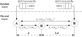
Figure 1: Cross-layer two-way relay model.

III-B Channel Model

We consider the scenario in which all nodes have perfect channel state information. The channel coefficients of all links are assumed to remain unchanged within each time frame but vary from one frame to another. The instantaneous channel coefficient between node $i$ and $j$ is denoted as $h_{i,j}$, where $i,j\in\{A,B,R\}$ with $i\neq j$. Here the channel reciprocity is assumed, i.e., $h_{i,j}=h_{j,i}$, which is valid in time-division duplex mode. Without loss of generality, it is assumed that the additive noises at all nodes are independent circularly symmetric complex Gaussian random variables, each having zero mean and unit variance. For notational convenience, we further define the instantaneous network channel state information as a three-tuple $\boldsymbol{\gamma}=(\gamma_{1},\gamma_{2},\gamma_{3})$, where $\gamma_{1}=|h_{A,R}|^{2},\gamma_{2}=|h_{B,R}|^{2},\gamma_{3}=|h_{A,B}|^{2}$ (as shown in Fig. 1).

III-C Two-Way Relay Protocols

Different two-way relay protocols have been studied in the literature [3, 4, 5, 6, 9]. In this paper, we focus on the three-phase and two-phase two-way relay protocols with DF strategy. Let $P_{A}$, $P_{B}$, and $P_{R}$ denote the transmit power of nodes $A$, $B$, and $R$, respectively. Let $R_{A}$ and $R_{B}$ denote the achievable rates from node $A$ to node $B$ and from node $B$ to node $A$, respectively. We further denote $\boldsymbol{P}=[P_{A},P_{B},P_{R}]^{T}$ as the transmit power vector, and $\boldsymbol{R}=[R_{A},R_{B}]^{T}$ as the bidirectional rate pair.

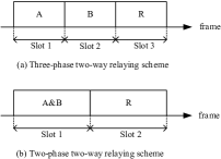
Figure 2: Two-way relay transmission schemes.

III-C1 Three-Phase Two-Way Relaying

In this protocol, the information exchange between A and B is completed in three time slots. As shown in Fig. 2(a), in the first time slot, source node $A$ transmits, while source node $B$ and relay node $R$ listen. In the second time slot, node $B$ transmits, while $A$ and $R$ listen. In the third time slot, the relay node transmits and both $A$ and $B$ listen. Ideally, the time fraction of each slot in every transmission frame can be optimized. In this work we only consider equal time assignment for simplicity, and so is for the two-phase protocol.

The achievable rate region of the three-phase protocol with DF strategy under a given transmit power vector $\boldsymbol{P}$ and network CSI $\boldsymbol{\gamma}$ is [5]

$$\mathcal{R}(\boldsymbol{P},\boldsymbol{\gamma})=\{(R_{A},R_{B})\},$$ (6)

where

$$R_{A}\leq \frac{1}{3}\min\big{\{}C(\gamma_{1}P_{A}),C(\gamma_{3}P_{A})+C(\gamma_{2}P_{R})\big{\}}, \gamma_{1}>\gamma_{3}$$  (7)

$$R_{A}\leq \frac{1}{3}C(\gamma_{3}P_{A}), {\rm otherwise}$$  (8)

$$R_{B}\leq \frac{1}{3}\min\big{\{}C(\gamma_{2}P_{B}),C(\gamma_{3}P_{B})+C(\gamma_{1}P_{R})\big{\}}, \gamma_{2}>\gamma_{3}$$  (9)

$$R_{B}\leq \frac{1}{3}C(\gamma_{3}P_{B}), {\rm otherwise}$$  (10)

with $C(x)=\log_{2}(1+x)$. It shows that if the channel quality of the relay link for one data flow ($\gamma_{1}$ or $\gamma_{2}$) is worse than that of the direct link ($\gamma_{3}$), then direct transmission will be triggered for that flow.

III-C2 Two-Phase Two-Way Relaying

In this scheme, it takes two slots to finish one round of information exchange between the two source nodes. As shown in Fig. 2(b), in the first time slot, which is termed as multiple access (MAC) phase, the nodes $A$ and $B$ simultaneously transmit signals to the relay node $R$. Due to the half-duplex constraint, there is no direct link between nodes $A$ and $B$. In the second time slot, which is known as broadcast (BC) phase, the relay node broadcasts signals to both $A$ and $B$.

The achievable rate region of the two-phase two-way relaying with DF strategy under a given transmit power vector $\boldsymbol{P}$ and network CSI $\boldsymbol{\gamma}$ is [3, 4, 5]

$$\mathcal{R}(\boldsymbol{P},\boldsymbol{\gamma})=\mathcal{C}_{MAC}(P_{A},P_{B},\boldsymbol{\gamma})\cap\mathcal{C}_{BC}(P_{R},\boldsymbol{\gamma}),$$ (11)

where $\mathcal{C}_{MAC}$ and $\mathcal{C}_{BC}$ are the achievable rate regions of the MAC and BC phases, respectively, and can be given by

$$\mathcal{C}_{MAC}(P_{A},P_{B},\boldsymbol{\gamma})=\{(R_{A},R_{B}):R_{A}\leq\frac{1}{2}C(\gamma_{1}P_{A}),$$

$$R_{B}\leq\frac{1}{2}C(\gamma_{2}P_{B}),R_{A}+R_{B}\leq\frac{1}{2}C(\gamma_{1}P_{A}+\gamma_{2}P_{B})\},$$ (12)

$$\mathcal{C}_{BC}(P_{R},\boldsymbol{\gamma})=\{(R_{A},R_{B}): R_{A}\leq\frac{1}{2}C(\gamma_{2}P_{R}),$$ (13)

$$R_{B}\leq\frac{1}{2}C(\gamma_{1}P_{R})\}.$$

Note that both $\mathcal{C}_{MAC}$ and $\mathcal{C}_{BC}$ are convex sets, so is their intersection.

III-D Problem Formulation

In this paper, our objective is to find the optimal transmission policies to maximize the weighted sum rate of the two-way relay system while satisfying the individual delay requirement at each node. As stated before, the effective capacity can be viewed as the maximum throughput under the constraint of QoS exponent in steady state. Hence, we can formulate an equivalent problem, which is to maximize the weighted sum effective capacity for given delay constraints of node $A$ and node $B$, i.e., $\theta_{A}$ and $\theta_{B}$. Our resource allocation policies are based on cross-layer parameters, specifically, the instantaneous network CSI $\boldsymbol{\gamma}=(\gamma_{1},\gamma_{2},\gamma_{3})$ and the delay-QoS requirements $\boldsymbol{\theta}=(\theta_{A},\theta_{B})$. Correspondingly, we define $\boldsymbol{\epsilon}\triangleq(\boldsymbol{\gamma},\boldsymbol{\theta})$. Therefore, the problem can be formulated as follows,

$$\textbf{P1}: \max_{\boldsymbol{P}(\boldsymbol{\epsilon}),\boldsymbol{R}(\boldsymbol{\epsilon})}~{}-\frac{\omega_{A}}{\theta_{A}}\ln\big{(}\mathbb{E}_{\boldsymbol{\gamma}}[e^{-\theta_{A}R_{A}(\boldsymbol{\epsilon})}]\big{)}$$ (19)

$$~{}~{}~{}~{}~{}~{}~{}~{}~{}~{}~{}~{}-\frac{\omega_{B}}{\theta_{B}}\ln\big{(}\mathbb{E}_{\gamma}[e^{-\theta_{B}R_{B}(\boldsymbol{\epsilon})}]\big{)}$$

$$~{}~{}~{}s.t.~{}~{}~{}~{}~{}~{}\mathbb{E}_{\boldsymbol{\gamma}}[P_{A}]\leq\overline{P_{A}}$$

$$~{}~{}~{}~{}~{}~{}~{}~{}~{}~{}~{}~{}~{}\mathbb{E}_{\boldsymbol{\gamma}}[P_{B}]\leq\overline{P_{B}}$$

$$~{}~{}~{}~{}~{}~{}~{}~{}~{}~{}~{}~{}~{}\mathbb{E}_{\boldsymbol{\gamma}}[P_{R}]\leq\overline{P_{R}}$$

$$~{}~{}~{}~{}~{}~{}~{}~{}~{}~{}~{}~{}~{}\boldsymbol{R}(\boldsymbol{\epsilon})\in\mathcal{R}(\boldsymbol{P}(\boldsymbol{\epsilon}),\boldsymbol{\gamma})$$

$$~{}~{}~{}~{}~{}~{}~{}~{}~{}~{}~{}~{}~{}\boldsymbol{P}(\boldsymbol{\epsilon})\succeq 0,$$

where $\omega_{A},\omega_{B}$ are the weights assigned to the two users, satisfying $\omega_{A}+\omega_{B}=1$, and $\overline{P_{A}},\overline{P_{B}},\overline{P_{R}}$ are the long-term power constraints of node $A$, $B$ and $R$, respectively. $\mathbb{E}_{\boldsymbol{\gamma}}[\cdot]$ emphasizes that the expectation is with regard to $\boldsymbol{\gamma}$. $\boldsymbol{P}(\boldsymbol{\epsilon})$ and $\boldsymbol{R}(\boldsymbol{\epsilon})$ denote the power and rate adaptation policies to be optimized, which are functions of $\boldsymbol{\epsilon}$. The instantaneous rate region $\mathcal{R}(\boldsymbol{P}(\boldsymbol{\epsilon}),\boldsymbol{\gamma})$ is defined in (6) for the three-phase protocol, or in (11) for the two-phase protocol. Note that $\mathcal{R}(\boldsymbol{P}(\boldsymbol{\epsilon}),\boldsymbol{\gamma})$ is a convex space spanned by the power sets $\boldsymbol{P}(\boldsymbol{\epsilon})$.

It is proved in [23] that the weighted sum effective capacity is a concave function of the powers in multiuser systems with direct transmission. Using the similar method, we can prove the weighted sum effective capacity in the two-way relay system as given in (19) is also concave of $\boldsymbol{P}(\boldsymbol{\epsilon})$. The main reason is that the achievable rate pair $R_{A}$ and $R_{B}$ are both concave with respect to the power vector $\boldsymbol{P}$. In addition, the power constraints (19)-(19) and (19) are affine. Thus, the problem P1 is a convex optimization problem, and there exists a unique and optimal solution. In the next two sections, we shall develop the optimal power and rate adaptation policies of the given problem for the three-phase and two-phase protocols, respectively.

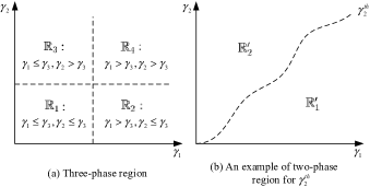
Figure 3: Cross-layer two-way relaying channel state region.

IV Optimal Policy for Three-Phase Two-way Relaying

In this section, we first derive the optimal transmission policy for the three-phase two-way relaying subject to general delay QoS requirements $\boldsymbol{\theta}=(\theta_{A},\theta_{B})$, for which $\mathcal{R}(\boldsymbol{P}(\boldsymbol{\epsilon}),\boldsymbol{\gamma})$ is given in (6). Then we consider the limiting case when both $\theta_{A}$ and $\theta_{B}$ approach zero, i.e., the ergodic capacity problem.

IV-A Optimal Policy

We define the Lagrangian of problem P1 as

$$\mathcal{L}\big{(}\boldsymbol{P}(\boldsymbol{\epsilon}),\boldsymbol{R}(\boldsymbol{\epsilon}),\boldsymbol{\lambda}\big{)}$$ (20)

$$= -\frac{\omega_{A}}{\theta_{A}}\ln\big{(}\mathbb{E}_{\boldsymbol{\gamma}}[e^{-\theta_{A}R_{A}(\boldsymbol{\epsilon})}]\big{)}-\frac{\omega_{B}}{\theta_{B}}\ln\big{(}\mathbb{E}_{\gamma}[e^{-\theta_{B}R_{B}(\boldsymbol{\epsilon})}]\big{)}$$

$$+\lambda_{A}\big{(}\overline{P_{A}}-\mathbb{E}_{\boldsymbol{\gamma}}[P_{A}(\boldsymbol{\epsilon})]\big{)}+\lambda_{B}\big{(}\overline{P_{B}}-\mathbb{E}_{\boldsymbol{\gamma}}[P_{B}(\boldsymbol{\epsilon})]\big{)}$$

$$+\lambda_{R}\big{(}\overline{P_{R}}-\mathbb{E}_{\boldsymbol{\gamma}}[P_{R}(\boldsymbol{\epsilon})]\big{)},$$

where $\boldsymbol{\lambda}=[\lambda_{A},\lambda_{B},\lambda_{R}]^{T}$ are the Lagrange multipliers related to the power constraints (19)-(19). Then the dual problem of P1 can be stated as

$$\textbf{P2}:~{} \min_{\boldsymbol{\lambda}\geq 0}~{}\max_{\begin{subarray}{c}\boldsymbol{P}(\boldsymbol{\epsilon})\succeq 0,\\ \boldsymbol{R}(\boldsymbol{\epsilon})\in\mathcal{R}\end{subarray}}~{}\mathcal{L}\big{(}\boldsymbol{P}(\boldsymbol{\epsilon}),\boldsymbol{R}(\boldsymbol{\epsilon}),\boldsymbol{\lambda}\big{)}.$$

Note that the subgradient method can be used to update $\boldsymbol{\lambda}$ toward the optimal $\boldsymbol{\lambda}^{*}$ as follows

$$\boldsymbol{\lambda}^{(i+1)}=\boldsymbol{\lambda}^{(i)}-\boldsymbol{s}^{(i)}\big{(}\boldsymbol{\overline{P}}-\mathbb{E}_{\boldsymbol{\gamma}}[\boldsymbol{P}(\boldsymbol{\epsilon})]\big{)},$$ (21)

where the subscript $i$ denotes the iteration index, and $\boldsymbol{s}^{(i)}$ is the vector of step size designed properly.

According to the achievable rate region defined in (6), we divide the channel states $\boldsymbol{\gamma}$ into four regions as shown in Fig. 3(a). In the following, we provide the optimal transmission policy for each channel region, and the detailed derivations are given in Appendix A.

IV-A1 Region $\mathbb{R}_{1}(\gamma_{1}\leq\gamma_{3},\gamma_{2}\leq\gamma_{3})$

In this case, the achievable rate pair $R_{A}$ and $R_{B}$ satisfy (8) and (10), respectively, which means that the bidirectional links follow direct transmission. It is obvious that the optimal rates are exactly the capacity bound, given by

$$R_{A}(\boldsymbol{\epsilon})=\frac{1}{3}C\big{(}\gamma_{3}P_{A}(\boldsymbol{\epsilon})\big{)},$$ (22)

$$R_{B}(\boldsymbol{\epsilon})=\frac{1}{3}C\big{(}\gamma_{3}P_{B}(\boldsymbol{\epsilon})\big{)}.$$ (23)

Substituting the above into the Lagrangian function (20) to eliminate the rate variables, we can then obtain the closed-form expressions of the optimal power allocation as

$$\begin{cases}P_{A}(\boldsymbol{\epsilon})=\bigg{[}\bigg{(}\frac{\sigma\lambda_{A}\phi_{1}}{\omega_{A}}\bigg{)}^{-\frac{3}{\beta_{A}+3}}\gamma_{3}^{-\frac{\beta_{A}}{\beta_{A}+3}}-\gamma_{3}^{-1}\bigg{]}^{+}\\ P_{B}(\boldsymbol{\epsilon})=\bigg{[}\bigg{(}\frac{\sigma\lambda_{B}\phi_{2}}{\omega_{B}}\bigg{)}^{-\frac{3}{\beta_{B}+3}}\gamma_{3}^{-\frac{\beta_{B}}{\beta_{B}+3}}-\gamma_{3}^{-1}\bigg{]}^{+}\\ P_{R}(\boldsymbol{\epsilon})=0,\end{cases}$$ (24)

where $\sigma=3\ln 2$, $\beta_{i}=\frac{\theta_{i}}{\ln 2},i\in\{A,B\}$, and

$$\phi_{1}=\mathbb{E}_{\boldsymbol{\gamma}}\big{[}e^{-\theta_{A}R_{A}(\boldsymbol{\epsilon})}\big{]},$$ (25)

$$\phi_{2}=\mathbb{E}_{\boldsymbol{\gamma}}\big{[}e^{-\theta_{B}R_{B}(\boldsymbol{\epsilon})}\big{]}.$$ (26)

Note that $\phi_{1}$, $\phi_{2}$ are expectations over all the regions, and should be updated with $\boldsymbol{\lambda}$ in each iteration of the dual problem.

IV-A2 Region $\mathbb{R}_{2}(\gamma_{1}>\gamma_{3},\gamma_{2}\leq\gamma_{3})$

In this region, node $A$ transmits signals with the help of node $R$ while node $B$ adopts direct transmission. According to (7) and (10), the optimal rate allocation is given by

$$R_{A}(\boldsymbol{\epsilon})=\frac{1}{3}\min\big{\{}C\big{(}\gamma_{1}P_{A}(\boldsymbol{\epsilon})\big{)},C\big{(}\gamma_{3}P_{A}(\boldsymbol{\epsilon})\big{)}+C\big{(}\gamma_{2}P_{R}(\boldsymbol{\epsilon})\big{)}\big{\}},$$ (27)

$$R_{B}(\boldsymbol{\epsilon})=\frac{1}{3}C\big{(}\gamma_{3}P_{B}(\boldsymbol{\epsilon})\big{)}.$$ (28)

Then the optimal power allocation can be obtained as

$$\begin{cases}P_{A}(\boldsymbol{\epsilon})=\big{[}\widehat{P}_{A}(\boldsymbol{\epsilon})\big{]}^{+}\\ P_{B}(\boldsymbol{\epsilon})=\bigg{[}\bigg{(}\frac{\sigma\lambda_{B}\phi_{2}}{\omega_{B}}\bigg{)}^{-\frac{3}{\beta_{B}+3}}\gamma_{3}^{-\frac{\beta_{B}}{\beta_{B}+3}}-\gamma_{3}^{-1}\bigg{]}^{+}\\ P_{R}(\boldsymbol{\epsilon})=\frac{(\gamma_{1}-\gamma_{3})P_{A}(\boldsymbol{\epsilon})}{\gamma_{2}[1+\gamma_{3}P_{A}(\boldsymbol{\epsilon})]},\end{cases}$$ (29)

where $\widehat{P}_{A}(\boldsymbol{\epsilon})$ is the solution of the following equation

$$\frac{\omega_{A}\gamma_{1}}{\sigma\phi_{1}}\big{[}1+\gamma_{1}\widehat{P}_{A}(\boldsymbol{\epsilon})\big{]}^{-\frac{\beta_{A}+3}{3}}-\frac{\lambda_{R}(\gamma_{1}-\gamma_{3})}{\gamma_{2}\big{[}1+\gamma_{3}\widehat{P}_{A}(\boldsymbol{\epsilon})\big{]}^{2}}-\lambda_{A}=0.$$ (30)

We use the simple bisection method to obtain $\widehat{P}_{A}(\boldsymbol{\epsilon})$ since (30) is a monotonically decreasing function of $\widehat{P}_{A}(\boldsymbol{\epsilon})$.

IV-A3 Region $\mathbb{R}_{3}(\gamma_{1}\leq\gamma_{3},\gamma_{2}>\gamma_{3})$

Node $B$ transmits signals via the assistance of the relay while node $A$ adopts direct transmission. This case is similar to that of $\mathbb{R}_{2}$ and we omit the results here.

IV-A4 Region $\mathbb{R}_{4}(\gamma_{1}>\gamma_{3},\gamma_{2}>\gamma_{3})$

In this region, both source nodes need the relay node’s help. According to the achievable rate pair (7) and (9), the optimal rate should follow

$$R_{A}(\boldsymbol{\epsilon})=\frac{1}{3}\min\big{\{}C\big{(}\gamma_{1}P_{A}(\boldsymbol{\epsilon})\big{)},C\big{(}\gamma_{3}P_{A}(\boldsymbol{\epsilon})\big{)}+C\big{(}\gamma_{2}P_{R}(\boldsymbol{\epsilon})\big{)}\big{\}},$$ (31)

$$R_{B}(\boldsymbol{\epsilon})=\frac{1}{3}\min\big{\{}C\big{(}\gamma_{2}P_{B}(\boldsymbol{\epsilon})\big{)},C\big{(}\gamma_{3}P_{B}(\boldsymbol{\epsilon})\big{)}+C\big{(}\gamma_{1}P_{R}(\boldsymbol{\epsilon})\big{)}\big{\}}.$$ (32)

The associated optimal power allocation is as follows. Define

$$\tau\triangleq\frac{\gamma_{1}(\gamma_{1}-\gamma_{3})}{\gamma_{2}(\gamma_{2}-\gamma_{3})}.$$ (33)

If $\tau\leq 1$, i.e., $\gamma_{3}<\gamma_{1}\leq\gamma_{2}$, we have

$$\begin{cases}P_{A}(\boldsymbol{\epsilon})=\big{[}\widehat{P}_{A}(\boldsymbol{\epsilon})\big{]}^{+}\\ P_{B}(\boldsymbol{\epsilon})=\frac{\tau P_{A}(\boldsymbol{\epsilon})}{1+(1-\tau)\gamma_{3}P_{A}(\boldsymbol{\epsilon})}\\ P_{R}(\boldsymbol{\epsilon})=\frac{(\gamma_{1}-\gamma_{3})P_{A}(\boldsymbol{\epsilon})}{\gamma_{2}[1+\gamma_{3}P_{A}(\boldsymbol{\epsilon})]},\\ \end{cases}$$ (34)

where $\widehat{P}_{A}(\boldsymbol{\epsilon})$ is the solution of

$$\frac{\omega_{A}\gamma_{1}}{\sigma\phi_{1}}\big{[}1+\gamma_{1}\widehat{P}_{A}(\boldsymbol{\epsilon})\big{]}^{-\frac{\beta_{A}+3}{3}}+\frac{\tau\omega_{B}\gamma_{2}}{\sigma\phi_{2}\big{[}1+(1-\tau)\gamma_{3}\widehat{P}_{A}(\boldsymbol{\epsilon})\big{]}^{2}}$$

$$\times\bigg{[}1+\frac{\tau\gamma_{2}\widehat{P}_{A}(\boldsymbol{\epsilon})}{1+(1-\tau)\gamma_{3}\widehat{P}_{A}(\boldsymbol{\epsilon})}\bigg{]}^{-\frac{\beta_{B}+3}{3}}-\frac{\lambda_{R}(\gamma_{1}-\gamma_{3})}{\gamma_{2}\big{[}1+\gamma_{3}\widehat{P}_{A}(\boldsymbol{\epsilon})\big{]}^{2}}$$

$$-\frac{\tau\lambda_{B}}{\big{[}1+(1-\tau)\gamma_{3}\widehat{P}_{A}(\boldsymbol{\epsilon})\big{]}^{2}}-\lambda_{A}=0.$$ (35)

Note that the bisection method can be used to obtain $\widehat{P}_{A}(\boldsymbol{\epsilon})$ since (IV-A4) is a monotonically decreasing function of $\widehat{P}_{A}(\boldsymbol{\epsilon})$.

If $\tau>1$, i.e., $\gamma_{3}<\gamma_{2}<\gamma_{1}$, we have

$$\begin{cases}P_{A}(\boldsymbol{\epsilon})=\frac{P_{B}(\boldsymbol{\epsilon})}{\tau+(\tau-1)\gamma_{3}P_{B}(\boldsymbol{\epsilon})}\\ P_{B}(\boldsymbol{\epsilon})=\big{[}\widehat{P}_{B}(\boldsymbol{\epsilon})\big{]}^{+}\\ P_{R}(\boldsymbol{\epsilon})=\frac{(\gamma_{2}-\gamma_{3})P_{B}(\boldsymbol{\epsilon})}{\gamma_{1}[1+\gamma_{3}P_{B}(\boldsymbol{\epsilon})]},\\ \end{cases}$$ (36)

where $\widehat{P}_{B}(\boldsymbol{\epsilon})$ is the solution of

$$\frac{\omega_{B}\gamma_{2}}{\sigma\phi_{2}}\big{[}1+\gamma_{2}\widehat{P}_{B}(\boldsymbol{\epsilon})\big{]}^{-\frac{\beta_{B}+3}{3}}+\frac{\tau\omega_{A}\gamma_{1}}{\sigma\phi_{1}\big{[}\tau+(\tau-1)\gamma_{3}\widehat{P}_{B}(\boldsymbol{\epsilon})\big{]}^{2}}$$

$$\times\bigg{[}1+\frac{\gamma_{1}\widehat{P}_{B}(\boldsymbol{\epsilon})}{\tau+(\tau-1)\gamma_{3}\widehat{P}_{B}(\boldsymbol{\epsilon})}\bigg{]}^{-\frac{\beta_{A}+3}{3}}-\frac{\lambda_{R}(\gamma_{2}-\gamma_{3})}{\gamma_{1}\big{[}1+\gamma_{3}\widehat{P}_{B}(\boldsymbol{\epsilon})\big{]}^{2}}$$

$$-\frac{\tau\lambda_{A}}{\big{[}\tau+(\tau-1)\gamma_{3}\widehat{P}_{B}(\boldsymbol{\epsilon})\big{]}^{2}}-\lambda_{B}=0,$$ (37)

which can also be obtained by the bisection method as (IV-A4).

In summary, the optimal transmission policy $\{\boldsymbol{P}(\boldsymbol{\epsilon}),\boldsymbol{R}(\boldsymbol{\epsilon})\}$ for the three-phase two-way relaying is given by (24), (22), (23) when $\gamma_{1}\leq\gamma_{3},\gamma_{2}\leq\gamma_{3}$, by (29), (27), (28) when $\gamma_{1}>\gamma_{3},\gamma_{2}\leq\gamma_{3}$, by (34), (31), (32) when $\gamma_{3}<\gamma_{1}\leq\gamma_{2}$, and by (36), (31), (32) when $\gamma_{3}<\gamma_{2}<\gamma_{1}$. The detailed derivations are given in Appendix A.

IV-B A Special Case

As reviewed in Section II-A, the dynamics of $\theta$ correspond to diverse delay-QoS requirements. In particular, in our two-way relay system model, if $\theta_{A}=\theta_{B}\rightarrow 0$, meaning the services of the two nodes are non-real-time, then the weighted sum of effective capacity yields the weighted ergodic capacity.

Letting $\theta_{A}=\theta_{B}\rightarrow 0$ in (24), (29), (34) and (36), we can obtain the optimal transmission policy for weighted ergodic capacity maximization. For example, in region $\mathbb{R}_{1}$, the optimal powers are given by

$$\begin{cases}P_{A}^{*}(\boldsymbol{\epsilon})=\bigg{[}\bigg{(}\frac{\sigma\lambda_{A}}{\omega_{A}}\bigg{)}^{-1}-\gamma_{3}^{-1}\bigg{]}^{+}\\ P_{B}^{*}(\boldsymbol{\epsilon})=\bigg{[}\bigg{(}\frac{\sigma\lambda_{B}}{\omega_{B}}\bigg{)}^{-1}-\gamma_{3}^{-1}\bigg{]}^{+}\\ P_{R}^{*}(\boldsymbol{\epsilon})=0,\end{cases}$$ (38)

which have the standard form of water-filling. For the rest three regions, similar results can be obtained.

V Optimal Policy for Two-Phase Two-way Relaying

In this section, in accord with $\mathcal{R}(\boldsymbol{P}(\boldsymbol{\epsilon}),\boldsymbol{\gamma})$ given in (11), we present the optimal transmission policy for the two-phase two-way relaying, as well as the optimal partition criterion in the MAC phase. Meanwhile, the problem in limiting case when $\theta_{A}=\theta_{B}=0$ is also analyzed.

V-A Optimal Policy

The rate constraints in the BC phase of this protocol can be equally rewritten as

$$\frac{1}{\theta_{A}}~{}e^{-\theta_{A}R_{A}(\boldsymbol{\epsilon})}\geq\frac{1}{\theta_{A}}~{}e^{-\frac{\theta_{A}}{2}C(\gamma_{2}P_{R}(\boldsymbol{\epsilon}))},$$ (39)

$$\frac{1}{\theta_{B}}~{}e^{-\theta_{B}R_{B}(\boldsymbol{\epsilon})}\geq\frac{1}{\theta_{B}}~{}e^{-\frac{\theta_{B}}{2}C(\gamma_{1}P_{R}(\boldsymbol{\epsilon}))}.$$ (40)

By using the Lagrange dual method [29], we can involve the two rate constraints into the objective function of P1. Then, the resulting Lagrangian can be expressed as

$$\mathscr{L}\big{(}\boldsymbol{P}(\boldsymbol{\epsilon}),\boldsymbol{R}(\boldsymbol{\epsilon}),\boldsymbol{\lambda},\boldsymbol{\mu}\big{)}$$ (41)

$$= -\frac{\omega_{A}}{\theta_{A}}\ln\big{(}\mathbb{E}_{\boldsymbol{\gamma}}[e^{-\theta_{A}R_{A}(\boldsymbol{\epsilon})}]\big{)}-\frac{\omega_{B}}{\theta_{B}}\ln\big{(}\mathbb{E}_{\gamma}[e^{-\theta_{B}R_{B}(\boldsymbol{\epsilon})}]\big{)}$$

$$+\mathbb{E}_{\boldsymbol{\gamma}}\left[\frac{\mu_{A}}{\theta_{A}}\bigg{(}e^{-\theta_{A}R_{A}(\boldsymbol{\epsilon})}-e^{-\frac{\theta_{A}}{2}C(\gamma_{2}P_{R}(\boldsymbol{\epsilon}))}\bigg{)}\right]$$

$$+\mathbb{E}_{\boldsymbol{\gamma}}\left[\frac{\mu_{B}}{\theta_{B}}\bigg{(}e^{-\theta_{B}R_{B}(\boldsymbol{\epsilon})}-e^{-\frac{\theta_{B}}{2}C(\gamma_{1}P_{R}(\boldsymbol{\epsilon}))}\bigg{)}\right]$$

$$+\lambda_{A}\big{(}\overline{P_{A}}-\mathbb{E}_{\boldsymbol{\gamma}}[P_{A}(\boldsymbol{\epsilon})]\big{)}+\lambda_{B}\big{(}\overline{P_{B}}-\mathbb{E}_{\boldsymbol{\gamma}}[P_{B}(\boldsymbol{\epsilon})]\big{)}$$

$$+\lambda_{R}\big{(}\overline{P_{R}}-\mathbb{E}_{\boldsymbol{\gamma}}[P_{R}(\boldsymbol{\epsilon})]\big{)},$$

where $\boldsymbol{\mu}=[\mu_{A},\mu_{B}]^{T}$ are the Lagrange multipliers associated with the rate constraints on $R_{A}(\boldsymbol{\epsilon})$ and $R_{B}(\boldsymbol{\epsilon})$ in (39), (40), $\boldsymbol{\lambda}=[\lambda_{A},\lambda_{B},\lambda_{R}]^{T}$ are the Lagrange multipliers related to the power constraints. As a result, the dual problem can be stated as

$$\textbf{P3}:~{} \min_{\boldsymbol{\lambda}\succeq 0,\boldsymbol{\mu}\succeq 0}~{}\max_{\begin{subarray}{c}\boldsymbol{P}(\boldsymbol{\epsilon})\succeq 0,\\ \boldsymbol{R}(\boldsymbol{\epsilon})\in\mathcal{C}_{MAC}\end{subarray}}~{}\mathscr{L}\big{(}\boldsymbol{P}(\boldsymbol{\epsilon}),\boldsymbol{R}(\boldsymbol{\epsilon}),\boldsymbol{\lambda},\boldsymbol{\mu}\big{)}.$$

Taking a close look at the above dual function, we find that the optimization of the relay power policy $P_{R}(\boldsymbol{\epsilon})$ can be decoupled from others. Therefore, the dual function can be computed by solving the two subproblems as follows,

$${\rm subproblem~{}1}:$$ (43)

$$\max_{\begin{subarray}{c}P_{A}(\boldsymbol{\epsilon})\geq 0,\\ P_{B}(\boldsymbol{\epsilon})\geq 0,\\ R_{A}(\boldsymbol{\epsilon}),R_{B}(\boldsymbol{\epsilon})\end{subarray}}~{}-\frac{\omega_{A}}{\theta_{A}}\ln\big{(}\mathbb{E}_{\boldsymbol{\gamma}}[e^{-\theta_{A}R_{A}(\boldsymbol{\epsilon})}]\big{)}$$

$$-\frac{\omega_{B}}{\theta_{B}}\ln\big{(}\mathbb{E}_{\gamma}[e^{-\theta_{B}R_{B}(\boldsymbol{\epsilon})}]\big{)}$$

$$+\mathbb{E}_{\boldsymbol{\gamma}}\left[\frac{\mu_{A}}{\theta_{A}}e^{-\theta_{A}R_{A}(\boldsymbol{\epsilon})}\right]+\mathbb{E}_{\boldsymbol{\gamma}}\left[\frac{\mu_{B}}{\theta_{B}}e^{-\theta_{B}R_{B}(\boldsymbol{\epsilon})}\right]$$

$$+\lambda_{A}\big{(}\overline{P_{A}}-\mathbb{E}_{\boldsymbol{\gamma}}[P_{A}(\boldsymbol{\epsilon})]\big{)}$$

$$+\lambda_{B}\big{(}\overline{P_{B}}-\mathbb{E}_{\boldsymbol{\gamma}}[P_{B}(\boldsymbol{\epsilon})]\big{)}$$

$$~{}~{}~{}~{}s.t.~{}~{}~{}~{}~{}~{}\big{(}R_{A}(\boldsymbol{\epsilon}),R_{B}(\boldsymbol{\epsilon})\big{)}\in\mathcal{C}_{MAC}\big{(}P_{A}(\boldsymbol{\epsilon}),P_{B}(\boldsymbol{\epsilon}),\boldsymbol{\gamma}\big{)},$$

and

$${\rm subproblem~{}2}:$$

$$\max_{P_{R}(\boldsymbol{\epsilon})\geq 0}~{}-\mathbb{E}_{\boldsymbol{\gamma}}\bigg{[}\frac{\mu_{A}}{\theta_{A}}\big{(}1+\gamma_{2}P_{R}(\boldsymbol{\epsilon})\big{)}^{-\frac{\beta_{A}}{2}}\bigg{]}$$

$$~{}~{}~{}~{}~{}~{}~{}~{}~{}~{}-\mathbb{E}_{\boldsymbol{\gamma}}\bigg{[}\frac{\mu_{B}}{\theta_{B}}\big{(}1+\gamma_{1}P_{R}(\boldsymbol{\epsilon})\big{)}^{-\frac{\beta_{B}}{2}}\bigg{]}$$

$$~{}~{}~{}~{}~{}~{}~{}~{}~{}~{}+\lambda_{R}\big{(}\overline{P_{R}}-\mathbb{E}_{\boldsymbol{\gamma}}[P_{R}(\boldsymbol{\epsilon})]\big{)},$$ (44)

where $\beta_{i}=\frac{\theta_{i}}{\ln 2},i\in\{A,B\}$, is the same as the definition in Section IV-A. Then the dual problem P3 can be solved through two nested dual searching loops. The inner loop searches $\boldsymbol{\mu}$ for given $\boldsymbol{\lambda}$ and the outer loop searches $\boldsymbol{\lambda}$ for given $\boldsymbol{\mu}$, where the values $\boldsymbol{\mu}$ and $\boldsymbol{\lambda}$ can be updated iteratively using the subgradient method with guaranteed convergence as

$$\mu_{A}^{(i+1)}=\mu_{A}^{(i)}-z_{A}^{(i)}\left(e^{-\theta_{A}R_{A}(\boldsymbol{\epsilon})}-e^{-\frac{\theta_{A}}{2}C(\gamma_{2}P_{R}(\boldsymbol{\epsilon}))}\right),$$ (45)

$$\mu_{B}^{(i+1)}=\mu_{B}^{(i)}-z_{B}^{(i)}\left(e^{-\theta_{B}R_{B}(\boldsymbol{\epsilon})}-e^{-\frac{\theta_{B}}{2}C(\gamma_{1}P_{R}(\boldsymbol{\epsilon}))}\right),$$ (46)

$$\boldsymbol{\lambda}^{(i+1)}=\boldsymbol{\lambda}^{(i)}-\boldsymbol{s}^{(i)}\big{(}\boldsymbol{\overline{P}}-\mathbb{E}_{\boldsymbol{\gamma}}[\boldsymbol{P}(\boldsymbol{\epsilon})]\big{)},$$ (47)

where the subscript $i$ denotes the iteration index, and $z_{A}^{(i)}$, $z_{B}^{(i)}$ and $\boldsymbol{s}^{(i)}$ are the step sizes designed properly. The overall algorithm is specified later. In the following, we solve the two subproblems respectively.

V-A1 Solution of Subproblem 1

The first subproblem is relevant to $P_{A}(\boldsymbol{\epsilon})$ and $P_{B}(\boldsymbol{\epsilon})$ in the MAC phase but not $P_{R}(\boldsymbol{\epsilon})$ in the BC phase. It is essentially a classical resource allocation problem in MAC channels, though the objective function is slightly different from the Gaussian MAC [26]. As shown in [26], successive decoding is the optimal strategy for resource allocation in MAC channels. Motivated by this result, we partition the channel states into two regions, $\mathbb{R}^{\prime}_{1}$ and $\mathbb{R}^{\prime}_{2}$, for which an example is shown in Fig. 3(b). In region $\mathbb{R}^{\prime}_{1}$, the relay first decodes the signal from node $A$, then subtracts this decoded signal from the received signal, and then decodes the signal from node $B$. Inversely, in region $\mathbb{R}^{\prime}_{2}$, the relay decodes the signal from node $B$ first and then the signal from node $A$. Similar partition method is used in the literature (e.g., [27, 28]). In the following, we propose the optimal power and rate adaptation policy for a given channel partition. The optimal channel partition method will be derived in the next subsection.

In region $\mathbb{R}^{\prime}_{1}$, the maximum rates are achieved at [26]

$$R_{A}(\boldsymbol{\epsilon}) = \frac{1}{2}C\bigg{(}\frac{\gamma_{1}P_{A}(\boldsymbol{\epsilon})}{1+\gamma_{2}P_{B}(\boldsymbol{\epsilon})}\bigg{)},$$ (48)

$$R_{B}(\boldsymbol{\epsilon}) = \frac{1}{2}C\big{(}\gamma_{2}P_{B}(\boldsymbol{\epsilon})\big{)},$$ (49)

while in $\mathbb{R}^{\prime}_{2}$, the maximum rates are achieved at

$$R_{A}(\boldsymbol{\epsilon}) = \frac{1}{2}C\big{(}\gamma_{1}P_{A}(\boldsymbol{\epsilon})\big{)},$$ (50)

$$R_{B}(\boldsymbol{\epsilon}) = \frac{1}{2}C\bigg{(}\frac{\gamma_{2}P_{B}(\boldsymbol{\epsilon})}{1+\gamma_{1}P_{A}(\boldsymbol{\epsilon})}\bigg{)}.$$ (51)

By applying the Karush-Kuhn-Tucker (KKT) conditions [29], the optimal power adaptation policy for $P_{A}(\boldsymbol{\epsilon})$ and $P_{B}(\boldsymbol{\epsilon})$ in $\mathbb{R}^{\prime}_{1}$ must satisfy the following conditions (the derivation is provided in Appendix B):

$$\begin{cases}P_{A}(\boldsymbol{\epsilon})=\bigg{[}\alpha_{1}^{-\frac{2}{\beta_{A}+2}}\bigg{(}\frac{1+\gamma_{2}P_{B}(\boldsymbol{\epsilon})}{\gamma_{1}}\bigg{)}^{\frac{\beta_{A}}{\beta_{A}+2}}-\frac{1+\gamma_{2}P_{B}(\boldsymbol{\epsilon})}{\gamma_{1}}\bigg{]}^{+}\\ P_{B}(\boldsymbol{\epsilon})=\big{[}\widehat{P}_{B}(\boldsymbol{\epsilon})\big{]}^{+},\end{cases}$$ (52)

where $\widehat{P}_{B}(\boldsymbol{\epsilon})$ can be obtained using a numerical search through the following equation

$$\frac{\gamma_{2}}{\alpha_{2}}\big{[}1+\gamma_{2}\widehat{P}_{B}(\boldsymbol{\epsilon})\big{]}^{-\frac{\beta_{B}+2}{2}}+\frac{\lambda_{A}\gamma_{2}}{\lambda_{B}\gamma_{1}}$$

$$-\frac{\lambda_{A}\gamma_{2}}{\lambda_{B}\gamma_{1}}\bigg{(}\frac{\alpha_{1}}{\gamma_{1}}\bigg{)}^{-\frac{2}{\beta_{A}+2}}\big{[}1+\gamma_{2}\widehat{P}_{B}(\boldsymbol{\epsilon})\big{]}^{-\frac{2}{\beta_{A}+2}}-1=0,$$ (53)

with

$$\alpha_{1}=\frac{\delta\lambda_{A}}{\omega_{A}{\phi_{1}^{\prime}}^{-1}-\mu_{A}},~{}~{}~{}~{}\alpha_{2}=\frac{\delta\lambda_{B}}{\omega_{B}{\phi_{2}^{\prime}}^{-1}-\mu_{B}},$$

$$\phi^{\prime}_{1} = \int_{\boldsymbol{\gamma}\in\mathbb{R}^{\prime}_{1}}\left[1+\frac{\gamma_{1}P_{A}(\boldsymbol{\epsilon})}{1+\gamma_{2}P_{B}(\boldsymbol{\epsilon})}\right]^{-\frac{\beta_{A}}{2}}\mathit{p}_{\boldsymbol{\gamma}}(\gamma_{1},\gamma_{2})d\gamma_{1}d\gamma_{2}$$

$$+\int_{\boldsymbol{\gamma}\in\mathbb{R}^{\prime}_{2}}\big{[}1+\gamma_{1}P_{A}(\boldsymbol{\epsilon})\big{]}^{-\frac{\beta_{A}}{2}}\mathit{p}_{\boldsymbol{\gamma}}(\gamma_{1},\gamma_{2})d\gamma_{1}d\gamma_{2},$$

$$\phi^{\prime}_{2}=\int_{\boldsymbol{\gamma}\in\mathbb{R}^{\prime}_{1}}\big{[}1+\gamma_{2}P_{B}(\boldsymbol{\epsilon})\big{]}^{-\frac{\beta_{B}}{2}}\mathit{p}_{\boldsymbol{\gamma}}(\gamma_{1},\gamma_{2})d\gamma_{1}d\gamma_{2}$$

$$+\int_{\boldsymbol{\gamma}\in\mathbb{R}^{\prime}_{2}}\left[1+\frac{\gamma_{2}P_{B}(\boldsymbol{\epsilon})}{1+\gamma_{1}P_{A}(\boldsymbol{\epsilon})}\right]^{-\frac{\beta_{B}}{2}}\mathit{p}_{\boldsymbol{\gamma}}(\gamma_{1},\gamma_{2})d\gamma_{1}d\gamma_{2},$$

where $\delta=2\ln 2$. Like the three-phase two-way relaying, $\phi_{1}^{\prime}$ and $\phi_{2}^{\prime}$ are also updated with $\boldsymbol{\lambda}$ in each iteration.

Using the similar method, the optimal power allocation in region $\mathbb{R}^{\prime}_{2}$ can be obtained and the details are omitted.

V-A2 Solution of Subproblem 2

The second subproblem is only relevant to $P_{R}(\boldsymbol{\epsilon})$ in the BC phase, which is also a convex problem. By applying the KKT conditions, we can obtain the optimal power allocation $P_{R}(\boldsymbol{\epsilon})=\big{[}\widehat{P}_{R}(\boldsymbol{\epsilon})\big{]}^{+}$, where $\widehat{P}_{R}(\boldsymbol{\epsilon})$ must satisfy the following equation

$$\mu_{A}\gamma_{2}\big{[}1+\gamma_{2}\widehat{P}_{R}(\boldsymbol{\epsilon})\big{]}^{-\frac{\beta_{A}+2}{2}}$$

$$+\mu_{B}\gamma_{1}\big{[}1+\gamma_{1}\widehat{P}_{R}(\boldsymbol{\epsilon})\big{]}^{-\frac{\beta_{B}+2}{2}}-\delta\lambda_{R}=0.$$ (54)

We apply the bisection method to obtain $\widehat{P}_{R}(\boldsymbol{\epsilon})$ since (V-A2) is a monotonically decreasing function of $\widehat{P}_{R}(\boldsymbol{\epsilon})$.

V-B Optimal Partition Criterion

In the above subsection, we have demonstrated the optimal transmission policy for given decoding region $\mathbb{R}^{\prime}=(\mathbb{R}^{\prime}_{1},\mathbb{R}^{\prime}_{2})$ in the MAC phase. Here we present the optimal partition criterion to determine the decoding order in the MAC phase based on the obtained transmission policy.

To maximize the weighted sum effective capacity in (43), the optimal decoding order in the MAC phase should be dynamic with respect to different channel state information. Similar to [27, 28], finding such optimal partition can be viewed as finding an optimal threshold, $\gamma_{1}^{th}$ for $\gamma_{1}$ or $\gamma_{2}^{th}$ for $\gamma_{2}$. Here $\gamma_{2}^{th}$ (or $\gamma_{1}^{th}$) is a function of both $\gamma_{1}$ (or $\gamma_{2}$) and the power allocation policy $\boldsymbol{P}(\boldsymbol{\epsilon})$. The following proposition is established to find the optimal threshold.

Proposition 1 (Optimal Channel Partition Criterion)

When $\gamma_{2}^{th}$ is used to partition $\mathbb{R}^{\prime}$, $\boldsymbol{\gamma}$ falls into region $\mathbb{R}^{\prime}_{1}$ if $\gamma_{2}<\gamma_{2}^{th}$, otherwise $\boldsymbol{\gamma}$ falls into region $\mathbb{R}^{\prime}_{2}$, where $\gamma_{2}^{th}$ must satisfy

$$\frac{\big{[}1+\frac{\gamma_{1}P_{A}(\boldsymbol{\epsilon})}{1+\gamma_{2}^{th}P_{B}(\boldsymbol{\epsilon})}\big{]}^{-\frac{\beta_{A}}{2}}-\big{[}1+\gamma_{1}P_{A}(\boldsymbol{\epsilon})\big{]}^{-\frac{\beta_{A}}{2}}}{\big{[}1+\frac{\gamma_{2}^{th}P_{B}(\boldsymbol{\epsilon})}{1+\gamma_{1}P_{A}(\boldsymbol{\epsilon})}\big{]}^{-\frac{\beta_{B}}{2}}-\big{[}1+\gamma_{2}^{th}P_{B}(\boldsymbol{\epsilon})\big{]}^{-\frac{\beta_{B}}{2}}}=K.$$ (55)

When $\gamma_{1}^{th}$ is used to partition $\mathbb{R}^{\prime}$, $\boldsymbol{\gamma}$ falls into region $\mathbb{R}^{\prime}_{1}$ if $\gamma_{1}>\gamma_{1}^{th}$, otherwise $\boldsymbol{\gamma}$ falls into region $\mathbb{R}^{\prime}_{2}$, where $\gamma_{1}^{th}$ must satisfy

$$\frac{\big{[}1+\frac{\gamma_{1}^{th}P_{A}(\boldsymbol{\epsilon})}{1+\gamma_{2}P_{B}(\boldsymbol{\epsilon})}\big{]}^{-\frac{\beta_{A}}{2}}-\big{[}1+\gamma_{1}^{th}P_{A}(\boldsymbol{\epsilon})\big{]}^{-\frac{\beta_{A}}{2}}}{\big{[}1+\frac{\gamma_{2}P_{B}(\boldsymbol{\epsilon})}{1+\gamma_{1}^{th}P_{A}(\boldsymbol{\epsilon})}\big{]}^{-\frac{\beta_{B}}{2}}-\big{[}1+\gamma_{2}P_{B}(\boldsymbol{\epsilon})\big{]}^{-\frac{\beta_{B}}{2}}}=K.$$ (56)

In both (55) and (56), $K$ is defined as

$$K\triangleq\frac{\theta_{A}(\omega_{B}{\phi^{\prime}_{2}}^{-1}-\mu_{B})}{\theta_{B}(\omega_{A}{\phi^{\prime}_{1}}^{-1}-\mu_{A})}.$$

Proof:

Please see Appendix C. ∎

Particularly, $\gamma_{1}^{th}$ and $\gamma_{2}^{th}$ should be well-defined in the partition criterion, meaning that they should be positive. However, as we know from (55) and (56), they cannot be both positive in some condition. In this case, the obtained positive one is chosen for the partition.

Finally, we describe the overall algorithm in Algorithm 1 to find the optimal power and rate adaptation policy for the two-phase two-way relay protocol. Note that in Algorithm 1, for a given channel partition we can obtain the optimal power allocation, then the optimal power allocation in turn leads to an optimal channel partition. Due to the convexity of the problem, the global convergence and optimality can be guaranteed.

V-C A Special Case

Similar to the three-phase scheme, when $\theta_{A}=\theta_{B}\rightarrow 0$, we can obtain the optimal transmission policy for the two-phase two-way relaying without delay requirements (i.e., the ergodic capacity).

Proposition 2

The optimal power allocation policy for the two-phase two-way DF relaying for weighted ergodic capacity maximization when $\xi_{A}<\xi_{B}$ is determined by

$$P_{A}^{*}(\boldsymbol{\epsilon})=\bigg{[}\frac{\xi_{A}}{\delta\lambda_{A}}-\frac{\xi_{B}-\xi_{A}}{\delta\gamma_{1}(\frac{\lambda_{B}}{\gamma_{2}}-\frac{\lambda_{A}}{\gamma_{1}})}\bigg{]}^{+},$$ (57)

$$P_{B}^{*}(\boldsymbol{\epsilon})=\bigg{[}\frac{\xi_{B}-\xi_{A}}{\delta\gamma_{2}(\frac{\lambda_{B}}{\gamma_{2}}-\frac{\lambda_{A}}{\gamma_{1}})}-\frac{1}{\gamma_{2}}\bigg{]}^{+},$$ (58)

$$P_{R}^{*}(\boldsymbol{\epsilon})=\begin{cases}0,&\lambda_{R}\geq\frac{\mu_{A}\gamma_{1}+\mu_{B}\gamma_{2}}{\delta}\\ \frac{-c_{2}+\sqrt{{c_{2}^{2}-4c_{1}c_{3}}}}{2c_{1}},&{\rm otherwise}\end{cases}$$ (59)

where $\xi_{A}=\omega_{A}-\mu_{A}$, $\xi_{B}=\omega_{B}-\mu_{B}$, and $c_{1}=\lambda_{R}\gamma_{1}\gamma_{2}$, $c_{2}=\lambda_{R}(\gamma_{1}+\gamma_{2})-\gamma_{1}\gamma_{2}(\mu_{A}+\mu_{B})/\delta$, $c_{3}=\lambda_{R}-(\mu_{A}\gamma_{1}+\mu_{B}\gamma_{2})/\delta$. The results for $\xi_{A}\geq\xi_{B}$ can be easily obtained using the same methods.

Proof:

Letting $\theta_{A}=\theta_{B}\rightarrow 0$ in (52) and (V-A2), we have

$$\begin{cases}P_{A}(\boldsymbol{\epsilon})=\big{[}\frac{\xi_{A}}{\delta\lambda_{A}}-\frac{1+\gamma_{2}P_{B}(\boldsymbol{\epsilon})}{\gamma_{1}}\big{]}^{+}\\ P_{B}(\boldsymbol{\epsilon})=\big{[}\frac{\gamma_{2}(\xi_{B}-\xi_{A})}{\delta(\lambda_{B}\gamma_{1}-\lambda_{A}\gamma_{2})}-\frac{1}{\gamma_{2}}\big{]}^{+}\\ \frac{\mu_{A}\gamma_{2}}{1+\gamma_{2}P_{R}(\boldsymbol{\epsilon})}+\frac{\mu_{B}\gamma_{1}}{1+\gamma_{1}P_{R}(\boldsymbol{\epsilon})}-\delta\lambda_{R}=0.\end{cases}$$

Through simple calculation, we can get the desired results (57), (58) and (59) in $\mathbb{R}^{\prime}_{1}$.

For the segmentation of $(\mathbb{R}^{\prime}_{1},\mathbb{R}^{\prime}_{2})$ in the case of $\theta_{A}=\theta_{B}\rightarrow 0$, by applying the proposed optimal partition criterion, we have

$$K=\frac{\theta_{A}(\omega_{B}-\mu_{B})}{\theta_{B}(\omega_{A}-\mu_{A})}=\frac{\xi_{B}}{\xi_{A}}.$$

Under this condition, (55) becomes

$$\bigg{[}\frac{1+\gamma_{1}P_{A}(\boldsymbol{\epsilon})}{1+\gamma_{2}^{th}P_{B}(\boldsymbol{\epsilon})}\bigg{]}^{-\frac{\beta_{A}}{2}}=K.$$

When $\xi_{B}>\xi_{A}$, meaning that $K>1$, $\gamma_{2}^{th}>0$ is well-defined for partition. As $\theta_{A}\rightarrow 0$, we can find

$$\gamma_{2}^{th}\rightarrow\infty,$$

which implies that $\boldsymbol{\gamma}$ always falls into $\mathbb{R}^{\prime}_{1}$. Hence, the proof completes. Similar analysis can also be done when $0\leq K\leq 1$ by using $\gamma_{1}^{th}$. ∎

Algorithm 1 Finding the optimal transmission policy for two-phase two-way relaying

1:  Given $\omega_{A}$, $\omega_{B}$.

2:  Initialize $P_{A}(\boldsymbol{\epsilon})=\overline{P_{A}}$, $P_{B}(\boldsymbol{\epsilon})=\overline{P_{B}}$.

3:  Initialize $\boldsymbol{\lambda}$.

4:  repeat

5:     Initialize $\boldsymbol{\mu}$ for each $\boldsymbol{\gamma}$.

6:     repeat

7:        Determine the decoding order in the MAC phase according to the optimal partition criterion given in Proposition 1.

8:        if the signal from node $A$ is decoded first, i.e., $\boldsymbol{\gamma}\in\mathbb{R}_{1}^{\prime}$ then

9:           Obtain the two source power allocations $P_{A}(\boldsymbol{\epsilon})$ and $P_{B}(\boldsymbol{\epsilon})$ by using (52).

10:           Obtain the relay power allocation $P_{R}(\boldsymbol{\epsilon})$ by using (V-A2).

11:           Obtain the rate adaptation $\boldsymbol{R}(\boldsymbol{\epsilon})$ as (48), (49).

12:           Update $\boldsymbol{\mu}$ using the subgradient method in (45), (46).

13:        else

14:           $\boldsymbol{\gamma}\in\mathbb{R}_{2}^{\prime}$, adopt similar operations as above except that the rate adaptation is given in (50), (51).

15:        end if

16:     until $\boldsymbol{\mu}$ converges.

17:     Update $\boldsymbol{\lambda}$ using the subgradient method in (47).

18:  until $\boldsymbol{\lambda}$ converges.

VI Numerical Results

In this section, extensive numerical results are provided to illustrate the performance of our proposed cross-layer transmission strategies for the two-way relay systems.

As a benchmark, the conventional two-way channel with direct transmission is considered, for which the optimal transmission policy is obtained from [21]. Besides, to show the advantage of the optimal channel partition in the two-phase two-way relaying, the transmission policy using the static weight-based channel partition, as introduced in [26], is studied. Specifically, in the MAC phase of this scheme, the relay always first decodes the signals from the source with smaller weight, regardless of the CSI variation. The weight-based and the proposed CSI-based schemes with fixed power assignment are also studied to illustrate the significance of channel-aware power adaptation. In these fixed power assignment schemes, the instantaneous power of all transmitting nodes is set to be a constant, while the transmission rates are adaptive with respect to the channel fading.

In our numerical evaluation, the relay is located in a line between the two users. We set the distance between node $A$ and $B$ as $2$. The $A$-$R$ distance and the $B$-$R$ distance are denoted as $d$ and $2-d$, respectively, where $0<d<2$. The log-distance path loss model with small-scale Rayleigh fading is assumed. Hence, the network channel information $\gamma_{1},\gamma_{2},\gamma_{3}$ follow independent exponential distribution with parameter $\lambda_{1}=d^{\nu}$, $\lambda_{2}=(2-d)^{\nu}$, and $\lambda_{3}=2^{\nu}$, respectively, where $\nu$ denotes the path loss exponent. A typical value of $\nu$ lies in the range of $(2,5)$, and it is set as $4$ in our examples. The long-term power constraints of the nodes satisfy $\overline{P_{A}}=\overline{P_{B}}=\overline{P_{R}}+3{\rm dB}$. Throughout this section, the weights are given by $\omega_{A}=0.6$ and $\omega_{B}=0.4$ for illustration purpose.

VI-A Performance of Symmetric Relay for Two Sources

In this subsection, we consider the case when relay is in the middle of the two source nodes, namely, $d=1$. Hence, the channels between the sources and the relay are symmetric.

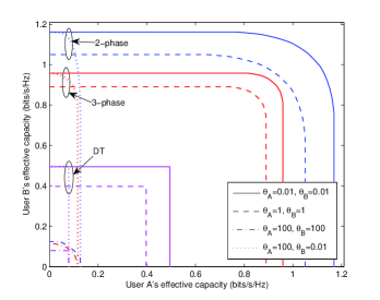
Figure 4: Optimal effective capacity regions for different schemes under diverse delay constraints with $\overline{P_{A}}=\overline{P_{B}}=9{\rm dB},\overline{P_{R}}=6{\rm dB}$.

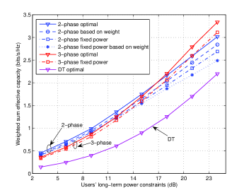
Figure 5: Weighted sum effective capacity versus long-term power constraints under $\theta_{A}=\theta_{B}=1$.

Firstly, in Fig. 4, we plot the optimal effective capacity regions under different delay constraints for the three-phase and two-phase two-way relaying, as well as the two-way direct transmission. We set the long-term power constraints of the source nodes as $9{\rm dB}$. It is observed from Fig. 4 that, with the help of two-way relay, the effective capacity region is significantly expanded compared with the conventional two-way direct transmission. We can also find that, if one user’s delay constraint becomes stringent, its effective capacity becomes small, so is the effective capacity region. This suggests that there is in general a fundamental throughput-delay tradeoff associated with the optimal resource allocation. In addition, under these given power constraints, the effective capacity region of the two-phase protocol is larger than that of the three-phase protocol.

Figure 6: Weighted sum effective capacity versus different delay constraints with long-term power constraints $\overline{P_{A}}=\overline{P_{B}}=9{\rm dB},\overline{P_{R}}=6{\rm dB}$.

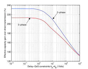
Figure 7: Effective capacity gain of optimal policies over direct transmission with long-term power constraints $\overline{P_{A}}=\overline{P_{B}}=9{\rm dB},\overline{P_{R}}=6{\rm dB}$.

In Fig. 5, we compare the weighted sum effective capacity of different schemes under different long-term power constraints, where the delay constraints are set as $\theta_{A}=\theta_{B}=1$. From this figure, we can observe that the two-way relaying brings tremendous improvements on the weighted sum effective capacity for information exchange between sources. By taking a closer look at Fig. 5, it can be found that the power adaptation can bring about $10\%$ and $7\%$ improvements on the effective capacity for the two-phase and three-phase protocols, respectively, at all the considered power constraints. For the two-phase protocol, about $5\%$ performance improvement can be achieved by the proposed CSI-based scheme over the weight-based scheme. Moreover, we can also see that the weighted sum effective capacity of the two-phase protocol is superior to that of the three-phase protocol when the source power is below about $18{\rm dB}$, while it is inferior to the three-phase protocol when the source power is higher. Therefore, the three-phase scheme with power adaptation is more appropriate for cross-layer two-way relaying under high SNR conditions.

Fig. 6 shows the weighted sum effective capacity versus different delay-QoS constraints $\theta=\theta_{A}=\theta_{B}$, and the effective capacity gain of the optimal policies over direct transmission are further plotted in Fig. 7. Here, the power constraints for the source nodes are fixed as $9{\rm dB}$. As presented in Fig. 6, the weighted sum effective capacity generally decreases with the increasing $\theta$. We can observe from both Fig. 6 and Fig. 7 that when the delay constraints are loose, the optimal policies for the two-phase and three-phase two-way relaying can achieve substantial effective capacity gains over the direct transmission. However, the advantages become small as the delay constraints go stringent. Particularly, the weighted sum effective capacity of all schemes approach to zero if $\theta$ is large enough. This is expected as, when the delay constraints are very stringent, the system can no longer support the transmission due to fading effect of the channel. This conclusion is consistent with the theory of delay-limited capacity in information theory. Moreover, it is obvious that the proposed strategies can efficiently provide the best weighted sum effective capacity in two different protocols. Specifically, the margins between the optimal policies and the fixed power policies for both protocols go larger along with the decrease of $\theta$. Besides, it has demonstrated that, under such condition, the two-phase protocol is superior to the three-phase protocol, though the superiority becomes small for stringent delay constraints.

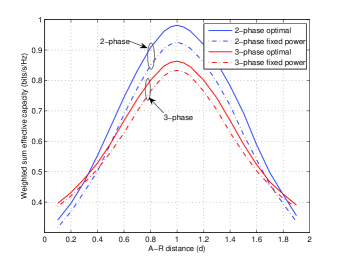
Figure 8: Impact of relay location on weighted sum effective capacity with same delay constraint $\theta_{A}=\theta_{B}=1$.

VI-B Impact of Relay Location on System Performance

In this subsection, we will consider the impact of the relay location in the two-way relay system. Here, we assume the long-term power constraints of the source nodes are $9{\rm dB}$.

First, we consider the case when source nodes have the same delay-QoS constraint that $\theta_{A}=\theta_{B}=1$. As illustrated in Fig. 8, the maximal weighted sum effective capacity is obtained when the relay is in the middle of the two source nodes no matter what transmission strategy is adopted. Meanwhile, we can observe that our proposed resource allocation policies can obviously achieve effective capacity gains in both transmission schemes. However, the benefits decrease when the relay is close to either of the source nodes. The reason is that, as a result of the severe path loss, the channel between the relay and the distant source becomes the major limit of the transmission in this case. Moreover, we can find that, on this condition, when the distance from the relay to the source node is less than 0.3, the three-phase protocol outperforms the two-phase protocol. Otherwise, the two-phase protocol has advantage over the three-phase protocol.

Next, we study the situation where the two source nodes have different delay requirements. Here, we set that $\theta_{A}=100$ and $\theta_{B}=1$. It is interesting to find from Fig. 9 that, the maximal weighted sum effective capacity for the three-phase protocol is gained when the relay is in the middle of the two sources, while the relay should be closer to the source with more stringent delay requirement if the two-phase protocol is used. Different from Fig. 8, when the distance between the relay and the node with greater $\theta$ is larger than about 1.3, the three-phase protocol can get better performance.

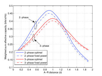
Figure 9: Impact of relay location on weighted sum effective capacity with delay constraints $\theta_{A}=100,\theta_{B}=1$.

VII Conclusion

This paper has studied the cross-layer optimization of two-way relaying under statistical delay-QoS constraints. We have focused on two main transmission protocols: three-phase transmission and two-phase transmission. By integrating the theory of effective capacity, the optimization problem for weighted sum throughput maximization in physical layer and delay provisioning in datalink layer was modeled as a long-term weighted sum effective capacity maximization problem. Then, optimal transmission policy was proposed for each protocol.

A few important conclusions have been made through extensive numerical results. Firstly, our proposed two-way relaying policies can efficiently provide delay-QoS guarantees, while there exists a tradeoff between the throughput gain and the delay-QoS provisioning. Secondly, the proposed policies significantly improve the system performance compared with the schemes without power adaptation. Especially, for the two-phase protocol, the proposed CSI-based method for successive decoding in the MAC phase has 5-10$\%$ performance improvements compared with the weight-based successive decoding. Thirdly, when the relay is located in the middle of the transmission, in terms of weighted sum effective capacity, the three-phase procotol outperforms the two-phase protocol in high SNR regime and is inferior to the two-phase protocol in low SNR regime. Last but not least, it is better to place the relay closer to the source with more stringent delay constraint for the two-phase protocol.

This work has concentrated on DF relaying with full channel information in two-way relay systems. It can be further extended to the heterogeneous networks consisting of delay-constrained and non-delay-constrained traffics. Alternative relaying protocols and transmission strategies with time adaptation or partial channel state information are also possible for future research.

Appendix A Derivation of Optimal Power Adaptation for Three-phase Two-way Relaying

Substituting the optimal rate assignment at each decoding region into the Lagrangian (20), we have

$$-\frac{\omega_{A}}{\theta_{A}}\ln\bigg{(}\int_{\boldsymbol{\gamma}\in\mathbb{R}_{1},\mathbb{R}_{3}}\big{[}1+\gamma_{3}P_{A}(\boldsymbol{\epsilon})\big{]}^{-\frac{\beta_{A}}{3}}\mathit{p}_{\boldsymbol{\gamma}}(\gamma_{1},\gamma_{2},\gamma_{3})$$

$$\times d\gamma_{1}d\gamma_{2}d\gamma_{3}+\int_{\boldsymbol{\gamma}\in\mathbb{R}_{2},\mathbb{R}_{4}}\max\big{\{}\big{[}1+\gamma_{1}P_{A}(\boldsymbol{\epsilon})\big{]}^{-\frac{\beta_{A}}{3}},$$

$$\big{[}1+\gamma_{3}P_{A}(\boldsymbol{\epsilon})+\gamma_{2}P_{R}(\boldsymbol{\epsilon})+\gamma_{3}P_{A}(\boldsymbol{\epsilon})\gamma_{2}P_{R}(\boldsymbol{\epsilon})\big{]}^{-\frac{\beta_{A}}{3}}\big{\}}$$

$$\times\mathit{p}_{\boldsymbol{\gamma}}(\gamma_{1},\gamma_{2},\gamma_{3})d\gamma_{1}d\gamma_{2}d\gamma_{3}\bigg{)}$$

$$-\frac{\omega_{B}}{\theta_{B}}\ln\bigg{(}\int_{\boldsymbol{\gamma}\in\mathbb{R}_{1},\mathbb{R}_{2}}\big{[}1+\gamma_{3}P_{B}(\boldsymbol{\epsilon})\big{]}^{-\frac{\beta_{B}}{3}}\mathit{p}_{\boldsymbol{\gamma}}(\gamma_{1},\gamma_{2},\gamma_{3})$$

$$\times d\gamma_{1}d\gamma_{2}d\gamma_{3}+\int_{\boldsymbol{\gamma}\in\mathbb{R}_{3},\mathbb{R}_{4}}\max\big{\{}\big{[}1+\gamma_{2}P_{B}(\boldsymbol{\epsilon})\big{]}^{-\frac{\beta_{B}}{3}},$$

$$\big{[}1+\gamma_{3}P_{B}(\boldsymbol{\epsilon})+\gamma_{1}P_{R}(\boldsymbol{\epsilon})+\gamma_{3}P_{B}(\boldsymbol{\epsilon})\gamma_{1}P_{R}(\boldsymbol{\epsilon})\big{]}^{-\frac{\beta_{B}}{3}}\big{\}}$$

$$\times\mathit{p}_{\boldsymbol{\gamma}}(\gamma_{1},\gamma_{2},\gamma_{3})d\gamma_{1}d\gamma_{2}d\gamma_{3}\bigg{)}+\lambda_{A}\big{(}\overline{P_{A}}-\mathbb{E}_{\boldsymbol{\gamma}}[P_{A}(\boldsymbol{\epsilon})]\big{)}$$

$$+\lambda_{B}\big{(}\overline{P_{B}}-\mathbb{E}_{\boldsymbol{\gamma}}[P_{B}(\boldsymbol{\epsilon})]\big{)}+\lambda_{R}\big{(}\overline{P_{R}}-\mathbb{E}_{\boldsymbol{\gamma}}[P_{R}(\boldsymbol{\epsilon})]\big{)},$$ (60)

where $p_{\boldsymbol{\gamma}}$ is the distribution function of $\boldsymbol{\gamma}$.

A-1 Region $\mathbb{R}_{1}(\gamma_{1}\leq\gamma_{3},\gamma_{2}\leq\gamma_{3})$

Setting the partial derivative at $P_{A}(\boldsymbol{\epsilon})$ equal to zero, we can obtain

$$\int_{\boldsymbol{\gamma}\in\mathbb{R}_{1}} \bigg{\{}\frac{\omega_{A}}{\theta_{A}\phi_{1}}\cdot\frac{\beta_{A}\gamma_{3}}{3}\big{[}1+\gamma_{3}P_{A}(\boldsymbol{\epsilon})\big{]}^{-\frac{\beta_{A}+3}{3}}-\lambda_{A}\bigg{\}}$$ (61)

$$\times\mathit{p}_{\boldsymbol{\gamma}}(\gamma_{1},\gamma_{2},\gamma_{3})d\gamma_{1}d\gamma_{2}d\gamma_{3}=0,$$

which gives

$$\frac{\omega_{A}\gamma_{3}}{\sigma\phi_{1}}\big{[}1+\gamma_{3}P_{A}(\boldsymbol{\epsilon})\big{]}^{-\frac{\beta_{A}+3}{3}}=\lambda_{A}.$$ (62)

Hence, the optimal $P_{A}(\boldsymbol{\epsilon})$ can be obtained as in (24). The optimal $P_{B}(\boldsymbol{\epsilon})$ can be achieved using the same method.

A-2 Region $\mathbb{R}_{2}(\gamma_{1}>\gamma_{3},\gamma_{2}\leq\gamma_{3})$

It is easy to see that the maximum $R_{A}(\boldsymbol{\epsilon})$ is achieved when

$$C\big{(}\gamma_{1}P_{A}(\boldsymbol{\epsilon})\big{)}=C\big{(}\gamma_{3}P_{A}(\boldsymbol{\epsilon})\big{)}+C\big{(}\gamma_{2}P_{R}(\boldsymbol{\epsilon})\big{)},$$ (63)

which in turn gives

$$P_{R}(\boldsymbol{\epsilon})=\frac{(\gamma_{1}-\gamma_{3})P_{A}(\boldsymbol{\epsilon})}{\gamma_{2}\big{[}1+\gamma_{3}P_{A}(\boldsymbol{\epsilon})\big{]}}.$$ (64)

We substitute (64) into (A), take the partial derivative at $P_{A}(\boldsymbol{\epsilon})$, and then obtain

$$\int_{\boldsymbol{\gamma}\in\mathbb{R}_{2}} \bigg{\{}\frac{\omega_{A}}{\theta_{A}\phi_{1}}\cdot\frac{\beta_{A}\gamma_{1}}{3}\big{[}1+\gamma_{1}P_{A}(\boldsymbol{\epsilon})\big{]}^{-\frac{\beta_{A}+3}{3}}$$ (65)

$$-\frac{\lambda_{R}(\gamma_{1}-\gamma_{3})}{\gamma_{2}}\cdot\frac{1}{\big{[}1+\gamma_{3}P_{A}(\boldsymbol{\epsilon})\big{]}^{2}}-\lambda_{A}\bigg{\}}$$

$$\times\mathit{p}_{\boldsymbol{\gamma}}(\gamma_{1},\gamma_{2},\gamma_{3})d\gamma_{1}d\gamma_{2}d\gamma_{3}=0,$$

which yields (30). Therefore, the optimal $P_{A}(\boldsymbol{\epsilon})$ is given in (29). The power allocation for $P_{B}(\boldsymbol{\epsilon})$ is same as $\mathbb{R}_{1}$.

A-3 Region $\mathbb{R}_{3}(\gamma_{1}\leq\gamma_{3},\gamma_{2}>\gamma_{3})$

We can use the similar method as $\mathbb{R}_{2}$ to get the optimal power allocation for $P_{A}(\boldsymbol{\epsilon}),P_{B}(\boldsymbol{\epsilon})$.

A-4 Region $\mathbb{R}_{4}(\gamma_{1}>\gamma_{3},\gamma_{2}>\gamma_{3})$

According to (7) and (9), the maximum rates are achieved when

$$C\big{(}\gamma_{1}P_{A}(\boldsymbol{\epsilon})\big{)} = C\big{(}\gamma_{3}P_{A}(\boldsymbol{\epsilon})\big{)}+C\big{(}\gamma_{2}P_{R}(\boldsymbol{\epsilon})\big{)},$$ (66)

$$C\big{(}\gamma_{2}P_{B}(\boldsymbol{\epsilon})\big{)} = C\big{(}\gamma_{3}P_{B}(\boldsymbol{\epsilon})\big{)}+C\big{(}\gamma_{1}P_{R}(\boldsymbol{\epsilon})\big{)},$$ (67)

which offers

$$P_{R}(\boldsymbol{\epsilon})=\frac{(\gamma_{1}-\gamma_{3})P_{A}(\boldsymbol{\epsilon})}{\gamma_{2}\big{[}1+\gamma_{3}P_{A}(\boldsymbol{\epsilon})\big{]}}=\frac{(\gamma_{2}-\gamma_{3})P_{B}(\boldsymbol{\epsilon})}{\gamma_{1}\big{[}1+\gamma_{3}P_{B}(\boldsymbol{\epsilon})\big{]}}.$$ (68)

Therefore,

$$P_{A}(\boldsymbol{\epsilon})=\frac{P_{B}(\boldsymbol{\epsilon})}{\tau+(\tau-1)\gamma_{3}P_{B}(\boldsymbol{\epsilon})},$$ (69)

$$P_{B}(\boldsymbol{\epsilon})=\frac{\tau P_{A}(\boldsymbol{\epsilon})}{1+(1-\tau)\gamma_{3}P_{A}(\boldsymbol{\epsilon})},$$ (70)

where $\tau$ is given in (33). If $0<\tau\leq 1$, it always holds that if $P_{A}(\boldsymbol{\epsilon})>0$, then $P_{B}(\boldsymbol{\epsilon})>0$. Otherwise, if $\tau>1$, then if $P_{B}(\boldsymbol{\epsilon})>0$, it is sure that $P_{A}(\boldsymbol{\epsilon})>0$. In the following, we assume $0<\tau\leq 1$, while the power allocation policies for $\tau>1$ can be obtained in the same manner.

Substituting (68) and (70) into (A) and taking the the partial derivative of $P_{A}(\boldsymbol{\epsilon})$, we can get

$$\int_{\boldsymbol{\gamma}\in\mathbb{R}_{4}} \bigg{\{}\frac{\omega_{A}}{\theta_{A}\phi_{1}}\cdot\frac{\beta_{A}\gamma_{1}}{3}\big{[}1+\gamma_{1}P_{A}(\boldsymbol{\epsilon})\big{]}^{-\frac{\beta_{A}+3}{3}}$$

$$+\frac{\omega_{B}}{\theta_{B}\phi_{2}}\cdot\frac{\beta_{B}}{3}\cdot\frac{\tau\gamma_{2}}{\big{[}1+(1-\tau)\gamma_{3}P_{A}(\boldsymbol{\epsilon})\big{]}^{2}}$$

$$\times\bigg{[}1+\frac{\tau\gamma_{2}P_{A}(\boldsymbol{\epsilon})}{1+(1-\tau)\gamma_{3}P_{A}(\boldsymbol{\epsilon})}\bigg{]}^{-\frac{\beta_{B}+3}{3}}-\lambda_{A}$$

$$-\frac{\tau\lambda_{B}}{\big{[}1+(1-\tau)\gamma_{3}P_{A}(\boldsymbol{\epsilon})\big{]}^{2}}-\frac{\lambda_{R}(\gamma_{1}-\gamma_{3})}{\gamma_{2}}$$

$$\times\frac{1}{\big{[}1+\gamma_{3}P_{A}(\boldsymbol{\epsilon})\big{]}^{2}}\bigg{\}}\mathit{p}_{\boldsymbol{\gamma}}(\gamma_{1},\gamma_{2},\gamma_{3})d\gamma_{1}d\gamma_{2}d\gamma_{3}=0,$$

which can be simplified as equation (IV-A4). Thus, the optimal $P_{A}$ is the solution of (IV-A4) as stated in (34). The optimal $P_{B}$ can be obtained similarly.

Appendix B Derivation of Optimal $P_{A}(\boldsymbol{\epsilon})$ and $P_{B}(\boldsymbol{\epsilon})$ for Two-phase Two-way Relaying

According to the achievable rates in the decoding region $(\mathbb{R}^{\prime}_{1},\mathbb{R}^{\prime}_{2})$, we can rewrite (43) without loss of optimality as

$$-\frac{\omega_{A}}{\theta_{A}}\ln\bigg{(}\int_{\boldsymbol{\gamma}\in\mathbb{R}^{\prime}_{1}}\bigg{[}1+\frac{\gamma_{1}P_{A}(\boldsymbol{\epsilon})}{1+\gamma_{2}P_{B}(\boldsymbol{\epsilon})}\bigg{]}^{-\frac{\beta_{A}}{2}}\mathit{p}_{\boldsymbol{\gamma}}(\gamma_{1},\gamma_{2})d\gamma_{1}d\gamma_{2}$$

$$+\int_{\boldsymbol{\gamma}\in\mathbb{R}^{\prime}_{2}}\big{[}1+\gamma_{1}P_{A}(\boldsymbol{\epsilon})\big{]}^{-\frac{\beta_{A}}{2}}\mathit{p}_{\boldsymbol{\gamma}}(\gamma_{1},\gamma_{2})d\gamma_{1}d\gamma_{2}\bigg{)}$$

$$-\frac{\omega_{B}}{\theta_{B}}\ln\bigg{(}\int_{\boldsymbol{\gamma}\in\mathbb{R}^{\prime}_{1}}\big{[}1+\gamma_{2}P_{B}(\boldsymbol{\epsilon})\big{]}^{-\frac{\beta_{B}}{2}}\mathit{p}_{\boldsymbol{\gamma}}(\gamma_{1},\gamma_{2})d\gamma_{1}d\gamma_{2}$$

$$+\int_{\boldsymbol{\gamma}\in\mathbb{R}^{\prime}_{2}}\bigg{[}1+\frac{\gamma_{2}P_{B}(\boldsymbol{\epsilon})}{1+\gamma_{1}P_{A}(\boldsymbol{\epsilon})}\bigg{]}^{-\frac{\beta_{B}}{2}}\mathit{p}_{\boldsymbol{\gamma}}(\gamma_{1},\gamma_{2})d\gamma_{1}d\gamma_{2}\bigg{)}$$

$$+\bigg{(}\int_{\boldsymbol{\gamma}\in\mathbb{R}^{\prime}_{1}}\frac{\mu_{A}}{\theta_{A}}\bigg{[}1+\frac{\gamma_{1}P_{A}(\boldsymbol{\epsilon})}{1+\gamma_{2}P_{B}(\boldsymbol{\epsilon})}\bigg{]}^{-\frac{\beta_{A}}{2}}\mathit{p}_{\boldsymbol{\gamma}}(\gamma_{1},\gamma_{2})d\gamma_{1}d\gamma_{2}$$

$$+\int_{\boldsymbol{\gamma}\in\mathbb{R}^{\prime}_{2}}\frac{\mu_{A}}{\theta_{A}}\big{[}1+\gamma_{1}P_{A}(\boldsymbol{\epsilon})\big{]}^{-\frac{\beta_{A}}{2}}\mathit{p}_{\boldsymbol{\gamma}}(\gamma_{1},\gamma_{2})d\gamma_{1}d\gamma_{2}\bigg{)}$$

$$+\bigg{(}\int_{\boldsymbol{\gamma}\in\mathbb{R}^{\prime}_{1}}\frac{\mu_{B}}{\theta_{B}}\big{[}1+\gamma_{2}P_{B}(\boldsymbol{\epsilon})\big{]}^{-\frac{\beta_{B}}{2}}\mathit{p}_{\boldsymbol{\gamma}}(\gamma_{1},\gamma_{2})d\gamma_{1}d\gamma_{2}$$

$$+\int_{\boldsymbol{\gamma}\in\mathbb{R}^{\prime}_{2}}\frac{\mu_{B}}{\theta_{B}}\bigg{[}1+\frac{\gamma_{2}P_{B}(\boldsymbol{\epsilon})}{1+\gamma_{1}P_{A}(\boldsymbol{\epsilon})}\bigg{]}^{-\frac{\beta_{B}}{2}}\mathit{p}_{\boldsymbol{\gamma}}(\gamma_{1},\gamma_{2})d\gamma_{1}d\gamma_{2}\bigg{)}$$

$$+\lambda_{A}\big{(}\overline{P_{A}}-\mathbb{E}_{\boldsymbol{\gamma}}[P_{A}(\boldsymbol{\epsilon})]\big{)}+\lambda_{B}\big{(}\overline{P_{B}}-\mathbb{E}_{\boldsymbol{\gamma}}[P_{B}(\boldsymbol{\epsilon})]\big{)},$$ (72)

The partial derivative of (B) with respect to $P_{A}(\boldsymbol{\epsilon})$ is given by

$$-\frac{\omega_{A}}{\theta_{A}\phi^{\prime}_{1}}\bigg{(}\int_{\boldsymbol{\gamma}\in\mathbb{R}^{\prime}_{1}}-\frac{\beta_{A}\gamma_{1}}{2\big{[}1+\gamma_{2}P_{B}(\boldsymbol{\epsilon})\big{]}}$$ (73)

$$\times\bigg{[}1+\frac{\gamma_{1}P_{A}(\boldsymbol{\epsilon})}{1+\gamma_{2}P_{B}(\boldsymbol{\epsilon})}\bigg{]}^{-\frac{\beta_{A}}{2}-1}\mathit{p}_{\boldsymbol{\gamma}}(\gamma_{1},\gamma_{2})d\gamma_{1}d\gamma_{2}$$

$$+\int_{\boldsymbol{\gamma}\in\mathbb{R}^{\prime}_{2}}-\frac{\beta_{A}\gamma_{1}}{2}\big{[}1+\gamma_{1}P_{A}(\boldsymbol{\epsilon})\big{]}^{-\frac{\beta_{A}}{2}-1}\mathit{p}_{\boldsymbol{\gamma}}(\gamma_{1},\gamma_{2})d\gamma_{1}d\gamma_{2}\bigg{)}$$

$$-\frac{\omega_{B}}{\theta_{B}\phi^{\prime}_{2}}\bigg{(}\int_{\boldsymbol{\gamma}\in\mathbb{R}^{\prime}_{2}}\frac{\beta_{B}\gamma_{1}\gamma_{2}P_{B}(\boldsymbol{\epsilon})}{2\big{[}1+\gamma_{1}P_{A}(\boldsymbol{\epsilon})\big{]}^{2}}$$

$$\times\bigg{[}1+\frac{\gamma_{2}P_{B}(\boldsymbol{\epsilon})}{1+\gamma_{1}P_{A}(\boldsymbol{\epsilon})}\bigg{]}^{-\frac{\beta_{B}}{2}-1}\mathit{p}_{\boldsymbol{\gamma}}(\gamma_{1},\gamma_{2})d\gamma_{1}d\gamma_{2}\bigg{)}$$

$$+\bigg{(}\int_{\boldsymbol{\gamma}\in\mathbb{R}^{\prime}_{1}}-\frac{\mu_{A}\beta_{A}\gamma_{1}}{2\theta_{A}\big{[}1+\gamma_{2}P_{B}(\boldsymbol{\epsilon})\big{]}}$$

$$\times\bigg{[}1+\frac{\gamma_{1}P_{A}(\boldsymbol{\epsilon})}{1+\gamma_{2}P_{B}(\boldsymbol{\epsilon})}\bigg{]}^{-\frac{\beta_{A}}{2}-1}\mathit{p}_{\boldsymbol{\gamma}}(\gamma_{1},\gamma_{2})d\gamma_{1}d\gamma_{2}$$

$$+\int_{\boldsymbol{\gamma}\in\mathbb{R}^{\prime}_{2}}-\frac{\mu_{A}\beta_{A}\gamma_{1}}{2\theta_{A}}\big{[}1+\gamma_{1}P_{A}(\boldsymbol{\epsilon})\big{]}^{-\frac{\beta_{A}}{2}-1}\mathit{p}_{\boldsymbol{\gamma}}(\gamma_{1},\gamma_{2})d\gamma_{1}d\gamma_{2}\bigg{)}$$

$$+\bigg{(}\int_{\boldsymbol{\gamma}\in\mathbb{R}^{\prime}_{2}}\frac{\mu_{B}\beta_{B}\gamma_{1}\gamma_{2}P_{B}(\boldsymbol{\epsilon})}{2\theta_{B}\big{[}1+\gamma_{1}P_{A}(\boldsymbol{\epsilon})\big{]}^{2}}\bigg{[}1+\frac{\gamma_{2}P_{B}(\boldsymbol{\epsilon})}{1+\gamma_{1}P_{A}(\boldsymbol{\epsilon})}\bigg{]}^{-\frac{\beta_{B}}{2}-1}$$

$$\times\mathit{p}_{\boldsymbol{\gamma}}(\gamma_{1},\gamma_{2})d\gamma_{1}d\gamma_{2}\bigg{)}-\lambda_{A}.$$

By differentiating on $P_{B}(\boldsymbol{\epsilon})$ of (B), the similar result can be obtained as

$$-\frac{\omega_{A}}{\theta_{A}\phi^{\prime}_{1}}\bigg{(}\int_{\boldsymbol{\gamma}\in\mathbb{R}^{\prime}_{1}}\frac{\beta_{A}\gamma_{1}\gamma_{2}P_{A}(\boldsymbol{\epsilon})}{2\big{[}1+\gamma_{2}P_{B}(\boldsymbol{\epsilon})\big{]}^{2}}$$

$$\times\bigg{[}1+\frac{\gamma_{1}P_{A}(\boldsymbol{\epsilon})}{1+\gamma_{2}P_{B}(\boldsymbol{\epsilon})}\bigg{]}^{-\frac{\beta_{A}}{2}-1}\mathit{p}_{\boldsymbol{\gamma}}(\gamma_{1},\gamma_{2})d\gamma_{1}d\gamma_{2}\bigg{)}$$

$$-\frac{\omega_{B}}{\theta_{B}\phi^{\prime}_{2}}\bigg{(}\int_{\boldsymbol{\gamma}\in\mathbb{R}^{\prime}_{1}}-\frac{\beta_{B}\gamma_{2}}{2}\big{[}1+\gamma_{2}P_{B}(\boldsymbol{\epsilon})\big{]}^{-\frac{\beta_{B}}{2}-1}$$

$$\times\mathit{p}_{\boldsymbol{\gamma}}(\gamma_{1},\gamma_{2})d\gamma_{1}d\gamma_{2}+\int_{\boldsymbol{\gamma}\in\mathbb{R}^{\prime}_{2}}-\frac{\beta_{B}\gamma_{2}}{2\big{[}1+\gamma_{1}P_{A}(\boldsymbol{\epsilon})\big{]}}$$

$$\times\bigg{[}1+\frac{\gamma_{2}P_{B}(\boldsymbol{\epsilon})}{1+\gamma_{1}P_{A}(\boldsymbol{\epsilon})}\bigg{]}^{-\frac{\beta_{B}}{2}-1}\mathit{p}_{\boldsymbol{\gamma}}(\gamma_{1},\gamma_{2})d\gamma_{1}d\gamma_{2}\bigg{)}$$

$$+\bigg{(}\int_{\boldsymbol{\gamma}\in\mathbb{R}^{\prime}_{1}}\frac{\mu_{A}\beta_{A}\gamma_{1}\gamma_{2}P_{A}(\boldsymbol{\epsilon})}{2\theta_{A}\big{[}1+\gamma_{2}P_{B}(\boldsymbol{\epsilon})\big{]}^{2}}\bigg{[}1+\frac{\gamma_{1}P_{A}(\boldsymbol{\epsilon})}{1+\gamma_{2}P_{B}(\boldsymbol{\epsilon})}\bigg{]}^{-\frac{\beta_{A}}{2}-1}$$

$$\times\mathit{p}_{\boldsymbol{\gamma}}(\gamma_{1},\gamma_{2})d\gamma_{1}d\gamma_{2}\bigg{)}+\bigg{(}\int_{\boldsymbol{\gamma}\in\mathbb{R}^{\prime}_{1}}-\frac{\mu_{B}\beta_{B}\gamma_{2}}{2\theta_{B}}$$

$$\times\big{[}1+\gamma_{2}P_{B}(\boldsymbol{\epsilon})\big{]}^{-\frac{\beta_{B}}{2}-1}\mathit{p}_{\boldsymbol{\gamma}}(\gamma_{1},\gamma_{2})d\gamma_{1}d\gamma_{2}$$

$$+\int_{\boldsymbol{\gamma}\in\mathbb{R}^{\prime}_{2}}-\frac{\mu_{B}\beta_{B}\gamma_{2}}{2\theta_{B}\big{[}1+\gamma_{1}P_{A}(\boldsymbol{\epsilon})\big{]}}\bigg{[}1+\frac{\gamma_{2}P_{B}(\boldsymbol{\epsilon})}{1+\gamma_{1}P_{A}(\boldsymbol{\epsilon})}\bigg{]}^{-\frac{\beta_{B}}{2}-1}$$

$$\times\mathit{p}_{\boldsymbol{\gamma}}(\gamma_{1},\gamma_{2})d\gamma_{1}d\gamma_{2}\bigg{)}-\lambda_{B}.$$ (74)

Let the derivatives equal to zero. If $\boldsymbol{\gamma}\in\mathbb{R}^{\prime}_{1}$, from (73), the optimal condition should satisfy

$$\int_{\boldsymbol{\gamma}\in\mathbb{R}^{\prime}_{1}}\bigg{\{}\bigg{(}\frac{\omega_{A}\beta_{A}}{2\theta_{A}\phi^{\prime}_{1}}-\frac{\mu_{A}\beta_{A}}{2\theta_{A}}\bigg{)}\frac{\gamma_{1}}{1+\gamma_{2}P_{B}(\boldsymbol{\epsilon})}$$

$$\times\bigg{[}1+\frac{\gamma_{1}P_{A}(\boldsymbol{\epsilon})}{1+\gamma_{2}P_{B}(\boldsymbol{\epsilon})}\bigg{]}^{-\frac{\beta_{A}+2}{2}}-\lambda_{A}\bigg{\}}\mathit{p}_{\boldsymbol{\gamma}}(\gamma_{1},\gamma_{2})d\gamma_{1}d\gamma_{2}=0,$$

which gives

$$\frac{\gamma_{1}(\omega_{A}{\phi^{\prime}_{1}}^{-1}-\mu_{A})}{1+\gamma_{2}P_{B}(\boldsymbol{\epsilon})}\bigg{[}1+\frac{\gamma_{1}P_{A}(\boldsymbol{\epsilon})}{1+\gamma_{2}P_{B}(\boldsymbol{\epsilon})}\bigg{]}^{-\frac{\beta_{A}+2}{2}}=\delta\lambda_{A}.$$ (76)

From (B), we can find the following optimality condition

$$\int_{\boldsymbol{\gamma}\in\mathbb{R}^{\prime}_{1}}\bigg{\{}\bigg{(}\frac{\omega_{B}\beta_{B}}{2\theta_{B}\phi^{\prime}_{2}}-\frac{\mu_{B}\beta_{B}}{2\theta_{B}}\bigg{)}\gamma_{2}\big{[}1+\gamma_{2}P_{B}(\boldsymbol{\epsilon})\big{]}^{-\frac{\beta_{B}+2}{2}}$$

$$-\lambda_{B}-\bigg{(}\frac{\omega_{A}\beta_{A}}{2\theta_{A}\phi^{\prime}_{1}}-\frac{\mu_{A}\beta_{A}}{2\theta_{A}}\bigg{)}\frac{\gamma_{1}\gamma_{2}P_{A}(\boldsymbol{\epsilon})}{\big{[}1+\gamma_{2}P_{B}(\boldsymbol{\epsilon})\big{]}^{2}}$$

$$\times\bigg{[}1+\frac{\gamma_{1}P_{A}(\boldsymbol{\epsilon})}{1+\gamma_{2}P_{B}(\boldsymbol{\epsilon})}\bigg{]}^{-\frac{\beta_{A}+2}{2}}\bigg{\}}\mathit{p}_{\boldsymbol{\gamma}}(\gamma_{1},\gamma_{2})d\gamma_{1}d\gamma_{2}=0,$$ (77)

which offers

$$\gamma_{2}(\omega_{B}{\phi^{\prime}_{2}}^{-1}-\mu_{B})\big{[}1+\gamma_{2}P_{B}(\boldsymbol{\epsilon})\big{]}^{-\frac{\beta_{B}+2}{2}}-\delta\lambda_{B}$$

$$-\frac{(\omega_{A}{\phi^{\prime}_{1}}^{-1}-\mu_{A})\gamma_{1}\gamma_{2}P_{A}(\boldsymbol{\epsilon})}{\big{[}1+\gamma_{2}P_{B}(\boldsymbol{\epsilon})\big{]}^{2}}\bigg{[}1+\frac{\gamma_{1}P_{A}(\boldsymbol{\epsilon})}{1+\gamma_{2}P_{B}(\boldsymbol{\epsilon})}\bigg{]}^{-\frac{\beta_{A}+2}{2}}=0.$$

Replacing (76) into (B), and after some calculations, we can obtain the optimal power allocation of $P_{A}(\boldsymbol{\epsilon})$ and $P_{B}(\boldsymbol{\epsilon})$ in (52) and (V-A1).

Appendix C Derivation of Optimal Partition Criterion for Two-phase Two-way Relaying

Here we only focus on the derivation for the threshold $\gamma_{2}^{th}$, while $\gamma_{1}^{th}$ can be obtained by the same way. Let we write the optimal $\gamma_{2}^{th}$ as a function of $\gamma_{1}$, i.e., $\gamma_{2}^{th}=f^{*}(\gamma_{1})$, where $f^{*}(\gamma_{1})$ is the optimal function. We define $f(\gamma_{1})=f^{*}(\gamma_{1})+sg(\gamma_{1})$, where $s$ is any constant and $g(\gamma_{1})$ represents arbitrary variation. Thus, (43) can be rewritten as

$$~{}\mathcal{J}(f(\gamma_{1}))$$

$$=-\frac{\omega_{A}}{\theta_{A}}\ln\bigg{(}\int_{0}^{\infty}\int_{0}^{f(\gamma_{1})}\bigg{[}1+\frac{\gamma_{1}P_{A}(\boldsymbol{\epsilon})}{1+\gamma_{2}P_{B}(\boldsymbol{\epsilon})}\bigg{]}^{-\frac{\beta_{A}}{2}}\mathit{p}_{\boldsymbol{\gamma}}(\gamma_{1},\gamma_{2})$$

$$\times d\gamma_{1}d\gamma_{2}+\int_{0}^{\infty}\int_{f(\gamma_{1})}^{\infty}\big{[}1+\gamma_{1}P_{A}(\boldsymbol{\epsilon})\big{]}^{-\frac{\beta_{A}}{2}}\mathit{p}_{\boldsymbol{\gamma}}(\gamma_{1},\gamma_{2})d\gamma_{1}d\gamma_{2}\bigg{)}$$

$$-\frac{\omega_{B}}{\theta_{B}}\ln\bigg{(}\int_{0}^{\infty}\int_{0}^{f(\gamma_{1})}\big{[}1+\gamma_{2}P_{B}(\boldsymbol{\epsilon})\big{]}^{-\frac{\beta_{B}}{2}}\mathit{p}_{\boldsymbol{\gamma}}(\gamma_{1},\gamma_{2})d\gamma_{1}d\gamma_{2}$$

$$+\int_{0}^{\infty}\int_{f(\gamma_{1})}^{\infty}\bigg{[}1+\frac{\gamma_{2}P_{B}(\boldsymbol{\epsilon})}{1+\gamma_{1}P_{A}(\boldsymbol{\epsilon})}\bigg{]}^{-\frac{\beta_{B}}{2}}\mathit{p}_{\boldsymbol{\gamma}}(\gamma_{1},\gamma_{2})d\gamma_{1}d\gamma_{2}\bigg{)}$$

$$+\bigg{(}\int_{0}^{\infty}\int_{0}^{f(\gamma_{1})}\frac{\mu_{A}}{\theta_{A}}\bigg{[}1+\frac{\gamma_{1}P_{A}(\boldsymbol{\epsilon})}{1+\gamma_{2}P_{B}(\boldsymbol{\epsilon})}\bigg{]}^{-\frac{\beta_{A}}{2}}\mathit{p}_{\boldsymbol{\gamma}}(\gamma_{1},\gamma_{2})d\gamma_{1}d\gamma_{2}$$

$$+\int_{0}^{\infty}\int_{f(\gamma_{1})}^{\infty}\frac{\mu_{A}}{\theta_{A}}\big{[}1+\gamma_{1}P_{A}(\boldsymbol{\epsilon})\big{]}^{-\frac{\beta_{A}}{2}}\mathit{p}_{\boldsymbol{\gamma}}(\gamma_{1},\gamma_{2})d\gamma_{1}d\gamma_{2}\bigg{)}$$

$$+\bigg{(}\int_{0}^{\infty}\int_{0}^{f(\gamma_{1})}\frac{\mu_{B}}{\theta_{B}}\big{[}1+\gamma_{2}P_{B}(\boldsymbol{\epsilon})\big{]}^{-\frac{\beta_{B}}{2}}\mathit{p}_{\boldsymbol{\gamma}}(\gamma_{1},\gamma_{2})d\gamma_{1}d\gamma_{2}$$

$$+\int_{0}^{\infty}\int_{f(\gamma_{1})}^{\infty}\frac{\mu_{B}}{\theta_{B}}\bigg{[}1+\frac{\gamma_{2}P_{B}(\boldsymbol{\epsilon})}{1+\gamma_{1}P_{A}(\boldsymbol{\epsilon})}\bigg{]}^{-\frac{\beta_{B}}{2}}\mathit{p}_{\boldsymbol{\gamma}}(\gamma_{1},\gamma_{2})d\gamma_{1}d\gamma_{2}\bigg{)}$$

$$+\lambda_{A}\big{(}\overline{P_{A}}-\mathbb{E}_{\boldsymbol{\gamma}}[P_{A}(\boldsymbol{\epsilon})]\big{)}+\lambda_{B}\big{(}\overline{P_{B}}-\mathbb{E}_{\boldsymbol{\gamma}}[P_{B}(\boldsymbol{\epsilon})]\big{)}.$$ (79)

Intuitively, $\mathcal{J}\big{(}f(\gamma_{1})\big{)}$ gains its optimal value when $s=0$, namely, the derivative of $\mathcal{J}\big{(}f(\gamma_{1})\big{)}$ is equal to zero when $s=0$. Therefore, to obtain the optimal condition, it is necessary to satisfy [30]

$$\frac{\emph{d}}{\emph{d}s}\big{(}\mathcal{J}\big{(}f(\gamma_{1})\big{)}\big{)}\bigg{|}_{s=0}=0.$$ (80)

Then, it follows that

$$\int_{0}^{\infty}\bigg{\{}-\bigg{(}\frac{\omega_{A}}{\theta_{A}\phi^{\prime}_{1}}-\frac{\mu_{A}}{\theta_{A}}\bigg{)}\bigg{(}\bigg{[}1+\frac{\gamma_{1}P_{A}(\boldsymbol{\epsilon})}{1+f^{*}(\gamma_{1})P_{B}(\boldsymbol{\epsilon})}\bigg{]}^{-\frac{\beta_{A}}{2}}$$

$$-\big{[}1+\gamma_{1}P_{A}(\boldsymbol{\epsilon})\big{]}^{-\frac{\beta_{A}}{2}}\bigg{)}-\bigg{(}\frac{\omega_{B}}{\theta_{B}\phi^{\prime}_{2}}-\frac{\mu_{B}}{\theta_{B}}\bigg{)}$$

$$\times\bigg{(}\big{[}1+f^{*}(\gamma_{1})P_{B}(\boldsymbol{\epsilon})\big{]}^{-\frac{\beta_{B}}{2}}-\bigg{[}1+\frac{f^{*}(\gamma_{1})P_{B}(\boldsymbol{\epsilon})}{1+\gamma_{1}P_{A}(\boldsymbol{\epsilon})}\bigg{]}^{-\frac{\beta_{B}}{2}}\bigg{)}\bigg{\}}$$

$$\times\mathit{p}_{\boldsymbol{\gamma}}(\gamma_{1},f^{*}(\gamma_{1}))g(\gamma_{1})d\gamma_{1}=0.$$ (81)

Since the above equation needs to be hold for any $g(\gamma_{1})$, we can obtain

$$\frac{\big{[}1+\frac{\gamma_{1}P_{A}(\boldsymbol{\epsilon})}{1+f^{*}(\gamma_{1})P_{B}(\boldsymbol{\epsilon})}\big{]}^{-\frac{\beta_{A}}{2}}-\big{[}1+\gamma_{1}P_{A}(\boldsymbol{\epsilon})\big{]}^{-\frac{\beta_{A}}{2}}}{\big{[}1+\frac{f^{*}(\gamma_{1})P_{B}(\boldsymbol{\epsilon})}{1+\gamma_{1}P_{A}(\boldsymbol{\epsilon})}\big{]}^{-\frac{\beta_{B}}{2}}-\big{[}1+f^{*}(\gamma_{1})P_{B}(\boldsymbol{\epsilon})\big{]}^{-\frac{\beta_{B}}{2}}}$$ (82)

$$= \frac{\theta_{A}(\omega_{B}{\phi^{\prime}_{2}}^{-1}-\mu_{B})}{\theta_{B}(\omega_{A}{\phi^{\prime}_{1}}^{-1}-\mu_{A})}\triangleq K.$$

Obviously, $K\geq 0$ for all cases. Specifically, $\gamma_{2}^{th}=f^{*}(\gamma_{1})$ should be positive, otherwise it would not be well-defined in (82).

Cen Lin received the B.S. degree in electrical engineering from Shanghai Jiao Tong University, Shanghai, China, in 2010. He is currently pursuing a dual M.S degree in electrical and computer engineering from Shanghai Jiao Tong University and Georgia Institute of Technology. His research interests include cooperative communications, physical layer network coding, and resource allocation for QoS provisioning.

Yuan Liu (S’11) received the B.S. degree from Hunan University of Science and Technology, Xiangtan, China, in 2006, and the M.S. degree from Guangdong University of Technology, Guangzhou, China, in 2009, both in Communications Engineering and with the highest honors. He is currently pursuing his Ph.D. degree at the Department of Electrical Engineering in Shanghai Jiao Tong University. His current research interests include cooperative communications, network coding, resource allocation, physical layer security, MIMO and OFDM techniques. He is the recipient of the Guangdong Province Excellent Master Theses Award in 2010. He has been honored as an Exemplary Reviewer of the IEEE Communications Letters. He is also awarded the IEEE Student Travel Grant for IEEE ICC 2012. He is a student member of the IEEE.

Meixia Tao (S’00-M’04-SM’10) received the B.S. degree in electronic engineering from Fudan University, Shanghai, China, in 1999, and the Ph.D. degree in electrical and electronic engineering from Hong Kong University of Science and Technology in 2003. She is currently an Associate Professor with the Department of Electronic Engineering, Shanghai Jiao Tong University, China. From August 2003 to August 2004, she was a Member of Professional Staff at Hong Kong Applied Science and Technology Research Institute Co. Ltd. From August 2004 to December 2007, she was with the Department of Electrical and Computer Engineering, National University of Singapore, as an Assistant Professor. Her current research interests include cooperative transmission, physical layer network coding, resource allocation of OFDM networks, and MIMO techniques. Dr. Tao is an Editor for the IEEE Wireless Communications Letters, an Associate Editor for the IEEE Communications Letters and an Editor for the Journal of Communications and Networks. She was on the Editorial Board of the IEEE Transactions on Wireless Communications from 2007 to 2011. She served as Track/Symposium Co-Chair for APCC09, ChinaCom09, IEEE ICCCN07, and IEEE ICCCAS07. She has also served as Technical Program Committee member for various conferences, including IEEE INFOCOM, IEEE GLOBECOM, IEEE ICC, IEEE WCNC, and IEEE VTC. Dr. Tao is the recipient of the IEEE ComSoC Asia-Pacific Outstanding Young Researcher Award in 2009.

References

• [1] C. Lin, Y. Liu, and M. Tao, “Cross-Layer Resource Allocation of Two-Way Relaying for Statistical Delay-QoS Guarantees”, in Proc. IEEE ICC, Ottawa, Canada, Jun. 2012.
• [2] S. Zhang, S. C. Liew, and P. P. Lam, “Physical-Layer Network Coding”, in Proc. IEEE MobiCom, pp. 358-365, Sep. 2006.
• [3] P. Popovski and H. Yomo, “Physical Network Coding in Two-Way Wireless Relay Channels”, in Proc. IEEE ICC, pp.707-712, Jun. 2007.
• [4] B. Rankov and A. Wittneben, “Spectral Efficienct Protocols for Half-Duplex Fading Relay Channels”, IEEE J. Sel. Areas Commun., vol. 25, no. 2, pp. 379-389, Feb. 2007.
• [5] S. J. Kim, P. Mitran, and V. Tarokh, “Performance Bounds for Bidirectional Coded Cooperation Protocols”, IEEE Trans. Inf. Theory, vol. 54, no. 11, pp. 5235-5241, Nov. 2008.
• [6] J. Liu, M. Tao and Y. Xu, “Rate Regions of A Two-Way Gaussian Relay Channels”, in Proc. IEEE ChinaCom, Xi’an, China, Aug. 2009.
• [7] T. Koike-Akino, P. Popovski, and V. Tarokh, Optimized Constellations for Two-way Wireless Relaying with Physical Network Coding”, IEEE J. Sel. Areas Commun., vol. 27, no. 5, pp. 773-787, June 2009.
• [8] S. Zhang and S. C. Liew, Channel Coding and Decoding in A Relay System Operated with Physical-Layer Network Coding”, IEEE J. Sel. Areas Commun., vol. 27, no. 5, pp. 788 C796, June 2009.
• [9] J. Liu, M. Tao and Y. Xu, “Pairwise Check Decoding for LDPC Coded Two-Way Relay Block Fading Channels”, accepted for publication in IEEE Trans. Commun., Feb. 2012.
• [10] R. Wang and M. Tao, “Joint Source and Relay Precoding Design for MIMO Two-Way Relaying Based on MSE Criteria”, in IEEE Trans. Signal Proc., vol. 6, no. 3, pp. 1352-1365, Mar. 2012.
• [11] K. Jitvanichphaibool, R. Zhang, and Y. C. Liang, “Optimal Resource Allocation for Two-Way Relay-Assisted OFDMA”, IEEE Trans. Veh. Technol., vol. 58, no. 7, pp. 3311-3321, Sep. 2009.
• [12] M. Chen and A. Yener, “Power Allocation for F/TDMA Multiuser Two-way Relay Networks”, IEEE Trans. Wireless Commun., vol. 9, no. 2, pp. 546-551, Feb. 2010.
• [13] Y. Liu, M. Tao, B. Li, and H. Shen, “Optimization Framework and Graph-based Approach for Relay-assisted Bidirectional OFDMA Cellular Networks,” IEEE Trans. Wireless Commun., vol. 9, no. 11, pp. 3490-3500, Nov. 2010.
• [14] Y. Liu and M. Tao, “Optimal channel and relay assignment in OFDM-based multi-relay multi-pair two-way communication networks”, IEEE Trans. Commun., vol. 60, no. 2, pp. 317-321, Feb. 2012.
• [15] T. Oechtering and H. Boche, “Stability Region of an Optimized Bidirectional Regenerative Half-Duplex Relaying Protocol”, IEEE Trans. Commun., vol. 56, no. 9, pp. 1519-1529, Sep. 2008.
• [16] E. N. Ciftcioglu, A. Yener and R. Berry, “Stability Regions for Two-Way Relaying with Network Coding”, in Proc. IEEE WICON, Maui, HI, Nov. 2008.
• [17] E. M. Yeh and R. A. Berry, “Throughput Optimal Control of Cooperative Relay Networks”, IEEE Trans. Inf. Theory, vol. 53, no. 10, pp. 3827-3832, October 2007.
• [18] R. Wang, V. K. N. Lau and Y. Cui, “Queue-Aware Distributive Resource Control for Delay-Sensitive Two-Hop MIMO Cooperative Systems”, IEEE Trans. Signal Proc., vol. 59, no. 1, pp. 341-350, Jan. 2011.
• [19] D. S. W. Hui and V. K. N. Lau, “Delay-Sensitive Cross-Layer Designs for OFDMA Systems with Outdated CSIT”, IEEE Trans. Wireless Commun., vol. 8, no. 7, pp. 3484-3491, Jul. 2009.
• [20] M. Tao, Y. Liang and F. Zhang, “Resource Allocation for Delay Differentiated Traffic in Multiuser OFDM systems”, IEEE Trans. Wireless Commun., vol. 7, no. 6, pp. 2190-2201, Jun. 2008.
• [21] J. Tang and X. Zhang, “Quality-of-Service Driven Power and Rate Adaptation Over Wireless Links”, IEEE Trans. Wireless Commun., vol. 6, no. 8, pp. 3058-3068, Aug. 2007.
• [22] J. Tang and X. Zhang, “Cross-Layer Resource Allocation Over Wireless Relay Networks for Quality of Service Provisioning”, IEEE J. Sel. Areas Commun., vol. 25, no. 4, pp. 645-657, May 2007.
• [23] Q. Du and X. Zhang, “QoS-Driven Power Control for Downlink Multiuser Communications Over Parallel Fading Channels in Wireless Networks”, ACM/Springer MONET, 2007.
• [24] C.-S. Chang, “Stability, Queue length, and Delay of Deterministic and Stochastic Queueing Networks”, IEEE Trans. Automat. Contr., vol. 39, no. 5, pp. 913-931, May 1994.
• [25] D. Wu and R. Negi, “Effective Capacity: A Wireless Link Model for Support of Quality of Service”, IEEE Trans. Wireless Commun., vol. 2, no. 4, pp. 630-643, Jul. 2003.
• [26] D. N. C. Tse and S. V. Hanly, “Multiaccess Fading Channels-Part I: Polymatroid Structure, Optimal Resource Allocation and Throughput Capacities”, IEEE Trans. Inf. Theory, vol. 44, no. 7, pp. 2796-2815, Nov. 1998.
• [27] A. Balasubramanian and S. L. Miller, “The Effective Capacity of a Time Division Downlink Scheduling System”, IEEE Trans. Commun., vol. 58, pp. 73-78, Jan. 2010.
• [28] D. Qiao, M. C. Gursoy, S. Velipasalar, “Transmission Strategies in Multiple Access Fading Channels with Statistical QoS Constraints”, IEEE Trans. Inf. Theory, vol. 58, no. 3, pp. 1578-1593, Mar. 2012.
• [29] S. Boyd and L. Vandenberghe, Convex Optimization, Cambridge, U.K.: Cambridge Univ. Press, 2004.
• [30] George B. Arfken, Mathmatical Methods for Physicist, Academic Press, 1985.