Anderson localization of one-dimensional hybrid particles

Abstract

We solve the Anderson localization problem on a two-leg ladder by the Fokker-Planck equation approach. The solution is exact in the weak disorder limit at a fixed inter-chain coupling. The study is motivated by progress in investigating the hybrid particles such as cavity polaritons. This application corresponds to parametrically different intra-chain hopping integrals (a “fast” chain coupled to a “slow” chain). We show that the canonical Dorokhov-Mello-Pereyra-Kumar (DMPK) equation is insufficient for this problem. Indeed, the angular variables describing the eigenvectors of the transmission matrix enter into an extended DMPK equation in a non-trivial way, being entangled with the two transmission eigenvalues. This extended DMPK equation is solved analytically and the two Lyapunov exponents are obtained as functions of the parameters of the disordered ladder. The main result of the paper is that near the resonance energy, where the dispersion curves of the two decoupled and disorder-free chains intersect, the localization properties of the ladder are dominated by those of the slow chain. Away from the resonance they are dominated by the fast chain: a local excitation on the slow chain may travel a distance of the order of the localization length of the fast chain.

I introduction

Despite more than half a century of history, Anderson localizationand is still a very active field whose influence spreads throughout all of physics, from condensed matter to wave propagation and imaging. fify A special field where most of rigorous results on Anderson localization have been obtained, are one-dimensional and quasi-one-dimensional systems with uncorrelated disorder. Most of the efforts in this direction were made to obtain the statistics of localized wave functions in strictly one-dimensional continuous systems berez ; mel or tight-binding chains (see the recent work Ref. krav-yud, and references therein). Alternatively, the limit of thick multi-channel $N\gg 1$ wires has been studied by the nonlinear super-symmetric sigma-model.efet

A transfer matrix approach which allows one to consider any number of channels $N$ was suggested by Gertsenshtein and Vasil’ev in the field of random waveguides.ger-vas This approach has been applied to the problem of Anderson localization by Dorokhovdorok and later on by Mello, Pereyra and Kumar (DMPK).mpk2 It is similar in spirit to the derivation of the Fokker-Planck equation (the diffusion equation) from the Langevin equation of motion for a Brownian particle. However, in the present case an elementary step of dynamics in time is replaced by the scattering off an “elementary slice” of the $N$-channel wire. As a result, a kind of Fokker-Planck equation arises which describes diffusion in the space of parameters of the scattering matrix $\mathbf{M}$, in which the role of time is played by the co-ordinate along the quasi-one-dimensional system. Usually the scattering matrix $\mathbf{M}$ is decomposed in a multiplicative way by the Bargmann’s parametrizationmpk2 which separates the “angle variables” of the $U(N)$-rotation matrices and the $N$ eigenvalues $T_{\rho=1,...,N}$ of the transmission matrix. If the probability distribution of the scattering matrix is assumed invariant under rotation of the local basis (isotropy assumption), the canonical DMPK equationdorok ; mpk1 ; mpk2 may be obtained, which has the form of a Fokker-Planck equation in the space of $N$ transmission eigenvalues. This equation was solved in Ref. bee, for an arbitrary number $N$ of transmission channels.

The isotropy condition is not automatically fulfilled. It is believed that the isotropy condition is valid for a large number $N\gg 1$ of well coupled chains where the “elementary slice” is a macroscopic object and the “local maximum entropy ansatz” applies.mpk2 It is valid at weak disorder in a strictly one-dimensional chain in the continuum limit $a\rightarrow 0$, or for a one-dimensional chain with finite lattice constant $a$ outside the center-of-band anomaly. In this case the distribution of the only angular variable describing a $U(1)$ rotation, the scattering phase, is indeed flat.krav-yud

However, the case of few ($N\gtrsim 1$) coupled chains is much more complicated. As was pointed out originally by Dorokhovdorok , and later on by Tartakovski,tar in this case the angular and radial variables, are entangled in the Fokker-Planck equation. These are the variables determining the eigenvectors and eigenvalues of the transmission matrix, respectively. We will refer to this generic Fokker-Planck equation as the extended DMPK equation in order to distinguish it from the canonical DMPK equation which contains only the radial part of the Laplace-Beltrami operator. The minimal model where such an entanglement is unavoidable, is the two-leg model of $N=2$ coupled disordered chains.

Yet this case is important not only as a minimal system where the canonical DMPK equation breaks down. It is relevant for the Anderson localization of linearly mixed hybrid particles such as polaritons.hh-swk Polaritons are the result of coherent mixing of the electromagnetic field in a medium (photons in a waveguide for example) and excitations of matter (excitons). In the absence of disorder photons have a much larger group velocity than excitons, and thus one subsystem is fast while the other one is slow. As a specific example, quasi-one-dimensional resonators were recently fabricated by confining electromagnetic fields inside a semiconductor rod tri or to a sequence of quantum wells. man In such resonators the dispersion of transverse-quantized photons is quadratic in the small momentum, with an effective mass as small as $10^{-4}$ of the effective mass of the Wannier-Mott exciton which is of the order of the mass of a free electron.

Disorder is unavoidable in such systems due to the imperfections of the resonator boundary and impurities. In many cases one can consider only one mode of transverse quantization for both the photon and the exciton. Thus a model of two dispersive modes (particles) with parametrically different transport properties arise. Due to the large dipole moment of the exciton these particles are mixed, resulting in avoided mode crossing. On top of that, disorder acts on both of them, whereby its effect on the two channels can be rather different sav . It is easy to see sav that this system maps one-to-one onto a single particle model of two coupled chains in the presence of disorder. Ref. sav, solved the coupled Dyson equations for the Green’s functions of exciton and cavity phonon numerically, focussing on the so-called “motional narrowing” in the reflectivity spectra of normal incidence whi . However, the issue of localization of cavity polaritons was not raised. The latter was addressed in Ref. kos, , which analyzed the scattering of electromagnetic waves in a disordered quantum-well structure supporting excitons. The random susceptibility of excitons in each quantum well was shown to induce disorder for the light propagation, and the Dyson equation for the Green’s function of the electromagnetic wave was then solved by the self-consistent theory of localization. The author reached the conclusion that the localization length of light with frequencies within the polariton spectrum is substantially decreased due to enhanced backscattering of light near the excitonic resonance. This is in qualitative agreement with our exact and more general study of the coupled disordered two-leg problem. The latter also finds natural applications in nanostructures and electronic propagation in heterogeneous biological polymers, such as DNA molecules wei .

The main question we are asking in the present paper is: What happens to the localization properties when a fast chain is coupled to a slow one? Will the fast chain dominate the localization of the hybrid particle (e.g. a polariton) or the slow one? In other words: will the smallest Lyapunov exponent of the two-leg system (the inverse localization length) be similar to the one of the isolated fast chain, or rather to the one of the isolated slow chain? Can the presence of the “more strongly quantum” component (photon) help the “more classical” component (exciton) to get out of the swamp of localization? This latter question can be asked in many different physical situations. It has been referred to as the “Münchhausen effect” in Ref. tho, , to describe the following effect predicted for a dc SQUID (superconducting quantum interference device) with two biased Josephson junctions, one with small plasma frequency (large mass), the other one with large plasma frequency (small mass): The junction with small mass can actually drag the “slower” junction (larger mass) out of its metastable state.

Here we give an answer in the specific situation of a single hybrid particle. More interesting situations may arise when interacting and non-equilibrium polaritons are approaching Bose-condensation.tri ; man ; marcht ; wertz ; ale

A further question of more general interest can be addressed by the same model problem. Namely, consider two or more coupled channels with similar propagation speed (i.e., inverse effective mass), but different disorder level: Which channel will dominate the localization, the cleaner or the more disordered one? This type of question arises not only in these hybrid single particle problems, but is an important element in the analysis of many particle problems, where few and many particle excitations have various channels of propagation (e.g., all particles moving together, or moving in subgroups of fewer particles). It is an important, but scarcely understood question, what determines the character of the propagation of such excitations when many parallel, but coupled channels with different transport characteristics exist. Intuitively one expects the fastest, and least disordered channel to dominate the delocalization.

However, our analytical solution of the hybrid two-leg chain shows that in the one-dimensional case, this intuition is not always correct. Instead we find that, when the channels are strongly mixing with each other, it is the largest rate of back scattering, i.e., the more disordered chain, which dominates the physics. This may be seen as one of the many manifestations of the fact that in one dimension the localization length is essentially set by the mean free path. Our solution of the two chain problem furnishes a useful benchmark for approximate solutions in more complex and interacting situations. However, we caution that the phenomenology may be quite different in higher dimensions. We will discuss this further in the conclusion.

The answer to the above questions will be obtained analytically from the exact solution of the two-leg (two-chain) Anderson localization model. This solution represents a major technical advance, because for the first time a model, which leads to an extended DMPK equation with non-separable angular and radial variables, is exactly solved. Without going into details our results are the following:

(i) The answer depends qualitatively on whether or not the system is close to the resonance energy $E_{R}$, which is defined as the energy where the dispersion curves of the two corresponding decoupled disorder-free chains intersect (see Fig. 1).

(ii) Near the resonance the presence of the fast leg does not help to substantially delocalize the slow component (see Fig. 8). The localization length of a hybrid particle is at most by a factor of $\approx 3$ larger than the one of the slow particle (see Eqs. (95) and (96a)), being parametrically smaller than that of the fast particle. Thus the slow particle dominates the localization properties of the hybrid particle near the resonance energy $E_{R}$.

(iii) A particular case where the resonance happens at all energies is the case of two coupled identical chains subject to different disorder (see Fig. 7). In this case the dominance of the more disordered chain extends to all energies thus pushing the localization length of the ladder sharply down compared to that of the less disordered isolated chain.

(iv) Away from the resonance the wavefunctions stay either mostly on the slow leg, being strongly localized. Or they have their main weight on the fast leg, and hybridize here and there with the slow leg (see Fig. 1 and Fig. 10). It is this second type of wavefunctions which helps excitations on the slow leg to delocalize due to the presence of the faster leg, even though this happens with small probability far from the resonance.

(v) A very peculiar behavior occurs near the band-edges of the slow particle, where the system switches from two to one propagating channels. Just below the band-edge the localization length of the hybrid particle decreases dramatically being driven down by the localization length of the slow chain that vanishes at the band-edge (neglecting the Lifshitz tails). Above the band-edge the localization length of a hybrid particle sharply recovers, approaching the value typical for the one-chain problem. Thus near the band-edge the localization length of the two-leg system has a sharp minimum, which is well reproduced by direct numerical simulations (see Fig. 9).

The paper is organized as follows. In Section II the problem is formulated and the main definitions are given. In Section III the extended DMPK equation is derived. In Section IV the exact solution for the localization lengths is given and the main limiting cases are discussed. In Section V numerical results concerning the wave functions in each leg are presented. In Sec. VI a problem of one propagating channel and one evanescent channel is considered. The application of the theory to hybrid particles such as polaritons, as well as considerations about higher dimensions, are discussed, in the Conclusion.

II Two-leg Anderson model and transfer matrix for “elementary” slice

II.1 The model

The Anderson model on a two-leg ladder is determined by the tight-binding Hamiltonian

$$H= \sum_{\nu=1,2}\sum_{x}\left({{\epsilon}_{x\nu}c_{x\nu}^{\dagger}c_{x\nu}}-{t_{\nu}{\left(c_{x\nu}^{\dagger}c_{x+1\nu}+h.c.\right)}}\right)$$ (1)

$$-t\sum_{x}{\left(c_{x1}^{\dagger}c_{x2}+h.c.\right)}+\delta{e}\sum_{x}{c_{x2}^{\dagger}c_{x2}},$$

where $x\in\mathbb{Z}$ is the co-ordinate along the ladder, and $\nu\in\{1,2\}$ is the index labelling the two legs. In this model the on-site energies ${\epsilon}_{x\nu}$ are independently distributed Gaussian random variables with zero mean, and $t_{\nu}$ is the hopping strength between nearest-neighbor sites on the $\nu$-th leg. In general, the two legs will be subject to different random potentials, characterized by the two variances:

$$\sigma^{2}_{\nu}=\overline{{\epsilon}_{x\nu}^{2}}.$$ (2)

We also consider different hopping strengths, for which we assume

$$t_{1}\geq t_{2}.$$ (3)

The transverse hopping strength between the legs is $t$. Finally, it is natural to consider a homogeneous potential $\delta{e}$ (i.e., a detuning) on leg $2$.

The Hamiltonian (1) is a generic model describing two coupled, uniformly disordered chains. Moreover, the model can also be adopted as an effective model to describe non-interacting excitations with two linearly mixing channels of propagation in the presence of disorder. An important example is polaritons, the two channels correspond to the photon mode and the exciton mode, respectively.

The model (1) has been studied analytically previously in the literature, focusing on the special case $t_{1}=t_{2}$ and $\sigma_{1}^{2}=\sigma_{2}^{2}$. The continuous limit was solved long ago by Dorokhov.dorok The tight-binding model was considered later on by Kasner and Weller.kas-wel Their results will be reference points for our more general study in the present work.

The Schrödinger equation of the Hamiltonian (1) at a given energy $E$ has the form

$$\Psi(x-1)+\Psi(x+1)=(\mathbf{h}(E)+\boldsymbol{{\epsilon}}_{x})\Psi(x),$$ (4)

where $\Psi(x)$ is a single particle wavefunction with two components, representing the amplitudes on the leg 1 and 2,

$$\mathbf{h}(E)=\begin{pmatrix}-\frac{E}{t_{1}}&-\frac{t}{t_{1}}\\ -\frac{t}{t_{2}}&-\frac{E-\delta{e}}{t_{2}}\end{pmatrix},$$ (5)

and

$$\boldsymbol{{\epsilon}}_{x}=\text{diag}\left(\frac{{\epsilon}_{x1}}{t_{1}},\,\frac{{\epsilon}_{x2}}{t_{2}}\right).$$ (6)

The terms $\mathbf{h}(E)$ and $\boldsymbol{{\epsilon}}_{x}$ can be considered as the disorder-free and disordered part of the local Hamiltonian at the co-ordinate $x$. Notice that the disordered part (6) is expressed as an effective disorder on the two legs, i.e., it is measured in units of the hopping strengths. In the analytical part of the present work, following the Fokker-Planck approach, we solve the problem exactly in the case of small disorder, $||\boldsymbol{\epsilon}_{x}||\ll 1$.

II.1.1 Disorder free part

The disorder-free ladder can easily be solved by diagonalizing $\mathbf{h}(E)$ in Eq. (5). Thereby, the Schrödinger equation transforms into

$$\tilde{\Psi}(x-1)+\tilde{\Psi}(x+1)=(\tilde{\mathbf{h}}+\tilde{\boldsymbol{{\epsilon}}}_{x})\tilde{\Psi}(x),$$ (7)

where

$$\tilde{\mathbf{h}}=\text{diag}(\lambda_{1},\,\lambda_{2}),$$ (8)

and the “rotated” disorder potential is given by:

$$\tilde{\boldsymbol{{\epsilon}}}_{x}=\begin{pmatrix}{\epsilon}_{x+}+{\epsilon}_{x-}\cos{\gamma}&{\epsilon}_{x-}\sin{\gamma}\\ {\epsilon}_{x-}\sin{\gamma}&{\epsilon}_{x+}-{\epsilon}_{x-}\cos{\gamma}\end{pmatrix}.$$ (9)

Both depend implicitly on $E$ via $\lambda_{\tau}(E)$ and $\gamma(E)$. In Eqs. (8) and (9) the following definitions are used:

(i) In the disorder-free part (8),

$$\lambda_{\tau}(E)= - \frac{1}{2}\left(\frac{E}{t_{1}}+\frac{E-\delta{e}}{t_{2}}\right)$$

$$- (-1)^{\tau}\sqrt{\frac{1}{4}\left(\frac{E}{t_{1}}-\frac{E-\delta{e}}{t_{2}}\right)^{2}+\frac{t^{2}}{t_{1}t_{2}}},$$

where $\tau\in\{1,2\}$ is the channel or band index. As we will see in Eq. (II.1.1), $\tau=1$ labels the conduction band, and $\tau=2$ the valence band of the pure ladder. ftn

(ii) In the disordered part (9),

$${\epsilon}_{x\pm}=\frac{1}{2}\left(\frac{{\epsilon}_{x1}}{t_{1}}\pm\frac{{\epsilon}_{x2}}{t_{2}}\right)$$ (11)

are the symmetric and anti-symmetric combination of the disorder on the two legs. The “mixing angle” $\gamma=\gamma(E)$ is defined through

$$\tan{\gamma}(E)=\frac{\sqrt{2}t\sqrt{t_{1}^{2}+t_{2}^{2}}}{(t_{1}-t_{2})(E-E_{R})},$$ (12)

with a resonance pole at

$$E_{R}=\delta{e}\frac{t_{1}}{t_{1}-t_{2}}.$$ (13)

The value of $\gamma$ is chosen as: $\gamma\in[0,\pi/2]$ if $E\geq E_{R}$; $\gamma\in[\pi/2,\pi]$ if $E\leq E_{R}$.

The pure system can be solved easily. In the absence of disorder the eigenfunctions $\tilde{\Psi}(x)$ at energy $E$ are composed of plane waves with momenta $k_{\tau}$ satisfying

$$2\cos{k_{\tau}}=\lambda_{\tau}.$$ (14)

$\pm k_{\tau}$ are degenerate solutions of Eq. (14), which is due to the space-inversion symmetry along the longitudinal direction of the pure ladder. Eq. (II.1.1) and (14) determine the energy dispersions of the conduction band and the valance band,

$$E_{\tau}(k)= - \left(t_{1}+t_{2}\right)\cos{k}+\frac{\delta{e}}{2}$$

$$- (-1)^{\tau}\sqrt{\left[(t_{1}-t_{2})\cos{k}+\frac{\delta{e}}{2}\right]^{2}+t^{2}}.$$

Generally, if $t_{1}\neq t_{2}$, the two decoupled bands (i.e., $t=0$ in Eq. (II.1.1)) cross at the energy $E_{R}$ [cf. Fig. 1], if $|\delta{e}|\leq 2(t_{1}-t_{2})$. When the energy $E$ is close to the resonance energy $E_{R}$, the two legs mix with almost equal weights, even if we turn on a very small inter-chain coupling $t$. In the particular case of equal chain hoppings $t_{1}=t_{2}$ and no detuning $\delta{e}=0$, there is a resonance at all energies since the two decoupled bands coincide.

The top ($+$) and bottom ($-$) edges of the $\tau$-band are

$$\begin{split}E_{\tau}^{\pm}=&\pm(t_{1}+t_{2})+\frac{\delta{e}}{2}\\ &-(-1)^{\tau}\sqrt{\left(t_{2}-t_{1}\pm\frac{\delta{e}}{2}\right)^{2}+t^{2}}.\end{split}$$ (16)

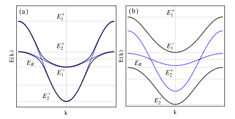
Figure 1: Two situations of clean energy dispersions. The dashed and solid curves correspond to decoupled and coupled chains. The decoupled dispersion curves intersect at the resonance energy $E_{R}$. (a) no gap: $E_{1}^{-}\leq E_{2}^{+}$. There are two propagating channels at a given energy for $E_{1}^{-}\leq E\leq E_{2}^{+}$. (b) gapped: $E_{1}^{-}>E_{2}^{+}$. Apart from a forbidden band, only one propagating channel exists.

According to Eq. (II.1.1), there are two cases of energy dispersions, which may arise depending on the choice of parameters:

(i) In the case of $E_{1}^{-}\leq E_{2}^{+}$ [see Fig. 1(a)], there is no gap between the two bands. This is the case if the detuning $\delta e$ and the interchain coupling $t$ are both not too large. More precisely, one needs $|\delta e|<2(t_{1}+t_{2})$ and $t\leq t_{c}$, where

$$t_{c}=\frac{\sqrt{t_{1}t_{2}\left[4\left(t_{1}+t_{2}\right)^{2}-\delta{e}^{2}\right]}}{t_{1}+t_{2}}.$$ (17)

In the energy interval $E_{1}^{-}\leq E\leq E_{2}^{+}$, we have two propagating channels; otherwise, at most one propagating channel exists.

(ii) In the opposite case, $E_{1}^{-}>E_{2}^{+}$ [see Fig. 1(b)], there is a gap between the two bands. We therefore have at most one propagating channel at any energy.

Moreover, if $k_{\tau}$ is the wavevector of a propagating channel, we call $k_{\tau}\in(-\pi,\pi]$, and $k_{\tau}\geq 0$ and $k_{\tau}<0$ the right- and left-moving branch, resp. From Eq. (14) we also define a rapidity for each propagating channel as

$$v_{\tau}\equiv\left|\frac{\partial{\lambda_{\tau}}}{{\partial{k_{\tau}}}}\right|=\sqrt{4-\lambda_{\tau}^{2}}.$$ (18)

II.1.2 Disordered part

The impurity matrix (9) contains two ingredients which determine the localization properties of the model. One is ${\epsilon}_{x\pm}$ [see Eq. (11)], which are the equally weighted (either symmetric or anti-symmetric) combinations of effective disorder on the two legs. The other is the mixing angle $\gamma$ [see Eq. (12)], which describes the effective coupling between the two legs. We refer to $\gamma$ as the bare mixing angle because it will be renormalized by disorder. The renormalized mixing angle $\tilde{\gamma}$ [see Eq. (103)] will be discussed in Sec. IV. Being functions of these two quantities, the diagonal elements of $\tilde{\boldsymbol{{\epsilon}}}_{x}$ are local random potentials applied on the two channels $\tau=1,2$, and the off-diagonal elements describe the random hopping between them.

We analyze the model qualitatively in terms of effective disorder and bare mixing angle before carrying out the detailed calculation. As already discussed above, either one or two propagating channels are permitted at a given energy. This leads to two distinct mechanisms of localization in the bulk of the energy band:

(i) Two-channel regime. In this case, the physics is dominated by the mixing angle $\gamma$. If $\gamma\sim 0$ or $\pi$, the mixing of the two channels is weak: The magnitudes of off-diagonal elements of matrix  (9) are much smaller than the magnitudes of the diagonal elements. This means that the two legs are weakly entangled, and the transverse hopping $t$ can be treated as a perturbation. A perturbative study of wavefunctions in this regime is presented in Sec. VII. However, if $\gamma\sim\pi/2$, the magnitudes of the off-diagonal elements are of the same order as the diagonal elements. This implies that the two legs are strongly entangled. The localization properties are controlled by the leg with strong disorder, because in Eq. (11) it always dominates over the weaker disorder on the other leg.

(ii) One-channel regime. The single-channel case has been solved by Berezinskiiberez and Mel’nikovmel in the case of a single chain. The results they obtained can be applied in our problem by substituting the variance of disorder and rapidity of the propagating channel with the corresponding quantities. However, we have to emphasize here that even if only one channel exists, coupling effects still present, since both the effective disorder and the rapidity in the remaining channel depend on the transport properties of both legs. In the one-channel regime the second channel is still present, but supports only evanescent modes. We show in Sec. VI that the effect of the evanescent channel on the propagating one is subleading when disorder is weak.

II.2 Transfer matrix approach

The Fokker-Planck approach and its related notations, such as the transfer matrix, the S-matrix etc. are introduced in detail in Refs. mpk1, and mpk2, . We only outline the methodology here. The Fokker-Planck approach to one- or quasi-one dimensional systems with static disorder at zero temperature is based on studying the statistical distribution of random transfer matrices for a system of finite length. An ensemble of such transfer matrices is constructed by imposing appropriate symmetry constraints. In the present model there are two underlying symmetries: time-reversal invariance and current conservation, which dramatically reduce the number of free parameters of transfer matrices. After a proper parametrization, the probability distribution function of these parameters completely describes the ensemble of transfer matrices, and therefore totally determines the statistical distributions of many macroscopic quantities of the system, such as the conductance, etc. In order to obtain the probability distribution function of the free parameters, a stochastic evolution-like procedure is introduced by computing the variation of the probability distribution function of these parameters in a “bulk” system as an extra impurity “slice” is patched on one of its terminals, under the assumption that the patched slice is statistically independent of the bulk. Thereby, we construct a Markovian process for the probability distribution function. This is described by a kind of Fokker-Planck equation in the parameter space of the transfer matrix with the length of the system as the time variable. Essentially, this procedure is analogous to deriving the diffusion equation from the Langevin equation for a Brownian particle. In practice, taking the length to infinity, we can analytically extract asymptotic properties of the model, such as localization lengths, etc., from the fixed point solution of the Fokker-Planck equation.

As discussed above, the only microscopic quantity needed in order to write down the Fokker-Planck equation of our model Hamiltonian (1) is the transfer matrix of an “elementary slice” at any co-ordinate $x$. The Schrödinger equation (7) can be represented in the following “transfer-matrix” form:

$$\tilde{\Phi}(x+1)=\tilde{\mathbf{m}}_{x}\tilde{\Phi}(x),$$ (19)

where the $4$-component wave function $\tilde{\Phi}(x)$ and the $4\times 4$ transfer matrix $\tilde{\mathbf{m}}_{x}$ is explicitly shown in the $2\times 2$ “site-ancestor site” form:

$$\tilde{\Phi}(x)\equiv\begin{pmatrix}\tilde{\Psi}(x)\\ \tilde{\Psi}(x-1)\end{pmatrix},\quad\tilde{\mathbf{m}}_{x}\equiv\begin{pmatrix}\tilde{\mathbf{h}}+\tilde{\boldsymbol{\epsilon}}_{x}&-\mathbf{1}\\ \mathbf{1}&\mathbf{0}\end{pmatrix}.$$ (20)

with $\tilde{\Psi}(x)$ and $\tilde{\bf{h}}$, $\tilde{\boldsymbol{\epsilon}}_{x}$ being the $2$-component vector and $2\times 2$ matrices in the space of channels as defined in Eq. (7).

The transfer matrix $\tilde{\mathbf{m}}_{x}$ is manifestly real (which reflects the time-reversal symmetry) and symplectic (which reflects the current conservation):

$$\tilde{\bf m}_{x}^{T}J\tilde{\bf m}_{x}=J,$$ (21)

where $J$ is the standard skew-symmetric matrix:

$$J=\left(\begin{matrix}0&\mathbf{1}\cr-\mathbf{1}&0\end{matrix}\right).$$ (22)

Note, however, that the transfer matrix $\tilde{\mathbf{m}}_{x}$ is not a convenient representation to construct a Fokker-Planck equation. The reason is simple: because it is not diagonal without impurities, the perturbative treatment of impurities is hard to perform. The proper transfer matrix $\mathbf{m}_{x}$ is a certain rotation, which does not mix the two channels of the matrix $\tilde{\mathbf{m}}_{x}$, but transforms to a more convenient basis within each 2-dimensional channel subspace [see Appendix A]. The latter corresponds to the basis of solutions to the disorder-free Schrödinger equation $\psi_{\tau}(x)$ ($\tau=1,2$ labeling the channels) which conserves the current along the ladder:

$$j_{x}=-i\,[\psi_{\tau}^{*}(x)\psi_{\tau}(x+1)-h.c.]={\rm const}=\pm 1.$$ (23)

For propagating modes with real wave vectors $k_{\tau}$ these are the right- and left- moving states

$$\psi_{\tau}^{\pm}(x)=e^{\pm ik_{\tau}\,x}/\sqrt{2\sin k_{\tau}},$$ (24)

which obey the conditions:

$$\psi_{\tau}^{\pm}(x)=(\psi_{\tau}^{\pm}(-x))^{*}.$$ (25)

For the evanescent modes with imaginary $k=i\kappa$ the corresponding current-conserving states obeying Eq. (25) can be defined, too:

$$\psi_{\tau}^{\pm}(x)=\frac{{\rm exp}[\mp i\pi/4-\kappa_{\tau}x]+{\rm exp}[\pm i\pi/4+\kappa_{\tau}x]}{\sqrt{4\sinh\kappa_{\tau}}}$$ (26)

In this new basis of current-conserving states, the transfer matrix takes the form (see Appendix A):

$$\mathbf{m}_{x}=\mathbf{1}+\delta\mathbf{m}_{x},\quad\delta\mathbf{m}_{x}=\begin{pmatrix}-i\boldsymbol{\alpha}_{x}^{\ast}\tilde{\boldsymbol{{\epsilon}}}_{x}\boldsymbol{\alpha}_{x}&-i\boldsymbol{\alpha}_{x}^{\ast}\tilde{\boldsymbol{{\epsilon}}}_{x}\boldsymbol{\alpha}_{x}^{\ast}\\ \,\,i\boldsymbol{\alpha}_{x}\tilde{\boldsymbol{{\epsilon}}}_{x}\boldsymbol{\alpha}_{x}&\,\,i\boldsymbol{\alpha}_{x}\tilde{\boldsymbol{{\epsilon}}}_{x}\boldsymbol{\alpha}_{x}^{\ast}\end{pmatrix},$$ (27)

where the matrix $\boldsymbol{\alpha}_{x}$ is diagonal in channel space,

$$\boldsymbol{\alpha}_{x}=\text{diag}\left(\psi_{1}^{+}(x),\psi_{2}^{+}(x)\right)_{{\rm ch}}.$$ (28)

Note that it is expressed in terms of the two components of the current conserving states Eqs. (24, 26) corresponding to the first and the second channel.

In Eq. (27), the unit matrix $\mathbf{1}$ is the pure part of $\mathbf{m}_{x}$, which keeps the two incident plane waves invariant, and $\delta\mathbf{m}_{x}$ describes the impurities, which break the momentum conservation and induce intra- and inter-channel scattering. The physical meaning of $\mathbf{m}_{x}$ can be understood from the scattering processes described below. If there is only one right-moving plane wave in the 1-channel on the left-hand side (l.h.s.) of the slice, which is represented by a four dimensional column vector with the first component one and the others zero, we can detect four components on the right-hand side (r.h.s.) of the slice, including the evanescent modes. In the case of two propagating channels these four components are right- and left-moving plane waves in the 1- and 2-channel, whose magnitudes and phase-shifts form the first row of $\mathbf{m}_{x}$. The other rows can be understood in the same manner. In short, the $11$-, $12$-, $21$- and $22$- block of $\delta\mathbf{m}_{x}$ represent respectively the right-moving forward-scattering, right-moving backward-scattering, left-moving backward-scattering and left-moving forward-scattering on the slice. In each block, the diagonal elements represent intra-channel scattering and the off-diagonal elements represent inter-channel scattering.

It is important that $\mathbf{m}_{x}$, Eq. (27), fulfills the same constraints regardless of the propagating or evanescent character of the modes [see Appendix A]:

$$\mathbf{m}_{x}^{\ast}=\boldsymbol{\varSigma}_{1}\mathbf{m}_{x}\boldsymbol{\varSigma}_{1},\quad\mathbf{m}_{x}^{\dagger}\boldsymbol{\varSigma}_{3}\mathbf{m}_{x}=\boldsymbol{\varSigma}_{3},$$ (29)

where $\boldsymbol{\varSigma}_{1}$ and $\boldsymbol{\varSigma}_{3}$ are the four dimensional generalization of the first and third Pauli matrix with zero and unit entries replaced by $2\times 2$ zero and unit matrices in the channels space. The first condition follows from $\tilde{\bf m}_{x}^{\ast}=\tilde{\bf m}_{x}$, while the second condition is a consequence of the symplecticity Eq. (21). Thus these conditions are a direct consequence of the fact that $\tilde{\bf m}_{x}$ belongs to the symplectic group $\text{Sp}(4,\mathbb{R})$. As is obvious from the choice of the basis (23-26), their physical meaning is the time-reversal symmetry and the current conservation.

The representation Eq. (27) of the transfer matrix of an “elementary slice” renders both the physical interpretation and the symmetry constraints very transparent, and it will be seen to be a convenient starting point to construct the Fokker-Planck equation. On the other hand, since $\tilde{\mathbf{m}}_{x}$ [see Eq. (20)] is real and has a relatively simple form, it is more suitable for numerical calculations.

III fokker-planck equation for the distribution function of parameters

III.1 Parametrization of transfer matrices

Once the “building block” (27) is worked out, we can construct the Fokker-Planck equation by the blueprint of the Fokker-Planck approach.mel ; dorok ; mpk1 ; mpk2 The transfer matrix of a disordered sample with length $L$ is

$$\mathbf{M}(L)=\prod_{x=1}^{L}\mathbf{m}_{x}=\mathbf{m}_{L}\cdot\mathbf{m}_{L-1}\cdots\mathbf{m}_{1},$$ (30)

which is a $4\times 4$ complex random matrix. It is easy to verify that $\mathbf{M}(L)$ also satisfies the time reversal invariance and current conservation conditions (29). It has been proved in Ref. mpk1, that all the $4\times 4$ matrices satisfying Eq. (29) form a group which is identified with the symplectic group $\text{Sp}(4,\mathbb{R})$. By the Bargmann’s parametrization of $\text{Sp}(4,\mathbb{R})$,mpk2 one can represent $\mathbf{M}(L)$ as

$$\mathbf{M}=\begin{pmatrix}\mathbf{u}&0\\ 0&\mathbf{u}^{\ast}\end{pmatrix}\begin{pmatrix}\sqrt{\frac{\mathbf{F}+\mathbf{1}}{2}}&\sqrt{\frac{\mathbf{F}-\mathbf{1}}{2}}\\ \sqrt{\frac{\mathbf{F}-\mathbf{1}}{2}}&\sqrt{\frac{\mathbf{F}+\mathbf{1}}{2}}\end{pmatrix}\begin{pmatrix}\tilde{\mathbf{u}}&0\\ 0&\tilde{\mathbf{u}}^{\ast}\end{pmatrix},$$ (31)

where $\mathbf{u}$ and $\tilde{\mathbf{u}}$ are elements of the unitary group $\text{U}(2)$, and statistically independent from each other, and

$$\mathbf{F}=\text{diag}(F_{1},F_{2}),$$ (32)

with $F_{\varrho}\in[1,\infty)$ and $\varrho\in\{1,2\}$. Because $\text{U}(2)$ hamsh has four real parameters, the group $\text{Sp}(4,\mathbb{R})$ has ten real parameters. Furthermore, it is convenient to parametrize a $\text{U}(2)$ matrix by three Euler angles and a total phase angle, i.e.,

$$\mathbf{u}(\phi,\varphi,\theta,\psi)=e^{-i\frac{\phi}{2}}e^{-i\frac{\varphi}{2}\hat{\sigma}_{3}}e^{-i\frac{\theta}{2}\hat{\sigma}_{2}}e^{-i\frac{\psi}{2}\hat{\sigma}_{3}},$$ (33)

in which $\hat{\sigma}_{2}$ and $\hat{\sigma}_{3}$ are the second and third Pauli matrix, and the four angles take their values in the range $\phi,\varphi\in[0,2\pi)$, $\theta\in[0,\pi)$ and $\psi\in[0,4\pi)$. In matrix form in the channels space, $\mathbf{u}$ can be written as

$$\mathbf{u}=e^{-i\frac{\phi}{2}}\begin{pmatrix}\cos{\frac{\theta}{2}}e^{-\frac{i}{2}(\varphi+\psi)}&-\sin{\frac{\theta}{2}}e^{-\frac{i}{2}(\varphi-\psi)}\\ \sin{\frac{\theta}{2}}e^{\frac{i}{2}(\varphi-\psi)}&\cos{\frac{\theta}{2}}e^{\frac{i}{2}(\varphi+\psi)}\end{pmatrix}_{{\rm ch}},$$ (34)

which is convenient for the perturbative calculation below. The $\text{U}(2)$ matrix $\tilde{\mathbf{u}}$ can be parametrized independently in the same form as Eq. (34).

The probability distribution function of these ten real parameters determines completely the transfer matrix ensemble of the ladder described by the Hamiltonian  (1). The goal of the Fokker-Planck approach is to obtain the Fokker-Planck equation satisfied by this probability distribution function, in which the role of time is played by the length $L$.

From Eq. (31) we obtain the transmission matrix

$$\mathbf{t}:=(M_{++}^{\dagger})^{-1}=\mathbf{u}\left(\frac{\mathbf{F}+\mathbf{1}}{2}\right)^{-1/2}\tilde{\mathbf{u}},$$ (35)

by a simple relation between the transfer matrix and its corresponding S-matrix.mpk1 ; mpk2 ; imp-trassm-mat Due to the unitarity of $\tilde{\mathbf{u}}$, the transmission co-efficients of the two channels are the two eigenvalues of the Hermitian matrix

$$\mathbf{T}=\mathbf{t}\mathbf{t}^{\dagger}=\mathbf{u}\left(\frac{\mathbf{F}+\mathbf{1}}{2}\right)^{-1}\mathbf{u}^{\dagger},$$ (36)

which are

$$T_{\varrho}=\frac{2}{F_{\varrho}+1},$$ (37)

where $\varrho\in\{1,2\}$ is the index of the two-dimensional eigenspace of the matrix $\mathbf{T}$. Now the physical meaning of the parametrization (31) becomes clear. The $F_{\varrho}$’s are related to the two transmission co-efficients by the simple form Eq. (37). The matrix $\mathbf{u}$ diagonalizing the matrix $\mathbf{T}$, contains the two eigenvectors of $\mathbf{T}$, describing the polarization of the plane wave eigenmodes incident from the l.h.s. of the sample. For instance, if $\theta=0$ ($\mathbf{u}$ is a diagonal matrix of redundant phases), the two channels do not mix, and the incident waves are fully polarized in the basis of channels. On the other hand, if $\theta=\pi$, the two channels are equally mixed, and the incident waves are unpolarized. In analogy to spherical co-ordinates, we will refer to the $F_{\varrho}$’s as the radial variables, while the angles in $\mathbf{u}$ or $\tilde{\mathbf{u}}$ are called angular variables.

In principle, using the “building block” (27) and the parametrization (31), we can solve the full problem by writing down a Fokker-Planck equation for the joint probability distribution function of all the ten parameters of $\mathbf{M}$. However, since we are merely interested in the transmission co-efficients which are determined by the probability distribution function of $\mathbf{T}$, instead of manipulating $\mathbf{M}$, we study

$$\begin{split}\mathbf{R}&=\mathbf{M}\mathbf{M}^{\dagger}\\ &\\ &=\begin{pmatrix}\mathbf{u}&0\\ 0&\mathbf{u}^{\ast}\end{pmatrix}\begin{pmatrix}\mathbf{F}&\sqrt{\mathbf{F}^{2}-\mathbf{1}}\\ \sqrt{\mathbf{F}^{2}-\mathbf{1}}&\mathbf{F}\end{pmatrix}\begin{pmatrix}\mathbf{u}^{\dagger}&0\\ 0&\mathbf{u}^{\text{T}}\end{pmatrix}.\end{split}$$ (38)

$\mathbf{R}$ is a Hermitian matrix and contains only six parameters:

$$\vec{\lambda}(\mathbf{R})=(F_{1},F_{2},\theta,\psi,\phi,\varphi).$$ (39)

The probability distribution function of $\vec{\lambda}$, denoted by $P_{L}(\vec{\lambda})$, determines the transmission properties of the sample with length $L$. $P_{L}(\vec{\lambda})$ is defined by

$$P_{L}(\vec{\lambda})=\overline{\delta{\left(\vec{\lambda}-\vec{\lambda}{\left(\mathbf{R}(L)\right)}\right)}},$$ (40)

where the overline denotes the average over realizations of the random potentials in the sample. It is convenient to introduce the characteristic function of $P_{L}(\vec{\lambda})$

$$\tilde{P}_{L}(\vec{p})=\int{d\vec{\lambda}e^{i\vec{p}\cdot\vec{\lambda}}P_{L}(\vec{\lambda})}=\overline{e^{i\vec{p}\cdot\vec{\lambda}{\left(\mathbf{R}(L)\right)}}}.$$ (41)

Our main goal in this paper is to calculate the two localization lengths, defined as the inverse Lyapunov exponents of the transfer matrix (31):

$$\xi_{1(2)}^{-1}\equiv-\lim_{L\rightarrow\infty}{\frac{1}{2}\frac{d}{dL}\langle\ln{T_{\max(\min)}}\rangle_{L}},$$ (42)

in which the subscripts “max” and “min” denote the larger and smaller of the two real values $T_{1,2}$, and the averaging $\langle\cdot\rangle_{L}$ is earned out with the probability distribution $P_{L}(\vec{\lambda})$. Therefore, by definition

$$\xi_{1}>\xi_{2}.$$ (43)

III.2 Physical interpretation of $\xi_{1}$ and $\xi_{2}$

It is worthwhile to visualize how two parametrically different localization lengths ($\xi_{1}\gg\xi_{2}$) manifest themselves in transport properties. For instance, let us discuss the dimensionless conductance $\text{g}=T_{1}+T_{2}$, a typical behavior of which is shown as a function of the sample length $L$ in Fig. 2. If $L\ll\xi_{2}$, $T_{\varrho}\approx 1$, and $\text{g}\approx 2$ corresponds to a nearly perfect transmission. As $L$ increases, $T_{\varrho}$ and g decay exponentially. $T_{2}$ decays much faster than $T_{1}$ since $\xi_{1}\gg\xi_{2}$. As long as $L<\xi_{1}$ the system still conducts well since g is still appreciable. For $L\sim\xi_{1}$ it crosses over to an insulating regime. On the other hand, $\xi_{2}$ marks the crossover length scale below which $\text{g}(L)$ (black curve) decreases as fast as $T_{2}$ (blue dashed curve) until the conductance saturates to a plateau $\text{g}\approx 1$. For $L>\xi_{2}$, g decays with the slow rate $\xi_{1}^{-1}$, like $T_{1}$ (red dotted curve). Therefore, the two parametrically different localization lengths can be identified by two distinct decay rates of g at small and large length scales.

The statistics of transmission eigenvalues and localization lengths of disordered multi-channel micro-waveguides have been visualized in experiments .shi-gen However, only more or less isotropically disordered cases (identical hopping and disorder strength in each channel) were realized, while a situation where $\xi_{1}\gg\xi_{2}$ is hard to achieve in such systems (see Ref. shi-gen, and references therein). In contrast such anisotropic situations are rather natural in exciton polariton systems.

We will see in Sec. VII that the two localization lengths $\xi_{1}$ and $\xi_{2}$ also characterize the spatial variations of the eigenfunctions $\Psi(x)$ on the two legs.

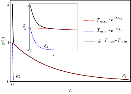
Figure 2: Schematic diagram for typical values of dimensionless conductance g as a function of the length $L$ in the case $\xi_{1}\gg\xi_{2}$. A crossover happens at $L\sim\xi_{2}$. In the region $L<\xi_{2}$, g decays as fast as $T_{\text{min}}$ (see the insert). Once $L>\xi_{2}$, g decays as slowly as $T_{\text{max}}$. The system is well conducting if $L<\xi_{1}$ and crosses to an insulating regime for $L>\xi_{1}$.

III.3 Fokker-Planck equation for the distribution function of $\vec{\lambda}(\mathbf{R})$

Having a disordered sample of length $L$, whose transfer matrix is $\mathbf{M}(L)$ and adding one more slice, we obtain the transfer matrix of the sample with length $L+1$:

$$\mathbf{M}(L+1)=\mathbf{m}_{L+1}\mathbf{M}(L).$$ (44)

Simultaneously, according to Eqs. (38) and (27), $\mathbf{R}(L)$ is updated to

$$\mathbf{R}(L+1)=\mathbf{m}_{L+1}\mathbf{R}(L)\mathbf{m}_{L+1}^{\dagger}=\mathbf{R}(L)+\delta{\mathbf{R}},$$ (45a)

$$\delta{\mathbf{R}}=(\mathbf{R}\delta{\mathbf{m}^{\dagger}_{L+1}}+h.c.)+\delta{\mathbf{m}_{L+1}}\mathbf{R}\delta{\mathbf{m}^{\dagger}_{L+1}}.$$ (45b)

Accordingly, $\vec{\lambda}{\left(\mathbf{R}(L)\right)}$ is incremented by

$$\vec{\lambda}{\left(\mathbf{R}(L+1)\right)}=\vec{\lambda}{\left(\mathbf{R}(L)\right)}+\delta{\vec{\lambda}}.$$ (46)

According to Eqs. (41) and (46), we obtain the characteristic function of $P_{L+1}(\vec{\lambda})$:

$$\tilde{P}_{L+1}(\vec{p})=\overline{e^{i\vec{p}\cdot\vec{\lambda}{\left(\mathbf{R}(L+1)\right)}}}=\overline{e^{i\vec{p}\cdot\vec{\lambda}{\left(\mathbf{R}(L)\right)}}e^{i\vec{p}\cdot\delta{\vec{\lambda}}}}.$$ (47)

We can expand $e^{i\vec{p}\cdot\delta{\vec{\lambda}}}$ on the r.h.s. of Eq. (47) into a Taylor series $e^{i\vec{p}\cdot\delta{\vec{\lambda}}}=\sum_{n}^{\infty}{(i\vec{p}\cdot\delta{\vec{\lambda}})^{n}}$. Using Eqs. (45,46) standard perturbation theory yields an expansion of $\delta{\vec{\lambda}}$ in powers of the disorder potential as $\delta{\vec{\lambda}}=\sum_{n\geq 1}\delta{\vec{\lambda}}^{(n)}$, where $\delta{\vec{\lambda}}^{(n)}$ is of $n$-th order in $\tilde{\boldsymbol{\epsilon}}$. With this, the r.h.s. of Eq. (47) can be expanded in powers of the disorder potential. In principle, we can proceed with this expansion to arbitrarily high orders. Thereafter, the average over disorder on the slice $L+1$ can be performed. Eqs. (45)-(47) fully define our problem. However, it is impossible to solve it analytically without further simplification.

Progress can be made by considering the weak disorder limit. In the two-channel regime, the weak disorder limit implies that both of the mean free paths are much larger than the lattice constant. As a first estimation, applying the Born approximation to an “elementary slice”, the inverse mean free paths of the two propagating channels can be expressed as certain linear combinations of the variances of the effective disorders on the two chains, defined as

$$\chi^{2}_{\nu}=\frac{\sigma^{2}_{\nu}}{t_{\nu}^{2}}.$$ (48)

for chain $\nu$. In the weak disorder limit where the smaller of the two localization lengths is much larger than the lattice constant,

$$l\gg 1,$$ (49)

only the terms proportional to $\chi^{2}_{\nu}$ on the r.h.s of Eq. (47) have to be taken into account. Hence, we calculate $\delta{\vec{\lambda}}$ perturbatively up to the second order [see Appendix B]. If $L\gg 1$, as we always assume, $\tilde{P}_{L+1}-\tilde{P}_{L}\simeq\partial_{L}{\tilde{P}_{L}}$. Under these conditions, Eq. (47) leads to

$$\partial_{L}{\tilde{P}_{L}}=\overline{i\vec{p}\cdot\delta{\vec{\lambda}}^{(2)}e^{i\vec{p}\cdot\vec{\lambda}{\left(\mathbf{R}(L)\right)}}}-\frac{1}{2}\overline{\left(\vec{p}\cdot\delta{\vec{\lambda}}^{(1)}\right)^{2}e^{i\vec{p}\cdot\vec{\lambda}{\left(\mathbf{R}(L)\right)}}}.$$ (50)

Note that because the random potentials in different slices are uncorrelated, the $\delta{\vec{\lambda}}^{(n)}$ terms can be averaged independently of $e^{i\vec{p}\cdot\vec{\lambda}{\left(\mathbf{R}(L)\right)}}$. By the inverse of the Fourier transform defined in Eq. (41) we obtain the Fokker-Planck equation for $P_{L}(\vec{\lambda})$:

$$\partial_{L}{P}=-\sum_{i=1}^{6}{\partial_{\lambda_{i}}\left[{\overline{\delta{\lambda_{i}^{(2)}}}P}-\frac{1}{2}\sum_{j=1}^{6}{\partial_{\lambda_{j}}{\left(\overline{\delta{\lambda_{i}^{(1)}}\delta{\lambda_{j}^{(1)}}}P\right)}}\right]}.$$ (51)

In Eq. (51) the averages are taken over the realizations of random potentials in the slice at $L+1$.

The Fokker-Planck equation (51) can be rewritten in the form of a continuity equation:

$$\partial_{L}{P}=-\sum_{i=1}^{6}{\partial_{\lambda_{i}}J_{i}},$$ (52)

where the generalized current density $J_{i}$ takes the form:

$$J_{i}={\text{v}_{i}(\vec{\lambda})P}-\sum_{j=1}^{6}D_{ij}(\vec{\lambda})\partial_{\lambda_{j}}{P},$$ (53)

with

$$\text{v}_{i}(\vec{\lambda})=\overline{\delta{\lambda_{i}^{(2)}}}+\partial_{\lambda_{j}}D_{ij}(\vec{\lambda}),$$ (54a)

$$D_{ij}(\vec{\lambda})=\frac{1}{2}\overline{\delta{\lambda_{i}^{(1)}}\delta{\lambda_{j}^{(1)}}}.$$ (54b)

$\text{v}_{i}(\vec{\lambda})$ and $D_{ij}(\vec{\lambda})$ are a generalized stream velocity and a generalized diffusion tensor, respectively.

In order to solve Eq. (51), we have to add the initial condition, namely, $P_{0}(\vec{\lambda})$. Usually $P_{0}(\vec{\lambda})$ is chosen as the probability distribution function in the ballistic limit,bee

$$P_{0}(\vec{\lambda})=\delta{(F_{1}-1)}\delta{(F_{2}-1)}\delta{(\theta)}\delta{(\phi)}\delta{(\psi)}\delta{(\varphi)},$$ (55)

where $\delta(x)$ is the Dirac delta function. However, as we will see later, a unique fixed point of $P_{L}(\vec{\lambda})$ exists in the limit $L\rightarrow\infty$, which does not depend upon the initial condition. Essentially, the existence of a fixed-point solution of Eq. (51) is protected by Anderson localization which prevents the system from chaos. fgp

III.4 Coarsegraining

Let us analyze the r.h.s. of Eq. (51) qualitatively. From Eqs. (178) and (180) in the Appendix, it is clear that the co-efficients $\overline{\delta{\lambda_{i}^{(1)}}\delta{\lambda_{j}^{(1)}}}$ and $\overline{\delta{\lambda_{i}^{(2)}}}$ are sums of terms carrying phase factors $1,e^{\pm i(k_{1}-k_{2})L},...$ and so on. These phase factors come from the disorder average of products of two elements of the matrices (27). Their phases correspond to the possible wave vector transfers of two scatterings from a slice, similarly as found in the Berezinskii technique berez . They are thus linear combinations of two or four values of $\pm k_{1,2}$:

$${\bf K}_{\rm osc} = \left\{\,\pm\Delta{k},\quad\pm 2\Delta{k},\right.$$

$$\quad\pm 2k_{1(2)},\quad\pm(k_{1}+k_{2}),\quad\pm\left[3k_{1(2)}-k_{2(1)}\right],$$

$$\quad\left.\pm 4k_{1(2)},\quad\pm 2(k_{1}+k_{2}),\quad\pm\left[3k_{1(2)}+k_{2(1)}\right]\right\},$$

where

$$\Delta{k}=k_{1}-k_{2}.$$ (57)

Terms with phase “$0$” do not oscillate. The largest spatial period of the oscillating terms is

$$L_{\rm osc}=\max_{\delta k\in{\bf K}_{\rm osc}}\delta k^{-1}$$ (58)

Under the condition that

$$L_{\rm osc}\ll l,$$ (59)

a coarsegrained probability distribution function can be defined as the average of $P_{L}(\vec{\lambda})$ over $L_{\rm osc}$. From now on, we use the same symbol $P_{L}(\vec{\lambda})$ to denote its coarsegrained counterpart, which satisfies Eq. (51), but neglecting the oscillating terms.

Additionally, at special energies it may happen that an oscillation period becomes commensurate with the lattice spacing , $\delta k=\pi/n$. An important example of this commensurability is the situation where $\delta{e}=0$, $2(k_{1}+k_{2})=2\pi$ at $E=0$. In this case the terms with the phase factor $e^{\pm 2i(k_{1}+k_{2})L}$ do not average and give anomalous contributions to the non-oscillating co-efficients. This effect leads to the so-called center-of-band anomaly in the eigenfunction statistics of the one-chain Anderson model (see Ref. krav-yud, and references therein). While they are not included in our analytical study, the commensurability-induced anomalies can be seen clearly in the numerical results for localization lengths (cf. Figs. 6, 7, 10 and 11).

The coarsegraining procedure leads to a significant simplification: the co-efficients on the r.h.s. of Eq. (51) do not depend on $L$, $\phi$ and $\varphi$ any longer, which renders the solution of Eq. (51) much easier. Its non-oscillating co-efficients are evaluated in Appendix B. We do not reproduce them explicitly here, since we further transform the Fokker Planck equation below. However it is worthwhile pointing out a formal property of its co-efficients. From Eqs. (176), (178) and (180), it is easy to see that the ingredients for evaluating $\overline{\delta{\lambda_{i}^{(1)}}\delta{\lambda_{j}^{(1)}}}$ and $\overline{\delta{\lambda_{i}^{(2)}}}$ are the disorder-averaged correlators between any two elements of matrices (27). During the calculation, three Born cross sections appear naturally, being covariances of the effective disorder variables,

$$V_{1}=\frac{1}{4v_{1}^{2}}\left(\chi^{2}_{1}\cos^{4}{\frac{\gamma}{2}}+\chi^{2}_{2}\sin^{4}{\frac{\gamma}{2}}\right),$$ (60a)

$$V_{2}=\frac{1}{4v_{2}^{2}}\left(\chi^{2}_{1}\sin^{4}{\frac{\gamma}{2}}+\chi^{2}_{2}\cos^{4}{\frac{\gamma}{2}}\right),$$ (60b)

$$V_{3}=\frac{1}{4v_{1}v_{2}}\left(\chi^{2}_{1}+\chi^{2}_{2}\right)\sin^{2}{\frac{\gamma}{2}}\cos^{2}{\frac{\gamma}{2}},$$ (60c)

in which $V_{1(2)}$ corresponds to intra-channel scattering processes $k_{1(2)}\leftrightarrow-k_{1(2)}$, and $V_{3}$ corresponds to inter-channel scattering processes $k_{1(2)}\leftrightarrow\pm k_{2(1)}$. Note that the effective disorder variances (48) enter into the three Born cross-sections, instead of the bare variances (2). We will see that the above three Born cross-sections completely define the localization lengths and most phenomena can be understood based on them.

We note that the coarsegraining, through Eq. (59), imposes a crucial restriction on the applicability of the simplified Fokker-Planck equation. According to Eqs. (II.1.1) and (14), if $t$ is small enough, at $E=E_{R}$,

$$|\Delta{k}|\propto t.$$ (61)

In this case, Eqs. (59) and (61) require that

$$t\gg\delta{E},$$ (62)

where

$$\delta{E}\propto l^{-1},$$ (63)

is the characteristic disorder energy scale (essentially the level spacing in the localization volume). In other words, Eq. (62) imposes a “strong coupling” between the two legs, as compared with the disorder scale. However, from the point of view of the strength of disorder, Eq. (62) is a more restrictive condition than $\xi_{2}\gg 1$ on the smallness of disorder. However, it is automatically fulfilled in the limit $\sigma_{\nu}\rightarrow 0$ at fixed values of coupling constants $t$ and $t_{\nu}$.

Eq. (62) restricts the region of applicability of the simplified equation (68) which we will derive below. Indeed, we will see that by simply taking the limit $t\rightarrow 0$ in the solution of that equation one does not recover the trivial result for the uncoupled chains. This is because the equation is derived under the condition that $t$ is limited from below by Eq. (62). The “weak coupling” regime is studied numerically in Sec. V.1 and the cross-over to the limit of uncoupled chains is observed at a scale of $t\sim l^{-1}$ as expected.

Since the definition of localization lengths (42) only involves the $F_{\varrho}$’s, and since the co-efficients of Eq. (51) do not contain $\phi$ and $\varphi$, we define the marginal probability distribution function

$$W_{L}(F_{1},F_{2},\theta,\psi)=\int{{d\phi}{d\varphi}P_{L}(\vec{\lambda})}.$$ (64)

Further we change variables to the set

$$\vec{\eta}=(F_{1},F_{2},u,\psi),$$ (65)

where

$$u=\cos{\theta},\quad u\in(-1,1].$$ (66)

We thus have

$$W_{L}(\vec{\eta})=\int{d\phi d\varphi P_{L}(F_{1},F_{2},\theta(u),\psi,\phi,\varphi)}.$$ (67)

Substituting Eq. (67) into (51), and replacing the differential operators $\partial_{\theta}\rightarrow-\sqrt{1-u^{2}}\partial_{u}$ and $\partial_{\theta}^{2}\rightarrow-u\partial_{u}+(1-u^{2})\partial_{u}^{2}$, we obtain the Fokker-Planck equation for $W_{L}(\vec{\eta})$:

$$\partial_{L}{W}=\sum_{i=1}^{4}{\left[\partial_{\eta_{i}}\left(c_{ii}\partial_{\eta_{i}}W\right)+\partial_{\eta_{i}}\left(c_{i}W\right)\right]}+\sum_{j>i=1}^{4}{\partial_{\eta_{i}}\partial_{\eta_{j}}\left(c_{ij}W\right)}.$$ (68)

The co-efficients $c_{i},c_{ij}$ are relatively simple functions of $\vec{\eta}$. They can be obtained from the averages of the matrix elements computed in App. B, and are given in App. C. However, only a small number of them will turn out to be relevant for the quantities of interest to us.

One can see that in Eq. (68) the radial variables, $F_{\varrho}$, are entangled with the angular variables $u$ and $\psi$. Thus Eq. (68) is more general than the canonical DMPK equationdorok ; mpk1 ; mpk2 where only radial variables appear. To emphasize the difference we refer to Eq. (68) as the extended DMPK equation. The derivation of Eq. (68) for the two-leg problem is our main technical achievement in the present paper. It allows us to obtain the evolution (as a function of $L$) of the expectation value of any quantity defined in $\vec{\eta}$-space.

IV Calculating the localization length

It is well-known that in quasi-one dimensional settings single particles are always localized at any energy in arbitrarily weak (uncorrelated) disorder. abra-and-Licc-rama The localization length quantifies the localization tendency in real space. In this section we calculate the localization lengths for the present model.

The analytic expression of $\ln{T_{\max(\min)}}$ in Eq. (42) can be written as

$$\ln{T_{\max(\min)}}=\Theta(\Delta{F})\ln{T_{2(1)}}+\Theta(-\Delta{F})\ln{T_{1(2)}},$$ (69)

where $\Theta(z)$ is the Heaviside step function and

$$\Delta{F}=F_{1}-F_{2}.$$ (70)

Multiplying both sides of Eq. (68) by the r.h.s. of Eq. (69) and integrating over all the variables, we obtain from Eq. (42)

$$\xi_{\rho}^{-1}=\lim_{L\rightarrow\infty}\left\langle(D_{1}+D_{2})-(-1)^{\rho}(D_{1}-D_{2})\text{sgn}{(\Delta{F})}\right\rangle_{L},$$ (71)

with

$$D_{i}=\frac{1}{2}\left[\frac{c_{ii}}{(F_{i}+1)^{2}}+\frac{c_{i}}{F_{i}+1}-\frac{\partial_{F_{i}}c_{ii}}{F_{i}+1}\right],\quad i\in\{1,2\},$$ (72)

in which $\rho\in\{1,2\}$, $\text{sgn}(z)$ is the sign function and the co-efficients $c_{i},c_{ii}$ [see App. C] are

$$\begin{split}c_{i}&=(-1)^{i}2\frac{F_{i}^{2}-1}{\Delta{F}}\Gamma_{6},\\ c_{ii}&=(F_{i}^{2}-1)\Gamma_{i},\end{split}$$

with

$$\begin{split}\Gamma_{i}(u)=&V_{1}+V_{2}+4V_{3}+(-1)^{i}2\left(V_{2}-V_{1}\right)u\\ &+\left(V_{1}+V_{2}-4V_{3}\right)u^{2},\\ \Gamma_{6}(u)=&V_{1}+V_{2}-(V_{1}+V_{2}-4V_{3})u^{2}.\end{split}$$

The formula (71) for the localization lengths can be further simplified in the limit $L\gg 1$. When $L$ is large, the typical value of $F_{\min(\max)}$ is of the order of $e^{L/\xi_{1(2)}}$, which is exponentially large. Therefore,

$$F_{\max}\gg F_{\min}\gg 1,$$ (73)

as we assume $\xi_{1}>\xi_{2}$ (see Eq. (43)). The hierarchy (73) largely simplifies the co-efficients of Eq. (68), which leads to

$$\lim_{L\rightarrow\infty}\frac{c_{1}}{F_{1}+1}=-2\Gamma_{6}\Theta\left(\Delta{F}\right),$$ (74a)

$$\lim_{L\rightarrow\infty}\frac{c_{2}}{F_{2}+1}=-2\Gamma_{6}\Theta\left(-\Delta{F}\right),$$ (74b)

$$\lim_{L\rightarrow\infty}\frac{c_{ii}}{(F_{i}+1)^{2}}=\Gamma_{i},$$ (74c)

$$\lim_{L\rightarrow\infty}\frac{\partial_{F_{i}}c_{ii}}{F_{i}+1}=2\Gamma_{i}.$$ (74d)

As a result, Eq. (71) reduces to

$$\begin{split}\xi_{\rho}^{-1}=&V_{1}+V_{2}+2V_{3}\\ &+(-1)^{\rho}\left(\frac{1}{2}\langle\Gamma_{6}\rangle+|V_{1}-V_{2}|\langle u\rangle\right),\\ \end{split}$$ (75)

where $\langle\cdot\rangle\equiv\lim_{L\rightarrow\infty}{\langle\cdot\rangle_{L}}$, $V_{1}$, $V_{2}$ and $V_{3}$ are the Born cross sections defined in Eq. (60). The main simplification is that $\Gamma_{6}$ depends only on $u$, but not on the other parameters of the scattering matrix. Therefore, the localization lengths are fully determined by the marginal probability distribution function of $u$ defined by

$$\text{w}_{L}(u)\equiv\int{dF_{1}dF_{2}d\psi\,W_{L}(\vec{\eta})}.$$ (76)

Integrating over $F_{1}$, $F_{2}$ and $\psi$ on both sides of Eq. (68), we obtain the Fokker-Planck equation for $\text{w}_{L}(u)$:

$$\partial_{L}{\text{w}}=\partial_{u}(c_{33}\partial_{u}\text{w})+\partial_{u}(c_{3}\text{w}),$$ (77)

where $c_{3}$ and $c_{33}$ are derived in App. C. It has a fixed-point solution satisfying

$$\partial_{u}(c_{33}\partial_{u}\text{w})+\partial_{u}(c_{3}\text{w})=0.$$ (78)

In the large $L$ limit the co-efficients are given by

$$\lim_{L\rightarrow\infty}c_{3}=\left(\left|V_{1}-V_{2}\right|-\partial_{u}\Gamma_{6}\right)(1-u^{2}),$$ (79a)

$$\lim_{L\rightarrow\infty}c_{33}=\left(V_{3}+\Gamma_{6}\right)\left(1-u^{2}\right).$$ (79b)

From Eq. (79) one can see that in the limit (73), $c_{33}$ and $c_{3}$ do not depend on $F_{1}$, $F_{2}$ and $\psi$ any longer. Therefore, Eq. (78) is reduced to an ordinary differential equation with respect to $u$. By considering the general constraints on a probability distribution function, namely the non-negativity $\text{w}(u)\geq 0$ and the normalization condition $\int{du\text{w}(u)}=1$, the solution to Eq. (78) is unique,

$$\text{w}(u)=\begin{cases}\text{w}_{1}(u)=\frac{q_{1}\exp{\left(\frac{q_{1}}{q_{2}}\arctan{\frac{u}{q_{2}}}\right)}}{2\sinh{\left(\frac{q_{1}}{q_{2}}\arctan{\frac{1}{q_{2}}}\right)}(q_{2}^{2}+u^{2})},&\Delta{V}\leq 0,\\ &\\ \text{w}_{2}(u)=\frac{q_{1}\left(\frac{q_{2}+u}{q_{2}-u}\right)^{\frac{q_{1}}{2q_{2}}}}{2\sinh{\left(\frac{q_{1}}{2q_{2}}\ln{\frac{q_{2}+1}{q_{2}-1}}\right)}(q_{2}^{2}-u^{2})},&\Delta{V}\geq 0,\end{cases}$$ (80)

where

$$q_{1} = 2|V_{1}-V_{2}|/|\Delta{V}|,$$ (81)

$$q_{2} = \sqrt{\left(V_{1}+V_{2}+4V_{3}\right)/|\Delta{V}|},$$ (82)

and

$$\Delta{V}=V_{1}+V_{2}-4V_{3}.$$ (83)

Eq. (75) and (80) are our main analytical results. The localization lengths are expressed entirely in terms of the three Born cross sections $V_{1}$, $V_{2}$ and $V_{3}$. We recall that we made the assumptions of weak disorder, Eq. (49), and sufficiently strong coupling, Eq. (62).

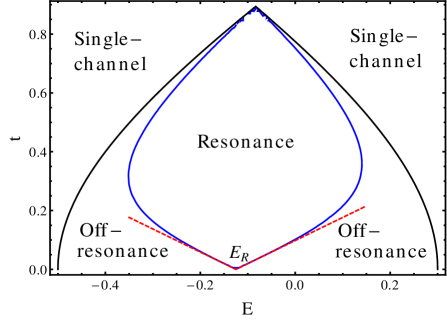
Figure 3: The resonant and off-resonant regimes on the $E-t$ plane for $t_{1}=1$, $t_{2}=0.2$, with isotropic disorder $\sigma_{1}^{2}=\sigma_{2}^{2}$ and bias $\delta{e}=-0.1$. The black curve indicates the band edges $E=E_{1}^{-}$ and $E=E_{2}^{+}$, beyond which only one channel exists. The blue curve marks the crossover line $\Delta{V}=0$. At small enough $t$, $\Delta{V}=0$ can be linearized to $t\simeq\kappa|E-E_{R}|$, cf. Eq. (85), which is plotted as the red dashed line.

In Eq. (80), $\text{w}_{2}(u)$ is simply the analytical continuation of $\text{w}_{1}(u)$. To show this, we start form $\Delta{V}>0$ side and drop the absolute value on $\Delta{V}$. If $\Delta{V}$ crosses zero from above, namely $\Delta{V}\rightarrow-\Delta{V}$, $q_{1}$ changes continuously to $-q_{1}$, and $q_{2}$ changes to one of the two branches $\pm{i}|{q_{2}}|$ because of the square root. It can be easily verified that

$$\text{w}_{1}(u;-q_{1},\pm{i}|q_{2}|)=\text{w}_{2}(u;q_{1},|q_{2}|),$$ (84)

by the formula $\arctan{z}=i/2\ln[(1-iz)/(1+iz)]$ for a complex number $z$.

Given the physical meaning of the parameter $u$, it is natural to interpret the analytical continuation as describing the crossover between two regimes of the polarization, as controlled by the relative strength of the effective disorders. If $\Delta V>0$ (i.e., $V_{1}+V_{2}>4V_{3}$) the intra-channel scattering is stronger than the inter-channel scattering, while $\Delta V<0$ means the opposite. The two regimes can be distinguished quantitatively. According to Eq. (60), the co-efficients in the linear combination of the effective disorder parameters, $\chi^{2}_{\nu}$, are determined by the bare “mixing angle” $\gamma$ and the rapidities, $v_{\tau}$. Suppose the resonance energy $E_{R}$ is approached while keeping $t<t_{c}$ [see Eq. (17)]. If $E$ is in the vicinity of $E_{R}$, $\gamma\sim\pi/2$, and $\Delta{V}<0$. Otherwise, if $E$ is far enough from $E_{R}$, $\gamma\rightarrow 0$ or $\pi$, and $\Delta{V}>0$. Therefore, there must be an energy interval around $E_{R}$, in which the physics is similar to that at resonance, $\gamma=\pi/2$. Further away from $E_{R}$ the physics is similar to the limiting cases $\gamma=0$ or $\pi$. We call $\Delta{V}<0$ and $\Delta{V}>0$ the resonant and off-resonant regimes, whose distinct behavior we will analyze below.

IV.1 Resonant and off-resonant regimes

As shown in Fig. 3, for fixed $t_{\nu}$ and $\delta{e}$, $\Delta V=0$ (blue curve) divides the $E-t$ plane into two regions in the two-channel regime (below the black curve). Three important observations are in order:

(i) At weak coupling $t$, more precisely, for $t\ll t_{c}$, but still within the condition (62), the relation $\Delta V=0$ for the border of the resonance region implies the linear relation (see the red dashed lines in Fig. 3)

$$t\simeq\kappa(t_{1},t_{2})|E-E_{R}|,$$ (85)

with

$$\kappa(t_{1},t_{2})=\frac{t_{1}-t_{2}}{\sqrt{t_{1}^{2}+t_{2}^{2}}}.$$ (86)

The slope $\kappa(t_{1},t_{2})$ neither depend on $\sigma^{2}_{\nu}$ nor on $\delta{e}$.

(ii) If the coupling $t$ is strong enough, the resonance energy interval shrinks to zero as $t\rightarrow t_{c}$ (the top edge of Fig. 3). This “re-entrance” behavior is due to the competition between the strong coupling, which pulls $\gamma$ close to $\pi/2$, and the band edge effect, which reduces the rapidity of one of the channels. We can illustrate this behavior by considering two limiting cases. If $t$ is weak, its effect is of first order on $\gamma$, but of second order on the $v_{\tau}$. Therefore, the coupling wins and the resonance energy interval follows the linear relation (85). Alternatively, if the energy is in the vicinity of the band edges $E=E_{1}^{-}$ and $E_{2}^{+}$, one of the rapidities tends to zero. As a consequence, $V_{1}$ or $V_{2}$ is much larger than $V_{3}$, which gives a large positive $\Delta{V}$. Therefore, there is always some region around the band edges (black curves in Fig. 3), which is out of resonance. As the crossover line must match the two limits $t\to 0$ and $t\to t_{c}$, it is necessarily re-entrant.

(iii) In the case of a non-zero detuning energy $\delta{e}$ the resonant energy interval is slightly asymmetric around $E=E_{R}$.

IV.2 Fixed point distribution $\text{w}(u=\cos\theta)$

Let us now discuss the distribution Eq. (80) in different regimes and some of its consequences. For this purpose, we plot in Fig. 4 some representative $\text{w}(u)$ together with the expectation value and variance of $u$. We select various values of $E$ across the resonant and off-resonant regime. Two types of behavior can be observed in the two regimes:

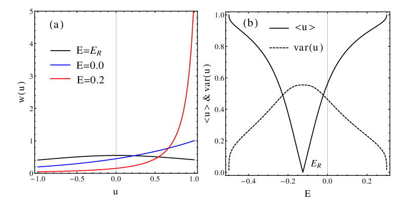
Figure 4: Marginal probability distribution for the angular variable $u=\cos(\theta)$, $\text{w}(u)$, in different regimes. Here the inter-chain coupling $t=0.1$ and the other parameters are the same as in Fig. 3. (a) Distributions $\text{w}(u)$ for three energies across the resonance and off-resonance regimes, namely, $E=E_{R}\approx-0.13$ (i.e., resonance energy), $E=0.2$ (off-resonance) and $E=0.0$ (crossover). On resonance the distribution is nearly uniform, while it is strongly non-uniform off-resonance (b) The expectation value and variance of $u$ as functions of $E$.

(i) Near the resonance, $u=\cos\theta$ is distributed relatively uniformly in the interval $(-1,1]$. Its average value is much smaller than 1, but its variance is large of order $O(1)$. However, the distribution is definitely not completely uniform. Indeed, the limit of the distribution can be obtained form Eq. (80) in the weak coupling limit as $t\rightarrow 0$ as

$$\text{w}(u)=\frac{3\sqrt{3}}{\pi(3+u^{2})},$$ (87)

which is manifestly non-uniform. A similar distribution was obtained by Dorokhov dorok in the case of two equivalent chains. We will discuss the difference to Eq. (87) later.

(ii) Off resonance, the distribution function $\text{w}(u)$ is strongly peaked at $u=1$, and its fluctuations are strongly suppressed.

At this point the difference between the canonical DMPK equation,dorok ; mpk1 ; mpk2 which applies in the case $N\gg 1$, and the extended DMPK equation obtained here for the case $N=2$, is clear. The isotropy assumption, which allows one to derive the canonical DMPK equation, states that the angular variable distribution $\text{w}(u)$ should be uniform, i.e., independent of $u$, in contrast to Eq. (87). In order to justify the canonical DMPK equation, we have to have a large number of equal chains. A sufficient condition for obtaining the canonical DMPK equation is that the probability distribution of the transfer matrices of an “elementary slice” is invariant under $U(N)$ rotation. This situation may be achieved in thick wires.mpk1 ; mpk2 However, in few-channel cases the localization lengths are larger, but still of the same order as the mean free path. There is no parametric window between them that permits the emergence of $U(N)$-invariant ensembles of transfer matrices upon coarsegraining.

The qualitative difference in the distribution function $\text{w}(u)$ in the two regimes has important implications on the localization lengths. To calculate the localization lengths from Eq. (75), we need $\langle\Gamma_{6}\rangle$ and $\langle u\rangle$. Using Eq. (80) we obtain

$$\langle\Gamma_{6}\rangle=\begin{cases}\frac{q_{1}q_{2}|\Delta{V}|S_{1}(q_{1},q_{2})}{2\sinh{\left(\frac{q_{1}}{q_{2}}\arctan{\frac{1}{q_{2}}}\right)}}-4V_{3}&\Delta{V}\leq 0,\\ &\\ \frac{q_{1}q_{2}|\Delta{V}|\tilde{S}_{1}(q_{1},q_{2})}{2\sinh{\left(\frac{q_{1}}{2q_{2}}\ln{\frac{q_{2}+1}{q_{2}-1}}\right)}}-4V_{3}&\Delta{V}\geq 0,\end{cases}$$ (88)

and

$$\langle u\rangle=\begin{cases}\frac{q_{1}S_{2}(q_{1},q_{2})}{2\sinh{\left(\frac{q_{1}}{q_{2}}\arctan{\frac{1}{q_{2}}}\right)}}&\Delta{V}\leq 0,\\ &\\ \frac{q_{1}\tilde{S}_{2}(q_{1},q_{2})}{2\sinh{\left(\frac{q_{1}}{2q_{2}}\ln{\frac{q_{2}+1}{q_{2}-1}}\right)}}&\Delta{V}\geq 0,\end{cases}$$ (89)

where $S_{1(2)}$ and $\tilde{S}_{1(2)}$ are integrals defined by

$$\begin{split}S_{1}(q_{1},q_{2})&=\int_{-\arctan{(1/q_{2})}}^{\arctan{(1/q_{2})}}{dz\sec^{2}{z}\,e^{\frac{q_{1}}{q_{2}}z}},\\ S_{2}(q_{1},q_{2})&=\int_{-\arctan{(1/q_{2})}}^{\arctan{(1/q_{2})}}{dz\tan{z}\,e^{\frac{q_{1}}{q_{2}}z}},\\ \tilde{S}_{1}(q_{1},q_{2})&=\int_{-1/q_{2}}^{1/q_{2}}{dz\left(\frac{1+z}{1-z}\right)^{\frac{q_{1}}{2q_{2}}}},\\ \tilde{S}_{2}(q_{1},q_{2})&=\int_{-1/q_{2}}^{1/q_{2}}{dz\frac{z}{1-z^{2}}\left(\frac{1+z}{1-z}\right)^{\frac{q_{1}}{2q_{2}}}}.\end{split}$$ (90)

IV.3 Numerical analysis

In order to confirm our analytical results for the localization lengths in Eq. (75) we calculated numerically the Lyapunov exponents of the products of transfer matrices in Eq. (30). An efficient numerical method, known as the reorthogonalization method, has been developed in the study of dynamical systemsbggs-cpv and widely spread in the field of Anderson localization.mac-kram The forthcoming numerical results in Figs. 5-8, 10 and 11 are all obtained by this method.

The usefulness of the reorthogonalization method is not restricted to numerical simulations. It also provides the basis for the perturbative analysis about the Lyapunov exponents in the weak disorder limit in Sec. VI.2.

V Results for the localization lengths

In order to reveal the effects of the transverse coupling $t$ on the localization lengths, we define the two ratios

$$r_{\rho}=\xi_{\rho}/\xi_{\rho}^{(0)},\quad\rho\in\{1,2\},$$ (91)

where the $\xi_{\rho}^{(0)}$s are the localization lengths of the decoupled legs, for which we may assume $\xi_{1}^{(0)}\geq\xi_{2}^{(0)}$. For simplicity, we refer to the leg $1$ and $2$ as the fast- and the slow-leg, respectively. The bare localization lengths $\xi_{\rho}^{(0)}$ can easily be obtained from Eq. (75) by taking $\gamma=0$, $\text{w}(u)=\delta(u-1)$ and $t=0$, which yields

$$\xi_{\rho}^{(0)}=\frac{2v_{\rho}^{2}}{\chi^{2}_{\rho}}.$$ (92)

Eq. (92) coincides with the well-known single-chain result.mel

V.1 $E=0$ and $\delta{e}=0$: Resonant regime

Consider first the case $\delta{e}=0$, in which the resonance energy vanishes $E_{R}=0$. From Eqs. (12) and (18) it follows that the mixing angle is $\gamma=\pi/2$ once $t\neq 0$, and the two rapidities $v_{1}=v_{2}=v$ are equal to each other:

$$v^{2}=4-\frac{t^{2}}{t_{1}t_{2}}.$$ (93)

Consequently, the three Born cross-sections have the same value and are equal to:

$$V_{1}=V_{2}=V_{3}=V=\frac{1}{16v^{2}}{\left(\chi^{2}_{1}+\chi^{2}_{2}\right)}.$$ (94)

This gives $q_{1}=0$ and $q_{2}=\sqrt{3}$ according to Eqs. (81) and (83). Evaluating the integrals (90), we obtain the two localization lengths

$$\xi_{\rho}=8C_{\rho}v^{2}/{\left(\chi^{2}_{1}+\chi^{2}_{2}\right)},$$ (95)

where

$$C_{1}=\frac{\pi}{3(\pi-\sqrt{3})}\approx 0.743,$$ (96a)

and

$$C_{2}=\frac{\pi}{\pi+3\sqrt{3}}\approx 0.377.$$ (96b)

The corresponding decoupled values ($t=0$) can easily be obtained from Eq. (92),

$$\xi_{\rho}^{(0)}=\frac{8}{\chi^{2}_{\rho}}.$$ (97)

Therefore, the ratios defined by Eq. (91) read

$$r_{\rho}=C_{\rho}v^{2}\chi^{2}_{\rho}/{\left(\chi^{2}_{1}+\chi^{2}_{2}\right)}.$$ (98)

Notice that in the resonant case, the Born cross-sections (60) are dominated by $\chi^{2}_{2}$, which gives rise to the dramatic drop of the localization length of the fast leg: The slow-leg is dominating the backscattering rate and thus the localization length.

From Eq. (98) we draw several important conclusions below.

V.1.1 Statistically identical chains

For two coupled chains, which are statistically identical, one has $\chi^{2}_{1}=\chi^{2}_{2}$, and we obtain

$$\frac{\xi_{1}}{\xi_{1}^{(0)}}\equiv r_{1}=2C_{1}\approx 1.486,$$

$$\frac{\xi_{2}}{\xi_{2}^{(0)}}\equiv r_{2}=2C_{2}\approx 0.754.$$ (99)

We note that $r_{1}$ is slightly larger than the value obtained by Dorokhovdorok , which is $\pi/(\pi-1)\approx 1.467$. The reason is that we have taken into account the forward-scattering in the “elementary slice” (27), which was neglected in the work by Dorokhov. Moreover the latter was restricted to $t_{1}=t_{2}$. In Fig. 5 we compare our analytical prediction with Dorokhov’s. Note that we take $E=0.1$ in the numerical simulation in order to avoid the anomaly at $E=0$, as mentioned in Sec. III.4. The enhancement factor $r_{1}$ is essentially independent of the selected energy if $t$ is weak enough. This is due to the fact that any energy is at resonance conditions for $t_{1}=t_{2}$.

The effect of forward scattering, which was included in our work, is clearly visible. It is confirmed by the numerical simulation at resonance conditions. However, the value $r_{1}\approx 1.776$ obtained by Kasner and Wellerkas-wel deviates significantly from our numerical and analytical results.

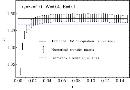
Figure 5: Ratio of coupled and uncoupled localization lengths, $r_{1}=\xi_{1}/\xi_{1}^{(0)}$, for statistically identical chains with $t_{1}=t_{2}=1$ and small disorder $W$. We consider small couplings $t$, for which any energy is at resonance conditions. In the numerical simulation we take $E=0.1$ in order to avoid the anomaly at $E=0.0$. However, according to Eq. (V.1.1), $r_{1}$ is almost independent of $E$ if $t$ is weak enough. The continuum approximation becomes exact for $W^{2}\ll t\ll 1$, as is illustrated by the convergence of the numerical data to the analytical prediction (the agreement is already good for $cW^{2}\lesssim t$ with $c\approx 0.25$). For comparison we also plot Dorokhov’s prediction dorok , which neglected forward scattering in the Fokker-Planck equation. The result of Kasner and Wellerkas-wel ($r_{1}\approx 1.776$) is in clear contradiction with these numerics.

V.1.2 Parametrically different chains

It is interesting to analyze what happens if the bare localization lengths of the chains are parametrically different $\xi^{(0)}_{2}\ll\xi^{(0)}_{1}$. In the resonant regime, for $W^{2},|E-E_{R}|\ll t\ll t_{1},t_{2}$, we obtain:

$$\xi_{1}\rightarrow 4C_{1}\,\xi^{(0)}_{2}\approx 2.972\,\xi^{(0)}_{2},$$ (100a)

$$\xi_{2}\rightarrow 4C_{2}\,\xi^{(0)}_{2}\approx 1.507\,\xi^{(0)}_{2}.$$ (100b)

Eq. (100) is one of the central results in this paper: In the resonant regime, the localization length of the fast leg is dramatically dragged down by the slow-leg. In contrast, the localization length of the slow leg is increased by the presence of the fast leg, but remains of the same order. As a result both localization lengths become of the order of that for the bare slow leg. This is illustrated for two different cases of coupled fast and slow legs in Figs. 6 and 7. Fig. 6 shows the effect in the case of legs with equal disorder but different hopping strength, the resonance being at $E=0$. In Fig. 7 the faster leg has the same hopping but weaker disorder. Here the legs are resonant at every energy below the band-edge $E_{2}^{+}$.

We note that there is no regime where both $r_{1}>1$ and $r_{2}>1$, as this would contradict the equality $\sum_{\rho}{r_{\rho}/C_{\rho}}=v^{2}$, which follows from Eq. (98). At the band center and $t\to 0$ one can achieve that both localization lengths do not decrease upon coupling the chains, $r_{1}=r_{2}=1$. This happens when $\chi^{2}_{2}/\chi^{2}_{1}=4C_{1}-1$, which assures that the localization lengths do not change at coupling constants $t\lesssim W^{2}$ according to the discussion in Sec. V.1.3.

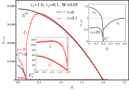
Figure 6: Localization lengths for chains with different hopping strengths ($t_{1}=1$ and $t_{2}=0.1$), but equal disorder ($W=0.05$) as a function of energy at detuning $\delta{e}=0$ and intermediate coupling $t=0.1$. The solid curves are analytical results. Black curves correspond to uncoupled chains, red ones to the coupled chains. The squares and circles are data of the numerical transfer matrix. $\xi_{2}^{(0)}$ and $\xi_{2}$ are amplified 20 times to increase visibility, but $\xi_{1}>\xi_{2}$ always holds. The lower left insert is a zoom in the two-channel region. The upper right insert shows the ratios $r_{1,2}$ of coupled to uncoupled localization lengths. The larger localization length is very significantly suppressed due to the coupling to a slow chain. Note the sharp recovery of the larger localization length beyond the band-edge $E_{2}^{+}$. The analytical results coincide quantitatively with the numerical data anywhere except for specific anomalous energies: In the uncoupled case, $E=0$ corresponds to the commensurate wave vectors $4k_{1(2)}=2\pi$. In the coupled case, $E=0$ and $E\approx 0.03$, $0.1$ (very weak) and $0.17$ correspond to $2(k_{1}+k_{2})=2\pi$, $3k_{1}+k_{2}=2\pi$, $4k_{1}=2\pi$ and $3k_{2}-k_{1}=2\pi$.

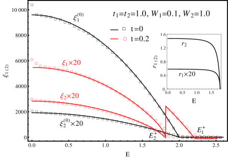
Figure 7: Localization lengths for the decoupled ($t=0$, black) and coupled ($t=0.2$, red) chains with identical hopping but substantially different disorder ($W_{1}=0.1$ and $W_{2}=1.0$) as a function of energy (detuning $\delta{e}=0$). The solid curves are analytical results. The squares and circles are data from the numerical transfer matrix. The values of $\xi_{1}$, $\xi_{2}^{(0)}$ and $\xi_{2}$ are amplified 20 times to increase their visibility. Without coupling $\xi_{1}^{(0)}/\xi_{2}^{(0)}\sim 10^{2}$. In the presence of coupling $\xi_{1}$ is substantially reduced, while $\xi_{2}$ remains of the same order as its decoupled value. The insert shows the ratios $r_{1,2}$ of coupled to uncoupled localization lengths. Since $t_{1}=t_{2}$ there is resonance at all energies, and thus dominance of the slow chain is expected. Note the sharp recovery of the larger localization length beyond the band-edge $E_{2}^{+}$. There are visible anomalies at $E=0$ in both the uncoupled and the coupled case, which correspond to the commensurate condition $4k_{1(2)}=2\pi$ and $2(k_{1}+k_{2})=2\pi$. In the coupled case further anomalies exist at the energies corresponding to $3k_{1}+k_{2}=2\pi$, $4k_{1}=2\pi$ and $3k_{2}-k_{1}=2\pi$. However, they are every close to $E=0$ and too weak to be observed.

V.1.3 Weak coupling limit

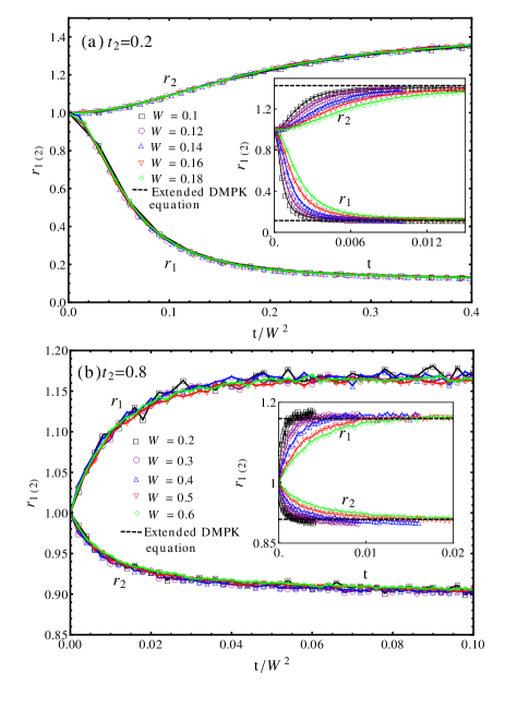
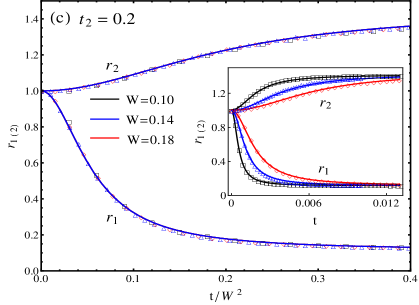
Figure 8: The ratio $r_{1,2}=\xi_{1,2}/\xi^{(0)}_{1,2}$ of coupled and decoupled localization lengths, obtained numerically as a function of the coupling constant $t$ at resonant conditions, $E=0$ and $\delta{e}=0$. The two legs are equally disordered with a random potential box distributed in $[-W/2,W/2]$. (a) A slow $t_{2}=0.2$ and a fast $t_{1}=1$ leg: The smaller localization length increases slightly while the larger localization length decreases drastically, being driven down by the slow leg, as the coupling constant $t$ increases. The insert shows the dependence of $r_{1,2}$ on the coupling constant $t$ at different disorder strengths; all the curves collapse to a universal dependence on $t/W^{2}$. The dashed lines in the insert show the analytic result given by Eq. (98), which is valid under the assumption $t\gg W^{2}$, Eq. (62). (b) Almost identical legs $t_{2}=0.8$, $t_{1}=1$: In this case the localization length of the slow leg marginally decreases while that of the fast leg marginally increases. (c) Results obtained analytically upon replacing the mixing angle with a renormalized value, $\gamma\to\tilde{\gamma}$. The parameters are the same as in (a) but with fewer realizations of disorder, and $\delta E/W^{2}\approx 0.3$ in Eq. (103) was optimized by fitting to the numerical data in (a). The scaling collapse works very well in the weak coupling limit.

Upon simply taking the $t=0$ limit,

$$r_{\rho}=4C_{\rho}\chi^{2}_{\rho}/{\left(\chi^{2}_{1}+\chi^{2}_{2}\right)},$$ (101)

one does not recover the decoupled values $r_{\rho}=1$. This should indeed be expected, as we have already discussed in Sec. III.3. The reason traces back to condition (62) to obtain Eq. (68), namely that $t$ be larger than the disorder energy scale $\delta{E}\propto W^{2}$. In order to verify the non-commutativity of $t\to 0$ and $W\to 0$, we computed numerically the localization lengths by the transfer matrix approach, and obtained the values of $r_{\rho}$ down to very small values of $t$, cf. Fig. 8). In this simulation, the re-orthogonalization method mac-kram was used, and length of the ladder is $L=10^{7}$ with averaging over $10^{3}$ realizations of disorder. The hopping integral in the fast chain $t_{1}=1$ was taken as the energy unit, and for simplicity, the two legs were taken to be equally disordered. One can see that as the coupling $t$ increases the quantities $r_{1,2}$ evolve and at $t\gg W^{2}$ approach the limits given by Eq. (101).

The insensitivity of the localization lengths to weak couplings $t\ll\delta E$ reflects the fact that the level spacing in the chains is bigger than the coupling between the chains, and thus wavefunctions typically do not hybridize much between the two legs.

Moreover, the two families of curves for different disorder strengths seem to collapse into two universal functions $r_{1,2}(t/W^{2})$, c.f. Fig. 8. This scaling shows that at weak disorder $W\ll 1$ and under resonance conditions $E=E_{R}$, the numerical results approach the analytical ones already at a very small coupling $t\gtrsim W^{2}$.

We can rationalize the scaling by defining a regularized mixing angle $\tilde{\gamma}$ instead of the bare $\gamma$ defined by Eq. (12). From Eqs. (12) and (85), we find that

$$\tan^{2}{\gamma}\propto\frac{t^{2}}{[\kappa(t_{1},t_{2})(E-E_{R})]^{2}}.$$ (102)

where $\kappa(t_{1},t_{2})$ is defined in Eq. (86). A natural way of regularizing the above result at resonance conditions is to introduce the disorder-induced “width” $\delta E\propto W^{2}$ in the form:

$$\tan^{2}{\tilde{\gamma}}\propto\frac{t^{2}}{[\kappa(t_{1},t_{2})(E-E_{R})]^{2}+\delta{E}^{2}},$$ (103)

where $\delta{E}$ scales as in Eq. (63).

Using this regularized mixing angle, the resonant regime can be described more precisely by the condition

$$t\gg\max\{\kappa(t_{1},t_{2})|E-E_{R}|,\delta{E}\},$$ (104)

or, equivalently, $\tilde{\gamma}\sim\pi/2$. The observed scaling collapse in Fig. 8(a) suggests that in the weak coupling one might capture the behavior of localization lengths by replacing $\gamma$ by $\tilde{\gamma}$ in Eq. (60). This indeed works, as confirmed by Fig. 8(c) where we replot the numerical data of Fig. 8(a) together with the analytical expressions, where $\tilde{\gamma}$ replaces $\gamma$, and the number $\delta E/W^{2}\approx 0.3$ was optimized to yield the best fit.

Note that the resonance condition can be broken either by detuning $|E-E_{R}|\gg t$ or by increasing the disorder $\delta E\gg t$. Our analytic approach is based on the weak-disorder expansion and is therefore valid only in the first regime.

V.1.4 Anomalies

One can notice that all our numerical curves for $\xi_{1,2}$ exhibit anomalies which are not predicted by the analytical curves: small “peaks” appear at certain energies on both $\xi_{1}$ and $\xi_{2}$. These anomalies of localization lengths are due to the commensurability discussed in Sec. III.4. This is not captured by the extended DMPK equation (68). However, we can identify these anomalous energies with commensurate combinations of wave vectors in Eq. (III.4) (see the caption in Figs. 6 and 7). The anomalies for two chains with identical hopping but different disorder have been observed numerically in Ref. ngu-kim, . In this case there are three anomalous energies $E=0$, $t/2$ and $t$, which correspond to commensurate combinations of wave vectors $2(k_{1}+k_{2})=2\pi$, $3k_{1}+k_{2}=2\pi$ and $4k_{1}=2\pi$.

V.2 Solutions at $E\neq 0$: off-resonant regime

Without loss of generality the off-resonant regime can be considered at $\delta e=0$ (for which the resonance is at $E_{R}=0$). A non-zero detuning $\delta{e}$ merely drives $E_{R}$ away from zero and induces an asymmetry of the $r_{\rho}$ as a function of $E-E_{R}$. However, the mechanism of the crossover from resonance to off-resonance is qualitatively the same as in the case $\delta{e}=0$.

Our analytical results for $r_{1,2}$ are presented in Fig. 9 as functions of the dimensionless detuning $E/t$ from resonance.

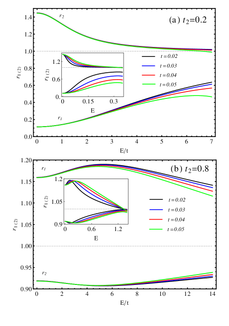
Figure 9: Analytical results for $r_{1,2}=\xi_{1,2}/\xi^{(0)}_{1,2}$ as functions of $E$ and $E/t$ obtained from the extended DMPK equation in the weak disorder case $\delta E\ll t$ for detuning $\delta{e}=0$. The resonance energy corresponds to $E_{R}=0$. (a) $t_{2}=0.2$, $t_{1}=1$. (b) $t_{2}=0.8$, $t_{1}=1$. Close to resonance the $r_{\rho}$ only depend on the ratio $E/t$.

(i) Small detuning, $|E|\ll t/\kappa(t_{1},t_{2})\ll 1$: The resonance conditions are still fulfilled and the localization lengths are close to their corresponding values at $E=0$. The leading order expansion around $\gamma=\pi/2$ predicts that the ratios of localization lengths, $r_{1,2}$ only depend on $E/t$, but not on $t/t_{1}$,

$$\left|r_{\rho}-r_{\rho}(E=0)\right|\propto\left(\frac{E}{t}\right)^{2},$$ (105)

as confirmed numerically in Fig. 9.

(ii) Very large detuning, $|E|\gg t/\kappa(t_{1},t_{2})\gg 1$, $r_{1(2)}$ approaches $1$ from below (above) like

$$\left|r_{\rho}-1\right|\propto t^{2}.$$ (106)

When $t$ is small this result is obtained from the leading order expansion of $r_{\rho}$ around $\gamma=0$ or $\pi$.

(iii) For chains with equal hopping, $t_{1}=t_{2}$, resonance occurs at any energy and $r_{\rho}=2C_{\rho}$ is independent of $E/t$.

V.3 Band-edge behavior

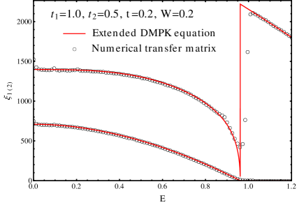
Figure 10: Localization lengths as a function of energy near the edge of one of the bands. Here $W=0.2$, $t_{1}=1$, $t_{2}=0.5$, $t=0.2$ and $\delta{e}=0$. The red curve is the result of the extended DMPK equation, while the black circles are data obtained by the numerical transfer matrix method. The quantitative agreement is significant except for four anomalous energies, e.g. $E=0$ and $E\approx 0.1$, $0.2$ and $0.9$. The correponding commesurate combinations of wave vectors are $2(k_{1}+k_{2})=2\pi$, $3k_{1}+k_{2}=2\pi$, $4k_{1}=2\pi$ and $3k_{2}-k_{1}=2\pi$. Near the termination of the lower band at $E<E_{2}^{+}$ the larger localization length is dramatically decreased, driven down by the slow terminating channel. At $E>E_{2}^{+}$ the localization length sharply recovers. In numerical simulation the sharpness is smeared by the finite disorder.

Another interesting question to ask is what happens to the localization lengths around the band-edge $E_{1}^{-}$ or $E_{2}^{+}$? (See Fig. 1(a)) Especially, what is the behavior of the localization length of the fast-leg once we turn on the coupling $t$? The results from the numerical transfer matrix simulation and of the solution (75) of the extended DMPK equation, Eq. (68), are compared in Fig. 10.

Two remarkable features can be observed in Fig. 10:

(i) Near the band edge $E=E_{2}^{+}$ where the system switches from one to two propagating channels, the larger localization length $\xi_{1}$ (red curves) behaves in a singular way, as obtained from Eq. (75). As the energy tends to the band-edge $E_{2}^{+}$ from below, $\xi_{1}$ decreases to zero and shows a jump to a finite value for $E>E_{2}^{+}$, where only one propagating channel exists. The numerical simulation (black circles) reproduces the same behavior, while the sharp recovering at $E=E_{2}^{+}$ is smeared by the finite disorder. This behavior is another drastic example of the dominant effect of the slow channel. It can be understood from the behavior of the Born cross-sections Eq. (60). As we approach the band-edge from below, the rapidities of the two channels satisfy $v_{1}\gg v_{2}$. As a consequence, the cross-sections obey the hierarchy $V_{2}\gg V_{3}\gg V_{1}$. Therefore, from Eq. (80) and (75), one can see that $\xi_{1}$ is dominated by the largest cross section $V_{2}$ and shows qualitatively the same behavior as $\xi_{2}$. We emphasize that the mechanism of this suppression is different from that in the resonant regime. In the latter the suppression is due to $\gamma\sim\pi/2$, which mixes the two effective variances $\chi^{2}_{\nu}$ equally, while near the band-edge the suppression is due to the vanishing rapidity, which appears in the denominators of the cross-sections.

(ii) Anomlies are clearly seen in the numerical data for $\xi_{1}$ at energies $E=0$ and $E\approx 0.1$, $0.2$ and $0.9$. The corresponding commensurate combinations of wave vectors are $2(k_{1}+k_{2})=2\pi$, $3k_{1}+k_{2}=2\pi$, $4k_{1}=2\pi$ and $3k_{2}-k_{1}=2\pi$.

VI one-channel regime

So far we have discussed the localization lengths in the two-channel regime, where the extended DMPK equation (68) applies. In the one-channel regime (see Fig. 1) the second channel does not vanish but supports evanescent modes. In the presence of disorder a particle in propagating modes can be scattered elastically into these evanescent modes by local impurities. Thus the evanescent channel is coupled to the propagating channel by random potentials and may influence the transport properties of the system. However, the effect of evanescent modes in the transport properties of 1D disordered systems is scarcely studied.

Bagwellbag studied in detail the transmission and reflection coefficients in a multi-channel wire with a single $\delta$-function impurity. The evanescent modes renormalize the matrix elements of the impurity potential in the propagating channels. The transmission and reflection coefficients of the propagating channels can be strongly enhanced or suppressed, nevertheless, depending on the strength of the impurity.

The model in Ref. bag, was non-disordered but quite relevant to disordered systems. It is reasonable to argue that in 1D disordered systems the effective disorder in the propagating channels is renormalized by evanescent modes, while the renormalization effect depends upon the strength of disorder.

In the present two-leg Anderson model we specifically analyze the renormalization effect of the evanescent channel in the weak disorder limit, which stands on an equal footing with the analysis in the two-channel case. Actually, the special case $t_{1}=t_{2}$ and $\sigma_{1}^{2}=\sigma_{2}^{2}$ has been studied analytically early on in Ref. heinrich, . It was claimed that in the weak disorder limit the effective disorder in the propagating channel is significantly suppressed by the evanescent mode. As a consequence, the localization length defined through the transmission coefficient of the propagating channel is enhanced by a factor $\sim 2$ compared to the value obtained if the evanescent mode is absent. However, this conclusion was unreliable because the average of the logarithm of transmission eigenvalue was not computed correctly. In contrast, we will prove that the evanescent channel is decoupled from the propagating channel to the lowest order in the effective disorder $\chi_{\nu}^{2}$ defined in Eq. (48). The coupling between the two channels becomes relevant only at order $\chi_{\nu}^{4}$.

VI.1 Transfer matrix of an elementary slice

Without loss of generality, we assume that the channel $\tau=1$ is propagating and $\tau=2$ is evanescent (the upper branch in Fig. 1). A similar analysis applies to the opposite choice (the lower branch in Fig. 1). Note first of all that a direct application of the Fokker-Planck equation approach to the transfer matrix given in Eqs. (27) and (30) would be incorrect. The reason is the following: The weak disorder expansion of the parameters $\vec{\lambda}$, which leads to Eq. (51), is ill-defined in the one-channel regime. Note that the amplitude of the evanescent basis $\psi_{2}(x)$ (see Eq. (26)) grows exponentially $\sim e^{\kappa_{2}|x|}$. Likewise, the elements of $\delta{\mathbf{m}}_{x}$ (see Eq. (27)) with evanescent channel indices also grow exponentially with factors $e^{2\kappa_{2}|x|}$ or $e^{4\kappa_{2}|x|}$. Therefore, $\|\delta{\mathbf{m}}_{x}/{\epsilon}\|$ is unbounded in the domain of the coordinate $x$, and the formal expansion of the parameters $\vec{\lambda}$ in disorder strength is divergent with respect to the length $L$.eva-div

In order to perform a weak disorder analysis, the basis of the evanescent channel should be chosen as

$$\psi_{2}^{\pm}(x)=e^{\mp\kappa_{2}x}/\sqrt{2\sinh{\kappa_{2}}},\quad\kappa_{2}>0,$$ (107)

which replaces the current-conserving basis Eq. (26), and the basis of the propagating channel is the same as Eq. (24) even though with $\tau=1$. In this newly defined basis, the transfer matrix of elementary slice takes the form: (see App. D)

$$\mathbf{m}_{x}=\mathbf{m}+\delta{\mathbf{m}}_{x},$$ (108)

with

$$\mathbf{m}=\text{diag}\left(1,\,\,1,\,e^{-\kappa_{2}},\,e^{\kappa_{2}}\right),\quad\delta{\mathbf{m}}_{x}=\begin{pmatrix}\delta m_{1}^{1}&\delta m_{2}^{1}\\ \delta m_{1}^{2}&\delta m_{2}^{2}\end{pmatrix},$$ (109)

whose blocks are

$$\delta m_{1}^{1}=i\frac{{\epsilon}_{\text{11}}}{2\sin{k_{1}}}\begin{pmatrix}-1&-e^{-i2k_{1}x}\\ e^{i2k_{1}x}&1\end{pmatrix},$$ (110a)

$$\begin{split}\delta m_{2}^{1}=&i\frac{{\epsilon}_{\text{12}}}{2\sqrt{\sin{k_{1}}\sinh{\kappa_{2}}}}\\ &\times\begin{pmatrix}-e^{-\kappa_{2}}e^{-ik_{1}x}&-e^{\kappa_{2}}e^{-ik_{1}x}\\ e^{-\kappa_{2}}e^{ik_{1}x}&e^{\kappa_{2}}e^{ik_{1}x}\end{pmatrix},\end{split}$$ (110b)

$$\delta m_{1}^{2}=\frac{{\epsilon}_{\text{21}}}{2\sqrt{\sin{k_{1}}\sinh{\kappa_{2}}}}\begin{pmatrix}-e^{ik_{1}x}&-e^{-ik_{1}x}\\ e^{ik_{1}x}&e^{-ik_{1}x}\end{pmatrix},$$ (110c)

$$\delta m_{2}^{2}=\frac{{\epsilon}_{\text{22}}}{2\sinh{\kappa_{2}}}\begin{pmatrix}-e^{-\kappa_{2}}&-e^{\kappa_{2}}\\ e^{-\kappa_{2}}&e^{\kappa_{2}}\end{pmatrix},$$ (110d)

where $\mathbf{m}$ and $\delta{\mathbf{m}}_{x}$ are the disorder-free and disordered part of the elementary slice $\mathbf{m}_{x}$. The transfer matrix of a bulk with length $L$ is still defined by the products in Eq. (30). Two important points should be emphasized:

(i) Compared with Eq. (27) in the two-channel case, the second and third rows and columns of Eq. (108) have been simultaneously permuted. The diagonal blocks $\delta m_{1}^{1}$ and $\delta m_{2}^{2}$ represent the scattering in the propagating and evanescent channel, respectively, and the off-diagonal blocks $\delta m_{2(1)}^{1(2)}$ represent the scattering between the two channels. In each block, the first and second diagonal element describe the scattering inside right- ($+$) and left- ($-$) branch respectively, and the off-diagonal elements describe the scattering between the two branches. For instance, $\delta m_{1+}^{2-}$ labels the $21$-element of $\delta m_{1}^{2}$ and stands for a scattering event from the left evanescent channel to the right propagating channel.

(ii) The disordered part $\delta{\mathbf{m}}_{x}$ does not contain exponentially growing and/or decaying terms, and hence $\|\delta{\mathbf{m}}_{x}/{\epsilon}\|$ is uniformly bounded for any $x$. Instead, the disorder-free part $\mathbf{m}$, which is still diagonal but not unity any more, contains the growing and decaying factor of the evanescent mode per lattice spacing. The exponentially growing and decaying characteristics of evanescent modes are represented in the products of the disorder-free part $\prod_{x=1}^{L}\mathbf{m}$.

VI.2 Weak disorder analysis of Lyapunov exponents

In order to calculate the transmission coefficient of the propagating channel, through which the localization length is defined (see Sec. VI.3), we have to know the Lyapunov exponents of $\mathbf{M}(L)$ in Eq. (30). We are going to determine the Lyapunov exponents by the method introduced in Ref. bggs-cpv, .

The Lyapunov exponents of the present model can be computed via the following recursive relations for the four vectors $V_{i=1,\cdots,4}$:

$$V_{1,x+1}=\mathbf{m}_{x}V_{1,x},$$ (111a)

$$V_{i,x+1}=\mathbf{m}_{x}V_{i,x}-\sum_{j=1}^{i-1} {\frac{V_{j,x+1}\cdot\left(\mathbf{m}_{x}V_{i,x}\right)}{V_{j,x+1}\cdot V_{j,x+1}}V_{j,x+1}},$$ (111b)

$$\hskip 28.45274pt2\leq i\leq 4.$$

Note that the vectors are orthogonalized by Gram-Schmidt procedure after every multiplication by the transfer matrices (108). The Lyapunov exponents are extracted form the growing rate of the amplitudes of the respective vectors:

$$\gamma_{i}=\lim_{L\to\infty}\frac{1}{2L}\left\langle\ln{\frac{\left|V_{i,L}\right|^{2}}{\left|V_{i,1}\right|^{2}}}\right\rangle,\quad 1\leq i\leq 4,$$ (112)

in which $\langle\cdot\rangle$ is the average over realizations of disorder along the strip. Moreover, $\{\gamma_{i}\}$ are in descendant order:

$$\gamma_{1}\geq\gamma_{2}\geq\gamma_{3}\geq\gamma_{4}.$$ (113)

The initial vectors $V_{i,1}$ of the recursive relations (111) can be randomly chosen but must be linearly independent. In the absence of specific symmetry constraints the Lyapunov exponents are non-degenerate in the presence of disordered part of $\mathbf{m}_{x}$. Additionally, because of the symplecticity of $\tilde{\mathbf{m}}_{x}$ represented in Eq. (21) the Lyapunov exponents are related by

$$\gamma_{3}=-\gamma_{2},\quad\gamma_{4}=-\gamma_{1},$$ (114)

which is proved in App. D. Therefore, only the first two recursions in Eq. (111) are needed.

In the absence of disorder the four Lyapunov exponents take the values:

$$\gamma_{1}|_{{\epsilon}=0}=\kappa_{2},\quad\gamma_{2}|_{{\epsilon}=0}=\gamma_{3}|_{{\epsilon}=0}=0,\quad\gamma_{4}|_{{\epsilon}=0}=-\kappa_{2},$$ (115)

in which the two Lyapunov exponents corresponding to the propagating channel are degenerate. Therefore, we make an ansatz on the first two vectors, which separates their “moduli” and “directions”,

$$V_{1,x}=v_{1,x}\begin{pmatrix}s_{1}(x)\\ s_{2}(x)\\ s_{3}(x)\\ 1\end{pmatrix},\quad V_{2,x}=v_{2,x}\begin{pmatrix}p(x)\\ q(x)\\ t_{3}(x)\\ t_{4}(x)\end{pmatrix},$$ (116)

in which

$$s_{1,2,3}(x),t_{3,4}(x)\sim O({\epsilon}),$$ (117)

$|s_{1,2,3}(x)/{\epsilon}|$ and $|t_{3,4}(x)/{\epsilon}|$ are bounded for all $x$, and

$$|p(x)|^{2}+|q(x)|^{2}=1.$$ (118)

Eventually, the Lyapunov exponents are determined by the growth rate of $\{v_{i,x}\}$, which is easy to be realized from Eqs. (112) and (116). The initial vectors of Eq. (116) are chosen as the eigenvectors of the disorder-free part of the transfer matrix $\mathbf{m}$ (see Eq. (109)):

$$V_{1,1}=\begin{pmatrix}0\\ 0\\ 0\\ 1\end{pmatrix},\quad V_{2,1}=\begin{pmatrix}p(1)\\ q(1)\\ 0\\ 0\end{pmatrix},$$ (119)

with some $p(1)$ and $q(1)$ satisfying $|p(1)|^{2}+|q(1)|^{2}=1$.

Note that the ansatz (116) is reasonable in the sense of a perturbative analysis. Consider the final vectors after $L$ iterations of Eq. (111) with the initial condition Eq. (119). In the absence of disorder, it is easy to obtain $V_{1,L}=e^{\kappa_{2}L}V_{1,1}$ and $V_{2,L}=V_{2,1}$. On top of it weak enough disorder will induce perturbative effects: the direction of $V_{1,L}$ will deviate from $V_{1,1}$ perturbatively in the strength of disorder. This is characterized by the smallness of $s_{1,2,3}(L)$. In other words, the exponential growth of $|V_{1,L}|$ is dominated by $\mathbf{m}$. Simultaneously, the degeneracy of the second and third exponents are lifted perturbatively. As a consequence, $\gamma_{2}>0$ and $v_{2,L}$ become exponentially large because of the constraint in Eq. (114). $p(L)$ and $q(L)$ are in general very different from their initial values $p(1)$ and $q(1)$, while $t_{3,4}(L)$ will be shown to remain small quantities of order ${\epsilon}$.

The orthogonality between $V_{i,x}$ in Eq. (116) gives

$$t_{4}(x)+s_{1}^{\ast}(x)p(x)+s_{2}^{\ast}(x)q(x)+s_{3}^{\ast}(x)t_{3}(x)=0,$$ (120)

in which the first three terms $\sim O({\epsilon})$ and the last term $\sim O({\epsilon}^{2})$. Up to the first order in disorder strength, the recursion (111a) gives

$$v_{1,x+1}=v_{1,x}\left[e^{\kappa_{2}}+\delta{m}_{2-}^{2-}+O({\epsilon}^{2})\right],$$ (121a)

$$v_{1,x+1}s_{1}(x+1)=v_{1,x}\left[s_{1}(x)+\delta{m}_{2-}^{1+}+O({\epsilon}^{2})\right],$$ (121b)

$$v_{1,x+1}s_{2}(x+1)=v_{1,x}\left[s_{2}(x)+\delta{m}_{2-}^{1-}+O({\epsilon}^{2})\right],$$ (121c)

$$v_{1,x+1}s_{3}(x+1)=v_{1,x}\left[e^{-\kappa_{2}}s_{3}(x)+\delta{m}_{2+}^{2-}+O({\epsilon}^{2})\right].$$ (121d)

The recursion (111b) gives

$$v_{2,x+1}\begin{pmatrix}p(x+1)\\ q(x+1)\end{pmatrix}=v_{2,x}\left[(1+\delta{m}_{1}^{1})\begin{pmatrix}p(x)\\ q(x)\end{pmatrix}+O({\epsilon}^{2})\right],$$ (122a)

$$\begin{split}&v_{2,x+1}t_{3}(x+1)\\ \,&=v_{2,x}\left[e^{-\kappa_{2}}t_{3}(x)+\delta{m}_{1+}^{2+}p(x)+\delta{m}_{1-}^{2+}q(x)+O({\epsilon}^{2})\right],\end{split}$$ (122b)

$$\begin{split}&v_{2,x+1}t_{4}(x+1)\\ \,&=-v_{2,x}\left[s_{1}^{\ast}(x+1)p(x)+s_{2}^{\ast}(x+1)q(x)+O({\epsilon}^{2})\right].\end{split}$$ (122c)

It can be verified that the higher order terms $\sim O({\epsilon}^{2})$ do not involve exponentially growing factors, which is guaranteed by the Gram-Schmidt re-orthogonalization procedure in the recursive relations (111).

We draw two important observations from Eqs. (121) and (122):

(i) The ansatz (116) is consistent with the perturbative expansion of the recursions (111). Here the consistency means that $|s_{1,2,3}(x)/{\epsilon}|$ and $|t_{3,4}(x)/{\epsilon}|$ are uniformly bounded after any number of iterations, and the first two Lyapunov exponents can be extracted from $v_{j,x}$.

(ii) Up to linear order in disorder strength, the recursion (121a), which determines the first Lyapunov exponent $\gamma_{1}$, is decoupled from the recursion relation (122a), which determines the second Lyapunov exponent $\gamma_{2}$. However, the coupling terms are present in higher order terms. This implies that to the leading order effect in disorder the evanescent and propagating channels evolve independently, the entanglement between the two channels being a higher order effect.

From Eq. (121a) one can easily calculate the first Lyapunov exponent to linear order in the effective variances $\chi_{\nu}^{2}$,

$$\begin{split}\gamma_{1}&=\lim_{L\to\infty}{\frac{1}{L}\left\langle\ln{\prod_{x=1}^{L}{\left|e^{\kappa_{2}}+\delta{m}_{2-}^{2-}(x)\right|}}\right\rangle}\\ &=\kappa_{2}+\left\langle\ln{\left|1+\frac{{\epsilon}_{\text{22}}}{2\sinh{\kappa_{2}}}\right|}\right\rangle\\ &\simeq\kappa_{2}-\frac{1}{8\sinh^{2}{\kappa_{2}}}\left(\chi^{2}_{1}\sin^{4}{\frac{\gamma}{2}}+\chi^{2}_{2}\cos^{4}{\frac{\gamma}{2}}\right)+O(\chi_{\nu}^{4}),\end{split}$$ (123)

in which $\gamma$ is the mixing angle defined in Eq. (12). The minus sign of the leading order corrections implies that the first Lyapunov exponent is reduced in the presence of weak disorder.

Eq. (122a) is exactly the same as in a single chain Anderson model, for which the Lyapunov exponents are already known.mel The second Lyapunov exponent takes the value

$$\gamma_{2}\simeq 2V_{1}+O(\chi_{\nu}^{4}),$$ (124)

where $V_{1}$ is the Born cross-section given in Eq. (60).

Eqs. (123) and (124) are our main results for the one-channel case, yielding the localization length and the renormalized decay rate of evanescent waves.

VI.3 Localization length and evanescent decay rate

The two Lyapunov exponents calculated above can be identified in transport experiments. In general a two-probe experiment has the geometry of the form “lead–sample–lead”, in which the two leads are semi-infinite. The current amplitudes (not the wave amplitudes) are measured in leads. In the propagating channels both right ($+$) or left ($-$) modes exist in both of the leads. However, the situation is rather different in the evanescent channels: There are only growing modes ($-$) in the left lead, and only decaying modes ($+$) in the right lead. These modes do not carry current at all.bag ; dav Hence the current transmission and reflection coefficients are only defined in propagating channels regardless of the wave amplitudes in evanescent channels. In terms of the transfer matrix $\mathbf{M}(L)$, this restriction on the evanescent channel implies that

$$\begin{pmatrix}a_{1}^{+}(L)\\ a_{1}^{-}(L)\\ a_{2}^{+}(L)\\ 0\end{pmatrix}=\begin{pmatrix}M_{\text{1}}^{\text{1}}&M_{\text{2}}^{\text{1}}\\ M_{\text{1}}^{\text{2}}&M_{\text{2}}^{\text{2}}\end{pmatrix}\begin{pmatrix}a_{1}^{+}(1)\\ a_{1}^{-}(1)\\ 0\\ a_{2}^{-}(1)\end{pmatrix}.$$ (125)

From the scattering configuration (125) one can derive an effective transfer matrix for the propagating channel. The evanescent amplitude $a_{2}^{-}(1)$ can be expressed in terms of the propagating amplitudes as

$$a_{2}^{-}(1)=-\frac{1}{M_{\text{2}-}^{\text{2}-}}\left[M_{\text{1}+}^{\text{2}-}a_{1}^{+}(1)+M_{\text{1}-}^{\text{2}-}a_{1}^{-}(1)\right].$$ (126)

Substituting Eq. (126) into Eq. (125) we obtain

$$\begin{pmatrix}a_{1}^{+}(L)\\ a_{1}^{-}(L)\end{pmatrix}=\mathbf{X}(L)\begin{pmatrix}a_{1}^{+}(1)\\ a_{1}^{-}(1)\end{pmatrix},$$ (127)

in which the elements of $\mathbf{X}(L)$ take the form:

$$X_{+}^{+}=M_{\text{1}+}^{\text{1}+}+\Delta{M_{\text{1}+}^{\text{1}+}},\quad\Delta{M_{\text{1}+}^{\text{1}+}}=-\frac{M_{\text{2}-}^{\text{1}+}M_{\text{1}+}^{\text{2}-}}{M_{\text{2}-}^{\text{2}-}},$$ (128a)

$$X_{-}^{+}=M_{\text{1}-}^{\text{1}+}+\Delta{M_{\text{1}-}^{\text{1}+}},\quad\Delta{M_{\text{1}-}^{\text{1}+}}=-\frac{M_{\text{2}-}^{\text{1}+}M_{\text{1}-}^{\text{2}-}}{M_{\text{2}-}^{\text{2}-}},$$ (128b)

$$X_{+}^{-}=X_{-}^{+\ast},\quad X_{-}^{-}=X_{+}^{+\ast}.$$ (128c)

$\mathbf{X}(L)$ is the effective transfer matrix for the propagating channel. Note that its elements are modified form the values in the absence of the evanescent channel. One can easily verify that $\mathbf{X}(L)$ satisfies time-reversal invariance and current conservation conditions as (29) in the single chain case:mpk1 ; mpk2

$$\mathbf{X}^{\ast}=\sigma_{1}\mathbf{X}\sigma_{1},\quad\mathbf{X}^{\dagger}\sigma_{3}\mathbf{X}=\sigma_{3}.$$ (129)

However, $\mathbf{X}(L)$ does not evolve multiplicatively with the length $L$ any more. The transmission coefficient is determined through $\mathbf{X}(L)$ in the usual waympk1 ; mpk2

$$T(L)=|X_{+}^{+}|^{-2},$$ (130)

where $X_{+}^{+}$ is defined in Eq. (128a).

Eqs. (128) and (130) exactly determine the transmission coefficient of the propagating channel. A full solution requires extensive calculations. However, if the disorder strength is weak, as analyzed in Sec. VI.2, the coupling between the two channels is small, so that the contribution of the evanecent channel, $\Delta M_{1+}^{1+}$ is negligible. Indeed, from Eqs. (111) and (116), using initial vectors $V_{1,1}=\begin{pmatrix}0&0&0&1\end{pmatrix}^{T}$ and $V_{2,1}=\begin{pmatrix}1&0&0&0\end{pmatrix}^{T}$, respectively, we can extract the various matrix elements of $\mathbf{M}(L)$, in particular

$$\frac{\Delta M_{\text{1}+}^{\text{1}+}(L)}{M_{\text{1}+}^{\text{1}+}(L)}=\frac{s_{1}(L)t_{4}(L)}{p(L)}\sim O({\epsilon}^{2}).$$ (131)

This proves that the contribution of the evanescent channel is subleading at weak disorder. To leading order the transmission coefficient is simply given by the propagating channel as

$$T(L)\simeq|M_{\text{1}+}^{\text{1}+}|^{-2}\simeq|v_{2,L}\,p(L)|^{-2}.$$ (132)

From this the localization length is obtained,

$$\begin{split}1/\xi&=-\lim_{L\to\infty}\frac{1}{2L}\left\langle\ln{T(L)}\right\rangle\simeq 2V_{1}+O(\chi_{\nu}^{4})\\ &=\frac{1}{8\sin^{2}{k_{1}}}\left(\chi^{2}_{1}\cos^{4}{\frac{\gamma}{2}}+\chi^{2}_{2}\sin^{4}{\frac{\gamma}{2}}\right)+O(\chi_{\nu}^{4})\end{split}$$ (133)

Eq. (133) implies that to leading order in $\chi_{\nu}^{2}$ the localization length in the propagating channel equals the inverse of the second Lyapunov exponent obtained in Eq. (124).

Similarly to Eq. (91), we can introduce the localization length enhancement factor

$$r=\xi/\xi_{1}^{(0)},$$ (134)

in which $\xi_{1}^{(0)}$ is the localization length of the leg 1 (with the larger hopping) in the absence of inter-chain coupling.

On the other hand, the inverse of the first Lyapunov exponent in Eq. (123) should be associated with the evanescent decay rate which is slightly modified by disorder.

The analytical results (133) and/or (134) are compared with numerics in Figs. 6, 10 and 11. Figs. 6 and 10 correspond to the weak coupling case $t<t_{c}$ (see Fig. 1(a)) and Fig. 11 to the strong coupling case $t>t_{c}$ (see Fig. 1(b)). The remarkable agreement confirms the weak disorder analysis developed in this section.

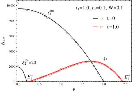
Figure 11: Localization length as a function of energy in the one-channel case. Here $t_{1}=1$, $t_{2}=0.1$, $\delta{e}=0$ and the amplitude of disorder is $W=0.1$. The solid curves are analytical results. Black curves correspond to uncoupled chains. The red one corresponds to the upper polariton (conduction) band (propagating channel) for strong coupling $t=1$, which is obtained by omitting the lower polariton (valence) band (evanescent channel). The squares and circles are data of the numerical transfer matrix. The quantitative agreement is significant except for the anomalous energy $E\simeq 1.0$, which correspands to the commesurate combination of wave vectors $4k_{1}=2\pi$. The coincidence between analytics and numerics confirms that the evanescent channel is decoupled to the propagating channel in weak disorder limit.

We specifically analyze the typical behavior of the enhancement factor $r_{1}(E)$ close to the band-edge $E_{2}^{+}$ in the case of $t<t_{c}$, where the system switch from one to two propagating channels. From Eqs. (12) and (18) it is not hard to obtain: at the band edge $E_{2}^{+}$, when coupling is weak $r_{1}(E_{2}^{+})$ deviates from $1$ like

$$1-r_{1}(E_{2}^{+})\propto\left(\frac{t}{E_{2}^{+}}\right)^{2}.$$ (135)

If $E$ is away from $E_{2}^{+}$, $r_{1}(E)$ increases linearly, i.e.,

$$r_{1}(E)-r_{1}(E_{2}^{+})\propto t^{2}(E-E_{2}^{+}),$$ (136)

with a fixed but weak coupling $t$. A typical curve for $r_{1}(E)$ is shown in the upper right insert in Fig. 6.

VII Shape and polarization of the wavefunctions

In certain applications, such as exciton-polaritons, the two linearly coupled types of excitations (represented by the two chains) are very different in nature. This makes it in principle possible to probe the original excitations separately from each other. For a two-leg atomic chain one can imagine probing the amplitude of wave function on each of the spatially separated legs. For polaritons the analogue would be a separate probing of cavity photons or excitons, e.g. by studying the 3D light emitted due to diffraction of cavity photons at surface roughnesses or by studying the exciton annihilation radiation or the electric current of exciton decomposition provoked locally. Therefore it is of practical interest to be able to manipulate the strength of localization of one of the original excitations by coupling them to the other.

VII.1 Numerical analysis

With this goal in mind we have carried out a numerical study of the amplitude of wave functions on either of the chains in each of the distinct parameter regimes discussed above. We numerically diagonalized the Hamiltonian (1), cf. Fig. 12, choosing $t_{1}=1$, $t_{2}=0.2$, $W=0.4$, $t=0.04$. The length of the ladder was taken to be $L=10^{3}$ and periodic boundary conditions were used. With the above parameters the localization lengths of the decoupled legs were of the order of $\xi_{1}^{(0)}\sim 10^{3}$ and $\xi_{2}^{(0)}\sim 10$, for energies close to the band-center. In Fig. 12 the black curves depict the amplitudes of eigenfunctions on the fast leg $1$, while the red curves show the corresponding amplitudes on the slow leg $2$.

Our main findings are:

(i) $E_{2}^{+}<E<E_{1}^{+}$: The energy is far from resonance, and only one channel exists. As shown in Fig. 12(a), most of the weight is on the fast leg. The amplitude on the slow leg is small but the spatial extension of the component $\psi_{2}$ is the same as that of $\psi_{1}$ on the fast leg, which is almost unaffected by the chain coupling. Thus the coupling can create a nonzero amplitude on the chain 2, in the energy region where the decoupled chain 2 cannot support any excitations. The spacial extension is controlled by the localization properties of the leg 1.
(ii) $t/\kappa(t_{1},t_{2})<E<E_{2}^{+}$: The energy is in the two-channel, off-resonant regime. The wavefunction components $\psi_{1}$ and $\psi_{2}$ are characterized by both localization lengths $\xi_{1}$ and $\xi_{2}$. However, the relative weights of the parts of the wavefunction with the smaller and the larger localization lengths fluctuate very strongly from eigenstate to eigenstate. This is shown in Fig. 12(b) and (c), with two adjacent energy levels, which were properly selected. In Fig. 12(b), $\psi_{2}$ consists almost entirely of a component with the smaller localization length, while the fast leg clearly shows contributions of both components. In Fig. 12(c), both $\psi_{1}$ and $\psi_{2}$ consist almost entirely of a component with the larger localization length. In brief, the former can be thought of as a state on leg 2, which weakly admixes some more delocalized states on leg 1, while the latter wavefunction is essentially a state of leg 1 which admixes several more strongly localized states on leg 2.

We have checked in specific cases that this interpretation is indeed consistent (see Sec. VII.2): In the off-resonant regime the wavefunctions can be obtained perturbatively in the coupling $t$, confirming the picture of one-leg wavefunctions with small admixtures of wavefunctions on the other leg. Off resonance, the perturbation theory is controlled even for appreciable $t$, since the matrix elements that couple wavefunctions of similar energy are very small due to significant cancellations arising from the mismatched oscillations of the wavefunctions ($k_{1}-k_{2}>\xi_{2}^{(0)}$) on the two legs. Resonance occurs precisely when at a fixed energy $k_{1}-k_{2}$ becomes too small, so that the modes on both legs start to mix strongly. A closer analysis of the perturbation theory in special cases shows that the perturbative expansion is expected to break down at the resonant crossover determined further above.

(iii) $|E|<t/\kappa(t_{1},t_{2})$: If the energy is in the resonant regime, the two localization lengths are of the same order $\xi_{1}\sim\xi_{2}\sim\xi^{(0)}_{2}$ and the spatial extension of both wave function components is governed by the localization length $\xi_{2}^{(0)}$ of the decoupled slow chain. This is illustrated in Fig. 12(d).

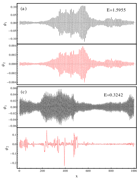
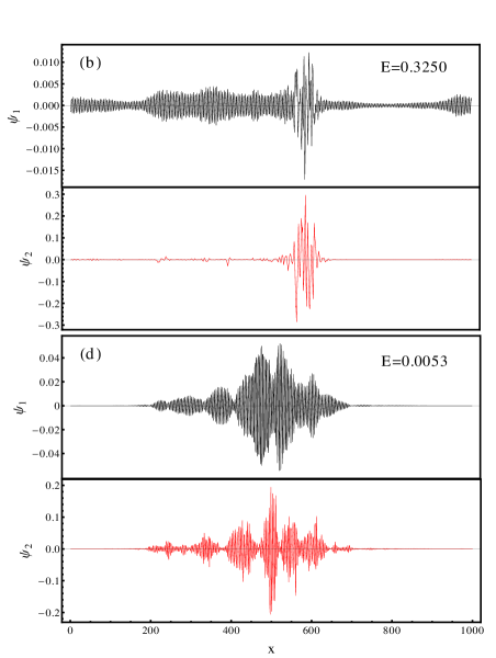
Figure 12: Typical wavefunctions in different regimes. Pay attention to the varying scales for the amplitudes in the various cases. Parameters are $t_{1}=1$, $t_{2}=0.2$, $W=0.4$, $t=0.04$, while $E$ selects the regime. The length of the ladder is $L=10^{3}$ with periodic boundary condition. The black(red) curves are the amplitudes on the 1(2)-leg. (a) $E=1.5955$, at which only one channel exist. (b) and (c) off-resonant regime: $E=0.3250$ and $E=0.3242$ are a pair of adjacent levels of ”opposite type”. (d) $E\simeq 0$, which is within the resonant regime.

VII.2 Perturbative analysis

The properties of eigenstates at different energy regimes can be explained by applying a perturbative analysis on the coupling $t$. First, we define the relevant quantities of decoupled legs as follows: the eigenstate of the $\nu$-leg with eigenenergy $E_{\nu n}$ is $\psi_{\nu n}(x)$. The corresponding localization length is $\xi_{\nu}^{(0)}$, where we assume $\xi_{1}^{(0)}\gg\xi_{2}^{(0)}$ in order to reveal the resonance–off-resonance crossover. The mean level spacing inside the localization volume is $\Delta_{\nu}$. Because in one dimension a particle is nearly ballistic in its localization volume, which means its wavevector is nearly conserved and its amplitude is almost uniform, we introduce a simple “box” approximation on the eigenstates as the following: Inside the localization volume,

$$\psi_{\nu n}(x)\sim\frac{1}{\sqrt{\xi_{\nu}^{(0)}}}e^{ik_{\nu}x},$$ (137)

up to a random phase, in which $\xi_{\nu}^{(0)}$ and $k_{\tau}$ are the localization length and the wavevector at the energy $E_{\nu n}$. Outside the localization volume $\psi_{\nu n}(x)=0$.

Now we turn on a weak enough coupling $t$ and calculate the deviation of an energy level $E_{1n}$ on the $1$-leg. Up to second order in $t$, the deviation is

$$\delta{E}_{1n}^{(2)}=t^{2}\sum_{m}{\frac{\left|\int{dx\psi_{1n}^{\ast}(x)\psi_{2m}(x)}\right|^{2}}{E_{1n}-E_{2m}}}.$$ (138)

In order to estimate the value of $\delta{E}_{1n}^{(2)}$ by the r.h.s. of Eq. (138) we have to make clear three points:

(i) The summation is dominated by the terms with the smallest denominators, whose typical value is the mean level spacing $\Delta_{2}$.

(ii) The typical value of the integral on the numerator can be estimated by the “box” approximation introduced above, which gives

$$\int{dx\psi_{1n}^{\ast}\psi_{2m}} \sim \int_{0}^{\xi_{2}^{(0)}}{dx\psi_{1n}^{\ast}\psi_{2m}}$$ (139)

$$\sim \left[\left(k_{1}-k_{2}\right)\sqrt{\xi_{1}^{(0)}\xi_{2}^{(0)}}\right]^{-1}.$$

(iii) We should consider more carefully how many dominant terms there are in the summation. We can easily realize that a state $\psi_{1n}(x)$ on the $1$-leg can couple to about $\xi_{1}^{(0)}/\xi_{2}^{(0)}$ states $\psi_{2m}(x)$ on the $2$-leg. However, the value of the summation is different from a naive deterministic evaluation because the random signs of the denominators. If we neglect the correlation of these random signs, according to the central limit theorem, the fluctuation of $\delta{E}_{1n}^{(2)}$ is

$$\left|\delta{E}_{1n}^{(2)}\right|\sim\sqrt{\frac{\xi_{1}^{(0)}}{\xi_{2}^{(0)}}}\times\frac{t^{2}}{\xi_{1}^{(0)}\xi_{2}^{(0)}(k_{1}-k_{2})^{2}\Delta_{2}}.$$ (140)

The validity of the perturbation analysis is guaranteed if

$$\left|\delta{E}_{1n}^{(2)}\right|<\Delta_{1},$$ (141)

which means there is no level-crossing in the localization volume of the $1$-leg. To estimate the relevant quantities in Eq. (141), for simplicity we assume $t_{1}\gg t_{2}$ and $\sigma_{1}^{2}=\sigma_{2}^{2}$. If the energy $E=E_{1n}$ is close to the resonant energy $E_{R}$, according to Eq. (II.1.1) and (14), we obtain

$$\left|k_{1}-k_{2}\right|\sim\left|E-E_{R}\right|(t_{1}-t_{2})/t_{1}t_{2}.$$ (142)

The mean level spacings are

$$\Delta_{\nu}\sim t_{\nu}/\xi_{\nu}^{(0)},$$ (143)

and the localization lengths satisfy

$$\xi_{1}^{(0)}/\xi_{2}^{(0)}\sim t_{1}^{2}/t_{2}^{2}.$$ (144)

Substituting Eqs. (142), (143) and (144) to Eq. (141) we obtain the condition

$$t<\left|E-E_{R}\right|(t_{1}-t_{2})/t_{1},$$ (145)

which is consistent with the result of Eq. (85) with $t_{1}\gg t_{2}$. Therefore, Eq. (141) is essentially equivalent to the criterion for being off-resonant ($\Delta{V}>0$) at weak coupling $t$.

VIII Limit of vanishing hopping on the “slow” leg

In the present work we are particularly interested in the case where the localization lengths of the uncoupled legs are parametrically different $\xi_{1}^{(0)}\gg\xi_{2}^{(0)}$. Accordingly we refer to the two legs as the “fast” and the “slow” one, respectively. So far we have analyzed the model extensively in the limit where the disorder is weak on both legs and thus $\xi_{\nu}^{(0)}\gg 1$.

Another interesting situation is the case where the hopping strength on the slow leg vanishes $t_{2}=0$, or is weak enough. This is experimentally relevant for polariton systems in which the exciton hopping is weak as compared to the disorder potential. In this case the dimensionless disorder parameter which we introduced previously diverges $\chi_{2}^{2}\to\infty$, and formally $\xi_{2}^{(0)}=0$ even if the disorder strength on this second leg is arbitrarily small. For this reason the perturbative analysis in both of $\chi_{\nu}^{2}$ breaks down. Nevertheless, this limiting case can be solved exactly, too, but requires a different treatment which goes beyond the previous weak disorder analysis.

If $t_{2}=0$, the second leg is composed of mutually non-connected sites, which form a comb structure together with the first leg. The Schrödinger equation (4) takes the form

$$\begin{split}\begin{pmatrix}-t_{1}&0\\ 0&0\end{pmatrix}&\left[\Psi(x+1)+\Psi(x-1)\right]\\ &=\begin{pmatrix}E-{\epsilon}_{x1}&t\\ t&E-\delta{e}-{\epsilon}_{x2}\end{pmatrix}\Psi(x),\end{split}$$ (146)

where

$$\Psi(x)=\begin{pmatrix}\psi_{1}(x)\\ \psi_{2}(x)\end{pmatrix},$$ (147)

describes the amplitudes on the two legs, respectively. We obtain the effective Schrödinger equation for $\psi_{1}(x)$ by eliminating $\psi_{2}(x)$ in Eq. (146):

$$-t_{1}\left[\psi_{1}(x+1)+\psi_{1}(x-1)\right]=(E-\tilde{{\epsilon}}_{x1})\psi_{1}(x-1),$$ (148)

where

$$\tilde{{\epsilon}}_{x1}={\epsilon}_{x1}+\frac{t^{2}}{E-\delta{e}-{\epsilon}_{x2}}.$$ (149)

Note that $\tilde{{\epsilon}}_{x1}$ has the meaning of an effective disorder potential on leg 1. Furthermore, if $|{\epsilon}_{x2}|\ll|E-\delta{e}|$ Eq. (149) can be expanded as

$$\tilde{{\epsilon}}_{x1}\simeq\frac{t^{2}}{E-\delta{e}}+\left[{\epsilon}_{x1}+\frac{t^{2}}{(E-\delta{e})^{2}}{\epsilon}_{x2}\right]+O({\epsilon}^{2}).$$ (150)

The first term on the r.h.s of Eq. (150) is a homogeneous potential shift. The second term is an effective disorder potential of zero mean.

Eqs. (148) and (150) represent a single-chain problem, which can be solved exactly. The dispersion relation of the disorder-free part is determined by

$$-2t_{1}\cos{k}+\frac{t^{2}}{E-\delta{e}}=E,$$ (151)

which gives the two non-overlapping bands

$$E_{\tau}(k)=-t_{1}\cos{k}+\frac{\delta{e}}{2}-(-1)^{\tau}\sqrt{\left(t_{1}\cos{k}+\frac{\delta{e}}{2}\right)^{2}+t^{2}}.$$ (152)

Of course, this coincides with Eq. (II.1.1) for $t_{2}=0$. Using the result for a single chain Anderson modelmel we obtain the localization length as

$$1/\xi=\frac{\chi_{1}^{2}+\tilde{\chi}_{2}^{2}\tan^{2}{\gamma}}{8\sin^{2}{k}}+O(\chi_{1}^{4},\tilde{\chi}_{2}^{4}).$$ (153)

Here, the disorder on the leg 2 is measured by the dimensionless ratio

$$\tilde{\chi}_{2}=\frac{\sigma_{2}^{2}}{t_{1}^{2}},$$ (154)

$\gamma$ is the mixing angle defined in Eq. (12) with $t_{2}=0$. Comparing the result (153) with Eq. (133), which describes the one-channel case in the weak disorder limit ($W_{2}\ll t_{2}$), one sees that the two limits do not commute. This is similar to the non-commutativity of the limits of weak disorder and weak inter-chain coupling in the resonant case. Similarly as Eq. (63) the characteristic disorder energy scale is the mean level spacing in the localization volume when $t_{2}=0$, which can be estimated as

$$\delta\tilde{E}\sim t_{1}/\xi\sim\max\{\sigma_{1}^{2},\sigma_{2}^{2}\}/t_{1}.$$ (155)

A perturbative analysis in $t_{2}$ is valid only if $t_{2}\ll\delta\tilde{E}$. We expect a crossover to the regime of strong hopping on the slow leg when $t_{2}\sim\delta\tilde{E}$.

The non-commutativity of the two limits is illustrated in Fig. 13 where we compare the two analytical limits with numerical simulations at fixed disorder $W_{1}=W_{2}=0.1$ and hoppings $t_{1}=t=1$. Three values of $t_{2}$ are selected to cover the crossover from the weak disorder limit ($t_{2}\gg W_{2}$) to the limit of a slow leg with disconnected sites ($t_{2}\to 0$). Eqs. (133) and (153) are indeed seen to capture the two limits very well. Note that the localization length increases monotonically with $t_{2}$ for a fixed energy, as one may expect.

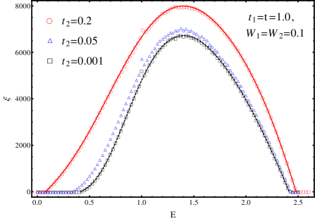
Figure 13: Localization length as a function of energy for three values of $t_{2}$. $t_{1}=t=1$ and $W_{1}=W_{2}=0.1$ are kept fixed. $t_{2}=0.2$, $0.05$ and $0.001$ capture the weak disorder limit, the intermediate regime and the limit of a nearly disconnected slow leg, respectively. The symbols are data of a numerical transfer matrix calculation. The solid and the dashed curves are the analytical results from Eqs. (133,153). The agreement with numerics in the limiting cases is very good. The localization length increases monotonically with $t_{2}$ for a fixed energy. An anomaly due to the commensurate wave vector $4k=2\pi$ appears at $E\approx 1.0$.

IX conclusion and possible applications

The most important potential application of our theory is in the realm of polaritons in quasi-one dimensional semiconductor structures tri ; man . Here the fast chain corresponds to the electromagnetic modes (”light”) confined in a one-dimensional structure and therefore having a parabolic dispersion with a very small mass (large $t_{1}$) at small wave vectors. The slow chain corresponds to the Wannier-Mott excitons, an electron-hole pair coupled by Coulomb attraction. The mass of the exciton is typically $10^{4}$ times larger than that of ”light”. Surface roughness of the one-dimensional structure and impurities therein produce a disorder potential acting on both excitons and ”light” sav . Experimentally, one can easily probe the intensity of the ”light” component by measuring the intensity of 3D photons that emerge due to diffraction from the surface roughness. The amplitude of the wavefunction of the exciton’s center-of-mass is more difficult to access, but in principle still possible, e.g. via stimulated or spontaneous exciton recombination and the related radiation. Another application is related with one-dimensional structures in cold-atom traps. By this technique one can construct and study coupled one-dimensional chains in the same way as it was recently done for a single chain Aspekt ; Roati .

While all possible regimes can be achieved in a system of cold atoms, the most relevant regime for one-dimensional cavity polaritons is that described in Fig. 1(b), where for each band (the lower and the upper polariton bands) only one channel exists. This is because the exciton-light coupling is typically stronger than the narrow bandwidth $t_{2}\sim 1/m_{\rm exc}$ of the excitons. The localization length in the case relevant for the upper exciton-polaritons is shown in Fig. 11.

As expected, the localization length tends to zero near the bottom and the top of the band, due to the vanishing rapidity. Note that in the context of polaritons the upper band edge does not exist, since the light has an unbounded continuous spectrum. In our model the top of the band appears merely due to the discreteness of the lattice. In the center of the band the localization length is of the order of the localization length for the uncoupled ”light” component. More important is the distribution of amplitudes of ”light” and ”exciton” wavefunctions which are similar to Fig. 12(a), with ”light” being represented by the wave function $\psi_{1}$ on the fast leg and the ”exciton” part being represented by the wave function $\psi_{2}$ on the slow leg. One can see that the coupling to light makes the exciton wave function spread over a distance $\xi\sim\xi^{(0)}_{1}$ of the order of the localization length of light. This is much larger than the maximum exciton localization length $\xi_{2}^{(0)}$ in the absence of coupling. The price for the ”fast transit” is that the amplitude of the exciton wave function is small. This means that the transfer of a locally created exciton to distances of order $\xi_{1}^{(0)}$ is possible, but occurs with reduced probability.

In the long search for light localization (see the paper by A. Lagendijk, B. van Tiggelen and D. S. Wiersma in Ref. fify, ) the crucial point was to achieve a smaller localization length of light. Our results show that this can also be achieved by coupling light to excitons near the bottom of the upper polariton band.

We would like to emphasize that the model considered above does not take into account an important property of polaritons, namely their finite lifetime due to recombination of excitons, and the out-coupling of the light from the waveguide. This limits the coherence of polaritons and inhibits Anderson localization. More precisely, the effects of Anderson localization are only relevant if the time to diffuse up to the scale of the localization length (which by Thouless’ argument is of the order of the inverse level spacing in the localization volume) is smaller than the life time of the excitons. Further crucial aspects are interactions among polaritons at finite density, and the related possibility of interaction-induced delocalization and Bose condensation of polaritons. marcht ; wertz A complete theory of localization of hybrid particles like polaritons should take into account all these issues.ale

Let us finally discuss the role of dimension for our results. We have found that under resonant conditions the localization lengths of two coupled chains are of the order of the localization length of the more localized, uncoupled leg. We may interpret this phenomenon as a manifestation of the fact that in 1d the mean free path is the relevant length scale that sets the localization length. Insofar it is not surprising that the backscattering rate, and thus the “worst” leg of the chains determines the localization properties of a coupled system. However, the close relation (proportionality) between mean free path and localization length is special for one-dimensional systems. In contrast in two dimensions the localization length becomes parametrically larger than the mean free path at weak disorder. In $d>2$ most eigenstates are even delocalized in weak disorder. Accordingly, we expect that the localization length is not so simply determined by the properties of the more disordered part among two coupled systems. Nevertheless, since the proliferation of weak-localization and backscattering leads to complete localization also in 2d (in the absence of special symmetries), we expect that a well propagating channel becomes more strongly localized upon resonant coupling to a more disordered channel. This may apply, e.g., to 2d polariton systems. However, in higher dimensions $d>2$ such a coupling might have a rather weak effect. We expect that a “fast” channel is not affected much by a more disordered parallel channel. That such a trend exists indeed at high enough dimensions can be shown in the case of two coupled Bethe lattices, hong-markus which can be viewed as the limit of arbitrarily high dimensions.

We leave the investigation of problems in higher dimensions, and possible implications for interacting few-particle problems for future work.

Appendix A Transfer matrix of an “elementary slice” in the current-conserving basis Eqs. (24, 26)

In this appendix we derive Eqs. (27) and (29). In Eqs. (19, 20), $\tilde{\mathbf{m}}_{x}$ is a symplectic matrix which by definition satisfies

$$\tilde{\mathbf{m}}_{x}^{T}J\tilde{\mathbf{m}}_{x}=J,$$ (156)

$$\tilde{\mathbf{m}}_{x}=\tilde{\mathbf{m}}_{x}^{*},$$ (157)

where

$$J=\begin{pmatrix}0&\mathbf{1}\\ -\mathbf{1}&0\end{pmatrix},$$ (158)

and $\tilde{\mathbf{m}}_{x}^{T}$ is the matrix obtained from $\tilde{\mathbf{m}}_{x}$ by transposition.

Define the new matrix ${\bf m}_{x}$

$${\bf m}_{x}={\bf U}_{x+1}^{-1}\,\tilde{{\bf m}}_{x}\,{\bf U}_{x},$$ (159)

where the rotation matrix is

$$\mathbf{U}_{x}\equiv\begin{pmatrix}\boldsymbol{\alpha}_{x}&\boldsymbol{\alpha}_{x}^{\ast}\\ \boldsymbol{\alpha}_{x-1}&\boldsymbol{\alpha}_{x-1}^{\ast}\end{pmatrix},$$ (160)

with $\boldsymbol{\alpha}_{x}$ defined by Eq. (28). The corresponding inverse matrix is given by:

$${\bf U}^{-1}_{x}=\frac{1}{\Delta}\begin{pmatrix}\boldsymbol{\alpha}_{x-1}^{*}&-\boldsymbol{\alpha}_{x}^{\ast}\\ -\boldsymbol{\alpha}_{x-1}&\boldsymbol{\alpha}_{x},\end{pmatrix}$$ (161)

where $\Delta$ is the diagonal matrix

$$\Delta=\boldsymbol{\alpha}_{x}\boldsymbol{\alpha}_{x-1}^{*}-\boldsymbol{\alpha}_{x}^{*}\boldsymbol{\alpha}_{x-1}.$$ (162)

The crucial point is that by current conservation Eq. (23), $\Delta$ is independent of coordinates and is proportional to the unit matrix in channel space:

$$\Delta=i\,\mathbf{1}.$$ (163)

Note also that, by construction, the rotation matrix ${\bf U}_{x}$ obeys the disorder-free Schrödinger equation Eq. (19):

$${\bf U}_{x+1}=\tilde{{\bf m}}_{x}|_{\tilde{\epsilon}=0}\,{\bf U}_{x}.$$ (164)

It follows immediately from Eqs. (164, 159) that in the absence of disorder ${\bf m}_{x}=\mathbf{1}$. In the presence of weak disorder the matrix ${\bf m}_{x}$ acquires a small coordinate-dependent correction proportional to $\tilde{\boldsymbol{\epsilon}}_{x}$ which is given by Eq. (27).

Next, by inverting Eq. (159) and plugging into Eq. (157) one obtains:

$$\boldsymbol{\Sigma}^{(1)}_{x+1}\,{\bf m}_{x}\,\boldsymbol{\Sigma}^{(1)*}_{x}={\bf m}_{x}^{*}.$$ (165)

Using definition of $\boldsymbol{\alpha}_{x}$ Eq. (28) one can readily show that

$$\boldsymbol{\Sigma}^{(1)}_{x}\equiv({\bf U}_{x}^{*})^{-1}{\bf U}_{x}=\boldsymbol{\Sigma}_{1}$$ (166)

is real and independent of $x$. This immediately reduces the time-reversal symmetry condition Eq. (165) to the form in Eq. (29).

The same procedure applied to the symplecticity relation Eq. (156) results in the following constraint (using $\tilde{\mathbf{m}}_{x}^{T}=\tilde{\mathbf{m}}_{x}^{\dagger}$):

$${\bf m}^{\dagger}_{x}\,\boldsymbol{\Sigma}^{(3)}_{x+1}\,{\bf m}_{x}=\boldsymbol{\Sigma}^{(3)}_{x},$$ (167)

where

$$\boldsymbol{\Sigma}^{(3)}_{x}\equiv{\bf U}^{\dagger}_{x}\,J\,{\bf U}_{x}=-\Delta\,\boldsymbol{\Sigma}_{3}=-i\,\boldsymbol{\Sigma}_{3}$$ (168)

is independent of coordinate due to current conservation. Thus we obtain the current conservation condition in Eq. (29).

Appendix B Perturbative calculation of $\delta{\vec{\lambda}}$ up to second order

Eqs. (38), (45) and (46) fully determine the variation of the eigen-system of the Hermitian matrix $\mathbf{R}$. It is given by $\delta{\vec{\lambda}}$, which characterize the “perturbation” $\delta{\mathbf{R}}$. We can therefore use standard perturbation theory to expand $\delta{\vec{\lambda}}$ into powers of disorder on the additional slice. In this Appendix we calculate $\delta{\vec{\lambda}}$ up to the second order, which is necessary to derive the Fokker-Planck equation (51).

We introduce some quantities which are convenient to present the results. Analogously to $\boldsymbol{\alpha}_{x}$, defined by Eq. (28), we define

$$\boldsymbol{\beta}_{x}=\boldsymbol{\alpha}_{x}\mathbf{u},$$ (169)

where $\mathbf{u}$ is the unitary matrix in Eq. (34). Since $\boldsymbol{\alpha}_{x}$ describes the propagation in the plane-wave basis on the individual chains, and $\mathbf{u}$ is the “polarization” matrix, we can consider $\boldsymbol{\beta}_{x}$ as describing clean propagation in the “polarized” plane-wave basis. Furthermore, analogously to the blocks in Eq. (27), we can define two quantities on the “polarized” basis, related with the forward- and back-scattering of the right-moving particle off the slice:

$$\begin{split}\boldsymbol{\Lambda}_{x}&=i\boldsymbol{\beta}^{\dagger}_{x}\tilde{\boldsymbol{\epsilon}}_{x}\boldsymbol{\beta}_{x},\\ \boldsymbol{\Sigma}_{x}&=i\boldsymbol{\beta}^{\dagger}_{x}\tilde{\boldsymbol{\epsilon}}_{x}\boldsymbol{\beta}_{x}^{\ast},\end{split}$$ (170)

which are $2\times 2$ matrices. It is easy to realize that $\boldsymbol{\Lambda}_{x}$ is anti-Hermitian and $\boldsymbol{\Sigma}_{x}$ is symmetric. The corresponding left-moving quantities are complex conjugates of them. The perturbative series of $\delta{\vec{\lambda}}$ are functions of elements of $\boldsymbol{\Lambda}_{x}$ and $\boldsymbol{\Sigma}_{x}$. For simplicity of further notations, we define

$$\tilde{\mathbf{F}}=\sqrt{\mathbf{F}^{2}-1},$$ (171)

and

$$\Delta{F}=F_{1}-F_{2}.$$ (172)

In order to facilitate the perturbative calculation, we adopt a parametrization of $\mathbf{R}+\delta\mathbf{R}$ as in (38), but with $\mathbf{F}\to\mathbf{F}+\delta\mathbf{F}$, $\tilde{\mathbf{F}}\to\tilde{\mathbf{F}}+\delta\tilde{\mathbf{F}}$ and $\mathbf{u}\to\mathbf{u}+\delta\mathbf{u}$, in which

$$\delta\tilde{\mathbf{F}}=\sqrt{(\mathbf{F}+\delta{\mathbf{F}})^{2}-1}-\sqrt{\mathbf{F}^{2}-1}.$$ (173)

Substituting this into Eq. (46) and (45) we obtain two coupled equations for $\delta\mathbf{F}$ and the $2\times 2$ matrix $\bf S$ which captures the incremental change of the polarization basis,

$$\mathbf{S}=1+\mathbf{u}^{\dagger}\delta{\mathbf{u}},$$ (174)

as

$$\mathbf{S}(\mathbf{F}+\delta\mathbf{F})\mathbf{S}^{\dagger}=\mathbf{F}+\mathbf{F}^{(1)}+\mathbf{F}^{(2)},$$ (175a)

$$\mathbf{S}(\tilde{\mathbf{F}}+\delta\tilde{\mathbf{F}})\mathbf{S}^{T}=\tilde{\mathbf{F}}+\tilde{\mathbf{F}}^{(1)}+\tilde{\mathbf{F}}^{(2)},$$ (175b)

We have introduced perturbation terms on the r.h.s. of the two equations as

$$\mathbf{F}^{(1)}=-\mathbf{F}\mathbf{\Lambda}_{L}+\mathbf{\Lambda}_{L}\mathbf{F}+\mathbf{\Sigma}_{L}\tilde{\mathbf{F}}+\tilde{\mathbf{F}}\mathbf{\Sigma}_{L}^{\ast},$$ (176a)

$$\mathbf{F}^{(2)}=-\mathbf{\Lambda}_{L}\mathbf{F}\mathbf{\Lambda}_{L}+\mathbf{\Sigma}_{L}\mathbf{F}\mathbf{\Sigma}_{L}^{\ast}+\mathbf{\Lambda}_{L}\tilde{\mathbf{F}}\mathbf{\Sigma}_{L}^{\ast}-\mathbf{\Sigma}_{L}\tilde{\mathbf{F}}\mathbf{\Lambda}_{L},$$ (176b)

$$\tilde{\mathbf{F}}^{(1)}=-\tilde{\mathbf{F}}\mathbf{\Lambda}_{L}^{\ast}+\mathbf{\Lambda}_{L}\tilde{\mathbf{F}}+\mathbf{\Sigma}_{L}\mathbf{F}+\mathbf{F}\mathbf{\Sigma}_{L},$$ (176c)

$$\tilde{\mathbf{F}}^{(2)}=-\mathbf{\Lambda}_{L}\tilde{\mathbf{F}}\mathbf{\Lambda}_{L}^{\ast}+\mathbf{\Sigma}_{L}\tilde{\mathbf{F}}\mathbf{\Sigma}_{L}+\mathbf{\Lambda}_{L}\mathbf{F}\mathbf{\Sigma}_{L}-\mathbf{\Sigma}_{L}\mathbf{F}\mathbf{\Lambda}_{L}^{\ast},$$ (176d)

where $\mathbf{F}^{(1)}$ and $\tilde{\mathbf{F}}^{(1)}$ are linear in disorder, while $\mathbf{F}^{(2)}$ and $\tilde{\mathbf{F}}^{(2)}$ are quadratic. Additionally, $\mathbf{F}^{(1)}$ and $\mathbf{F}^{(2)}$ are Hermitian, but $\tilde{\mathbf{F}}^{(1)}$ and $\tilde{\mathbf{F}}^{(2)}$ are symmetric.

We expand $\delta{\mathbf{F}}$ and $\delta\mathbf{u}$ in disorder strength. From the latter we calculate the corresponding variations of angular variables. Without going into the details of the calculation, we present the results up to the second order in disorder.

To first order the corrections

$$\delta{\vec{\lambda}}^{(1)}=(\delta{F}_{1}^{(1)},\delta{F}_{2}^{(1)},\delta{\theta}^{(1)},\delta{\psi}^{(1)},\delta{\phi}^{(1)},\delta{\varphi}^{(1)})$$ (177)

are given by

$$\delta{F}_{\varrho}^{(1)}=\mathbf{F}^{(1)}_{\varrho,\varrho},\quad\varrho\in\{1,2\},$$ (178a)

$$\delta{\theta}^{(1)}=\frac{2}{\Delta{F}}\text{Re}{\left(\mathbf{F}^{(1)}_{2,1}e^{i\psi}\right)},$$ (178b)

$$\delta{\psi}^{(1)}=\frac{1}{2}\left(\frac{\text{Im}\tilde{\mathbf{F}}^{(1)}_{2,2}}{\tilde{F}_{2}}-\frac{\text{Im}\tilde{\mathbf{F}}^{(1)}_{1,1}}{\tilde{F}_{1}}\right)-\delta{\varphi}^{(1)}\cos{\theta},$$ (178c)

$$\delta{\phi}^{(1)}=-\frac{1}{2}\left(\frac{\text{Im}\tilde{\mathbf{F}}^{(1)}_{2,2}}{\tilde{F}_{2}}+\frac{\text{Im}\tilde{\mathbf{F}}^{(1)}_{1,1}}{\tilde{F}_{1}}\right),$$ (178d)

$$\delta{\varphi}^{(1)}=\frac{2}{\Delta{F}}\text{Im}{\left(\mathbf{F}^{(1)}_{2,1}e^{i\psi}\right)}\csc{\theta},$$ (178e)

where the subscripts denote the matrix elements of the “perturbations” $\mathbf{F}^{(1)}$ in Eq. (178). We recall that the “perturbations” in Eq. (178) are $L$-dependent.

The second order corrections

$$\delta{\vec{\lambda}}^{(2)}=(\delta{F}_{1}^{(2)},\delta{F}_{2}^{(2)},\delta{\theta}^{(2)},\delta{\psi}^{(2)},\delta{\phi}^{(2)},\delta{\varphi}^{(2)})$$ (179)

are more complicated. However, we recall that our aim is to calculate the correlators $\overline{\delta{\lambda_{i}^{(1)}}\delta{\lambda_{j}^{(1)}}}$ and $\overline{\delta{\lambda_{i}^{(2)}}}$ in Eq. (51). To avoid repeating calculation, we should express the $\delta{\vec{\lambda}}^{(2)}$’s in terms of the first order corrections Eq. (178) as far as possible. We obtain

$$\delta{F}_{\varrho}^{(2)}=\mathbf{F}^{(2)}_{\varrho,\varrho}-(-1)^{\varrho}\frac{|\mathbf{F}^{(1)}_{2,1}|^{2}}{\Delta{F}},\quad\varrho\in\{1,2\},$$ (180a)

$$\delta{\theta}^{(2)}=\frac{2}{\Delta{F}}\text{Re}{\left(\mathbf{F}^{(2)}_{2,1}e^{i\psi}\right)}+a^{(1)}\delta{\theta}^{(1)}+\frac{1}{4}\sin{2\theta}\left(\delta{\varphi}^{(1)}\right)^{2},$$ (180b)

$$\delta{\psi}^{(2)}=a^{(2)}_{-}+b^{(1)}_{-}\delta{\phi}^{(1)}+b_{+}^{(1)}d^{(1)}+c_{+}e^{(2)}-a^{(1)}_{-}c^{(1)}_{+}-\frac{1}{2}\sin{\theta}\delta{\theta}^{(1)}\delta{\varphi}^{(1)}-\cos{\theta}\delta{\varphi}^{(2)},$$ (180c)

$$\delta{\phi}^{(2)}=-a_{+}^{(2)}-b_{+}^{(1)}\delta\phi^{(1)}-b_{-}^{(1)}d^{(1)}+c_{-}e^{(2)},$$ (180d)

$$\delta{\varphi}^{(2)}=\frac{2}{\Delta{F}}\text{Im}{\left(\mathbf{F}^{(2)}_{2,1}e^{i\psi}\right)}\csc{\theta}+a^{(1)}\delta{\varphi}^{(1)}-\cot{\theta}\delta\theta^{(1)}\delta\varphi^{(1)},$$ (180e)

in which

$$a^{(1)}=\frac{1}{\Delta{F}}\left(\delta{F}_{2}^{(1)}-\delta{F}_{1}^{(1)}\right),$$ (181a)

$$a^{(2)}_{\pm}=\frac{1}{2}\left(\frac{\text{Im}\tilde{\mathbf{F}}^{(2)}_{2,2}}{\tilde{F}_{2}}\pm\frac{\text{Im}\tilde{\mathbf{F}}^{(2)}_{1,1}}{\tilde{F}_{1}}\right),$$ (181b)

$$b_{\pm}^{(1)}=\frac{1}{2}\left(\frac{F_{1}}{\tilde{F}_{1}^{2}}\delta{F}_{1}^{(1)}\pm\frac{F_{2}}{\tilde{F}_{2}^{2}}\delta{F}_{2}^{(1)}\right),$$ (181c)

$$c_{\pm}=\frac{1}{2}\left(\frac{\tilde{F}_{1}}{\tilde{F}_{2}}\pm\frac{\tilde{F}_{2}}{\tilde{F}_{1}}\right),$$ (181d)

$$d^{(1)}=\delta\varphi^{(1)}\cos{\theta}+\delta\psi^{(1)},$$ (181e)

$$e^{(2)} = \frac{1}{4}\left[\left(\delta\varphi^{(1)}\right)^{2}\sin^{2}{\theta}-\left(\delta\theta^{(1)}\right)^{2}\right]\sin{2\psi}$$ (181f)

$$+\frac{1}{2}\delta\varphi^{(1)}\delta\theta^{(1)}\sin{\theta}\cos{2\psi}.$$

In practice, we first calculate all the correlators $\overline{\delta{\lambda_{i}^{(1)}}\delta{\lambda_{j}^{(1)}}}$ by Eq. (178). At the same time we obtain the correlators relevant for the products of first order terms on the r.h.s. of Eq. (180). Finally, after evaluating the disorder average of $a^{(2)}_{\pm}$ in Eq. (181b), $\overline{\delta{\lambda_{i}^{(2)}}}$s can be obtained.

Appendix C co-efficients of Eq. (68)

The co-efficients of Eq. (68) are

$$c_{1}=-2\frac{\tilde{F}_{1}^{2}}{\Delta{F}}\Gamma_{6},$$ (182a)

$$c_{2}=2\frac{\tilde{F}_{2}^{2}}{\Delta{F}}\Gamma_{6},$$ (182b)

$$c_{3}= \frac{1}{\Delta{F}^{2}}\left[\left(F_{1}^{2}-F_{2}^{2}-2\right)\left(\Gamma_{5}+\Gamma_{4}\right)+2F_{1}F_{2}\left(\Gamma_{5}-\Gamma_{4}\right)\right.$$ (182c)

$$\left.-\left(\tilde{F}_{1}^{2}+\tilde{F}_{2}^{2}\right)\left(1-u^{2}\right)\partial_{u}\Gamma_{6}\right]-4\frac{1}{\Delta{F}^{2}}\tilde{F}_{1}\tilde{F}_{2}u\Gamma_{6}\cos{2\psi},$$

$$c_{4}= \frac{1}{\Delta{F}}\left[\left(\tilde{F}_{1}\tilde{F}_{2}+\frac{F_{2}}{\tilde{F}_{2}}\tilde{F}_{1}-\frac{F_{1}}{\tilde{F}_{1}}\tilde{F}_{2}\right)\Gamma_{3}+2\frac{\tilde{F}_{1}\tilde{F}_{2}}{\Delta{F}}\frac{u}{\sqrt{1-u^{2}}}\left(\Gamma_{5}-\Gamma_{4}\right)\right.$$ (182d)

$$\left.+\frac{F_{1}}{\tilde{F}_{1}}\tilde{F}_{2}\partial_{u}\Gamma_{4}+\frac{F_{2}}{\tilde{F}_{2}}\tilde{F}_{1}\partial_{u}\Gamma_{5}-2\frac{\tilde{F}_{1}\tilde{F}_{2}}{\Delta{F}}\left(\Gamma_{6}+2u\partial_{u}\Gamma_{6}\right)\right]\sin{2\psi},$$

$$c_{11}=\tilde{F}_{1}^{2}\Gamma_{1},$$ (182e)

$$c_{12}=2\tilde{F}_{1}\tilde{F}_{2}\Gamma_{3}\cos{2\psi},$$ (182f)

$$c_{13}=\frac{2\tilde{F}_{1}}{\Delta{F}}\left(\tilde{F}_{1}+\tilde{F}_{2}\cos{2\psi}\right)\Gamma_{4},$$ (182g)

$$c_{14}=-\tilde{F}_{1}\left(\frac{F_{2}}{\tilde{F}_{2}}\Gamma_{3}+2\frac{\tilde{F}_{2}}{\Delta{F}}\frac{u}{\sqrt{1-u^{2}}}\Gamma_{4}\right)\sin{2\psi},$$ (182h)

$$c_{22}=\tilde{F}_{2}^{2}\Gamma_{2},$$ (182i)

$$c_{23}=2\frac{\tilde{F}_{2}}{\Delta{F}}\left(\tilde{F}_{2}+\tilde{F}_{1}\cos{2\psi}\right)\Gamma_{5},$$ (182j)

$$c_{24}=-\tilde{F}_{2}\left(\frac{F_{1}}{\tilde{F}_{1}}\Gamma_{3}+2\frac{\tilde{F}_{1}}{\Delta{F}}\frac{u}{\sqrt{1-u^{2}}}\Gamma_{5}\right)\sin{2\psi},$$ (182k)

$$c_{33}=\left[V_{3}+\frac{1}{\Delta{F}^{2}}\left(\tilde{F}_{1}^{2}+\tilde{F}_{2}^{2}+2\tilde{F}_{1}\tilde{F}_{2}\cos{2\psi}\right)\Gamma_{6}\right]\left(1-u^{2}\right),$$ (182l)

$$c_{34}=-\frac{1}{\Delta{F}}\left(\frac{F_{1}\tilde{F}_{2}}{\tilde{F}_{1}}\Gamma_{4}+\frac{\tilde{F}_{1}F_{2}}{\tilde{F}_{2}}\Gamma_{5}-4\frac{\tilde{F}_{1}\tilde{F}_{2}}{\Delta{F}}u\Gamma_{6}\right)\sin{2\psi},$$ (182m)

$$\begin{split}c_{44}=&\frac{1}{2}\left[1+\frac{1}{2}\left(\frac{F_{1}}{\tilde{F}_{1}}\right)^{2}\right]\Gamma_{1}+\frac{1}{2}\left[1+\frac{1}{2}\left(\frac{F_{2}}{\tilde{F}_{2}}\right)^{2}\right]\Gamma_{2}-\Gamma_{6}\\ &+\frac{u}{\sqrt{1-u^{2}}}\left[\left(2+\frac{F_{1}}{\Delta{F}}\right)\Gamma_{4}+\left(2+\frac{F_{2}}{\Delta{F}}\right)\Gamma_{5}\right]+\frac{u^{2}}{1-u^{2}}\left[\Gamma_{3}+\left(1+\frac{\tilde{F}_{1}^{2}+\tilde{F}_{2}^{2}}{\Delta{F}^{2}}\right)\Gamma_{6}\right]\\ &-\left[\frac{1}{2}\frac{F_{1}F_{2}}{\tilde{F}_{1}\tilde{F}_{2}}\Gamma_{3}+\frac{u}{\sqrt{1-u^{2}}}\frac{1}{\Delta{F}}\left(\frac{F_{1}\tilde{F}_{2}}{\tilde{F}_{1}}\Gamma_{1}+\frac{\tilde{F}_{1}F_{2}}{\tilde{F}_{2}}\Gamma_{2}\right)+2\frac{u^{2}}{1-u^{2}}\frac{\tilde{F}_{1}\tilde{F}_{2}}{\Delta{F}^{2}}\right]\cos{2\psi},\end{split}$$ (182n)

where the $\tilde{F}_{\varrho}$’s are the two diagonal elements of the matrix (171) and $\Delta{F}$ is defined in Eq. (172). The new quantities introduced in Eq. (C) are defined below. Notice first that The $\Gamma_{n}$ are functions of $u$ defined by

$$\Gamma_{1(2)}(u)=V_{1}+V_{2}+4V_{3}-(+)2\left(V_{2}-V_{1}\right)u+\left(V_{1}+V_{2}-4V_{3}\right)u^{2},$$ (183a)

$$\Gamma_{3}(u)=\left(V_{1}+V_{2}-4V_{3}\right)\left(1-u^{2}\right),$$ (183b)

$$\Gamma_{4(5)}(u)=\left[V_{1}-V_{2}+(-)\left(V_{1}+V_{2}-4V_{3}\right)u\right]\left(1-u^{2}\right),$$ (183c)

$$\Gamma_{6}(u)=V_{1}+V_{2}-\left(V_{1}+V_{2}-4V_{3}\right)u^{2},$$ (183d)

where $V_{1}$, $V_{2}$ and $V_{3}$ are the three Born cross-sections defined in Eq. (60). In order to solve Eq. (78) in the limit $L\gg 1$, we need the values of $c_{3}$ and $c_{33}$ in the limit $F_{\max}\gg F_{\min}\gg 1$,

$$\lim_{L\rightarrow\infty}c_{3}=\left(\left|V_{1}-V_{2}\right|-\partial_{u}\Gamma_{6}\right)(1-u^{2}),$$ (184)

$$\lim_{L\rightarrow\infty}c_{33}=\left(V_{3}+\Gamma_{6}\right)\left(1-u^{2}\right),$$

which is Eq. (79).

Appendix D Transfer matrix of an “elementary slice” in the basis Eqs. (24, 107)

The derivation of Eq. (108) goes in parallel with the derivation of Eq. (27) in App. A. However, the rotation $\mathbf{U}_{x}$ is constructed in such a way that

$$\mathbf{U}_{x}=\begin{pmatrix}\psi_{1}^{+}(x)&\psi_{1}^{-}(x)&0&0\\ 0&0&\psi_{2}^{+}(1)&\psi_{2}^{-}(1)\\ \psi_{1}^{+}(x-1)&\psi_{1}^{-}(x-1)&0&0\\ 0&0&\psi_{2}^{+}(0)&\psi_{2}^{-}(0)\end{pmatrix},$$ (185)

where $\psi_{1,2}^{\pm}(x)$ are defined by Eqs. (24) and (107). Compared with Eq. (160) for the two-channel case, the second and third columns of Eq. (185) have been permuted, and the columns corresponding to the evanescent channel are coordinate-independent. The inverse of $\mathbf{U}_{x}$ is

$$\mathbf{U}_{x}^{-1}=\begin{pmatrix}-i\psi_{1}^{-}(x-1)&0&i\psi_{1}^{-}(x)&0\\ i\psi_{1}^{+}(x-1)&0&-i\psi_{1}^{+}(x)&0\\ 0&-\psi_{2}^{-}(0)&0&\psi_{2}^{-}(1)\\ 0&\psi_{2}^{+}(0)&0&-\psi_{2}^{+}(1)\end{pmatrix}.$$ (186)

The transfer matrix of an elementary slice (108) is

$$\begin{split}\mathbf{m}_{x}=&\mathbf{U}_{x+1}^{-1}\tilde{\mathbf{m}}_{x}\mathbf{U}_{x}=\mathbf{m}+\delta{\mathbf{m}}_{x},\end{split}$$ (187)

where $\mathbf{m}$ and $\delta{\mathbf{m}}_{x}$ take the form given in Eq. (109). Following the same procedure as in App. A, one can also obtain the symmetry constraints on the matrix $\mathbf{m}_{x}$, which is imposed by the reality and symplecticity of the matrix $\tilde{\mathbf{m}}_{x}$. Without going into details we present the following results: The reality relation (157) gives

$$\mathbf{m}_{x}^{\ast}=\boldsymbol{\Lambda}_{1}\mathbf{m}_{x}\boldsymbol{\Lambda}_{1},\quad\boldsymbol{\Lambda}_{1}=\begin{pmatrix}\sigma_{1}&0\\ 0&\mathbf{1}\end{pmatrix};$$ (188)

The symplecticity relation (156) gives

$$\mathbf{m}_{x}^{\dagger}\boldsymbol{\Lambda}_{3}\mathbf{m}_{x}=\boldsymbol{\Lambda}_{3},\quad\boldsymbol{\Lambda}_{1}=\begin{pmatrix}\sigma_{3}&0\\ 0&\sigma_{2}\end{pmatrix}.$$ (189)

Finally, it is not hard to show that the Lyapunov exponents of the products (30) satisfy the symmetry property stated in Eq. (114).

- (1) P. W. Anderson, Phys. Rev. 109, 1492 (1958).
- (2) 50 years of Anderson localization, ed. by E. Abrahams, World Scientific, 2010.
- (3) E. Abrahams, P. W. Anderson, D. C. Licciardello, and T. V. Ramakrishnan, Phys. Rev. Lett. 42, 673 (1979).
- (4) V. L. Berezinskii, Zh. Exp. Tero. Fiz. 65, 1251 (1973) [Sov. Phys. JETP 38, 620 (1974)].
- (5) V. I. Mel’nikov, Fiz. Tverd. Tela (Leningrad) 23, 782 (1981) [Sov. phys. Solid State 23, 444 (1981)].
- (6) K. B. Efetov, Supersymmetry in disorder and chaos, Cambridge University Press, 1999.
- (7) M. E. Gertsenshtein and V. B. Vasil’ev, Theor. Probab. Appl., IV, 391 (1959).
- (8) O. N. Dorokhov, Solid State Commun. 44, 915 (1982).
- (9) M. Kasner and W. Weller, Phys. Stat. Solidi (b) 148, 635 (1988).
- (10) A. V. Tartakovski, Phys. Rev. B 52, 2704 (1995).
- (11) P. A. Mello, P. Pereyra and N. Kummar, Ann. Phys. 181, 290 (1988).
- (12) P. A. Mello and N. Kumar, Quantum Transport in Mesoscopic Systems: Complexity and Statistical Fluctuations (Oxford University Press, 2004).
- (13) C. W. J. Beenakker and B. Rejaei, Phys. Rev. Lett. 71, 3689 (1993); Phys. Rev. B 49, 7499 (1994).
- (14) A. Trichet et al. Phys. Rev. B 83, 041302(R) (2011).
- (15) F. Manni, et al. Phys. Rev. Lett. 106, 176401 (2011).
- (16) V. Savona, et al. Phys. Rev. Lett. 78, 4470 (1997).
- (17) V. A. Kosobukin, Fiz. Tverd. Tela 45(6), 1091 (2003) [Phys. Solid State 45(6), 1145 (2003)].
- (18) D. M. Whittaker, et al. Phys. Rev. Lett. 77, 4792 (1996).
- (19) W. Zhang, et al. Phys. Rev. B 81, 214202 (2010).
- (20) A. U. Thomann, V. B. Geshkenbein and G. Blatter, Phys. Rev. B 79, 184515 (2009).
- (21) M. Hamermesh, Group Theory and This Applications to Physical Problem, (Addison-Wesley, 1962).
- (22) V. E. Kravtsov and V. I. Yudson, Phys. Rev. B 82, 195120 (2010); Annals of Physics, 326, 1672 (2011).
- (23) B. P. Nguyen and K. Kim, J. Phys.: Cond. Matter 24, 135303 (2012).
- (24) The transmission matrix we calculate here describes transmission from left to right of the sample. Its transpose describes the reverse transmission, as assured by time reversal symmetry. Its element denotes the out-going amplitude on the r.h.s of the sample in the -channel when there is a unit current incident from the l.h.s in the -channel.
- (25) Z. Shi and A. Z. Genack, Phys. Rev. Lett. 108, 043901 (2012).
- (26) S. Fishman, D. R. Grempel and R. E. Prange, Phys. Rev. Lett. 49, 509 (1982).
- (27) A. MacKinnon and B. Kramer, Z. Phys. B 53, 1 (1983); A. MacKinnon, in Anderson Localization and Its Ramifications: Disorder, Phase Coherence and Electron Correlations [Lect. Notes Phys. Vol. 630], edited by T. Brandes and S. Kettemann (Springer, 2003), p. 21.
- (28) P. F. Bagwell, Phys. Rev. B 41, 10354 (1990).
- (29) J. Heinrichs, Phys. Rev. B 68, 155403 (2003).
- (30) Repeating the perturbative calculation in App. B, we can obtain three cross-sections similar to Eq. (60), in which and acquire exponential growing factors and . Thus the obstacle of divergence can be rephrased in this way: The intensities of intra-evanescent-channel and inter-channel scattering (either forward or backward) are amplified exponentially with respect to the coordinate of the elementary slice, which invalidates the weak disorder expansion of .
- (31) G. Benettin, L. Galgani, A. Giorgilli, J. M. Strelcyn, Meccanica 15, 9,21 (1980); A. Crisanti, G. Paladin, A. Vulpiani, Products of Random Matrices in Statistical Physics [Springer Series in Solid-State Sciences 104], (Springer-Verlag, 1993).
- (32) J. H. Davies, The Physics of Low-Dimensional Semiconductors: An Introduction, (Cambridge University Press, 1998).
- (33) H. Huang and S. W. Koch, Quantum Theory of the Optical and Electronic Properties of Semiconductors, (World Scientific, 2004).
- (34) J. Billy, V. Josse, Z. Zuo, A. Bernard, B. Hambrecht, P. Lugan, D. Clement, L. Sanchez-Palencia, P. Bouyer, and A. Aspect, Nature (London), 453, 891 (2008).
- (35) G. Roati, C. D’Errico, L. Falani, M. Fattori, C. Fort, M. Zaccanti, G. Modugno, M. Modugno, and M. Inguscio, Nature (London), 453, 895 (2008).
- (36) F. M. Marchetti, J. Keeling, M. H. Szymańska and P. B. Littlewood, Phys. Rev. B 76, 115326 (2007).
- (37) E. Wertz, L. Ferrier, D. D. Solnyshkov, R. Johne, D. Sanvitto, A. Lemaître, I. Sagnes, R. Grousson, A. V. Kavokin, P. Senellart, G. Malpuech and J. Bloch, Nature Phys. 6, 860 (2010).
- (38) Note that we are using the semiconductor terminology of valence and conduction band rather loosely to denote the lower and the upper energy band. They will typically not be separated by a gap, but overlap in some energy range, see Fig. 1. The latter ”two-channel regime” is at the focus of our attention in this paper.
- (39) I. L. Aleiner, B. L. Altshuler and Y. G. Rubo, Phys. Rev. B 85, 121301(R) (2012).
- (40) H. Y. Xie and M. Müller (unpublished).