Robustness Leads Close to the Edge of Chaos in Coupled Map Networks: toward the understanding of biological networks

Abstract

Dynamics in biological networks are in general robust against several perturbations. We investigate a coupled map network as a model motivated by gene regulatory networks and design systems which are robust against phenotypic perturbations (perturbations in dynamics), as well as systems which are robust against mutation (perturbations in network structure). To achieve such a design, we apply a multicanonical Monte Carlo method. Analysis based on the maximum Lyapunov exponent and parameter sensitivity shows that systems with marginal stability, which are regarded as systems at the edge of chaos, emerge when robustness against network perturbations is required. This emergence of the edge of chaos is a self-organization phenomenon and does not need a fine tuning of parameters.

1 Introduction

Complex dynamical behaviors on a network can be found in a variety of biological networks, such as gene regulatory networks, neural networks and food-web. Such systems share a common characteristic: observed dynamics are robust against disturbance introduced in its dynamics, as well as against disturbance in its network [1, 2, 3]. For example, gene expression patterns obtained thorough transcription-translation regulations are kept stable in spite of extrinsic noises (i.e., perturbations in dynamics) and mutations (i.e., perturbations in a network). It seems reasonable to think that robustness against environmental perturbations has been evolutionarily developed for adapting to noisy environments. There are also several advantages in having mutational robustness - it buffers against deleterious mutations. Recently, robustness in biological networks has attracted much attention of many researchers and has been thought to be one of fundamental properties of life [1, 2, 3, 4].

This point of view naturally gives rise to the question: what kind of system emerges when only robustness is required ? The answer to this question will be helpful for understanding the design principle of living systems. In this paper, we investigate a coupled chaotic map network motivated by gene regulatory networks and show that systems at the edge of chaos are selected with only the requirement of robustness against network perturbations.

It has long been hypothesized that living systems favor the edge of chaos, where stability and chaoticity coexist. Originally, Kauffman [5] introduced the Boolean network model (N-K model) as a model of a gene regulatory network, and proposed the hypothesis that living systems prefer the edge of chaos because it allows systems to have complex behaviors [5]. Here we propose an alternative scenario, specifically that the requirement of having robustness against network perturbations drives living systems to the edge of chaos, regardless of whether or not staying at the edge of chaos is beneficial for living systems. In other wards, the edge of chaos can emerge as a byproduct of the robustness.

2 Model

We propose a coupled map system motivated by gene regulatory networks. Unlike the N-K model, each element in this model has its own dynamics. Assuming that $x^{t}_{i}\in\{-1\leq x_{i}^{t}\leq 1\}$ is the gene expression of the i-th gene at time step $t$, the single gene dynamics are written as $x_{i}^{t+1}=G(x_{i}^{t})$. These dynamics mimic multiple processes in an expression of a single gene. In the presence of $N$ genes, the dynamics of $x_{i}^{t}$ are expressed as

$$x_{i}^{t+1}=(1-\epsilon)G(x_{i}^{t})+\epsilon\sum_{j}^{N}W_{ij}G(x_{j}^{t}),$$ (1)

where $\epsilon$ is a coupling constant. $W_{ij}$ describes the strength of the interaction acting from gene j on gene i; and $W_{ij}\in[0,1]$ satisfies both conditions $W_{ii}=0$ and $\sum_{j}^{N}W_{ij}=1$ for each $i$. We call the matrix $W$, whose $ij$ element is $W_{ij}$, a network. Here we choose the logistic map $g(x,a)=1-ax^{2}$ as $G(\cdot)$. We use the model parameters $a$ and $\epsilon$ as $(a,\epsilon)=(1.8,0.1)$. This choice indicates that a single disconnected gene exhibits chaotic dynamics. A reason of this choice of $G(\cdot)$ is that a single gene expression is expected to be complex due to multiple processes underlying it We impose an additional constraint on $W$: the number of input links $k$ to each gene is fixed. We note that in the case of $W_{ij}=1/(N-1)$ for all $(i,j)$, the system becomes the globally coupled map (GCM) [6] and it shows highly chaotic behaviors at the parameters $(a,\epsilon)=(1.8,0.1)$. In contrast to the N-K model, variables of this model take continuous values and a linear stability analysis can be applied.

In this model, the network $W$ is regarded as a genotype while the attractor of dynamics $\mbox{\boldmath$x$}^{t}$ is regarded as a phenotype. Our goal is to design networks under the two different design principles: robustness against phenotypic perturbations (i.e., perturbations in the dynamics of gene $x$) and robustness against genotypic perturbations (i.e., perturbations on network $W$). In both cases, only network $W$ is tuned.

3 Design of Robust Network Against Perturbations in Dynamics

Let us start with the first design principle, namely robustness against perturbations in dynamics. In other words, we are aiming to design a system with a stable attractor. For this end, we use Lyapunov exponent analysis and a multicanonical Monte Carlo method [7, 8].

Once a network $W$ is given, the finite time maximum Lyapunov exponent $\lambda_{1}$ [9] is calculated for the dynamical system in Eq. (1), starting from a given initial state $x^{0*}_{i}$. We perform the simulation up to $T=1500$ and regard the first $T^{\prime}=1000$ steps as transient and discard them.

Our aim here is to sample networks with negative $\lambda_{1}$, which indicates that dynamics of a network is stable. Such networks are expected to be rare for large $N$, because dynamics tend to be chaotic at the present parameters. We define the probability density of $\lambda_{1}$ as

$$D(\lambda)=\int_{0}^{1}\delta(\lambda_{1}(W)-\lambda)p(W)\ \ \Pi_{i,j}dW_{ij},$$

where $\delta$ is the Dirac $\delta$-function, and $p(W)$ is the prior probability density that a network $W$ appears under random sampling. We consider here a network ensemble in which $p(W)$ is a uniform distribution under the constraints of $W_{ii}=0$ and $\sum_{j}^{N}W_{ij}=1$, given by

$$p(W) \propto\Pi_{i}\delta(\sum_{j}W_{ij}-1)\delta(\sum_{j}\theta(W_{ij})-k)\delta(W_{ii}),$$ (2)

where $\theta(z)$ is a function that satisfies $\theta(z)=1$ for $z\neq 0$ and $\theta(z)=0$ for $z=0$.

If a random sampling method is adopted in order to sample a network with “rare” value of $\lambda_{1}$ with probability $D(\lambda_{1})$, $1/D(\lambda_{1})$ samples are required at least. If an annealing method or an steepest descent method is adopted instead, we would obtain only a network with negative $\lambda_{1}$ but could not estimate D($\lambda_{1}$), which plays a key role in the further analysis. Alternatively, we apply multicanonical Monte Carlo method [7, 10, 11], which has been used in fields of statistical physics, such as spin glass [12, 13] and other studies [14, 15]. This method allows us to sample networks with negative $\lambda_{1}$ efficiently and to estimate $D(\lambda_{1})$.

Our multicanonical Monte Carlo strategy adopted in this study is to perform random walks in $\lambda_{1}$ space by generating a Markov chain, where each step is biased inversely proportional to the probability $D(\lambda_{1})$, and thereby it enables us to obtain a flat histogram in $\lambda_{1}$ space, namely to equally sample $\lambda_{1}$ whose $D(\lambda_{1})$ are many orders of magnitude different. In order to generate the Markov chain in multicanonical Monte Carlo, a key quantity is the weight function $w(\lambda_{1})$ of $\lambda_{1}$. If we have $w(\lambda_{1})$ that is inversely proportional to $D(\lambda_{1})$, networks with various $\lambda_{1}$ value are generated one after another, using the Markov process described in the Appendix (i). As a consequence, a uniform distribution of $\lambda_{1}$ (i.e., a flat histogram of $\lambda_{1}$) is obtained. We call these procedures as “random walk in $\lambda_{1}$ space”. Details of the algorithm are given in the Appendix (i) and (ii). However, neither $w(\lambda_{1})$ nor $D(\lambda_{1})$ are known a priori. In this study, the Wang and Landau algorithm [12, 13] is used to construct and to tune the weight function $w(\lambda_{1})$. Details of the implementation are given in Appendix (ii).

Figure 1 shows the calculated densities $D(\lambda_{1})$ of $\lambda_{1}$ for the fixed input degree $k=2-5$. Using density $D(\lambda_{1})$ in Fig. 1, the probability that networks with negative $\lambda_{1}$ are observed under random sampling is calculated by $P(\lambda_{1}<0)=\int_{\lambda_{a}}^{0}D(\lambda_{1})d\lambda_{1}$. We estimate $P(\lambda_{1}<0)$ with $k=2-5$ and $k=N-1$, which are shown in Fig. 2. Each $P(\lambda_{1}<0)$ shows that a stable attractor becomes increasingly rare as $N$ or $k$ increases, indicating that these systems are in the chaotic phase (we define that a system is in the chaotic phase when only positive values of $\lambda_{1}$ appear as $N\to\infty$). These results are consistent with the behavior of GCM with $(a,\epsilon)=(1.8,0.1)$ [6].

4 Design of Robust Network Against Perturbations in Network

Using the second design principle, we design systems that are robust against genotypic perturbations (i.e., network perturbations). In other words, we design, using a multicanonical Monte Carlo method, networks $W$ whose trajectory on the attractor hardly changes when a small network perturbation $\delta W$ is added. We define the parameter sensitivity and use it as a guiding function of the robustness.

Sensitivity analysis using parameter sensitivity has been developed and applied in various fields [16, 17]. While most of these studies have dealt with continuous time systems, we define the parameter sensitivity for discrete time systems as follows.

Let us denote the set of elements in $W$ in Eq. (1) by a vector $W$. When a small network perturbation $\delta\mbox{\boldmath$W$}$ is introduced into $W$ at $t=T^{\prime}$, the displacement between unperturbed trajectory $\mbox{\boldmath$x$}^{t}(\mbox{\boldmath$W$})$ and perturbed trajectory $\mbox{\boldmath$x$}^{t}(\mbox{\boldmath$W$}+\delta\mbox{\boldmath$W$})$ is approximated by $(\partial\mbox{\boldmath$x$}^{t}/\partial\mbox{\boldmath$W$})\delta\mbox{\boldmath$W$}$, where $\partial\mbox{\boldmath$x$}^{t}/\partial\mbox{\boldmath$W$}$ is a $N\times N^{2}$ matrix. We call this matrix the sensitivity matrix $\Delta^{t}$, and the time evolution of $\Delta^{t}$ is given by

$$\Delta^{t+1}=\frac{\partial\mbox{\boldmath$F$}}{\partial\mbox{\boldmath$x$}}\Delta^{t}+\frac{\partial\mbox{\boldmath$F$}}{\partial\mbox{\boldmath$W$}},$$

where $\partial\mbox{\boldmath$F$}/\partial\mbox{\boldmath$x$}$ is the Jacobian matrix and $\partial\mbox{\boldmath$F$}/\partial\mbox{\boldmath$W$}$ is the parametric Jacobian matrix. It should be noticed that the two trajectories $\mbox{\boldmath$x$}^{t}(\mbox{\boldmath$W$})$ and $\mbox{\boldmath$x$}^{t}(\mbox{\boldmath$W$}+\delta\mbox{\boldmath$W$})$ coincide for $t\leq T^{\prime}$, and thus $\Delta^{t}=0$ for $t\leq T^{\prime}$. The growth rate of the displacement between $\mbox{\boldmath$x$}^{t}(\mbox{\boldmath$W$}+\delta\mbox{\boldmath$W$})$ and $\mbox{\boldmath$x$}^{t}(\mbox{\boldmath$W$})$ with respect to the perturbation vector $\delta\mbox{\boldmath$W$}$ is obtained by $\Delta^{t}\mbox{\boldmath$\delta\hat{W}$}$, where $\mbox{\boldmath$\delta\hat{W}$}=\delta\mbox{\boldmath$W$}/|\delta\mbox{\boldmath$W$}|$. The maximum value of $|\Delta^{t}\mbox{\boldmath$\delta\hat{W}$}|$ at time step $t$ is given by the maximum singular value $\sigma_{1}^{t}$ of $\Delta^{t}$ matrix. $\sigma_{1}^{t}$ can be obtained by performing the singular value decomposition of $\Delta^{t}$. $\sigma_{1}^{t}$ diverges for $t\to\infty$ when the maximum Lyapunov exponent of the trajectory is positive. On the other hand, $\sigma_{1}^{t}$ oscillates or converges to a constant value when the maximum Lyapunov exponent is negative. Note that no parameters except for $W$ are perturbed in this study. Once a network $W$ is given, $\Delta^{t}$ and its $\sigma_{1}^{t}$ are estimated for each time step. We define parameter sensitivity $\gamma$ as the logarithm of an average of $\sigma_{1}^{t}$ along the trajectory:

$$\gamma=\ln\left(\frac{\sum_{t=T^{\prime}}^{T_{max}-1}\sigma_{1}^{t}}{T_{max}-T^{\prime}}\right).$$

Here, we regard the first $T^{\prime}-1$ steps of the trajectory as transient, and discard them. We use $T^{\prime}=1000$ and $T_{max}=1500$.

Our goal is to sample networks with small $\gamma$. However, networks with positive $\lambda_{1}$ tend to have large $\gamma$. For this reason, and because almost all networks sampled by random sampling should have positive $\lambda_{1}$, random sampling is not suitable for the sampling of networks with small $\gamma$. Thus, we again apply multicanonical Monte Carlo and perform random walks in $\lambda_{1}$ space with the same $w(\lambda_{1})$ estimated above. These random walks facilitate efficient sampling of the networks with small $\gamma$, because networks with negative $\lambda_{1}$ are efficiently sampled. We also obtain the two-dimensional density $D(\lambda_{1},\gamma)$ of $\lambda_{1}$ and $\gamma$ as follows: we construct the two-dimensional histogram $h(\lambda_{1},\gamma)$ through the random walks, and, after $h(\lambda_{1},\gamma)$ is constructed, $D(\lambda_{1},\gamma)$ is calculated by

$$D(\lambda_{1},\gamma)\propto\frac{h(\lambda_{1},\gamma)}{w(\lambda_{1})}.$$

Figure 3 shows $D(\lambda_{1},\gamma)$ for $N=10$ and $20$ with $k=2$ and $5$. These results show that although networks with small $\gamma$ can take various values for $\lambda_{1}$, the vast majority of such networks with small $\gamma$ have negative but near zero $\lambda_{1}$ (see red rectangles in Fig. 3). Figure 5 shows an example of an optimized network with small $\gamma$. Although we have examined network topology of optimized networks sampled by multicanonical Monte Carlo, no characteristic difference was found in topology between networks with small $\gamma$ and those with large $\gamma$.

This indicates that, when robustness against network perturbations is optimized (i.e., when $\gamma$ is minimized), networks with negative but near zero $\lambda_{1}$ will appear with high probability. This appearance of systems with marginal stability can be interpreted as self-organization of the edge of chaos. In this scenario, the system automatically comes close to the edge of chaos without tuning parameters.

In order to confirm that optimization of obustness against network perturbations leads to the emergence of the edge of chaos, we perform simulated annealing. Here, we define a parameter sensitivity $\Gamma$ without the linear approximation:

$$\Gamma=\left\langle\frac{\sum_{t=T^{\prime}}^{T_{max}}|\mbox{\boldmath$x$}^{t}(\mbox{\boldmath$W$}+\mbox{\boldmath$\delta W$})-\mbox{\boldmath$x$}^{t}(\mbox{\boldmath$W$})|}{T_{max}-T^{\prime}}\right\rangle_{\delta\mbox{\boldmath$W$}},$$

where $\langle\rangle_{\delta\mbox{\boldmath$W$}}$ represents an average over realization of $\delta\mbox{\boldmath$W$}$. We minimize this $\Gamma$ using the simulated annealing. The average is taken over 100 samples of $\delta\mbox{\boldmath$W$}$, and the parameters $T^{\prime}=1000$ and $T_{max}=1500$ are used. In each step of the simulated annealing, a transition from the current state $W$ to a proposed candidate $W^{\prime}$ is accepted if and only if the ratio $\exp[-\beta(\Gamma(W^{\prime})-\Gamma(W))]$ is smaller than a random number uniformly distributed in $(0,1]$. Here, temperature $1/\beta$ is lowered with the progress of simulation step $n$. We choose this $\beta$ as $\beta=10n/3$ (for $n<30000$) and $\beta=\infty$ (for $n\geq 30000$). Note that the function $\Gamma$ that we aim to minimize fluctuates due to the finite sample size of $\delta\mbox{\boldmath$W$}$, and thus occasionally an inferior network could be accepted or a suitable network could be rejected, even for $\beta=\infty$.

In Fig. 4, we plot $\lambda_{1}$ and $\Gamma$ for networks that are sampled during the simulated annealing. These results indicate that most networks obtained in the last half of the simulations ($n\geq 30000$) are in the region $-0.05\leq\lambda_{1}<0$, and we regard this region as the edge of chaos.

5 Discussion

In summary, using multicanonical Monte Carlo method, we have observed emergence of the systems at the edge of chaos as a self-organization phenomenon with only the requirement of robustness against network perturbations, which can be interpreted as mutational robustness in the context of the gene regulatory network. We have also performed simulated annealing and confirmed this scenario. We emphasize that no fine tuning of other parameters, such as number of input links $k$ or model parameters $(a,\epsilon)$, is needed. The emergence of the edge of chaos with the requirement of mutational robustness is somehow counterintuitive because robustness against network perturbations (mutational robustness) seems to be positively correlated with dynamical stability. The mechanism of the emergence of the edge of chaos, revealed by a multicanonical Monte Carlo method, is as follows: when mutational robustness is required, selected systems need to have $\lambda_{1}\leq 0$ because $\gamma$ for $\lambda_{1}>0$ diverges as $t\to\infty$. The density $D(\lambda_{1})$ is an increasing function for $\lambda_{1}\leq 0$. Therefore, the density of networks becomes largest at $\lambda_{1}\sim 0$ under the condition $\lambda_{1}\leq 0$ (see Fig. 1 and 3, red rectangles in Fig. 3 indicate the degeneracy of a large numbers of networks with small $\gamma$). Due to this degeneracy, systems have a high probability of being at the edge of chaos.

Similar results have been found in recent numerical studies of gene regulatory network [18, 19, 20], indicating that systems that have the ability to reach a stable fixed point with transient chaotic behavior appear with only the requirement of robustness against genotypic perturbations. These results can be also interpreted as the emergence of the edge of chaos. However, it has not until now been explained why such systems are selected. In this paper, we have proposed a mechanism for the emergence of the edge of chaos, namely that the vast majority of networks that are robust against network perturbations have marginal dynamical stability, and thus networks at the edge of chaos are selected when robustness against network perturbations is required. Note that the converse is not necessarily true: networks with marginal dynamical stability are not always robust against network perturbations. It is reasonable to think that this degeneracy of marginally stable networks appears whenever parameters are set in the chaotic phase, in which chaotic systems are obtained under random construction of systems for $N\to\infty$. Based on the fact that similar results were found in the previous studies [18, 19, 20, 21], most of what we discussed here seems not to depend on the details of the specific model.

Mutational robustness seems to be a natural requirement for living systems. The present study provides the following possible scenario for the emergence of the edge of chaos: the requirement of mutational robustness drives organisms to the edge of chaos, whether or not staying in such a regime is preferable for living systems. In fact, several recent studies have suggested that gene networks of real organisms stay at the edge of chaos [22, 23, 24, 25, 26]. We also expect that the scenario is also applicable for the explanation of criticality in neural dynamics [27, 28, 29], because synaptic connections seem to be designed so that neuron firing patterns do not change radically due to perturbations in the connection. The concept presented here that robustness against network perturbations leads to the edge of chaos may also provide insights into the design of artificial robust networks.

References

Appendix: (i) details of the implementation of the Metropolis-Hastings algorithm

We start from a randomly generated network $W$ with $N$ genes and $k$ input links for each gene. In each step of the Monte Carlo method, we generate a candidate of a new network $\mbox{\boldmath$W$}^{candidate}$ by (1) exchanging two links or by (2) resampling interaction strengths. We choose (1) or (2) with probability 1/2. Process (1) (Exchanging links) is performed as follows: a nonzero element of $W_{ij}$ is randomly chosen and the another element in j-th row $W_{i^{\prime}j}$ that satisfies both $i^{\prime}\neq i$ and $i^{\prime}\neq j$ is chosen randomly and then these two links are exchanged. Process (2) (resampling interaction strengths) is performed as follows: two nonzero elements $W_{ij}$ and $W_{i^{\prime}j}$ are randomly chosen, and then $W_{ij}$ and $W_{i^{\prime}j}$ are replaced by resampled elements $W^{\prime}_{ij}$ and $W^{\prime}_{i^{\prime}j}$, where $W^{\prime}_{ij}$ is drawn from a random number uniformly distributed in $(0,W_{ij}+W_{i^{\prime}j}]$ and $W^{\prime}_{i^{\prime}j}$ is calculated by $W^{\prime}_{i^{\prime}j}=W_{ij}+W_{i^{\prime}j}-W^{\prime}_{ij}$. After a new candidate $\mbox{\boldmath$W$}^{candidate}$ is obtained, $\lambda_{1}(\mbox{\boldmath$W$}^{candidate})$ is calculated from the dynamical system in Eq. (1). A transition from the current state $\mbox{\boldmath$W$}^{current}$ to a proposed candidate $\mbox{\boldmath$W$}^{candidate}$ is accepted if and only if the Metropolis ratio [30, 31], $R=w(\lambda_{1}(\mbox{\boldmath$W$}^{candidate}))/w(\lambda_{1}(\mbox{\boldmath$W$}^{current}))$ is smaller than a random number uniformly distributed in $(0,1]$. By this procedure, we update the current state to a new state $W^{new}$. Note that we adopt $\mbox{\boldmath$W$}^{current}$ as $\mbox{\boldmath$W$}^{new}$ when the $\mbox{\boldmath$W$}^{candidate}$ is rejected.

Appendix: (ii) details of the construction of $w(\lambda_{1})$ (the Wang-Landau algorithm)

We divide the given prescribed interval $\lambda_{a}<\lambda_{1}<\lambda_{b}$ into small bins of width $\delta\lambda$, and assume that $w(\lambda_{1})$ is same within each bin. We start from a uniform $w(\lambda_{1})$ in $\lambda_{a}<\lambda_{1}<\lambda_{b}$. One step of the Metropolis - Hastings algorithm using $w(\lambda_{1})$ is performed as described in the Appendix (i), and then, $w(\lambda_{1})$ is modified as $w(\lambda_{1}(\mbox{\boldmath$W$}^{new}))\to w(\lambda_{1}(\mbox{\boldmath$W$}^{new}))/f$, where $f$ is the modification factor. By this modification, $w(\lambda_{1})$ of frequently visited bins are made smaller, and thus the appearance of such $\lambda_{1}$ is suppressed. The modification factor is set as $f=e$ at the beginning of the simulation, and the factor is gradually reduced through the simulation to approach to unity in the manner described in  [12, 13]. We accumulate the number of samples in $\lambda_{1}\sim\lambda_{1}+\delta\lambda_{1}$ to make a histogram $h(\lambda_{1})$. The Metropolis - Hastings step and the modification of $w(\lambda_{1})$ are repeated until the histogram $h(\lambda_{1})$ is sufficiently flat in $\lambda_{a}<\lambda_{1}<\lambda_{b}$. This procedure allows us to construct $w(\lambda_{1})$ that is inversely proportional to $D(\lambda_{1})$. Once such $w(\lambda_{1})$ is obtained, $w(\lambda_{1})$ is fixed. The Metropolis-Hastings algorithm using this $w(\lambda_{1})$ enables a uniform sampling in $\lambda_{1}$ space (i.e., a random walk in $\lambda_{1}$ space) by generating a Markov chain, because each step is biased proportional to $D(\lambda_{1})^{-1}$ and probability of the candidate $\lambda_{1}$ is proportional to $D(\lambda_{1})$. Note that in this study we determine $\lambda_{a}$ and $\lambda_{b}$ so that $P(\lambda_{1}<0)$ is precisely calculated; we adopt the criteria that $P(\lambda_{a})/P(\lambda_{1}=0)\sim 10^{-2}$ and $P(\lambda_{b})/P(\lambda^{*})\sim 10^{-2}$, where $\lambda^{*}$ is the value of $\lambda_{1}$ for the peak of $D(\lambda^{*})$ (see Fig. 1).

Figure Captions

Figure 1:

Densities of finite time Lyapunov exponent under random sampling of networks with input degree (a) $k=2$, (b) $k=3$, (c) $k=4$, (d) $k=5$. (a) Densities are calculated in the prescribed interval $-0.28<\lambda_{1}<0.39$ for $N=4\sim 10$ and $-0.1<\lambda_{1}<0.39$ for $N=20$ and $30$. (b) Densities are calculated in the prescribed interval $-0.28<\lambda_{1}<0.35$ for $N=4\sim 14$ and $-0.15<\lambda_{1}<0.35$ for $N=20$. (c) Densities are calculated in the prescribed interval $-0.28<\lambda_{1}<0.35$ for $N=6\sim 14$ and $-0.15<\lambda_{1}<0.35$ for $N=20$. (d) Densities are calculated in the prescribed interval $-0.28<\lambda_{1}<0.35$ for $N=6$, $-0.28<\lambda_{1}<0.37$ for $N=8\sim 10$, $-0.20<\lambda_{1}<0.37$ for $N=12\sim 14$ and $-0.1<\lambda_{1}<0.37$ for $N=20$.

Figure 2:

Network size dependence of the probability $P(\lambda_{1}<0)$ of networks with negative $\lambda_{1}$. The logarithms of $P(\lambda_{1}<0)$ for $k=2-5$ decrease linearly or slightly faster than linear as functions of $N$. The logarithm of $P(\lambda_{1})$ for $k=N-1$ decreases quadratically.

Figure 3:

The two-dimensional density $D(\lambda_{1},\gamma)$ of $\lambda_{1}$ and $\gamma$ for (a) $N=10$, $k=2$, (b) $N=10$, $k=5$ (c) $N=20$, $k=2$ (d) $N=20$, $k=5$. A large fraction of networks with small $\gamma$ degenerate in the region indicated by the red rectangles. The black lines indicate $\lambda=0$. It should be noted that $\gamma$ of $\lambda_{1}>0$ diverges, when $(T_{max}-T^{\prime})\to\infty$.

Figure 4:

Time series of sensitivity $\Gamma$ (upper panel) and the maximum Lyapunov exponent $\lambda_{1}$ (lower panel) in the course of simulated annealing. The red and blue lines indicate results for $N=10$ with $k=2$ and $N=10$ with $k=5$, respectively. $\lambda_{1}$ and $\Gamma$ are calculated in the same simulations. The inverse temperature is set to be $\beta=\infty$ in the last half of these simulations.

Figure 5:

An example of an optimized network with small $\gamma$ for $N=10$ and $k=2$. $\lambda_{1}$ and $\gamma$ calculated from this network are $\lambda_{1}=-0.068$ and $\gamma=-0.008$, respectively. Thickness of allows indicate strength of connection $W_{ij}$.

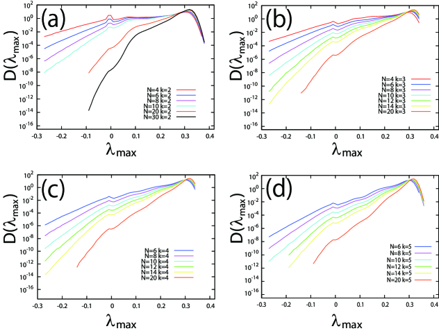
Figure 1:

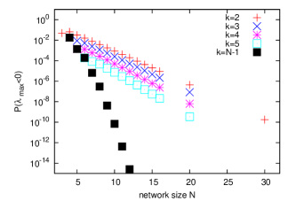
Figure 2:

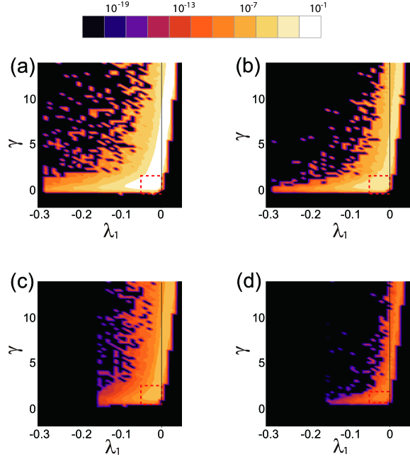
Figure 3:

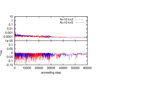
Figure 4:

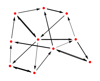
Figure 5:

References

- [1] J. Visser, J. Hermisson, G.P. Wagner, L.A. Meyers, H. Bagheri-Chaichian, J.L. Blanchard, L. Chao, J.M. Cheverud, S.F. Elena, W. Fontana, et al. Perspective: evolution and detection of genetic robustness. Evolution, 57(9):1959–1972, 2003.
- [2] F. Li, T. Long, Y. Lu, Q. Ouyang, and C. Tang. The yeast cell-cycle network is robustly designed. Proceedings of the National Academy of Sciences of the United States of America, 101(14):4781, 2004.
- [3] A. Wagner. Robustness and evolvability in living systems. Princeton University Press Princeton, NJ:, 2005.
- [4] J. Masel and M.V. Trotter. Robustness and Evolvability. Trends in Genetics, 2010.
- [5] S.A. Kauffman. The origins of order: Self organization and selection in evolution. Oxford University Press, USA, 1993.
- [6] K. Kaneko. Clustering, coding, switching, hierarchical ordering, and control in a network of chaotic elements. Physica D: Nonlinear Phenomena, 41(2):137–172, 1990.
- [7] B. A. Berg and T. Neuhaus. Multicanonical algorithms for first order phase transitions. Phys. Lett. B, 267(2):249–253, 1991.
- [8] B. A. Berg and T. Celik. New approach to spin-glass simulations. Phys. Rev. Lett., 69(15):2292–2295, 1992.
- [9] E. Ott. Chaos in dynamical systems. Cambridge Univ Pr, 2002.
- [10] B. A. Berg and T. Neuhaus. Multicanonical ensemble: A new approach to simulate first-order phase transitions. Phys. Rev. Lett., 68(1):9–12, 1992.
- [11] Yukito Iba. Extended ensemble monte carlo. International Journal of Modern Physics C, 12(05):623–656, 2001.
- [12] F. Wang and D. P. Landau. Efficient, multiple-range random walk algorithm to calculate the density of states. Phys. Rev. Lett., 86(10):2050–2053, 2001.
- [13] F. Wang and D. P. Landau. Determining the density of states for classical statistical models: A random walk algorithm to produce a flat histogram. Phys. Rev. E, 64(5):056101, 2001.
- [14] Nen Saito and Yukito Iba. Probability of graphs with large spectral gap by multicanonical monte carlo. Computer Physics Communications, 182(1):223–225, 2011.
- [15] N. Saito, Y. Iba, and K. Hukushima. Multicanonical sampling of rare events in random matrices. Physical Review E, 82(3):031142, 2010.
- [16] A. Varma, M. Morbidelli, and H. Wu. Parametric sensitivity in chemical systems. Cambridge Univ Pr, 1999.
- [17] T.M. Perumal, Y. Wu, and R. Gunawan. Dynamical analysis of cellular networks based on the Green’s function matrix. Journal of theoretical biology, 261(2):248–259, 2009.
- [18] S. Bornholdt and K. Sneppen. Robustness as an evolutionary principle. Proceedings of the Royal Society B: Biological Sciences, 267(1459):2281, 2000.
- [19] A. Szejka and B. Drossel. Evolution of canalizing Boolean networks. The European Physical Journal B-Condensed Matter and Complex Systems, 56(4):373–380, 2007.
- [20] V. Sevim and P.A. Rikvold. Chaotic gene regulatory networks can be robust against mutations and noise. Journal of theoretical biology, 253(2):323–332, 2008.
- [21] Christian Torres-Sosa, Sui Huang, and Maximino Aldana. Criticality is an emergent property of genetic networks that exhibit evolvability. PLoS Computational Biology, 8(9):e1002669, 2012.
- [22] R. Serra, M. Villani, A. Graudenzi, and SA Kauffman. Why a simple model of genetic regulatory networks describes the distribution of avalanches in gene expression data. Journal of theoretical biology, 246(3):449–460, 2007.
- [23] I. Shmulevich, S.A. Kauffman, and M. Aldana. Eukaryotic cells are dynamically ordered or critical but not chaotic. Proceedings of the National Academy of Sciences of the United States of America, 102(38):13439, 2005.
- [24] M. Nykter, N.D. Price, M. Aldana, S.A. Ramsey, S.A. Kauffman, L.E. Hood, O. Yli-Harja, and I. Shmulevich. Gene expression dynamics in the macrophage exhibit criticality. Proceedings of the National Academy of Sciences, 105(6):1897, 2008.
- [25] E. Balleza, E.R. Alvarez-Buylla, A. Chaos, S. Kauffman, I. Shmulevich, and M. Aldana. Critical dynamics in genetic regulatory networks: examples from four kingdoms. PLoS One, 3(6):e2456, 2008.
- [26] S. Chowdhury, J. Lloyd-Price, O.P. Smolander, W.C.V. Baici, T.R. Hughes, O. Yli-Harja, G. Chua, and A.S. Ribeiro. Information propagation within the genetic network of saccharomyces cerevisiae. BMC Systems Biology, 4(1):143, 2010.
- [27] John M Beggs and Dietmar Plenz. Neuronal avalanches in neocortical circuits. The Journal of neuroscience, 23(35):11167–11177, 2003.
- [28] John M Beggs and Dietmar Plenz. Neuronal avalanches are diverse and precise activity patterns that are stable for many hours in cortical slice cultures. The Journal of neuroscience, 24(22):5216–5229, 2004.
- [29] Dietmar Plenz, Tara C Thiagarajan, et al. The organizing principles of neuronal avalanches: cell assemblies in the cortex? Trends in neurosciences, 30(3):101, 2007.
- [30] N. Metropolis, A. W. Rosenbluth, M. N. Rosenbluth, A. H. Teller, and E. Teller. Equation of State Calculations by Fast Computing Machines. J. Chem. Phys., 21(6):1087, 1953.
- [31] W. K. Hastings. Monte Carlo sampling methods using Markov chains and their applications. Biometrika, 57:97–109, 1970.