Dynamical apparent horizons in inhomogeneous Brans–Dicke universes

Abstract

The presence and evolution of apparent horizons in a two-parameter family of spherically symmetric, time-dependent solutions of Brans–Dicke gravity are analyzed. These solutions were introduced to model space- and time-varying gravitational couplings and are supposed to represent central objects embedded in a spatially flat universe. We find that the solutions possess multiple evolving apparent horizons, both black hole horizons covering a central singularity and cosmological ones. It is not uncommon for two of these horizons to merge, leaving behind a naked singularity covered only by a cosmological horizon. Two characteristic limits are also explicitly worked out: the limit where the theory reduces to general relativity and the limit where the solutions become static. The physical relevance of this family of solutions is discussed.

I Introduction

Varying “constants” of nature, first hypothesized by Dirac Dirac , can be implemented naturally in the context of scalar-tensor gravity, in which the gravitational coupling becomes a function of the spacetime point BransDicke61 ; ST . String theories GreenSchwarzWitten contain a dilaton field coupling non-minimally to gravity which mimics a Brans–Dicke-like scalar field (indeed, it is well known that the low-energy limit of the bosonic string theory is an $\omega_{0}=-1$ Brans–Dicke theory bosonic ). Scalar-tensor cosmology, in which the effective gravitational coupling $G_{\rm eff}$ depends on time, has been the subject of much work FujiiMaeda03 ; mybook but much less attention has been devoted to inhomogeneous solutions in which $G_{\rm eff}$ depends also on space. However, there is really no support for assuming that this spatial dependence can be neglected BarrowOToole01 ; CliftonMotaBarrow05 . Spherically symmetric inhomogeneous solutions of scalar-tensor gravity representing a central condensation embedded in a cosmological background have been found in CliftonMotaBarrow05 .

There is plenty of additional motivation for studying analytical solutions of gravitational theories representing a central object in a cosmological space. First, the present acceleration of the cosmic expansion SN requires, if one is to remain within the boundaries of general relativity, that approximately 73% of the energy content of the universe is in the form of exotic (pressure $P^{(m)}\sim-\rho^{(m)}$) dark energy Komatsu (see LinderResourceLetter for a list of references and AmendolaTsujikawabook for a comprehensive discussion). An alternative to this ad hoc explanation is that gravity deviates from general relativity at large scales. Further motivation for alternative gravity comes from the fact that virtually all theories attempting to quantize gravity produce, in the low-energy limit, not general relativity but modifications of it containing corrections such as non-minimally coupled dilatons and/or higher derivative terms.

These ideas have led to the introduction (or better, revival) of $f(R)$ gravity to replace Einstein theory at large scales CCT ; CDDT ; Vollick ; metricaffine and explain the cosmic acceleration (see review ; DeFeliceTsujikawa for reviews and otherreviews for shorter introductions). Since the $f(R)$ theories of interest for cosmology are designed to produce a time-varying effective cosmological “constant”, spherically symmetric solutions representing black holes or central condensations in these theories are expected to be asymptotically Friedmann-Lemaître-Robertson-Walker (FLRW), not asymptotically flat, and to be dynamical. Very few such solutions are known, among them the inhomogeneous time-dependent solution of Clifton in $f(R)=R^{1+\delta}$ gravity Clifton ; myClifton .

Second, analytical solutions describing central objects in a cosmological background are of interest also in general relativity. The first study of this kind of solution by McVittie McVittie is related to investigations of the problem of whether, and to what extent, the cosmic expansion affects local systems (see CarreraGiulini for a recent review). In addition to the old (and largely overlooked) McVittie solution McVittie , which is not yet completely understood Klebanetal ; LakeAbdelqader ; Roshina ; FZN relatively few other solutions with similar features have been reported over the years cosmologicalblackholes .

Third, more recent interest in cosmological condensations in the context of general relativity arises from yet another attempt to explain the present cosmic acceleration without dark energy and without modifying gravity. This is the idea that the backreaction of inhomogeneities on the cosmic dynamics is sufficient to produce the observed acceleration backreaction . However, the formalism implementing this idea is plagued by formal problems and it has not been shown to be able to explain convincingly the cosmic acceleration. Indeed, even the sign of the backreaction terms in the equation giving the averaged acceleration has not been shown to be the correct one thatreview ; Larenagauge ; VitaglianoLiberatiFaraoni09 and recent work casts even more serious doubts on this proposed solution to the cosmic acceleration problem GreenWald .

Attempts to move beyond these riddles involve the consideration of analytical solutions of Einstein theory describing cosmological inhomogeneities and including Lemaître-Tolman-Bondi, Swiss-cheese, and other models backreactionexact ; Krasinskibook . Moreover, the teleological nature of the event horizon has prompted the consideration of apparent, trapping, isolated, dynamical, and slowly evolving horizons (dynamicalhorizons ; Nielsenreview and references therein), a subject of great interest dynamicalBHthermo . There has also been interest in dynamical black hole horizons in relation to the accretion of dark energy accretion . Physically, black hole event horizons can only be traversed from the outside to the inside while, for the traditional cosmological event and particle horizons, signals can cross from the inside to the outside but not vice-versa. Event horizons are null surfaces and are appropriate to describe stationary situations but, as said, they require the knowledge of the entire spacetime manifold to even be defined. An apparent horizon is a spacelike or timelike surface defined as the closure of a 3-surface which is foliated by marginal surfaces (those on which the expansion of the congruence of radial null geodesics vanishes) HaywardPRD49 .

With all these motivations in mind, it is interesting to further explore analytical solutions of alternative gravity theories representing spherical objects in cosmological backgrounds. Here we consider the class of solutions discovered by Clifton, Mota, and Barrow CliftonMotaBarrow05 in Brans–Dicke theory, described by the action BransDicke61

$$S_{BD}=\int d^{4}x\,\sqrt{-g}\left[\phi R-\frac{\omega_{0}}{\phi}\,g^{\mu\nu}\nabla_{\mu}\phi\nabla_{\nu}\phi+2\kappa\,{\cal L}^{(m)}\right]\,,$$ (1)

where $\kappa\equiv 8\pi G$, $G$ is Newton’s constant, ${\cal L}^{(m)}$ is the matter Lagrangian, and the Brans–Dicke scalar field $\phi$ corresponds to the inverse of the gravitational coupling $G_{\rm eff}$. Matter is assumed to be a perfect fluid with energy density $\rho^{(m)}$, pressure $P^{(m)}$, and equation of state $P^{(m)}=\left(\gamma-1\right)\rho^{(m)}$, where $\gamma$ is a constant CliftonMotaBarrow05 . In the following sections we analyze and discuss the structure of the solutions of CliftonMotaBarrow05 , focussing on the dynamical behaviour of their apparent horizons, in an attempt to understand if the these solution harbor black holes or naked singularities. The bizarre behaviour of the apparent horizons we find seems to be rather typical of solutions describing cosmological black holes HusainMartinezNunez in a certain region of the parameter space, but other behaviours appear for different combinations of the parameters.

Note that, even though it is standard procedure to rely on apparent horizons as proxies for event horizons to characterize black holes in theoretical and numerical relativity Nielsenreview ; proxies , it is also well known that apparent horizons depend on the spacetime slicing adopted foliationdependence (this problem is perhaps less worrisome when spherical symmetry is assumed). We adopt the same practice here, bearing the caveat just mentioned in mind.

II Clifton-Mota-Barrow solutions

We begin with the Clifton-Mota-Barrow spherically symmetric and time-dependent metric CliftonMotaBarrow05

$$ds^{2}=-e^{\nu(\varrho)}dt^{2}+a^{2}(t)e^{\mu(\varrho)}(d\varrho^{2}+\varrho^{2}d\Omega^{2})\,,$$ (2)

where $d\Omega^{2}=d\theta^{2}+\sin^{2}\theta\,d\varphi^{2}$ denotes the line element on the unit 2-sphere,

$$e^{\nu(\varrho)} = \left(\frac{1-\frac{m}{2\alpha\varrho}}{1+\frac{m}{2\alpha\varrho}}\right)^{2\alpha}\equiv A^{2\alpha}\,,$$ (3)

$$e^{\mu(\varrho)} = \left(1+\frac{m}{2\alpha\varrho}\right)^{4}A^{\frac{2}{\alpha}(\alpha-1)(\alpha+2)}\,,$$ (4)

$$a(t) = a_{0}\left(\frac{t}{t_{0}}\right)^{\frac{2\omega_{0}(2-\gamma)+2}{3\omega_{0}\gamma(2-\gamma)+4}}\equiv a_{\ast}t^{\beta}\,,$$ (5)

$$\phi(t,\varrho) = \phi_{0}\left(\frac{t}{t_{0}}\right)^{\frac{2(4-3\gamma)}{3\omega_{0}\gamma(2-\gamma)+4}}A^{-\frac{2}{\alpha}(\alpha^{2}-1)}\,,$$ (6)

$$\alpha = \sqrt{\frac{2(\omega_{0}+2)}{2\omega_{0}+3}}\,,$$ (7)

$$\rho^{(m)}(t,\varrho) = \rho_{0}^{(m)}\left(\frac{a_{0}}{a(t)}\right)^{3\gamma}A^{-2\alpha}\,,$$ (8)

$\rho^{(m)}$ is the energy density of the cosmic fluid, $\omega_{0}$ is the Brans–Dicke parameter, $m$ is a mass parameter, $\alpha,\phi_{0},a_{0}$, $\rho^{(m)}_{0}$ and $t_{0}$ are positive constants (where $\phi_{0}$, $\rho^{(m)}_{0}$ and $t_{0}$ are not actually fully independent). Moreover, $\varrho$ is the isotropic radius related to the Schwarzschild radial coordinate $\tilde{r}$ by

$$\tilde{r}\equiv\varrho\left(1+\frac{m}{2\alpha\varrho}\right)^{2}\,,$$ (9)

so that

$$d\tilde{r}=\left(1-\frac{m^{2}}{4\alpha^{2}\varrho^{2}}\right)d\varrho\,.$$ (10)

The quantity $\alpha$ is real for $\omega_{0}<-2$ and for $\omega_{0}>-3/2$. For definiteness, we impose that $\omega_{0}>-3/2$ and $\beta\geq 0$. The Clifton-Mota-Barrow metric (2) is separable and reduces to the spatially flat Friedmann–Lemaître–Robertson–Walker (FLRW) metric in the limit $m\rightarrow 0$ in which the central mass disappears. For $\gamma\neq 2$, setting $\omega_{0}=\left(\gamma-2\right)^{-1}$ yields $\beta=0$ and the metric becomes static, whereas the scalar field remains time-dependent. Setting $\gamma=2$ or $\gamma=4/3$ leads to $\beta=1/2$ and the scale factor scales as $\sqrt{t}$ independent of the value of the Brans–Dicke coupling $\omega_{0}$. We will consider the physically interesting special cases in a separate section below.

Our main concern here is whether the solutions in the Clifton–Mota–Barrow class represent black holes or naked singularities, embedded in a cosmological background (by naked singularity we simply mean a timelike or null singularity which is not covered by an event horizon). To answer this question, we would like to determine the location and the nature of horizons. Since the spacetime is dynamical, it is appropriate to consider apparent, instead of event, horizons and, therefore, we will locate the apparent horizons and study their dynamics.

III Finding the apparent horizons

We proceed by rewriting the metric in the more familiar form

$$ds^{2}=-A^{2\alpha}dt^{2}+a^{2}(t)A^{\frac{2}{\alpha}(\alpha^{2}-2)}d\tilde{r}^{2}+r^{2}d\Omega^{2}\,,$$ (11)

using the areal radius

$$r = a(t)\varrho\left(1+\frac{m}{2\alpha\varrho}\right)^{2}A^{\frac{1}{\alpha}(\alpha-1)(\alpha+2)}$$ (12)

$$= a(t)\tilde{r}A^{\frac{1}{\alpha}(\alpha-1)(\alpha+2)}\,.$$

The differential $dr$ is related to $d\tilde{r}$ by

$$dr = \dot{a}(t)\,\tilde{r}A^{\frac{1}{\alpha}(\alpha-1)(\alpha+2)}dt+a(t)A^{\frac{1}{\alpha}(\alpha-1)(\alpha+2)}d\tilde{r}$$ (13)

$$+\frac{a(t)m}{\alpha^{2}\tilde{r}}(\alpha-1)(\alpha+2)A^{\frac{1}{\alpha}(\alpha-1)(\alpha+2)-2}d\tilde{r}\,,\,\,\,$$

which means that

$$d\tilde{r}=\frac{dr-\dot{a}(t)\tilde{r}A^{\frac{1}{\alpha}(\alpha-1)(\alpha+2)}dt}{a(t)A^{\frac{1}{\alpha}(\alpha-1)(\alpha+2)-2}\left[A^{2}+\frac{m}{\alpha^{2}\tilde{r}}(\alpha-1)(\alpha+2)\right]}\,.$$ (14)

The line element can now be written as

$$ds^{2} = -\left[A^{2\alpha}-\frac{\dot{a}^{2}(t)\tilde{r}^{2}}{B^{2}(\varrho)}A^{\frac{2}{\alpha}(\alpha^{2}+2\alpha-2)}\right]dt^{2}$$ (15)

$$-2\,\frac{\dot{a}(t)\tilde{r}}{B^{2}(\varrho)}A^{\frac{\alpha^{2}+3\alpha-2}{\alpha}}drdt$$

$$+\frac{A^{2}(\varrho)}{B^{2}(\varrho)}dr^{2}+r^{2}d\Omega^{2}\,,$$

where we have defined the positive function

$$B(\varrho)\equiv A^{2}(\varrho)+\frac{(\alpha-1)(\alpha+2)}{\alpha^{2}}\,\frac{m}{\tilde{r}}\,.$$ (16)

(Note that $B>0$ is a consequence of $\alpha=\sqrt{\frac{2(\omega_{0}+2)}{2\omega_{0}+3}}\geq 1$.)

We now introduce a new time coordinate $\bar{t}$ which serves the purpose of eliminating the time-radius cross term. Define $\bar{t}$ such that

$$d\bar{t}=\frac{1}{F(t,r)}\left[dt+\psi(t,r)dr\right]\,,$$ (17)

where $\psi(t,r)$ is a function to be fixed later and $F(t,r)$ is an integrating factor which guarantees that $d\bar{t}$ is an exact differential and satisfying the equation

$$\frac{\partial}{\partial r}\left(\frac{1}{F}\right)=\frac{\partial}{\partial t}\left(\frac{\psi}{F}\right)\,.$$ (18)

The line element then assumes the form

$$ds^{2} = -\left[A^{2\alpha}-\frac{\dot{a}^{2}(t)\tilde{r}^{2}}{B(\varrho)^{2}}A^{\frac{2}{\alpha}(\alpha^{2}+2\alpha-2)}\right]F^{2}d\bar{t}^{2}+\left\{2\psi F\left[A^{2\alpha}-\frac{\dot{a}^{2}(t)\tilde{r}^{2}}{B(\varrho)^{2}}A^{\frac{2}{\alpha}(\alpha^{2}+2\alpha-2)}\right]-2\,\frac{F\dot{a}(t)\tilde{r}}{B(\varrho)^{2}}A^{\frac{\alpha^{2}+3\alpha-2}{\alpha}}\right\}drd\bar{t}$$ (19)

$$+\left\{\frac{A^{2}}{B(\varrho)^{2}}-\psi^{2}\left[A^{2\alpha}-\frac{\dot{a}^{2}(t)\tilde{r}^{2}}{B(\varrho)^{2}}A^{\frac{2}{\alpha}(\alpha^{2}+2\alpha-2)}\right]+2\,\frac{\psi\dot{a}(t)\tilde{r}}{B(\varrho)^{2}}A^{\frac{\alpha^{2}+3\alpha-2}{\alpha}}\right\}dr^{2}+r^{2}d\Omega^{2}\,.$$

The choice

$$\psi=\frac{\dot{a}(t)\tilde{r}}{B^{2}}\frac{A^{\frac{-\alpha^{2}+3\alpha-2}{\alpha}}}{D(t,\varrho)}$$ (20)

for the function $\psi$, with

$$D(t,\varrho)\equiv 1-\frac{\dot{a}^{2}(t)\tilde{r}^{2}}{B^{2}}A^{\frac{4}{\alpha}(\alpha-1)}\,,$$ (21)

turns the metric into the simple form

$$ds^{2} = -A^{2\alpha}DF^{2}d\bar{t}^{2}+\left(\frac{H^{2}}{B^{4}D}r^{2}A^{2(2-\alpha)}+\frac{A^{2}}{B^{2}}\right)dr^{2}$$ (22)

$$+r^{2}d\Omega^{2}\,,$$

where $H\equiv\dot{a}(t)/a(t)$ denotes the Hubble parameter of the background FLRW universe. We are now able to locate the apparent horizons (when they exist), which are the loci of spacetime points satisfying $\nabla^{c}r\nabla_{c}r=0$, or $g^{rr}=0$ NielsenVisser ; Nielsenreview , that is

$$\frac{B^{4}D}{H^{2}r^{2}A^{2(2-\alpha)}+A^{2}B^{2}D}=0\,.$$ (23)

The solution of this equation reduces to the condition $D=0$, or

$$B^{2}A^{2(\alpha-1)}=H^{2}r^{2}\,,$$ (24)

which, explicitly, reads

$$A^{\alpha-1}\!\left[A^{2}\!+\frac{(\alpha-1)(\alpha+2)}{\alpha^{2}}\,\frac{ma(t)}{r}\,A^{\frac{(\alpha-1)(\alpha+2)}{\alpha}}\right]\!=\pm Hr\,.$$ (25)

In an expanding universe with $H>0$ the quantity in square brackets is positive, hence we choose the positive sign. Eq. (25) can then be written as

$$Hr^{2}-\frac{(\alpha-1)(\alpha+2)}{\alpha^{2}}\,m\,a(t)A^{\frac{2(\alpha-1)(\alpha+1)}{\alpha}}-A^{\alpha+1}r=0\,.$$ (26)

The Ricci scalar becomes singular as $r\rightarrow 0$ for all positive values of the mass parameter $m$ (see Appendix A) and this limit denotes a central singularity. The energy density (8) of the cosmic fluid also diverges in this limit.

IV Special cases and limits

Before determining the generic behaviour of apparent horizons, it is useful to look into some special limits, of either the theory or the solutions, which will help us gain some intuition.

IV.1 The zero mass limit

In the limit $m\rightarrow 0$ in which there is no central object, eq. (26) reduces to $Hr^{2}=r$, which yields $r=H^{-1}$, the Hubble horizon. This value is also obtained in the limit of large $\varrho$ in which $r$ becomes a comoving radius and the metric approaches the spatially flat FLRW metric. This is best seen using eq. (24) as at this limit $A,B\to 1$ (the limit is less straightforward in eq. (26) as $r\to\infty$ and $\varrho\to\infty$). Therefore, we expect the horizon at larger radii to be a cosmological one.

IV.2 The static limit

We now consider the limit in which the metric becomes static, which corresponds to $\beta=0$ and yields $a(t)\equiv a_{0}$, see eq. (5). This value for $\beta$ is obtained for $\omega_{0}=\left(\gamma-2\right)^{-1}$ (with $\gamma\neq 2$). This requirement implies that for each theory in the Brans–Dicke class, (i.e., for each value of $\omega_{0}$) there is at most one solution with a static metric in the Clifton–Mota–Barrow family, and it corresponds to a specific choice of equation of state for the fluid. As mentioned earlier, for $\alpha$ to be real, one needs to have $\omega_{0}<-2$ or $\omega_{0}>-3/2$. This translates to $\gamma>3/2$ or $\gamma<4/3$ when the $\beta=0$ condition has been imposed.

Eqs. (6) and (8) yield

$$\phi(t,r) = \phi_{0}\left(\frac{t}{t_{0}}\right)^{2}A^{-\frac{2(\alpha^{2}-1)}{\alpha}}\,,$$ (27)

$$\rho^{(m)} = \rho_{0}^{(m)}A^{-2\alpha}\,.$$ (28)

The Brans–Dicke field $\phi$ depends on time even though the metric $g_{\mu\nu}$ and the matter energy density $\rho^{(m)}$ do not. In fact, there is no solution in the Clifton–Mota–Barrow class which is genuinely static.

In terms of the areal radius $r$, it is

$$ds^{2}=-A^{2\alpha}dt^{2}+\frac{A^{2}}{B^{2}}dr^{2}+r^{2}d\Omega^{2}\,,$$ (29)

and the apparent horizons are located by the equation $g^{rr}=0$ equivalent to $B=0$, or

$$\varrho^{2}+\frac{m}{\alpha^{2}}\left(\alpha^{2}-2\right)\varrho+\frac{m^{2}}{4\alpha^{2}}=0\,.$$ (30)

The discriminant of this quadratic equation is $\Delta(\alpha^{2})=\frac{m^{2}}{\alpha^{2}}\left[\left(\alpha^{2}-2\right)^{2}-\alpha^{2}\right]$ and one easily finds that $\Delta\geq 0$ for $\alpha\leq 1$ and $\alpha\geq 2$ (remember that $\alpha\geq 0$, cf. eq. (7)). Therefore, for $1<\alpha<2$ there are no real roots and no apparent horizons. For $\alpha\leq 1$ and for $\alpha\geq 2$ the real roots,

$$\varrho_{\pm}=\frac{m}{\alpha^{2}}\left[-\left(\alpha^{2}-2\right)\pm\sqrt{\left(\alpha^{2}-2\right)^{2}-\alpha^{2}}\right]\,,$$ (31)

are both negative and do not correspond to apparent horizons. We conclude that the solution with static metric always describes a naked singularity.

IV.3 The limit to general relativity

We now consider the limit to general relativity obtained for $\omega_{0}\rightarrow\infty$. When $\gamma\neq 0$ and $\gamma\neq 2$, this limit yields $\alpha\rightarrow 1$, $\phi\rightarrow\phi_{0}$, and

$$ds^{2} = -\left(\frac{1-\frac{m}{2\varrho}}{1+\frac{m}{2\varrho}}\right)^{2}dt^{2}+a^{2}(t)\left(1+\frac{m}{2\varrho}\right)^{4}\cdot$$ (32)

$$\cdot\left(d\varrho^{2}+\varrho^{2}d\Omega^{2}\right)\,,$$

$$a(t) = a_{0}\left(\frac{t}{t_{0}}\right)^{\frac{2}{3\gamma}}\,,$$ (33)

$$\rho^{(m)}(t) = \rho_{0}^{(m)}\left(\frac{t_{0}}{t}\right)^{2}A^{-2}\,.$$ (34)

This metric corresponds to one of the generalized McVittie metrics studied in Refs. generalizedMcVittie ; generalizedMcVittie2 ; McVittieattractor which, in isotropic coordinates, assume the form

$$ds^{2} = -\left(\frac{1-\frac{M(t)}{2\varrho a(t)}}{1+\frac{M(t)}{2\varrho a(t)}}\right)^{2}dt^{2}$$ (35)

$$+a^{2}(t)\left(1+\frac{M(t)}{2\varrho a(t)}\right)^{4}\left(d\varrho^{2}+\varrho^{2}d\Omega^{2}\right)\,,$$

where $M(t)$ is an arbitrary positive regular function of time.

The McVittie solution of general relativity originally introduced to study the effect of the cosmological expansion on local systems McVittie is obtained for $M(t)=$ const. This time independence of the function $M(t)$ in this case follows from the McVittie condition $G^{1}_{0}=0$ which corresponds to zero radial energy flow $T_{0}^{1}=0$. Lifting this restriction and allowing for radial accretion of energy generates the solutions (35) with general functions $M(t)$ (see the discussion in Ref. generalizedMcVittie ). It is shown in Ref. McVittieattractor that, in the class of generalized McVittie solutions (35), the solution with “comoving mass function” $M(t)=M_{0}a(t)$ (where $M_{0}$ is a constant) is a late-time attractor for solutions characterized by a background universe which keeps expanding in the future ($a\rightarrow+\infty$). This is precisely the $\omega_{0}\rightarrow\infty$ limit of the scalar-tensor solution (2)-(8), which also makes it clear that the Clifton–Mota–Barrow solutions are indeed accreting. Incidentally, the generalized McVittie solutions (35) of general relativity were derived two years after the discovery of the Clifton-Mota-Barrow solution (2)-(8) and the one with late-time attractor behaviour and with $M=M_{0}\,a(t)$ could, in principle, have been discovered by taking the limit to general relativity of this Brans–Dicke solution.

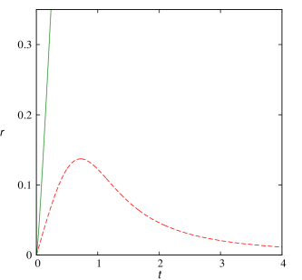
Figure 1: Radii of the apparent horizons in units of $(ma_{*})^{1/(1-\beta)}$ as functions of time in the same units for $\omega_{0}=-17/12$. The red, dashed curve corresponds to dust ($\gamma=1$) and the green, solid curve corresponds to both radiation ($\gamma=4/3$) and stiff matter ($\gamma=2$). For dust, there is only one apparent horizon whose radius reaches a maximum and then decreases. For radiation and stiff matter, instead, there is a naked singularity in a universe which expands forever.

The apparent horizons of the generalized McVittie metrics (35) have been discussed in generalizedMcVittie2 . For large values of $\omega_{0}$, the solution (2)-(8) approaches the attractor McVittie solution and its apparent horizons should also approach those of the attractor McVittie metric: jumping ahead slightly, this is indeed the case, as can be seen by comparing our Fig. 4 with Fig. 3 of Ref. generalizedMcVittie2 .

The $\gamma=0$ case, which corresponds to a cosmological constant, leads to a diverging exponent $\beta$ for the scale factor $a(t)$ when $\omega_{0}\to\infty$. This behaviour can be attributed to the fact that the Clifton–Mota–Barrow solution assumes a power law form for the scale factor, whereas the general relativity limit of the solution is actually expected to be Schwarzschild–de Sitter spacetime.

For $\gamma=2$ the $\omega_{0}\to\infty$ limit yields $\alpha\to 1$, $\phi\propto t^{-1}$, $a(t)\propto\sqrt{t}$, $\rho^{(m)}(t)\propto t^{-3}A^{-2}$, and the metric is the same as in eq. (32).

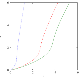
Figure 2: Same as Fig. 1 but for $\omega_{0}=-1/3$. The blue, dotted line corresponds to a cosmological constant ($\gamma=0$). In all cases there is one, ever expanding horizon, and so the solution appears to represents a naked singularity in an expanding universe.

V Generic behaviour of apparent horizons

Having discussed the special cases, we now turn our attention to the behaviour of apparent horizons in generic solutions of the Clifton–Mota–Barrow family. In order to solve eq. (26) and determine the location of these horizons, it is convenient to introduce the new quantity $x\equiv\frac{m}{2\alpha\varrho}$, in terms of which it is

$$A=\frac{1-x}{1+x}\,,$$ (36)

while $H=\beta/t$. One can now express parametrically the radius $r$ of the apparent horizon(s) and the time coordinate as functions of the parameter $x$, obtaining

$$r(x) = a_{\ast}t^{\beta}\frac{m}{2\alpha}\,\frac{(1+x)^{2}}{x}\left(\frac{1-x}{1+x}\right)^{\frac{(\alpha-1)(\alpha+2)}{\alpha}}\,,$$ (37)

$$t(x) = \left\{\frac{2\alpha}{m\,a_{\ast}\beta}\,\frac{x}{(1+x)^{\frac{2}{\alpha}(\alpha+1)}}\left[(1-x)^{2/\alpha}\right.\right.$$

$$+ \left.\left.2x\,\frac{(\alpha-1)(\alpha+2)}{\alpha}\,(1-x)^{-2(\alpha-1)/\alpha}\right]\right\}^{\frac{1}{\beta-1}}\,.$$

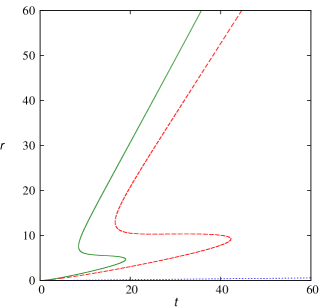
(a)  $\omega_{0}=1$

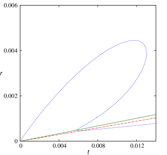
(b)  $\omega_{0}=1$, zoom-in

Figure 3: Same as previously but for $\omega_{0}=1$. For all three values of $\gamma$, at early times there is only one horizon. As the universe expands, the singularity gets covered by two more apparent horizons. Two of the horizons eventually merge and disappear, leaving behind only the cosmological horizon covering a naked singularity.

The radii of the apparent horizons as functions of time are plotted in Figs. 1 to 4 for the values of the Brans–Dicke parameter $\omega_{0}=-17/12$, $-1/3$, $1$, and $10^{5}$, respectively, and for various choices of the equation of state parameter $\gamma$. In these plots $r$ and $t$ are actually measured in units of

$$(ma_{*})^{\frac{1}{1-\beta}}=\left(a_{0}\,\frac{m}{t_{0}}\right)^{\frac{1}{1-\beta}}t_{0}\,,$$ (39)

as this convenient normalization completely absorbs the dependence on the parameters $m$, $a_{0}$, $t_{0}$.

The blue, dotted curves correspond to a cosmological constant ($\gamma=0$) and the red, dashed curves correspond to dust ($\gamma=1$). The green, solid curves show the behaviour of the apparent horizons for both radiation ($\gamma=4/3$) and stiff matter ($\gamma=2$). This is because $\beta$, which determines the scaling of the scale factor with time, is equal to $1/2$ and independent of $\omega_{0}$ for both of these values. For $\omega_{0}=-17/12$ (Fig. 1) we do not consider the case of a cosmological constant, corresponding to $\gamma=0$, as it leads to a contracting universe.

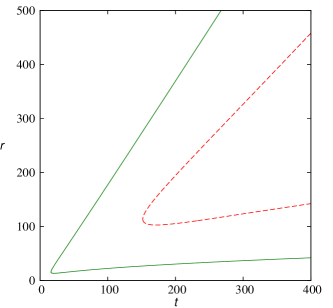
(a)  $\omega_{0}=10^{5}$

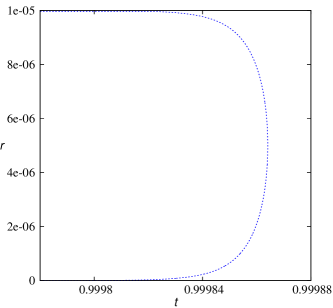
(b)  $\omega_{0}=10^{5}$, zoom-in

Figure 4: Same as previously but for $\omega_{0}=10^{5}$, $\omega_{0}\to\infty$ being the limit to general relativity. Here for all three cases there are two horizons, presumably a black hole horizon and a cosmological horizon. For a cosmological constant (blue, dotted curve) these two horizon merge and disappear. For the other two cases, there is initially a naked singularity which eventually gets covered by the two horizons.

As can be seen in the figures (see captions for more details), for $\omega_{0}=-17/12$ and $\omega_{0}=-1/3$ there is only one apparent horizon for all of the values of $\gamma$ we have considered. In most cases, this horizon is expanding forever, so the solution is most likely to represent a naked singularity in an expanding universe. For $\omega_{0}=-17/12$ and for dust ($\gamma=1$), on the other hand, the apparent horizon exhibits a perhaps more remarkable behaviour: it initially expands, to reach a maximum radius and then contracts to reach zero radius asymptotically.

Even more noteworthy is the behaviour of the apparent horizons when $\omega_{0}=1$ (Fig. 3). For dust, radiation, and stiff matter there is initially one expanding apparent horizon, see Fig. 3(a). Two more apparent horizons appear. The outer one expands, while the inner one eventually merges with the initial one and they both disappear. Similar phenomenology was reported in Ref. myClifton for Clifton’s solution Clifton of metric $f(R)=R^{1+\delta}$ gravity.

In fact, this puzzling behaviour was found long ago in the Husain-Martinez-Nuñez solution HusainMartinezNunez describing a black hole embedded in a universe filled with a free massless scalar field minimally coupled to gravity and accreting onto the black hole (compare Fig. 3(a) with Fig. 1 of Ref. HusainMartinezNunez ).

For $\omega_{0}=1$ and $\gamma=0$, which corresponds to a cosmological constant and is presented in Fig. 3(b), the situation is similar, except for the fact that the pair of horizons actually appears inside the initial horizon. Such behaviour has not been reported before to the best of our knowledge.

Finally, Fig. 4 corresponds to the large value of the Brans–Dicke parameter $\omega_{0}=10^{5}$. The behaviour of the apparent horizon dynamics is very similar to that present in the general relativity limit of the Clifton-Mota-Barrow solution obtained for $\omega_{0}\rightarrow\infty$ and discussed in Sec. IV.3. For dust, radiation and stiff matter, the singularity is initially naked and eventually gets covered by two expanding horizons, see Fig. 4(a). For a cosmological constant this picture is reversed: there are initially two nested horizons, one expanding and one contracting, which eventually merge and disappear, leaving the singularity naked, see Fig. 4(b).

VI Discussion and conclusions

There are relatively few solutions describing central matter configurations embedded in FLRW backgrounds in general relativity, and even fewer in alternative theories of gravity. We have studied here the Clifton–Mota–Barrow class of spacetimes, which are solutions of Brans–Dicke theory. The latter is perhaps the minimal implementation of a varying gravitational coupling, containing only a scalar extra degree of freedom. As such, it is justly regarded as the prototypical alternative to Einstein’s theory. It is, therefore, quite interesting to assess whether or under which conditions can the Clifton–Mota–Barrow spacetimes describe a realistic localized matter configuration embedded in an evolving universe.

Given that these spacetimes contain singularities, we have focussed our study on the behaviour of dynamical apparent horizons. According to the position in parameter space, we have uncovered different types of behaviour for these horizons. The most important result is perhaps that, for certain values of the parameters, the Clifton–Mota–Barrow spacetime appears to contain a naked singularity (at least as far as one can tell based on the presence/absence of apparent horizons; though unlikely, it is possible that the particular slicing of the spacetime leads to the absence of an apparent horizon even though the singularity is cloaked by an event horizon). In some cases, this singularity is present from the time of the big bang, thus preventing us from obtaining the metric and scalar field as regular developments of Cauchy data, and later gets covered by black hole and cosmological horizons. For other values of the parameters, pairs of black hole and cosmological horizons appear and bifurcate, or merge and disappear, a phenomenology known from a solution of general relativity HusainMartinezNunez and one of $f(R)$ gravity Clifton ; myClifton . Overall, the Clifton–Mota–Barrow class of solutions exhibits a great richness of behaviours of its apparent horizons, including the new ones reported in Fig. 1 and Fig. 3.

The physical relevance of spacetimes harbouring naked singularities is, of course, questionable. However, there are still two scenarios in which the Clifton–Mota–Barrow spacetimes might still be physically relevant: (i) in the region of the parameter space where a black hole horizon eventually cloaks the singularity, it is conceivable that they can (approximately) describe the late time evolution of black holes that have formed from collapse in FLRW spacetime (a different solution would be needed to describe this collapse); (ii) even in the region where no horizon forms, they might be able to (approximately) describe the exterior of a matter configuration embedded in an FLRW universe (a different solution will be needed in order to describe the interior). Whether or not any of these two scenarios are meaningful requires further investigation.

The fact that such a variety of behaviours (cosmological black holes, naked singularities, appearing/bifurcating and merging/disappearing pairs of apparent horizons) is contained in the relatively simple Brans-Dicke theory leads us to believe that more complicated theories of gravity will exhibit an even greater degree of richness and complication when it comes to dynamical horizons, which has not yet been explored.

Lastly, one might be tempted to consider the thermodynamics of these dynamical apparent horizons, although its physical meaning is still questioned Alexprivate . In any case, it should be noted that the field equations of Brans–Dicke theory can be recast in the form of effective Einstein equations $G_{\mu\nu}=8\pi(T_{\mu\nu}+T^{(\phi)}_{\mu\nu})$ in which the Brans–Dicke scalar field plays the role of an effective stress-energy component $T^{(\phi)}_{\mu\nu}$. The latter can easily violate all of the energy conditions because it contains terms linear in the second derivatives of $\phi$ in addition to the usual terms quadratic in its first derivatives.

Appendix A Ricci scalar

The expression of the Ricci scalar is

$$R = -2\left\{18\alpha\varrho\left(1-\frac{m}{2\alpha\varrho}\right)\dot{a}^{2}m^{6}+576\varrho^{6}\alpha^{6}\left(1-\frac{m}{2\alpha\varrho}\right)^{\frac{2(\alpha-1)(\alpha+2)}{\alpha}}\dot{a}^{2}m+96\varrho^{5}\alpha^{5}\left(1-\frac{m}{2\alpha\varrho}\right)^{\frac{2(\alpha-1)(\alpha+2)}{\alpha}}\dot{a}^{2}m^{2}\right.$$ (40)

$$- \left.240\varrho^{4}\alpha^{4}\left(1-\frac{m}{2\alpha\varrho}\right)^{\frac{2(\alpha-1)(\alpha+2)}{\alpha}}\dot{a}^{2}m^{3}+8\varrho^{3}\alpha^{5}\left(1-\frac{m}{2\alpha\varrho}\right)^{2\alpha}\left[\frac{2(\alpha-1)(\alpha+2)}{\alpha}\right]^{2}m^{2}+32\varrho^{3}m^{2}\left(1-\frac{m}{2\alpha\varrho}\right)^{2\alpha}\alpha^{7}\right.$$

$$- \left.96\left(1-\frac{m}{2\alpha\varrho}\right)^{2\alpha}m^{2}\varrho^{3}\alpha^{6}+16\varrho^{2}m^{3}\left(1-\frac{m}{2\alpha\varrho}\right)^{2\alpha}\alpha^{6}+16\varrho^{2}m^{3}\alpha^{5}\left(1-\frac{m}{2\alpha\varrho}\right)^{2\alpha}\right.$$

$$+ \left.16\varrho^{3}m^{2}\alpha^{6}\left(1-\frac{m}{2\alpha\varrho}\right)^{2\alpha}\left[\frac{2(\alpha-1)(\alpha+2)}{\alpha}\right]+8\varrho^{2}m^{3}\alpha^{5}\left(1-\frac{m}{2\alpha\varrho}\right)^{2\alpha}\left[\frac{2(\alpha-1)(\alpha+2)}{\alpha}\right]\right.$$

$$- \left.96\varrho^{3}\alpha^{5}m^{2}\left(1-\frac{m}{2\alpha\varrho}\right)^{2\alpha}\left[\frac{2(\alpha-1)(\alpha+2)}{\alpha}\right]\right.$$

$$- \left.120\varrho^{3}\alpha^{3}m^{4}\left(1-\frac{m}{2\alpha\varrho}\right)^{\frac{2(\alpha-1)(\alpha+2)}{\alpha}}\dot{a}^{2}+16\varrho^{2}m^{3}\alpha^{4}\left(1-\frac{m}{2\alpha\varrho}\right)^{2\alpha}\left[\frac{2(\alpha-1)(\alpha+2)}{\alpha}\right]\right.$$

$$+ \left.4\varrho^{2}\alpha^{2}m^{3}\left(1-\frac{m}{2\alpha\varrho}\right)^{2\alpha}\left[\frac{2(\alpha-1)(\alpha+2)}{\alpha}\right]^{2}+12\varrho^{2}\alpha^{2}m^{5}\left(1-\frac{m}{2\alpha\varrho}\right)^{\frac{2(\alpha-1)(\alpha+2)}{\alpha}}\dot{a}^{2}\right.$$

$$+ \left.384\varrho^{7}\alpha^{7}\left(1-\frac{m}{2\alpha\varrho}\right)^{\frac{2(\alpha-1)(\alpha+2)}{\alpha}}a\ddot{a}+576m\varrho^{6}\alpha^{6}\left(1-\frac{m}{2\alpha\varrho}\right)^{\frac{2(\alpha-1)(\alpha+2)}{\alpha}}a\,\ddot{a}\right.$$

$$+ \left.96m^{2}\varrho^{5}\alpha^{5}\left(1-\frac{m}{2\alpha\varrho}\right)^{\frac{2(\alpha-1)(\alpha+2)}{\alpha}}a\,\ddot{a}-240m^{3}\varrho^{4}\alpha^{4}\left(1-\frac{m}{2\alpha\varrho}\right)^{\frac{2(\alpha-1)(\alpha+2)}{\alpha}}a\,\ddot{a}\right.$$

$$- \left.120m^{4}\varrho^{3}\alpha^{3}\left(1-\frac{m}{2\alpha\varrho}\right)^{\frac{2(\alpha-1)(\alpha+2)}{\alpha}}a\,\ddot{a}+12m^{5}\varrho^{2}\alpha^{2}\left(1-\frac{m}{2\alpha\varrho}\right)^{\frac{2(\alpha-1)(\alpha+2)}{\alpha}}a\,\ddot{a}\right.$$

$$+ \left.18m^{6}\varrho\alpha\left(1-\frac{m}{2\alpha\varrho}\right)^{\frac{2(\alpha-1)(\alpha+2)}{\alpha}}a\,\ddot{a}+128\varrho^{5}\alpha^{7}\left(1-\frac{m}{2\alpha\varrho}\right)^{2\alpha}\right.$$

$$+ \left.3m^{7}\left(1-\frac{m}{2\alpha\varrho}\right)^{\frac{2(\alpha-1)(\alpha+2)}{\alpha}}a\,\ddot{a}+384\varrho^{7}\alpha^{7}\left(1-\frac{m}{2\alpha\varrho}\right)^{\frac{2(\alpha-1)(\alpha+2)}{\alpha}}\dot{a}^{2}\right.$$

$$- \left.64m\varrho^{4}\alpha^{6}\left(1-\frac{m}{2\alpha\varrho}\right)^{2\alpha}+3m^{7}\left(1-\frac{m}{2\alpha\varrho}\right)^{\frac{2(\alpha-1)(\alpha+2)}{\alpha}}\dot{a}^{2}\right\}$$

$$\cdot \left\{4\alpha^{2}\varrho^{2}a^{2}\left(4\alpha^{2}\varrho^{2}+4\alpha\varrho m+m^{2}\right)\left(8\alpha^{3}\varrho^{3}+12\alpha^{2}m\varrho^{2}+6\alpha m^{2}\varrho+m^{3}\right)\left(1-\frac{m}{2\alpha\varrho}\right)^{\frac{2(\alpha-1)(\alpha+2)}{\alpha}+2\alpha+2}\right\}^{-1}\,.$$

Since $\alpha>1$ the Ricci scalar diverges as $\varrho\rightarrow\frac{m}{2\alpha}$. Using eq. (9), it is seen that this value of the isotropic radius corresponds to $\tilde{r}=2m/\alpha$ and (using eq. (12)) to the areal radius $r=0$. Therefore, $r\rightarrow 0$ denotes a central singularity, which is a strong one in the sense of Tipler’s classification Tipler because the area of the 2-spheres orbits of symmetry vanishes as $r\rightarrow 0$: an object falling onto $r=0$ will be crushed to zero volume.

References

- (1) P.A.M. Dirac, Nature 139 (1937) 1001; Proc. Roy. Soc. Lon. A 165 (1938) 199; 333 (1973) 403.
- (2) C.H. Brans and R.H. Dicke, Phys. Rev. 124 (1961) 925.
- (3) P.G. Bergmann, Int. J. Theor. Phys. 1 (1968) 25; R.V. Wagoner, Phys. Rev. D 1 (1970) 3209; K. Nordvedt, Astrophys. J. 161 (1970) 1059.
- (4) M.B. Green, G.H. Schwarz, and E. Witten, Superstring Theory (Cambridge University Press, Cambridge, UK 1987).
- (5) C.G. Callan, D. Friedan, E.J. Martinez, and M.J. Perry, Nucl. Phys. B 262 (1985) 593; E.S. Fradkin and A.A. Tseytlin, Nucl. Phys. B 261 (1985) 1.
- (6) Y. Fujii and K. Maeda, The Scalar-Tensor Theory of Gravitation (Cambridge University Press, Cambridge, UK, 2003).
- (7) V. Faraoni, Cosmology in Scalar-Tensor Gravity (Kluwer Academic, Dordrecht, 2004).
- (8) J.D. Barrow and C. O’Toole, Mon. Not. Roy. Astr. Soc. 322 (2001) 585; N. Sakai and J.D. Barrow, Class. Quantum Grav. 18 (2001) 4717.
- (9) T. Clifton, D.F. Mota, and J.D. Barrow, Mon. Not. Roy. Astr. Soc. 358 (2005) 601.
- (10) A.G. Riess et al., Astron. J. 116 (1998) 1009; Astron. J. 118 (1999) 2668; Astrophys. J. 560 (2001) 49; Astrophys. J. 607 (2004) 665; S. Perlmutter et al., Nature 391 (1998) 51; Astrophys. J. 517 (1999) 565; J.L. Tonry et al., Astrophys. J. 594 (2003) 1; R. Knop et al., Astrophys. J. 598 (2003) 102; B. Barris et al., Astrophys. J. 602 (2004) 571.
- (11) E. Komatsu et al., Astrophys. J. (Suppl.) 192 (2011) 18.
- (12) E.V. Linder, Am. J. Phys. 76 (2008) 197.
- (13) L. Amendola and S. Tsujikawa, Dark Energy: Theory and Observations (Cambridge University Press, Cambridge, 2010).
- (14) S. Capozziello, S. Carloni and A. Troisi, arXiv:astro-ph/0303041.
- (15) S.M. Carroll, V. Duvvuri, M. Trodden and M.S. Turner, Phys. Rev. D 70 (2004) 043528.
- (16) D.N. Vollick, Phys. Rev. D 68 (2003) 063510.
- (17) T.P. Sotiriou, Class. Quantum Grav. 23 (2006) 5117; arXiv:gr-qc/0611158; arXiv:0710.4438; T.P. Sotiriou and S. Liberati, Ann. Phys. (NY) 322 (2007) 935; J. Phys. Conf. Ser. 68 (2007) 012022.
- (18) T.P. Sotiriou and V. Faraoni, Rev. Mod. Phys. 82 (2010) 451.
- (19) A. De Felice and S. Tsujikawa, Living Rev. Rel. 13 (2010) 3.
- (20) S. Nojiri and S.D. Odintsov, Int. J. Geom. Meth. Mod. Phys. 4 (2007) 115; H.-J. Schmidt, Int. J. Geom. Meth. Phys. 4 (2007) 209; N. Straumann, arXiv:0809.5148; T.P. Sotiriou, J. Phys. Conf. Ser. 189 (2009) 012039; V. Faraoni, arXiv:0810.2602; S. Capozziello and M. Francaviglia, Gen. Rel. Gravit. 40 (2008) 357.
- (21) T. Clifton, Class. Quantum Grav. 23 (2006) 7445.
- (22) V. Faraoni, Class. Quantum Grav. 26 (2009) 195013.
- (23) G.C. McVittie, Mon. Not. R. Astr. Soc. 93 (1933) 325.
- (24) M. Carrera and D. Giulini, Rev. Mod. Phys. 82 (2010) 169.
- (25) N. Kaloper, M. Kleban, and D. Martin, Phys. Rev. D 81 (2010) 104044.
- (26) K. Lake and M. Abdelqader, Phys. Rev. D 84 (2011) 044045.
- (27) R. Nandra, A.N. Lasenby, and M.P. Hobson, Mon. Not. Roy. Astron. Soc. 422 (2012) 2931; Mon. Not. Roy. Astron. Soc. 422 (2012) 2945.
- (28) V. Faraoni, A.F. Zambrano Moreno, and R. Nandra, Phys. Rev. D 85 (2012) 083526.
- (29) O.A. Fonarev, Class. Quantum Grav. 12 (1995) 1739; B.C. Nolan, Class. Quantum Grav. 16 (1999) 1227; J. Sultana and C.C. Dyer, Gen. Rel. Gravit. 37 (2005) 1349; M.L. McClure and C.C. Dyer, Class. Quantum Grav. 23 (2006) 1971; Gen. Rel. Gravit. 38 (2006) 1347; V. Faraoni and A. Jacques, Phys. Rev. D 76 (2007) 063510; C. Gao, X. Chen, V. Faraoni and Y.-G. Shen, Phys. Rev. D 78 (2008) 024008; M. Nozawa and H. Maeda, Class. Quantum Grav. 25 (2008) 055009; V. Faraoni, C. Gao, X. Chen, and Y.-G. Shen, Phys. Lett. B 671 (2009) 7; K. Maeda, N. Ohta and K. Uzawa, J. High Energy Phys. 0906 (2009) 051; H. Maeda, arXiv:0704.2731; C.-Y. Sun, arXiv:0906.3783; Comm. Theor. Phys. 55 (2011) 597; M. Carrera and D. Giulini, Phys. Rev. D 81 (2010) 043521.
- (30) T. Buchert, Gen. Rel. Gravit. 32 (2000) 105; T. Buchert and M. Carfora, Class. Quantum Grav. 19 (2002) 6109; Class. Quantum Grav. 25 (2008) 195001; S. Räsänen, J. Cosmol. Astrop. Phys. 02 (2004) 003; D.L. Wiltshire, New J. Phys. 9 (2007) 377; Phys. Rev. Lett. 99 (2007) 251101; E.W. Kolb, S. Matarrese, A. Riotto, New J. Phys. 8 (2006) 322; J. Larena, T. Buchert, and J.-M. Alimi, Class. Quantum Grav. 23 (2006) 6379; A. Paranjape and T.P. Singh, Phys. Rev. D 76 (2007) 044006; N. Li and D.J. Schwarz, Phys. Rev. D 76 (2007) 083011; 78 (2008) 083531; V. F. Cardone and G. Esposito, Gen. Rel. Grav. 42 (2010) 241; T. Buchert, Gen. Rel. Gravit. 40 (2008) 467; AIP Conf. Proc. 910 (2007) 361; J. Larena, J.-M. Alimi, T. Buchert, M. Kunz, and P. Corasaniti, Phys. Rev. D 79 (2008) 083011.
- (31) C.G. Tsagas, A. Challinor, and R. Maartens, Phys. Repts. 465 (2009) 61.
- (32) J. Larena, Phys. Rev. D 79 (2009) 084006; I. Brown, J. Behrend, and K. Malik, J. Cosmol. Astropart. Phys. 0911.027 (2009).
- (33) V. Vitagliano, S. Liberati, and V. Faraoni, Class. Quantum Grav. 26 (2009) 215005.
- (34) S.R. Green and R.M. Wald, Phys. Rev. D 83 (2011) 084020.
- (35) V. Marra, E. Kolb, and S. Matarrese, Phys. Rev D 77 (2008) 023003; V. Marra, E. Kolb, S. Matarrese, and A. Riotto, Phys. Rev D 76 ( 2007) 123004; V. Marra, arXiv:0803.3152; E. Kolb, V. Marra, and S. Matarrese, arXiv:0901.4566; A. Paranjape and T.P. Singh, Gen. Rel. Gravit. 40 (2008) 139; A. Paranjape and T.P. Singh, Class. Quantum Grav. 23 (2006) 6955; S. Räsänen, J. Cosmol. Astrop. Phys. 11 (2004) 010.
- (36) A. Krasinski, Inhomogeneous Cosmological Models (Cambridge University Press, Cambridge, 1997).
- (37) A. Ashtekar and B. Krishnan, Phys. Rev. Lett. 89 (2002) 261101 ; Phys. Rev. D 68 (2003) 104030; Living Rev. Rel. 7 (2004) 10; I. Booth, Can. J. Phys. 83 (2005) 1073; M. Visser, arXiv:0901.4365.
- (38) A.B. Nielsen, Gen. Relat. Gravit. 41 (2009) 1539.
- (39) D.R. Brill, G.T. Horowitz, D. Kastor, and J. Traschen, Phys. Rev. D 49 (1994) 840; H. Saida, T. Harada, and H. Maeda, Class. Quantum Grav. 24 (2007) 4711; D.N. Vollick, Phys. Rev. D 76 (2007) 124001; Y. Gong and A. Wang, Phys. Rev. Lett. 99 (2007) 211301; F. Briscese and E. Elizalde, Phys. Rev. D 77 (2008) 044009; M. Akbar and R.-G. Cai, Phys. Lett. B 635 (2006) 7; P. Wang, Phys. Rev. D 72 (2005) 024030; H. Mohseni-Sadjadi, Phys. Rev. D 76 (2007) 104024; R. Di Criscienzo, M. Nadalini, L. Vanzo, and G. Zoccatelli, Phys. Lett. B 657 (2007) 107; V. Faraoni, Phys. Rev. D 76 (2007) 104042; M. Nadalini, L. Vanzo, and S. Zerbini, Phys. Rev. D 77 (2008) 024047; S.A. Hayward, R. Di Criscienzo, L. Vanzo, M. Nadalini, and S. Zerbini, Class. Quantum Grav. 26 (2009) 062001; S.A. Hayward, R. Di Criscienzo, M. Nadalini, L. Vanzo, and S. Zerbini, AIP Conf. Proc. 1122 (2009) 145; R. Di Criscienzo, M. Nadalini, L. Vanzo, S. Zerbini, G. Zoccatelli, Phys. Lett. B 657 (2007) 107; R. Brustein, D. Gorbonos, and M. Hadad, Phys. Rev. D 79 (2009) 044025; V. Faraoni, Entropy 12 (2010) 1246.
- (40) J.A. Gonzalez and F.S. Guzman, Phys. Rev. D 79 (2009) 121501; X. He, B. Wang, S.-F. Wu, and C.-Y. Lin, Phys. Lett. B 673 (2009) 156; C.-Y. Sun, Phys. Lett. B 673 (2009) 156; Phys. Rev. D 78 (2008) 064060; H. Maeda, T. Harada, and B.J. Carr, Phys. Rev. D 77 (2008) 024023; D.C. Guariento, J.E. Horvath, P.S. Custodio, and J.A. de Freitas Pacheco, Gen. Relat. Grav. 40 (2008) 1553; J.A. de Freitas Pacheco and J.E. Horvath, Class. Quantum Grav. 24 (2007) 5427; G. Izquierdo and D. Pavon, Phys. Lett. B 639 (2006) 1; S. Chen and J. Jing, Class. Quantum Grav. 22 (2005) 4651; E. Babichev, V. Dokuchaev, and Yu. Eroshenko, Phys. Rev. Lett. 93 (2004) 021102.
- (41) S.A. Hayward, Phys. Rev. D 49 (1994) 6467.
- (42) R.M. Wald, General Relativity (Chicago University Press, Chicago, 1984).
- (43) V. Husain, E.A. Martinez, and D. Nuñez, Phys. Rev. D 50 (1994) 3783.
- (44) R.M. Wald and V. Iyer, Phys. Rev. D 44 (1991) R3719; E. Schnetter and B. Krishnan, Phys. Rev. D 73 (2006) 021502.
- (45) T.W. Baumgarte and S. L. Shapiro, Phys. Rep. 376 (2003) 41.
- (46) A.B. Nielsen and M. Visser, Class. Quantum Grav. 23 (2006) 4637; G. Abreu and M. Visser, Phys. Rev. D 82 (2010) 044027.
- (47) V. Faraoni and A. Jacques, Phys. Rev. D 76 (2007) 063510.
- (48) C. Gao, X. Chen, V. Faraoni, and Y.-G. Shen, Phys. Rev. D 78 (2008) 024008.
- (49) V. Faraoni, C. Gao, X. Chen, and Y.-G. Shen, Phys. Lett. B 671 (2009) 7.
- (50) F.J. Tipler, Phys. Lett. A 64 (1977) 8.
- (51) A.B. Nielsen and J.T. Firouzajee, arXiv:1207.0064.