Protocols for characterising quantum transport through nano-structures

Abstract

In this work, we have analysed the exact closed-form solutions for transport quantities through a mesoscopic region which may be characterised by a polynomial functional of resonant transmission functions. These are then utilized to develop considerably improved protocols for parameters relevant for quantum transport through molecular junctions and quantum dots. The protocols are shown to be experimentally feasible and should yield the parameters at much higher resolution than the previously proposed ones.

The single particle scattering approach, pioneered by Landauer Landauer1957 ; Landauer1970 , and extended by B$\mathrm{\ddot{u}}$ttiker Buttiker1986 has been the most extensively employed framework for investigating quantum transport through nano-structures. A steady-state non-equilibrium problem is mapped to a scattering problem in this approach. Realising the importance and applicability of such an approach, a Landauer like formula was derived by Meir and Wingreen MeirWingreen1992 for an interacting mesoscopic region coupled to non-interacting leads with coupling strengths of ${\mathbf{\Gamma_{L}}}$ and ${\mathbf{\Gamma_{R}}}$ to the left and right lead respectively. For ${\mathbf{\Gamma_{L}}}=\lambda{\mathbf{\Gamma_{R}}}$, the current through the region flowing into one of the leads may be expressed as an integral transform, namely,

$$I(V)=\int_{-\infty}^{\infty}K(\epsilon;V)L(\epsilon)\mathrm{d}\epsilon$$ (1)

in terms of the local properties of the region ($L(\epsilon)$) by a kernel $K(\epsilon;V)$ over the real line. The kernel is given by $K(\epsilon;V)=f(\epsilon-eV/2;T_{L})-f(\epsilon+eV/2;T_{R})$, with $f(x;T)=(e^{x/k_{B}T}+1)^{-1}$ as the Fermi-Dirac distribution function; $T_{L}$ and $T_{R}$ are the temperatures of the left and right reservoirs respectively, and V, distributed symmetrically across the two electrodes as the voltage bias. The quantity representing the device region is $L(\epsilon)$ and for interacting systems, is represented in terms of full non-equilibrium Greens functions (retarded $(\mathbf{G^{r}})$ or/and advanced $(\mathbf{G^{a}})$) of the interacting device region, in close resemblance with the Landauer formula MeirWingreen1992 , as $L(\epsilon)=\frac{-2e}{h}\mathrm{Im[tr}\{\mathbf{\Gamma G^{r}}\}],$ where, $\mathbf{\Gamma}=\mathbf{\Gamma_{L}\Gamma_{R}/(\Gamma_{L}+\Gamma_{R})}$. Even if ${\mathbf{\Gamma_{L}}}\neq\lambda{\mathbf{\Gamma_{R}}}$, it was shown by Ness et. al.Ness2010 that the current can be written as eq (1) with renormalized coupling to the electrodes. Such a Landauer-like approach is suitable for any mean-field based method, for example, density-functional-based techniques (DFT, TDDFT) or interactions treated at the Hartree-Fock level Ness2010 . For a non-interacting region, eq (1) reduces to the Landauer formula in which case the $L(\epsilon)$ is simply the transmission function of the device under consideration.

For a specific form of $L(\epsilon)$, such as a resonant transmission function (RTF) (a Lorentzian), an exact solution of eq (1) exists Galperin2003 ; DigammaBulka . Thus, if the $L(\epsilon)$ can be represented as a polynomial functional of RTFs, such as a linear superposition of multiple (Lorentzian) resonances (at the lowest order)

$$L(\epsilon)=\sum_{r}\frac{A_{r}}{(\epsilon-\epsilon_{r})^{2}+\gamma_{r}^{2}}\,,$$ (2)

the exact solution of eq (1) can be obtained (with the use of partial fractions for higher orders). Such a form has indeed been found for a variety of nano-systems such as molecular junctions, quantum dots and quantum point contacts Johnson1992 ; Foxman1993 ; Reddy2007 ; CNTSET ; Linke2012 , where the discrete level $\epsilon_{r}$ gets broadened due to the coupling ($\gamma_{r}$) to the macroscopic leads, and $A_{r}$ is an unknown parameter that depends on a number of factors like the number of conducting molecules in the junction or the coupling with the electrodes Chen2010 . More importantly, it is not restricted to systems in the ballistic regime and is applicable even for interacting mesoscopic systems under a broad range of experimentally relevant conditions Stafford1996 ; Johnson1992 ; Foxman1993 ; Linke2012 . As mentioned in Stafford1996 , such a Breit-Wigner (BW) type resonant conductance formula is relevant for an interacting system with a non-degenerate ground state like in semiconductor nanostructures or ultra small metallic systems. The positions and intrinsic widths of the BW type resonances are determined by the many body states of the interacting system. The magnitudes of the temperature $(k_{B}T)$, bias $eV$ and coupling to the electrodes should be much smaller than the resonant energy so that only a single transition from the $N$ electron ground state (GS) to $N+1$ electron GS is allowed. At a finite voltage these resonances may get shifted Christen1994 ; Stafford1996 ; Chen2010 relative to the zero bias position. This shift manifests itself differently for a symmetric or asymmetric junction. With minor change of $\epsilon_{r}\rightarrow\epsilon_{r}+\eta V$, asymmetric couplings to the electrodes may also be incorporated with $\eta=0$ being the symmetric case. Naturally, strongly interacting systems such as those where Kondo physics is important exhibit slow logarithmically decaying tails in $L(\epsilon)$, and hence cannot be captured within such an approach Logan2001 , since Lorentzians have a algebraically decaying tail structure.

In this work, we have analysed the exact solutions of eq (1) with an $L(\epsilon)$ given by eq (2) and discuss their general validity. Further, we utilize them in designing substantially improved protocols for finding the parameters of the $L(\epsilon)$, specifically for quantum dots and molecular junctions. These protocols are shown to be experimentally feasible and if implemented, will yield the parameters with much higher resolution than the existing ones. An understanding of the non-linear regime, both in terms of voltage and thermal bias is important. Such an insight is most easily developed through closed form analytical expressions. The asymptotic properties of exact solutions are the most straightforward route to obtaining such expressions, thus emphasising the utility of exact solutions.

Substituting eq (2) with $A_{r}=\gamma_{r}^{2}$ in eq (1), and transforming it to a contour integration Galperin2003 , we get the following expression DigammaBulka for the current $I(V,T_{L},T_{R})$.

$$I=\frac{2e}{h}\sum_{r}\gamma_{r}\,{\rm Im}\left[\Psi(z_{Lr})-\Psi(z_{Rr})\right]$$ (3)

where $\Psi(z)$ is the digamma function Stegun and $z_{L/R,r}=1/2+[\gamma_{r}-i(\epsilon_{r}\mp eV/2)]/(2\pi k_{B}T_{L/R})$. Using the current expression thus obtained, we can simply write down the differential conductance $G(V,T_{L},T_{R})=dI/dV$ and differential thermopower $S(V,T_{L},T_{R})=\partial\Delta V/\partial\Delta T$. These are given by

$$G=\frac{e^{2}}{h}\sum_{r}\gamma_{r}{\rm Re}\left[\frac{\Psi^{\prime}(z_{Lr})}{k_{B}T_{L}}+\frac{\Psi^{\prime}(z_{Rr})}{k_{B}T_{R}}\right]$$ (4)

where $\Psi^{\prime}(z)$ is the trigamma function Stegun and

$$S=-\frac{k_{B}}{e}\frac{\sum_{r}\gamma_{r}{\rm Im}\left[\frac{\lambda_{Lr}\Psi^{\prime}(z_{Lr})}{k_{B}T_{L}}+\frac{\lambda_{Rr}\Psi^{\prime}(z_{Rr})}{k_{B}T_{R}}\right]}{\sum_{r}\gamma_{r}{\rm Re}\left[\frac{\Psi^{\prime}(z_{Lr})}{k_{B}T_{L}}+\frac{\Psi^{\prime}(z_{Rr})}{k_{B}T_{R}}\right]}.$$ (5)

An expression for thermopower in terms of trigamma functions has been obtained earlier in the linear response regime Subroto2008 ; Rejec2012 . The expression derived here is exact and hence represents a generalization of that result to all regimes.

It is worth considering the general structure of the equations above. The thermal energy, $k_{B}T_{L/R}$ sets the reference scale, since the final expression is a function only of $\bar{\epsilon}_{L/R,r}=\epsilon_{L/R,r}/(2\pi k_{B}T_{L/R})$, $\bar{\gamma}_{L/R,r}=\gamma_{r}/(2\pi k_{B}T_{L/R})$ and $\bar{V}=eV/(2\pi k_{B}T_{L/R})$. The width of the resonance appears in the real part of the argument, while the peak energy and the bias voltage appear in the imaginary part of $z_{L/R}$. Since many of the properties of the digamma function identities_SI depend on the real and imaginary parts separately, we can classify the parameter space into the following regions: narrow resonance ($\bar{\gamma}_{r}\ll 1$), finite width resonance ($\bar{\gamma}_{r}\sim 1$) and broad resonance ($\bar{\gamma}_{r}\gg 1$).

Narrow resonance:

The narrow resonance regime is characterized by having the width of the resonance being much smaller than the thermal energy scale ($\bar{\gamma}_{r}\ll 1$). In the expression given by equation (3), if $\bar{\gamma}_{r}\ll 1$, then using the identity, ${\rm Im}\Psi(1/2+iy)=(\pi\tanh\pi y)/2$ Stegun , we get

$$I=\frac{e\pi}{h}\sum_{r}\gamma_{r}\left[\tanh\left(\frac{\alpha_{Rr}}{2}\right)-\tanh\left(\frac{\alpha_{Lr}}{2}\right)\right].$$ (6)

where $\alpha_{L/R,r}=(\epsilon_{r}\mp eV/2)/k_{B}T_{L/R}$. A similar result has been obtained before, through Keldysh formalism KopninGalperin2009 for resonant transmission through one dimensional systems. The differential conductance in this regime can be obtained by calculating $G=dI/dV$ and is given by,

$$G=\frac{e^{2}\pi}{4k_{B}h}\sum_{r}\gamma_{r}\left[\frac{\mathrm{sech}^{2}\left(\frac{\alpha_{Lr}}{2}\right)}{T_{L}}+\frac{\mathrm{sech}^{2}\left(\frac{\alpha_{Rr}}{2}\right)}{T_{R}}\right],$$ (7)

which yields conductance oscillations as a function of source-drain bias (when $eV=\pm 2\epsilon_{r}$) or as a function of gate voltage (which tunes $\epsilon_{r}$) at zero bias Beenakker1991 ; CNTSET . It is well known that the positions of resonances in the zero bias conductance versus gate voltage curve yields values of the resonance energies. The interpretations of these oscillations as being due to resonant transmission or due to Coulomb blockade rests on the dependence of the energy level spacing $\Delta E_{r}=\epsilon_{r+1}-\epsilon_{r}$ on the bias. If the spacing increases with increasing bias, then the energies are single-particle energies, while for constant spacing, the levels are many-particle levels that include charging energy Stafford1996 ; Linke2012 .

If the individual resonance peaks are separated by energies far greater than the thermal energy scales ($k_{B}T_{L/R}$) and the widths ($\gamma_{r}$), then the resonance closest to the chemical potential would be the major contributor to the current, and hence a single resonance TF may be assumed with width $\gamma$ and peaked at $\epsilon_{0}$. Such a situation may be realized in quantum dots by reaching sufficiently low temperature. In such a case, we can obtain the well known expression for thermovoltage, $V_{th}$, as, $V_{th}=-S_{ideal}\Theta,$ where, $S_{ideal}=\epsilon_{0}/(eT)$ is the thermopower of an ideal quantum dot characterised by a zero width ($\delta$- function) TF, $T$ is the average temperature given by $T=(T_{R}+T_{L})/2$ and $\Theta=T_{L}-T_{R}$ is the thermal bias.

In a recent work by Mani et. al. Linke2011 , a protocol for obtaining the width, $\gamma$, of an RTF was proposed through the measurement of a quantity termed thermopower offset ($F$) defined as $F=(S_{ideal}-S)/S_{ideal}$. This quantity was shown, employing numerical calculations, to be a simple polynomial function of $\gamma/k_{B}T$ (when $\epsilon_{0}\rightarrow 0$), i.e. $F=A(\gamma/k_{B}T)+B(\gamma/k_{B}T)^{2}$ with $A$ and $B$ being constants. By an experimental measurement of $F$, the above equation can be inverted to find $\gamma/k_{B}T$.

Since this protocol relies on an accurate measurement of $S$ in the limit $\epsilon_{0}\rightarrow 0$, where $S$ would itself be vanishingly small, $F$ would be a difficult quantity to measure with high resolution. Hence we propose an alternative protocol for finding $\gamma$, which does not require tuning of the resonant level to zero. We first state that the thermopower of a quantum dot in the linear response regime and in the limit $\epsilon_{0}\rightarrow 0$ may be represented as,

$$S_{protocol}=S_{ideal}\frac{A+B\gamma/k_{B}T}{A+C\gamma/k_{B}T}$$ (8)

where $A,B$ and $C$ are pure constants NR_SI , given by $A=3\zeta(2)$, $C=14\zeta(3)$ and $B=2C$ ($\zeta(z)$ is the Reimann zeta function), which implies that the linear term in the offset expression has the coefficient $7\zeta(3)/3\pi\zeta(2)\simeq 0.54$, which matches with the value obtained by Mani et al Linke2011 through numerical fitting, and also shows that these coefficients are indeed pure numbers. For $\epsilon_{0}\neq 0$, we obtain a general expression for the thermopower NR_SI , given by,

$$S_{protocol}=\frac{k_{B}}{e}\frac{\bar{F}_{1}}{\bar{F}_{0}}\left(\frac{1+\frac{\bar{C}_{1}}{\bar{F}_{1}}\frac{\gamma}{k_{B}}}{1+\frac{\bar{C}_{0}}{\bar{F}_{0}}\frac{\gamma}{k_{B}}}\right).$$ (9)

The quantity $\frac{\bar{F}_{1}}{\bar{F}_{0}}$ is the general ideal thermopower (in units of $k_{B}/e$), that reduces to $\epsilon_{0}/eT$ in the linear response regime. The quantities $\bar{C}_{0}$ and $\bar{C}_{1}$ are functions purely of $\epsilon_{0}$, $T_{L}$ and $T_{R}$ and can be expressed in terms of polygamma functions. These may be easily evaluated either using the series expansions given in the SM NR_SI or through technical software like MATLAB MATLAB . Thus the protocol simply consists of measuring thermopower at a given $\epsilon_{0}$, which can be chosen such that high resolution is achieved; finding the coefficients $\bar{F}_{1}$, $\bar{F}_{0}$, $\bar{C}_{0}$ and $\bar{C}_{1}$ using the expressions given in SM NR_SI , and inverting equation (8) or equation (9) to get the resonance width $\gamma$.

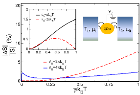
Figure 1: Main panel: The relative discrepancy in thermopower, $\Delta S/S$, defined as $(S_{exact}-S_{protocol})/S_{exact}$ (computed using equations 5 and  9) is plotted as a function of $\gamma/k_{B}T$ for non-zero $\epsilon_{0}=4\pi k_{B}T$ (blue solid line) and $2\pi k_{B}T$ (red dashed line) at $T=3$ K and $\Theta=0.1$ K. Inset: The same quantity is calculated in the nonlinear regime at $T=3$ K and $\Theta=3$ K NL_parameters . The relative discrepancy reduces to 1-2% in the nonlinear regime thus offering an improved standard. The schematic represents the relevance of this protocol for quantum dot devices.

We have bench marked the expression used for this protocol in Fig. (1), where we show the difference between the protocol expression equation (9) and the exact result equation (5) as a function of the scaled width $\gamma/k_{B}T$ for various resonant level positions. It is seen that the discrepancy, $\Delta S/S$, between the exact (equation (5)) and the protocol expression (equation (9)) is less than 4% for an $\epsilon_{0}$ as large as $2\pi k_{B}T$. In fact an analysis of thermopower tells us that the discrepancy, $\Delta S$ reduces dramatically in the nonlinear regime thus offering an even better protocol. This is seen in the inset of fig. (1) where $\Delta S$ is seen to decrease in the presence of a finite thermal bias (as compared to the main panel). We have seen that the discrepancy between the protocol and exact thermopower offset near $\epsilon_{0}\rightarrow 0$ can be as large as $20\%$, and is hence less reliable (see Figure (4) in SM NR_SI ).

Broad Resonance:

The broad resonance transmission defined by $\gamma\gg k_{B}T_{L},$ $k_{B}T_{R}$ is most appropriate for molecular junctions where the HOMO and LUMO levels are broadened due to the coupling with the leads, and the width of these levels could easily be of the order of eV, which is far greater than the thermal energy scales. Further, since the HOMO-LUMO level separation is much greater compared to the width or the thermal energy scale, a single resonance $L(\epsilon)$ can again be assumed. It is easy to see that in equation (3), if $\bar{\gamma}_{L/R}\gg 1$, then $|z_{L/R}|\gg 1$ irrespective of the values of the $\epsilon_{0}$ or the bias, since the latter are present in the imaginary part, while $\gamma$ is in the real part of $z_{L/R}$. This allows us to use the asymptotic form of digamma function Stegun for large $z$, which is $\Psi(z)\sim\ln z-1/z;z\rightarrow\infty,|{\rm arg}(z)|<\pi$. Hence, we get for $I$ in units of $2e/h$,

$$I= \sum_{r}\bigg{\{}\gamma_{r}\left[\mathrm{tan}^{-1}\left(\frac{-\lambda_{r-}}{\gamma_{r}}\right)+\mathrm{tan}^{-1}\left(\frac{\lambda_{r+}}{\gamma_{r}}\right)\right]$$

$$+ \frac{\gamma_{r}^{2}\pi^{2}k_{B}^{2}}{3}\bigg{[}\frac{T_{L}^{2}\lambda_{r-}}{(\gamma_{r}^{2}+\lambda_{r-}^{2})^{2}}-\frac{T_{R}^{2}\lambda_{r+}}{(\gamma^{2}+\lambda_{r+}^{2})^{2}}\bigg{]}\bigg{\}},$$ (10)

where, $\lambda_{r,\pm}=\epsilon_{r}\pm eV/2$. As the above arguments show, this equation is valid for arbitrary values of the resonance position $\bar{\epsilon}$ or the voltage bias $\bar{V}$ as long as $\bar{\gamma}\gg 1$ is satisfied implying that it is sufficient for the thermal energy scales to be much smaller compared to the resonance width. Although the above arguments seems to be based upon a broad resonance condition, a subtle point to note is that this form may be applied for arbitrary widths ($\gamma/k_{B}T$) if the magnitude of the level position (measured from the chemical potential) is large compared to $\mathrm{max}(eV/2,k_{B}T)$, thus making it useful for molecular junctions. The result obtained here represents a generalization of an expression obtained by Stafford Stafford1996 ; Ioan2012 , (for RTFs in the wide band approximation) at $T=0$ to finite temperatures and a finite thermal bias. We can now clearly see through eq (10), the emergence of a temperature controlled current rectifier. This rectification current, defined as $\Delta I=(I(V,T_{L},T_{R})+I(-V,T_{L},T_{R}))/2$ in units of $\frac{2e}{h}$ is given by,

$$\Delta I=\sum_{r}\frac{\gamma_{r}^{2}\pi^{2}k_{B}^{2}}{3}T\Theta\left[\frac{\lambda_{+}}{(\gamma_{r}^{2}+\lambda_{+}^{2})^{2}}+\frac{\lambda_{-}}{(\gamma_{r}^{2}+\lambda_{-}^{2})^{2}}\right]$$ (11)

This rectification current is experimentally measurable ($\sim$ nA) (Figure (3) in SM BR_SI ) even at a temperature and thermal bias of $50$ K each. This motivates us to design a protocol for predicting the resonant transmission function parameters through $\Delta I$ at zero voltage bias (which is in fact the thermocurrent, $\Delta I_{th}$) in conjunction with the zero bias conductance. This protocol involving the thermocurrent ($\Delta I_{th}$) shall be discussed below.

The existing protocol for finding the resonant level in molecular junctions is implemented through transition voltage spectroscopy (TVS) TVS1Yu ; TVS2Liu ; Beebe2006 ; Beebe2008 ; Tan2010 . The basis for this protocol is the existence of a minimum, in the $\ln~{}(I/V^{2})$ versus $1/V$ curve. This minimum is useful because, it occurs at a voltage that is much smaller and accessible than the resonance condition voltage ($V=2\epsilon_{0}$). The interpretation of this voltage minimum as $V_{m}^{conv}=2\epsilon_{0}/\sqrt{3}$ relies on a result  Ioan2012 obtained in the limit when $\gamma/\epsilon_{0}\ll 1$, and hence the information on the width of the resonance is completely lost. We have obtained a result for the TVS minimum that is valid for a regime where $\gamma/\epsilon_{0}$ may be significant (e. g. amine linked junctions) Hybertsen2008 ; Hybertsen2007 , which is,

$$\frac{eV_{m}}{\epsilon_{0}}=\frac{eV_{m}^{conv}}{\epsilon_{0}}\left[1+5\left(\frac{\gamma}{\epsilon_{0}}\right)^{2}\right]^{1/2}\,.$$ (12)

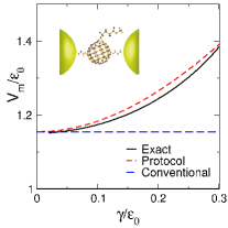
Figure 2: Comparison of TVS minimum, $V_{m}$, obtained using the protocol equation (12) (red dashed line), exact solution BR_SI (black solid line) and the conventional Ioan2012 $V_{m}^{conv}=2\epsilon_{0}/\sqrt{3}$ (blue dashed line). The schematic in the inset represents a molecular junction.

A comparison between the $V_{m}$ obtained and the $V_{m}^{conv}$ with the exact result BR_SI as obtained by numerically finding the minimum is shown in fig. (2). It is seen that the deviation from the conventional TVS minimum occurs even at very small widths ($\gamma/\epsilon_{0}\sim 0.05$), while the agreement with the exact result is excellent. Thus the experimentally measured $V_{m}$ would contain information about both $\epsilon_{0}$ and $\gamma$ and hence by itself, cannot be used to find the level position and the width. A second equation is needed that relates an experimentally measurable quantity to $\epsilon_{0}$ and $\gamma$. We state that such a quantity is the ratio $R_{TVS}$ of $\Delta I_{th}$ to the zero bias conductance $G$. The latter (obtained either by using equation (4) or using equation (10), for a single resonance with $T_{L}=T_{R}=T$ is given by

$$G=\frac{2e^{2}\gamma^{2}}{h}\left[\frac{1}{2(\gamma^{2}+\lambda_{+}^{2})}+\frac{1}{2(\gamma^{2}+\lambda_{-}^{2})}\right].$$ (13)

and hence the ratio is given by:

$$R_{TVS}=\frac{\Delta I_{th}}{G}=\frac{k_{B}^{2}\pi^{2}}{3e}\frac{4T\Theta\epsilon_{0}}{(\gamma^{2}+\epsilon_{0}^{2})}\,.$$ (14)

Equations (12) and (14) can be easily combined to get both $\gamma$ and $\epsilon_{0}$. So if we define $X=\sqrt{3}eV_{m}/2$ and $Y=3eR_{TVS}/(4\pi^{2}T\Theta)$, which are experimentally measurable, then $\gamma$ and $\epsilon_{0}$ may be obtained through simple expressions involving $X$ and $Y$ BR_SI .

Finite width:

In the final part, we provide expressions for the $I-V$ characteristic in the finite width regime ($\gamma\sim k_{B}T$), which has hitherto been analytically inaccessible. We can utilize the recurrence relations and the multiplication formula for the digamma function Stegun to get the following result. If $T_{L}=T_{R}=T$ and $\gamma_{r}=n\pi k_{B}T;\;n=1,2,...$, then the current $I$ in units of $2e/h$ is given by, for $n=2m+1$

$$I= \sum_{r}\bigg{[}\frac{\pi}{\alpha_{L}}-\frac{\pi}{\alpha_{R}}+\frac{\pi}{2}\left(\coth(\pi\alpha_{Lr})-\coth(\pi\alpha_{Rr})\right)+$$

$$\sum_{rk=0}^{m}\left\{\frac{\alpha_{Lr}}{k^{2}+|\nu_{L}|^{2}}-\frac{\alpha_{Rr}}{k^{2}+|\nu_{R}|^{2}}\right\}\bigg{]},$$

where, $\nu_{L/R}=-\frac{i\alpha_{L/R}}{2\pi}$. The case for $n=2m$ can also be similarly derived FW .

Finding the $L(\epsilon)$ for systems where electron-electron and electron-phonon interactions play a dominant role, is of course a major bottleneck and is currently a major topic of research Ness2010 ; Sanvito2012 ; benzene ; Kotliar2010 ; Markussennanolett ; Stafford2009 ; DiVentra . Nevertheless, it is clear from our work that expressing the local properties of the interacting region ($L(\epsilon)$) in terms of RTFs allows the utilization of exact results. Subsequently, we have proposed substantially improved protocols that can be implemented experimentally for finding transmission function parameters in quantum dots and molecular junctions. Our results being based on exact solutions also provide analytical insight into the difficult nonlinear regime, and provide a unified platform for the analysis of simulations and experiments in quantum transport through nanostructures.

- (1) R. Landauer, IBM. J. Res. Dev 1, 233 (1957)
- (2) R. Landauer, Philos. Mag. 21, 863 (1970)
- (3) M. Bttiker, Phys. Rev. Lett 57, 1761 (1986)
- (4) Y. Meir and N. S. Wingreen, Phys. Rev. Lett. 68, 2512 (1992)
- (5) H. Ness, L. K. Dash, and R. W. Godby, Phys. Rev. B 82, 085426 (2010)
- (6) M. Galperin, A. Nitzan, S. Sek, and M. Majda, Journal of Electroanalytical Chemistry 550, 337 (2003)
- (7) B. R. Bułka and T. Kostyrko, Phys. Rev. B 70, 205333 (2004)
- (8) A. T. Johnson, L. P. Kouwenhoven, W. de Jong, N. C. van der Vaart, C. J. P. M. Harmans, and C. T. Foxon, Phys. Rev. Lett. 69, 1592 (1992)
- (9) E. B. Foxman, P. L. McEuen, U. Meirav, N. S.Wingreen, Y. Meir, P. A. Belk, N. R. Belk, and M. A. Kastner, Phys. Rev. B 47, 10020 (1993)
- (10) P. Reddy, S.-Y. Jang, R. A. Segalman, and A. Majumdar, Science 315, 1568 (2007)
- (11) H. W. C. Postma, T. Teepen, Z. Yao, M. Grifoni, and C. Dekker, Science 293, 76 (2001)
- (12) S. F. Svensson, A. I. Persson, E. A. Hoffmann, N. Nakpathomkun, H. A. Nilsson, H. Q. Xu, L. Samuelson, and H. Linke, New. J. Phys 14, 033041 (2012)
- (13) J. Chen, T. Markussen, and K. S. Thygesen, Phys. Rev. B 82, 121412(R) (2010)
- (14) C. A. Stafford, Phys. Rev. Lett. 77, 2770 (1996)
- (15) T. Christen and M. Bttiker, Europhys. Lett. 35, 523 (1996)
- (16) N. L. Dickens and D. E. Logan, J. Phys:. Condens. Matter 13, 4505 (2001)
- (17) M. Abramowitz and I. A. Stegun, Handbook of Mathematical Functions with Formulas, Graphs, and Mathematical Tables, ninth dover printing, tenth gpo printing ed. (Dover, New York, 1964)
- (18) P. Murphy, S. Mukerjee, , and J. Moore, Phys. Rev. B 78, 161406(R) (2008)
- (19) T. Rejec, R. Zitko, J. Mravlje, and A. Ramsak, Phys. Rev. B 85, 085117 (2012)
- (20) See Supplemental Material at [URL will be inserted by publisher] for the identites provided in Section IV
- (21) N. B. Kopnin, Y. M. Galperin, and V. M. Vinokur, Phys. Rev. B 79, 035319 (2009)
- (22) C. W. J. Beenakker, Phys. Rev. B 44, 1646 (1991)
- (23) P. Mani, N. Nakpathomkun, E. A. Hoffmann, and H. Linke, Nano Lett. 11, 4679 (2011)
- (24) See Supplemental Material at [URL will be inserted by publisher] for detailed derivations and expressions and additional figures relevant for the narrow resonance regime in Section II
- (25) MATLAB, version 7.10.0 (R2010a) (The MathWorks Inc., Natick, Massachusetts, 2010)
- (26) These parameters are justified within our theory and are experimentally feasible within the specified approximations, for e.g see Linke2012 .
- (27) I. Bldea, Phys. Rev. B 85, 035442 (2012)
- (28) See Supplemental Material at [URL will be inserted by publisher] for detailed derivations and expressions and additional figures relevant for the broad resonance regime in Section III
- (29) L. H. Yu, N. Gergel-Hackett, C. D. Zangmeister, C. A. Hacker, C. A. Richter, and J. G. Kushmerick, J. Phys. Condens. Matter 20, 374114 (2008)
- (30) K. Liu, X. Wang, and F. Wang, ACS Nano 2, 2315 (2008)
- (31) J. M. Beebe, B. Kim, J. W. Gadzuk, C. D. Frisbie, and J. G. Kushmerick, Phys. Rev. Lett. 97, 026801 (2006)
- (32) J. M. Beebe, B. Kim, C. D. Frisbie, and J. G. Kushmerick, ACS Nano 2, 827 (2008)
- (33) A. Tan, S. Sadat, and P. Reddy, Appl. Phys. Lett. 96, 013110 (2010)
- (34) M. S. Hybertsen, L. Venkataraman, J. E. Klare, A. CWhalley, M. L. Steigerwald, and C. Nuckolls, J. Phys: Condens. Matter 20, 374115 (2008)
- (35) S. Y. Quek, L. Venkataraman, H. J. Choi, S. G. Louie, M. S. Hybertsen, and J. B. Neaton, Nano Lett. 7, 3477 (2007)
- (36) See Supplemental Material at [URL will be inserted by publisher] for the derivation.
- (37) J.-X. Yu, X.-R. Chen, S. Sanvito, and Y. Cheng, Appl. Phys. Lett. 100, 013113 (2012)
- (38) Y. Li, P. Wei, M. Bai, Z. Shen, S. Sanvito, and S. Hou, Chem. Phys. 397, 82 (2012)
- (39) D. Jacob, K. Haule, and G. Kotliar, Phys. Rev. B 82, 195115 (2010)
- (40) T. Markussen, R. Stadler, and K. S. Thygesen, Nano Lett. 10, 4260 (2010)
- (41) J. P. Bergfield and C. A. Stafford, Phys. Rev. B 79, 245125 (2009)
- (42) M. Brandbyge, J.-L. Mozos, P. Ordejon, J. Taylor, and K. Stokbro, Phys. Rev. B 65, 165401 (2002)