Critical Properties of the Kitaev-Heisenberg Model

Abstract

We study the critical properties of the Kitaev-Heisenberg (KH) model on the honeycomb lattice at finite temperatures that might describe the physics of the quasi two-dimensional (2D) compounds, Na₂IrO₃ and Li₂IrO₃. The model undergoes two phase transitions as a function of temperature. At low temperature, thermal fluctuations induce magnetic long-range order by the order-by-disorder mechanism. This magnetically ordered state with a spontaneously broken $Z_{6}$ symmetry persists up to a certain critical temperature. We find that there is an intermediate phase between the low-temperature, ordered phase and the high-temperature, disordered phase. Finite-sized scaling analysis suggests that the intermediate phase is a critical Kosterlitz-Thouless (KT) phase with continuously variable exponents. We argue that the intermediate phase has been observed above the low-temperature, magnetically ordered phase in Na₂IrO₃, and also likely exists in Li₂IrO₃.

Introduction. The Ir-based transition metal oxides, in which the orbital degeneracy is accompanied by a strong relativistic spin-orbit coupling (SOC), have recently attracted a lot of theoretical and experimental attention nakatsuji06 ; okamoto07 ; kim09 ; gegenwart10 ; gegenwart12 ; liu11 ; choi12 ; takagi11 . This is because the strong SOC creates a different, and frequently novel, set of magnetic and orbital states due to the unusual anisotropic exchange interactions between localized moments which are in turn determined by the combination of spin and lattice symmetries. The spin-orbital models that describe the low-energy physics of iridium systems often include anisotropic terms that do not reduce to the conventional easy-plane and easy-axis anisotropies because they involve the products of different components of multiple spin operators. These terms are responsible for exotic Mott-insulating states kim09 , topological insulators Shitade09 ; Pesin10 , spin-orbital liquid states nakatsuji06 ; okamoto07 , and non-trivial long-range magnetic orders kim09 ; gegenwart10 ; liu11 .

A prominent example of such an anisotropic spin-orbital model is the KH model on the honeycomb lattice jackeli09 ; jackeli10 which likely describes the low-energy physics of the quasi 2D compounds, Na₂IrO₃ and Li₂IrO₃. In these compounds, Ir⁴⁺ ions are in a low spin $5d^{5}$ configuration and form weakly coupled hexagonal layers gegenwart10 ; liu11 ; takagi11 . Due to strong SOC, the atomic ground state is a doublet where the spin and orbital angular momenta of Ir⁴⁺ ions are coupled into $J_{\rm eff}=1/2$. It was suggested jackeli09 ; jackeli10 that the interactions between these effective moments can be described by a spin Hamiltonian containing two competing nearest neighbor (NN) interactions: an isotropic antiferromagnetic (AF) Heisenberg exchange interaction and a highly anisotropic ferromagnetic (FM) Kitaev exchange interaction kitaev06 . This competition can be described with the parameter, $0\leq\alpha\leq 1$, which sets the relative strength of these two interactions. At $\alpha=0$, the coupling corresponds to the AF Heisenberg interaction, and at $\alpha=1$, it corresponds to the Kitaev interaction.

This model immediately attracted a lot of attention; several theoretical studies were published in the last few years jackeli10 ; jiang11 ; reuther11 ; trousselet11 on both the ground state and its properties at finite temperature. The ground state phase diagram of the KH model exhibits three distinct phases: the AF Néel phase for small $\alpha\in(0.,0.4)$, the stripy AF phase for intermediate $\alpha\in(0.4,0.86)$, and the disordered spin-liquid phase at large $\alpha\in(0.86,1.)$. While the phase transition between the Néel and the stripy phase appears to be discontinuous, numerical studies including density matrix renormalization group jiang11 and exact diagonalization results jackeli10 suggest that the transition between the spin liquid and the stripy state is continuous or weakly first-order. Additionally, quantum fluctuations select all of the magnetically ordered phases to have the order parameter point along one of the cubic axes.

In this Letter, we discuss finite temperature properties of the KH model on the honeycomb lattice. A first step in this direction was made in Ref. reuther11 , where the critical ordering scale for the magnetically ordered states was analyzed using a pseudofermion functional renormalization group approach. Here we present numerical results obtained using Monte Carlo (MC) simulations. We study the classical KH model because the corresponding quantum model has a sign problem precluding quantum MC analysis and also because the existence of long-range order at low temperatures in Na₂IrO₃ and in Li₂IrO₃ indicates that quantum fluctuations are not dominating in these materials gegenwart10 ; gegenwart12 ; liu11 ; choi12 ; takagi11 .

We show that the thermal fluctuations of classical spins give rise to two distinct temperature dependent effects. At low temperature they predominantly act as the source of the order-by-disorder phenomenon and select collinear magnetic order where the spins are oriented along one of the cubic directions. There are six possible ordered states, one of which is spontaneously chosen by the system. At high temperatures, when $T$ is larger than any energy scale in the system, the fluctuations destroy any order putting the KH model into a three dimensional paramagnetic state. The main goal of our study is to see how these two phases are connected.

We argue that the classical KH model effectively behaves like a six-state clock model jose77 ; isakov03 ; chern12 ; ortiz12 and that it undergoes two continuous phase transitions as a function of temperature separating three phases: a low-T ordered phase, an intermediate critical phase, and a high-T disordered phase. The critical phase has an emergent, continuous $U(1)$ symmetry which is fully analogous to the low-T phase of the XY model, a well-known KT phase of critical points with floating exponents and algebraic correlations. Here we present numerical data only for $\alpha=0.25$ and $\alpha=0.75$ since these values likely characterize the ratio between the AF Heisenberg interaction and the Kitaev interaction in Na₂IrO₃ and Li₂IrO₃. However, we note that recent inelastic neutron scattering measurements on Na₂IrO₃ have shown that the KH model alone is insufficient to describe the magnetic properties of this compound choi12 . It has been demonstrated that it is essential to include substantial further-neighbor exchanges to describe both the zigzag ground state and the excitation spectrum in Na₂IrO₃. The full finite-temperature phase diagram for the KH model with second and third neighbor exchange interactions will be published elsewhere unpublished .

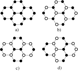
Figure 1: Four possible magnetic configurations: (a) the FM ordering; (b) the two-sublattice, AF Néel order; (c) the stripy order; (d) the zigzag order. Open and filled circles correspond to up and down directions of spins.

The Model. The classical version of the KH model which describes the interactions among the $J=1/2$ degrees of freedom of Ir⁴⁺ ions reads as

$$\mathcal{H}=-J_{K}\sum_{\langle ij\rangle_{\gamma}}S_{i}^{\gamma}S_{j}^{\gamma}+J_{H}\sum_{\langle ij\rangle}{\bf S}_{i}{\bf S}_{j}~{}.$$ (1)

where the spin quantization axes are taken along the cubic axes of the IrO₆ octahedra. $\gamma=x,y,z$ denotes the three bonds of the honeycomb lattice. The exchange constants, $J_{K}=2\alpha$ and $J_{H}=1-\alpha$, correspond to the Kitaev and Heisenberg interactions which can be derived from a multiorbital Hubbard Hamiltonian jackeli10 .

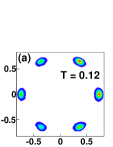
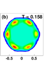
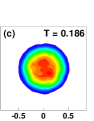
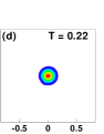
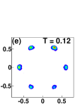
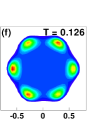
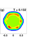
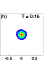
Figure 2: Histograms of the order parameter $m_{N(S)}$, obtained for the system with 2*84*84 spins in the ordered phase, (a) and (e), in the intermediate phase, (b)-(c) and (f)-(g), and in the disordered phase, (d) and (h). Histograms (a)-(d) are computed for $\alpha=0.25$, and (e)-(h) are for $\alpha=0.75$. The histograms are presented on the complex plane (Re $|m_{N(S)}|$, Im $|m_{N(S)}|$).

Order by Disorder. The symmetry of the KH model combines the cubic symmetry of both the spin and the lattice space. It consists of simultaneous permutations between the $x,y,z$ spin components and a $C_{3}$-rotation of the lattice which defines a discrete symmetry. The classical ground state has a higher symmetry than that of the Hamiltonian – the ground state energy does not change under a simultaneous rotation of all spins. Since this applies only to the ground state,the KH model has only an accidental continuous rotation symmetry. Its actual symmetry is discrete; at zero temperature, the ”pseudo” SU(2) symmetry is broken by quantum fluctuations that restore the underlying cubic symmetry of the model jackeli10 . The magnetically ordered phase is gapped with a spin gap that corresponds to the finite energy cost of deviating the order parameter from one of the cubic axes. We show in the following that thermal fluctuations of classical spins at finite T also select a collinear spin configuration whose order parameter points along one of the cubic axes.

Parameters of the Simulations. We have carried out classical MC simulations of the model (1) using the standard Metropolis algorithm. In our MC simulations, we treat the spins as three-dimensional (3D) vectors, ${\bf S}_{i}=(S_{i}^{x},S_{i}^{y},S_{i}^{z})$, of unit magnitude with $(S_{i}^{x})^{2}+(S_{i}^{y})^{2}+(S_{i}^{z})^{2}=1$ at every site. At each temperature, more than $10^{7}$ MC sweeps were performed. Of these, $5*10^{5}$ were used to equilibrate the system, and afterwards only 1 out of every 5 sweeps was used to calculate the averages of physical quantities. We present all energies in the units of $J_{H}$ and assume $k_{B}=1$. The calculations were carried out on several finite systems with size $2*L*L$ that are spanned by the primitive vectors of a triangular lattice ${\bf a}_{1}=(1/2,\sqrt{3}/2)$ and ${\bf a}_{2}=(1,0)$ with a 2-point basis using periodic boundary conditions.

Results. To study the possible phases of the model (1), we introduce four magnetic configurations (Fig. 1): a FM order, a simple two-sublattice AF Néel order, a stripy order, and a zigzag spin order. The classical energies of these states can be easily computed: $E_{cl}^{\mathcal{M}}=3-5\alpha$, $E_{cl}^{\mathcal{Z}}=-3\alpha+1$, $E_{cl}^{\mathcal{S}}=-\alpha-1$, and $E_{cl}^{\mathcal{N}}=5\alpha-3$ for the FM, the zigzag, the stripy and the Néel phases, respectively. For $0\leq\alpha<1$, the classical ground state is either the Néel AF with the vector order parameter $\mathcal{N}=\frac{1}{N}\sum_{i}({\bf S}_{iA}-{\bf S}_{iB})$ or the stripy phase described by $\mathcal{S}=\frac{1}{N}\sum_{i=n}({\bf S}_{iA}-{\bf S}_{iB}+{\bf S}_{iC}-{\bf S}_{iD})$. Here, $A,B$ and $A,B,C,D$ denote either two or four sublattices that respectively characterize the Néel AF and stripy order. The classical phase transition between them occurs at $\alpha=1/3$. At $\alpha=1$, the FM, stripy, and zigzag phases all have the same classical energy. However, the classical degeneracy of this point, which corresponds to the pure Kitaev model, is much higher. This limit has been thoroughly studied by Baskaran et al. baskaran08 .

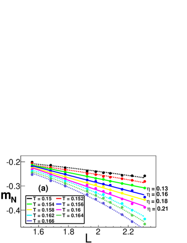
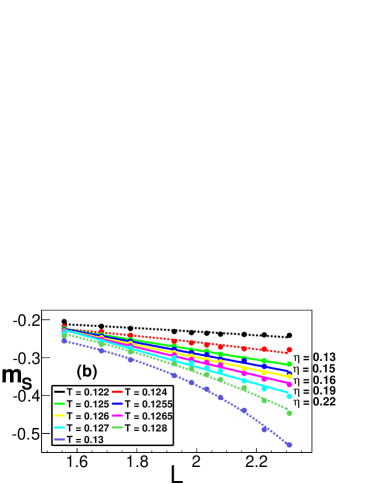
Figure 3: The log-log plots of the order parameter $m_{N(S)}$ as a function of system size $L$ at various temperatures. The solid curves indicate the linear behavior that corresponds to a power-law dependence, $m_{N(S)}\sim L^{-\eta/2}$, cooresponding to the intermediate critical phase. The dashed curves show deviation away from the linear behavior outside the critical phase.

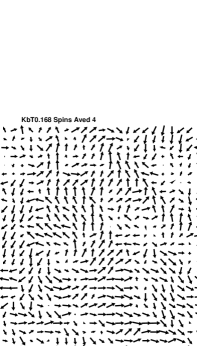
Figure 4: A snapshot of the coarse-grained order parameter $\langle m_{N}\rangle$ at $T=0.168$. The vortex-like topological excitations are evident.

To make an analogy to the six-state clock model, we map the order parameter describing the magnetically ordered phase of the KH model onto a 2D complex order parameter, $m_{N(S)}=\sum_{i=1}^{6}|m_{i,N(S)}|e^{\imath\theta_{i}}$, such that the six possible ordered states are characterized by $\theta_{i}=\pi n_{i}/3$, $n_{i}=0,..5$ chern12 . The mapping is exact only well within the ordered state since there is no guarantee that the thermal fluctuations of the order parameter will actually have a 2D character given that the spin degrees of freedom are three-dimensional. Depending on the strength of the spin stiffness in different directions, the long-range low-T magnetic order can be destroyed in one of several ways. If the stiffness of thermal fluctuations along the circle is softer than the stiffness of fluctuations in the direction transverse to the circle, the long-range order may be destroyed by a discontinuous first-order transition, by two continuous phase transitions with an intermediate partially ordered phase, or by two KT phase transitions with an intermediate critical phase jose77 ; isakov03 ; chern12 ; ortiz12 . In the last scenario, the critical phase is destroyed by topological excitations in the form of discrete vortices whose existence is directly related to the emergence of a continuous symmetry; the high-T transition will first bring the system into a disordered phase where fluctuations are primarily 2D, and the crossover to the 3D paramagnet occurs at even higher temperatures.

In Fig. 2 we present the results of the histogram method for the complex order parameter. At low temperatures, Figs. 2 (a) and (e), a sixfold degeneracy present in the ordered phase is seen. For both $\alpha=0.25$ and $\alpha=0.75$, the six states which have the highest weight in the histogram are where the order parameter $m_{N(S)}$ points along one of the cubic axes. In Figs. 2 (b) and (f), when the temperature increases beyond a certain critical temperature, a continuous $U(1)$ symmetry emerges signaling both the disappearance of the sixfold anisotropy and the appearance of the critical phase. The formation of vortices can be seen in Fig. 4 where we present a snapshot of the coarse-grained order parameter $\langle m_{N}\rangle$ at $T=0.168$. Upon a further increase in temperature, the amplitude of the order parameter decreases (Figs. 2 (c) and (g)) until it shrinks to zero indicating the transition to the paramagnetic phase (Figs. 2 (d) and (h)).

To better understand the properties of the intermediate phase and to confirm its critical nature, we performed the finite-size scaling analysis appropriate for KT transitions challa86 . The full finite-size scaling analysis is rather involved and will be reported elsewhere unpublished . Here we present only the scaling behavior of the order parameter. At the KT transition, the order parameter exhibits the power law dependence on system size, $m\sim L^{-\eta/2}$. As each point of the intermediate critical phase can be understood as a critical point, the power law behavior of the order parameter should hold throughout the entire phase. We found that the boundaries of the critical phase are characterized by critical exponents close to $1/9$ and $1/4$ for the lower and upper boundaries at $T_{c_{1}}$ and $T_{c_{2}}$, which is in agreement with critical exponents for the six-state clock model obtained by the renormalization group analysis jose77 . Fig. 3 shows the log-log plots of the order parameter $m_{N(S)}$ as a function of system size for different temperatures. For $\alpha=0.25$, the data points in Fig. 3 a) show a linear behavior in the temperature interval between $T_{c_{1}}\simeq 0.152$ and $T_{c_{2}}\simeq 0.162$, in which there are several critical lines characterized by $\eta$ between $1/9$ and $1/4$. For $\alpha=0.75$, we have detected the critical phase in the temperature interval between $T_{c_{1}}\simeq 0.125$ and $T_{c_{2}}\simeq 0.127$.

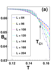
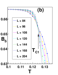
Figure 5: The Binder cumulant as a function of temperature for (a) $\alpha=0.25$ and (b) $\alpha=0.75$. From the crossing points of different Binder’s curves, we estimate $T_{c_{1}}=0.152$ and $T_{c_{1}}=0.124$ for $\alpha=0.25$ and $\alpha=0.75$, respectively.

The lower transition temperature $T_{c_{1}}$ can be independently determined using fourth-order Binder cumulant (Figs. 5 (a) and (b)). The Binder cumulant has a scaling dimension of zero; thus the crossing point of the cumulants for different lattice sizes provides a reliable estimate for the value of the critical temperature $T_{c_{1}}$ at which the long range order is destroyed. The crossing points for $\alpha=0.25$ and $\alpha=0.75$ are $T_{c_{1}}=0.152$ and $T_{c_{1}}=0.124$, respectively. They are in good agreement with estimates obtained from the log-log plots in Fig. 3.

In Figs. 6 (a) and (b) we present the temperature dependence of the specific heat, $C=(\langle E^{2}\rangle-\langle E\rangle^{2})/NT^{2}$. While the low-T transition, seen as small peak at temperatures $T_{c_{1}}=0.152$ and $0.1247$ for $\alpha=0.25$ and $0.75$, respectively, is in a good agreement with our previous estimates, the features corresponding to the high-T transition $T_{c_{2}}$ are barely distinguished by eye. This is not surprising as the high-T transition is a usual KT transition at which the specific heat does not diverge at the critical point last . It is also likely that the high-T KT transition might be shadowed by the crossover to the 3D paramagnet, which is seen in Fig. 6 as a very broad hump at higher-T.

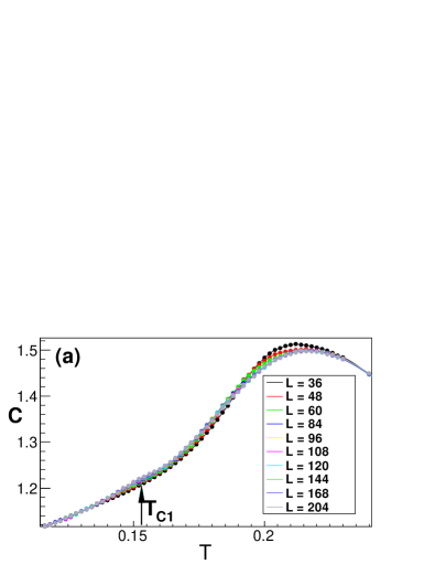
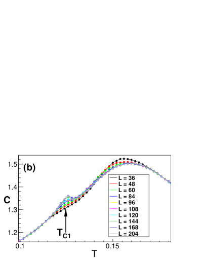
Figure 6: Specific heat $C$ as a function of temperature for (a) $\alpha=0.25$ and (b) $\alpha=0.75$.

Our findings for the specific heat show a lot of similarities between the experimental data obtained on the Na₂IrO₃ and Li₂IrO₃ compounds by Refs. gegenwart10 ; gegenwart12 and takagi11 . In Na₂IrO₃, both the lambda-like anomaly at the Néel ordering temperature, $T_{N}=15$ K, and a broad tail which extends into higher temperatures are seen in the specific heat measurements gegenwart10 . The latter suggests the presence of short-range order above the bulk 3D ordering that can be understood by our proposed scenario of the critical phase.

Let us estimate the temperatures of the KT transitions and the width of the critical phase in Na₂IrO₃ based on our results obtained for the KH model with $\alpha=0.25$. On the mean field level, the exchange on the NN bonds may be estimated from the classical energy, $J_{1}\simeq(3-5\alpha)/3$, in the Néel phase. From the recent neutron scattering experiment choi12 , the NN exchange in Na₂IrO₃ was estimated to be $J_{1}=4.17$ meV. In the bulk of our paper, all energies were measured in the units of $J_{H}$, and thus we estimate $J_{1}$ to be equal to 12.7 meV. This gives the prediction for the critical temperature to be $T_{c_{1}}=16.8$ K, which is very close to the experimental value $T_{N}=15$ K gegenwart10 ; gegenwart12 . Our estimate for the upper boundary of the critical phase is $T_{c_{2}}=17.7$ K which makes the predicted critical phase very narrow. We note here that the critical phase survives in the extended KH model with included further-neighbor exchange couplings choi12 ; gegenwart12 ; mazin12 which are essential for comparison with experiment. However, in order to determine the upper boundary of the critical phase additional extensive numerical simulations must be performed.

Acknowledgements. The authors are particularly thankful to C. Batista, G.-W. Chern, G. Jackeli, and Y. Kato for stimulating discussions and many helpful suggestions. We are grateful to H. Takagi and T. Takayama for sharing with us unpublished data on Na₂IrO₃ and Li₂IrO₃. N.P. acknowledges the support from NSF grant DMR-1005932. N.P. also thanks the hospitality of the visitors program at MPIPKS, where the part of the work has been done.

References

- (1) S. Nakatsuji et al., Phys. Rev. Lett. 96, 087204 (2006).
- (2) Y. Okamoto et al., Phys. Rev. Lett. 99, 137207 (2007).
- (3) B. J. Kim et al., Science 323, 1329 (2009).
- (4) Y. Singh and P. Gegenwart, Phys. Rev. B 82, 064412 (2010).
- (5) Yogesh Singh et al., Phys. Rev. Lett. 108, 127203 (2012)
- (6) X. Liu et al., Phys. Rev. B 83, 220403(R) (2011).
- (7) S. K. Choi et al., Phys. Rev. Lett. 108, 127204 (2012).
- (8) H. Takagi, unpublished.
- (9) G.-W. Chern and N. B. Perkins, Phys. Rev. B 80, 180409(R) (2009).
- (10) A. Shitade et al., Phys. Rev. Lett. 102, 256403 (2009).
- (11) D.Pesin, L.Balents, Nature Physics 6, 376 (2010).
- (12) G. Jackeli and G. Khaliullin, Phys. Rev. Lett. 102, 017205 (2009).
- (13) J. Chaloupka, G. Jackeli, and G. Khaliullin, Phys. Rev. Lett. 105, 027204 (2010).
- (14) A. Kitaev, Ann. Phys. 321, 2 (2006).
- (15) H.-C. Jiang, Z.-C. Gu, X.-L. Qi, and Simon Trebst Phys. Rev. B 83, 245104 (2011).
- (16) J. Reuther, R. Thomale, and S. Trebst, Phys. Rev. B 84, 100406 (2011).
- (17) F. Trousselet, G. Khaliullin, P. Horsch, Phys. Rev. B 84, 054409 (2011).
- (18) J.V. José, L.P. Kadanoff, S. Kirkpatrick S and D. R. Nelson, Phys. Rev. B 16, 1217 (1977).
- (19) S. V. Isakov and R. Moessner, Phys. Rev. B68, 104409 (2003).
- (20) G.-W. Chern, O. Tchernyshyov, arXiv:1109.0275.
- (21) G. Ortiz, E. Cobanera, Z. Nussinov, Nuclear Physics B 854, 780 (2012).
- (22) G. Baskaran, D. Sen, and R. Shankar, Phys. Rev. B 78, 115116 (2008).
- (23) C.Price and N.B.Perkins, unpublished.
- (24) M.S.S. Challa and D.P. Landau, Phys. Rev. B 33, 437 (1986).
- (25) I. I. Mazin et al., arXiv:1205.0434
- (26) Fabien Aletet al., Phys. Rev. E 74, 041124 (2006).