Proton, Electron, and Ion Heating in the Fast Solar Wind from Nonlinear Coupling Between Alfvénic and Fast-Mode Turbulence

Abstract

In the parts of the solar corona and solar wind that experience the fewest Coulomb collisions, the component proton, electron, and heavy ion populations are not in thermal equilibrium with one another. Observed differences in temperatures, outflow speeds, and velocity distribution anisotropies are useful constraints on proposed explanations for how the plasma is heated and accelerated. This paper presents new predictions of the rates of collisionless heating for each particle species, in which the energy input is assumed to come from magnetohydrodynamic (MHD) turbulence. We first created an empirical description of the radial evolution of Alfvén, fast-mode, and slow-mode MHD waves. This model provides the total wave power in each mode as a function of distance along an expanding flux tube in the high-speed solar wind. Next we solved a set of cascade advection-diffusion equations that give the time-steady wavenumber spectra at each distance. An approximate term for nonlinear coupling between the Alfvén and fast-mode fluctuations is included. For reasonable choices of the parameters, our model contains enough energy transfer from the fast mode to the Alfvén mode to excite the high-frequency ion cyclotron resonance. This resonance is efficient at heating protons and other ions in the direction perpendicular to the background magnetic field, and our model predicts heating rates for these species that agree well with both spectroscopic and in situ measurements. Nonetheless, the high-frequency waves comprise only a small part of the total Alfvénic fluctuation spectrum, which remains highly two-dimensional as is observed in interplanetary space.

1. Introduction

The energy that heats the solar corona and accelerates the solar wind originates in convective motions beneath the Sun’s surface. However, even after many years of investigation, the physical processes that transport a fraction of this energy to the corona and convert it into thermal, magnetic, and kinetic energy are still not understood. In order to construct and test theoretical models, a wide range of measurements of relevant plasma parameters must be available. In the low-density, open-field regions that reach into interplanetary space, the number of plasma parameters that need to be measured is larger because the plasma becomes collisionless and individual particle species (e.g., protons, electrons, and heavy ions) can exhibit divergent properties. Such differences in particle velocity distributions are valuable probes of kinetic processes of heating and acceleration.

The spectroscopic instruments aboard the Solar and Heliospheric Observatory (SOHO)—e.g., the Ultraviolet Coronagraph Spectrometer (UVCS) and Solar Ultraviolet Measurements of Emitted Radiation (SUMER)—have measured several key collisionless plasma properties for a variety of solar wind source regions (Kohl et al., 1995, 1997, 2006; Wilhelm et al., 1995, 1997). These observations augment decades of in situ plasma and field measurements that show similar departures from thermal equilibrium in the collisionless solar wind (e.g., Neugebauer, 1982; Marsch, 1999, 2006; Kasper et al., 2008). In the high-speed solar wind, both coronal and heliospheric measurements point to the existence of preferential ion heating and acceleration, as well as protons being hotter than electrons. There are also marked departures from Maxwellian velocity distributions for protons and other ions, with the temperature measured in directions perpendicular to the background magnetic field often exceeding the temperature parallel to the field (i.e., $T_{\perp}>T_{\parallel}$).

A large number of different processes have been suggested to explain the measured proton and ion properties. Many of these processes are related to the dissipation of magnetohydrodynamic (MHD) waves, and many involve multiple steps of energy conversion between waves, reconnection structures, and other nonlinear plasma features. It was noticed several decades ago that the damping of ion cyclotron resonant Alfvén waves could naturally give rise to many of the observed plasma properties (see reviews by Hollweg & Isenberg, 2002; Hollweg, 2008). The problem in the solar corona, though, is how these extremely high-frequency ($10^{2}$–$10^{4}$ Hz) waves could be generated from pre-existing MHD fluctuations that appear to have much lower frequencies ($<0.01$ Hz).

One likely source of high-frequency waves and kinetic dissipation is an MHD turbulent cascade. There is ample evidence that turbulence provides substantial heat input to the plasma in interplanetary space (see Coleman, 1968; Goldstein et al., 1995; Tu & Marsch, 1995; Matthaeus et al., 2003). Furthermore, self-consistent models of turbulence-driven coronal heating and solar wind acceleration have begun to succeed in reproducing a wide range of observations without the need for ad hoc free parameters (e.g., Suzuki & Inutsuka, 2006; Cranmer et al., 2007; Rappazzo et al., 2008; Breech et al., 2008; Verdini et al., 2010; Bingert & Peter, 2011; van Ballegooijen et al., 2011; Chandran et al., 2011). The general scenario is that convection jostles open magnetic flux tubes that are rooted in the photosphere and produces Alfvén waves that propagate into the corona. These waves undergo partial reflection, and the resulting “colliding wave packets” drive a turbulent cascade which heats the plasma when the eddies reach small enough spatial scales.

It has been known for many years that Alfvénic turbulence in a strong magnetic field produces a cascade to small scales mainly in the two-dimensional plane perpendicular to the field (Montgomery & Turner, 1981; Shebalin et al., 1983), and thus is not likely to produce high-frequency ion cyclotron waves. In other words, MHD turbulence leads to eddies with large perpendicular wavenumbers $k_{\perp}$ and not large parallel wavenumbers $k_{\parallel}$. Under typical plasma conditions in the corona and inner heliosphere, the linear dissipation of high-$k_{\perp}$ Alfvén waves would lead to the preferential parallel heating of electrons (Leamon et al., 1999; Cranmer & van Ballegooijen, 2003; Gary & Borovsky, 2008). This apparently disagrees with the observational evidence for perpendicular heating of positive ions.

There have been several proposed solutions to the apparent incompatibility between the predictions of MHD turbulence and existing measurements (see also Cranmer, 2009a). For example, turbulent fluctuations may be susceptible to various instabilities that cause ion cyclotron waves to grow (Markovskii et al., 2006; Vranjes & Poedts, 2008) or they may induce stochastic perpendicular motions in ions if they reach nonlinear magnitudes (Voitenko & Goossens, 2004; Wu & Yang, 2007; Chandran, 2010). Nonetheless, heliospheric measurements have provided several pieces of evidence for the existence of ion cyclotron resonance that gives rise to perpendicular ion heating in the solar wind (e.g., Marsch & Tu, 2001b; Bourouaine et al., 2010; He et al., 2011; Smith et al., 2012). The most direct solution to the problem still appears to be for turbulence to transport some fraction of the fluctuation energy to high-$k_{\parallel}$ cyclotron resonant waves.

The goal of this paper is to investigate the idea proposed by Chandran (2005) for the turbulent generation of ion cyclotron waves. In this scenario, nonlinear couplings between Alfvén waves and other modes such as fast magnetosonic waves produce an enhancement in the high-$k_{\parallel}$ power-law tail of the Alfvénic fluctuation spectrum. This is made possible by the ability of fast-mode waves to cascade nearly isotropically in wavenumber space. Thus, the gradual nonlinear generation of ion cyclotron waves may provide enough heat to protons and other ions in the corona and inner solar wind (see also Luo & Melrose, 2006; Chandran, 2008a; Yoon & Fang, 2008).

We note that it is not currently possible to produce a rigorous model that contains a fully self-consistent description of MHD wave transport (from the corona to 1 AU), turbulent cascade, mode coupling, and dissipation. In order to make some progress in trying to understand this complex system, we have created models that include a range of simplifying assumptions. One key approximation is that we divide the modeling into two separate components: (1) a large-scale model of the radial dependence of fluctuation energy densities, and (2) a small-scale description of how the “local” fluctuations at each radius evolve in wavenumber space and heat the plasma. Feedbacks from the latter to the former are not included, and we discuss their potential importance in Section 7.

We model the plasma conditions in a representative magnetic flux tube that is rooted in a polar coronal hole and that exhibits a steady-state fast solar wind outflow. In Section 2 we describe a model of background plasma conditions and large-scale wave transport in this flux tube. We take an empirical approach to the solar generation of Alfvén, fast, and slow mode MHD waves by specifying their amplitudes as free parameters at a lower coronal boundary height of 0.01 solar radii ($R_{\odot}$) above the photosphere. Section 3 gives a summary of how we model the small-scale transport of cascading wave energy in wavenumber space, and Section 4 describes our treatment of the nonlinear coupling between high-frequency Alfvén and fast-mode waves. In Section 5 we apply quasilinear kinetic theory to predict the net rates of particle heating from the cascading waves. Section 6 presents a selection of results for the collisionless rates of proton, electron, and heavy ion heating. Finally, Section 7 concludes this paper with a brief summary of our major results, a discussion of some of the wider implications of this work, and suggestions for future improvements.

2. Large-Scale Model of Coronal Hole Conditions

We wish to better understand the global energy budget of MHD waves and turbulence from the lower solar corona out to the interplanetary medium. The work of this section builds on many earlier models of the radial evolution of Alfvén waves in the fast solar wind (e.g., Hollweg, 1986; Tu & Marsch, 1995; Cranmer & van Ballegooijen, 2005; Chandran & Hollweg, 2009) and extends it to describe the likely behavior of fast and slow magnetosonic waves as well. Below, we describe an empirical model of how the time-steady plasma properties vary with heliocentric distance (Section 2.1) as well as a large-scale view of the dispersion, propagation, and dissipation of linear waves in such a system (Sections 2.2–2.4).

2.1. Background Time-Steady Plasma

We model the plasma properties along an open magnetic flux tube rooted in a polar coronal hole. At solar minimum, large unipolar coronal holes are associated with superradially expanding magnetic fields and the acceleration of the high-speed solar wind. Because we only consider a field line along the polar axis of symmetry, we do not need to include the rotational generation of azimuthal magnetic fields (e.g., the Parker spiral effect; see Weber & Davis, 1967; Priest & Pneuman, 1974) or other geometrical effects of streamer-like flux tube curvature (Li et al., 2011). We do not distinguish between dense polar plumes and the more tenuous interplume regions between them. The radial dependence of plasma parameters is described as a function of either the heliocentric distance ($r$) or the height above the solar photosphere ($z=r-R_{\odot}$).

To specify the radial variation of the time-steady magnetic field strength $B_{0}$, mass density $\rho_{0}$, and solar wind outflow speed $u_{0}$, we used the empirical description of Cranmer & van Ballegooijen (2005). This model combined a broad range of observational constraints with a two-dimensional magnetostatic model of the expansion of thin photospheric flux tubes into a supergranular network canopy. At $r=1$ AU in this model, the solar wind outflow speed $u_{0}$ is 781 km s^-1 and the proton density $n_{p}$ is 2.56 cm^-3. This model also specifies the Alfvén speed $V_{\rm A}=B_{0}/(4\pi\rho_{0})^{1/2}$, which decreases from a maximum value of 2890 km s^-1 at $r=1.53\,R_{\odot}$ down to 31 km s^-1 at 1 AU. There is a local minimum in $V_{\rm A}$ at $r\approx 1.02\,R_{\odot}$ that is the result of the assumed shape of network “funnels” that expand superradially into the corona.

We also need to know the plasma temperature $T$ in order to determine the relative importance of gas pressure versus magnetic pressure. Despite observational evidence for different particle species having different temperatures (and departures from Maxwellian velocity distributions), we generally assume that the majority proton-electron magnetofluid is close enough to thermal equilibrium that strong plasma microinstabilities are not excited (e.g., Gary, 1991; Marsch, 2006). Thus, we specify a one-fluid temperature $T$ that is assumed to be equal to both the proton temperature $T_{p}$ and the electron temperature $T_{e}$, and we assume temperature isotropy ($T_{\parallel}\approx T_{\perp}$) for both species.

We used the polar coronal hole model of Cranmer et al. (2007) as a starting point to describe $T(r)$, but this model was modified in two ways. First, we moved the sharp transition region (TR) down from a height $z$ of 0.01 to 0.003 solar radii ($R_{\odot}$) to better match the conditions of semi-empirical models (e.g., Fontenla et al., 1990; Cranmer & van Ballegooijen, 2005; Avrett & Loeser, 2008). Thus, in the adopted model, at $z=0.01\,R_{\odot}$ the temperature has risen to 0.48 MK, and it continues to rise to a maximum value of 1.36 MK at $z=0.89\,R_{\odot}$. We also increased the temperature slightly at distances greater than $\sim$0.2 AU in order to better agree with the mean of the in situ $T_{p}$ and $T_{e}$ measurements of Cranmer et al. (2009). At $r=1$ AU, $T=0.17$ MK and it declines as $T\propto r^{-0.6}$. The one-fluid sound speed $c_{s}$ is defined as $c_{s}^{2}=\gamma k_{\rm B}T/m_{\rm H}$, where $\gamma=5/3$ is the monatomic ratio of specific heats, $k_{\rm B}$ is Boltzmann’s constant, and $m_{\rm H}$ is the hydrogen atomic mass.

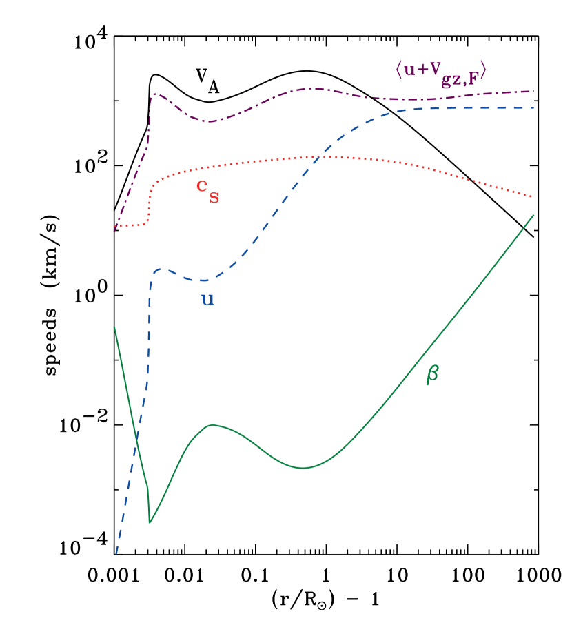
Figure 1.— Radial dependence of the Alfvén speed (black solid curve), solar wind outflow speed (blue dashed curve), one-fluid sound speed (red dotted curve), and the angle-averaged, intertial-frame group velocity of fast-mode waves (violet dot-dashed curve), all in units of km s^-1. Also shown is the dimensionless plasma $\beta$ parameter (green solid curve).

Figure 1 shows the radial dependence of a selection of the background plasma properties defined above. It also shows the dimensionless plasma beta parameter, which is usually defined as the ratio of gas pressure to magnetic pressure, with

$$\beta_{0}\,=\,\frac{P_{\rm gas}}{P_{\rm mag}}\,=\,\frac{2}{\gamma}\left(\frac{c_{s}}{V_{\rm A}}\right)^{2}\,\,.$$ (1)

However, we will often use a simpler dimensionless parameter $\beta$ given by

$$\beta\,=\,\left(\frac{c_{s}}{V_{\rm A}}\right)^{2}\,=\,\frac{\gamma\beta_{0}}{2}\,\,,$$ (2)

where $\beta$ and $\beta_{0}$ differ only by a factor of 1.2 when $\gamma=5/3$. The range of heights shown in Figure 1 extends down into the solar chromosphere, but the wave models discussed below start at a lower boundary condition in the low corona; i.e., they specify the wave and turbulence properties only for $z\geq 0.01\,R_{\odot}$.

2.2. Linear Properties of MHD Waves

In this section we briefly summarize the dispersion properties of linear MHD waves (i.e., phase and group speeds for the Alfvén mode and the fast and slow magnetosonic modes) and the partitioning between fluctuations in kinetic, magnetic, and thermal energy. In Sections 2.3–2.4 we assume that all three types of MHD waves are present, and we vary their relative strengths arbitrarily in order to match the observations.

The phase speed $V_{\rm ph}=\omega/k$ is defined in terms of the frequency $\omega$ and the magnitude of the wavenumber $k$. In general, $V_{\rm ph}$ is a function of the Alfvén speed, the sound speed, and the angle $\theta$ between the background field direction and the wavevector ${\bf k}$. We follow the standard convention of defining a Cartesian coordinate system with the background magnetic field along the $z$ axis and the ${\bf k}$ vector having components only in the $x$-$z$ plane. Also, for now we express $\omega$ and ${\bf k}$ in the frame comoving with the solar wind. For Alfvén waves,

$$V_{\rm ph}^{2}\,=\,V_{\rm A}^{2}\cos^{2}\theta$$ (3)

and for the magnetosonic modes,

$$V_{\rm ph}^{2}\,=\,\frac{V_{\rm A}^{2}+c_{s}^{2}}{2}\left(1\pm\Sigma\right)$$ (4)

applies with the upper sign corresponding to the fast mode and the lower sign corresponding to the slow mode, and with

$$\Sigma\,=\,\sqrt{1-\sigma\cos^{2}\theta}\,\,,\,\,\,\,\sigma\,=\,\frac{4\beta}{(1+\beta)^{2}}$$ (5)

(see, e.g., Whang, 1997; Goedbloed & Poedts, 2004). In Section 2.3 we also need to know the component of an MHD wave’s group velocity in the direction parallel to the background magnetic field. We call this quantity $V_{\rm gz}$, and for the Alfvén mode it is identically equal to $V_{\rm A}$ no matter the value of $\theta$. For the fast and slow modes,

$$V_{\rm gz}\,=\,V_{\rm ph}\cos\theta\left(1\mp\frac{\sigma\sin^{2}\theta}{2\Sigma\,(1\pm\Sigma)}\right)\,\,.$$ (6)

MHD waves excite oscillations in the plasma parameters. We denote the root-mean-square (rms) fluctuation amplitudes in velocity as $v_{x},v_{y},v_{z}$, in magnetic field as $B_{x},B_{y},B_{z}$, and in density as $\delta\rho$. We ignore fluctuations in the electric field because their contribution to the total energy density tends to be negligible when $V_{\rm A}\ll c$. The kinetic, magnetic, and thermal energy densities associated with each type of fluctuation are given as

$$K_{i}=\frac{\rho_{0}v_{i}^{2}}{2}\,\,,\,\,\,\,M_{i}=\frac{B_{i}^{2}}{8\pi}\,\,,\,\,\,\,\Theta=\beta\frac{B_{0}^{2}}{8\pi}\left(\frac{\delta\rho}{\rho_{0}}\right)^{2}$$ (7)

respectively, with $i=x,y,z$. For linear Alfvén waves, the total energy density $U_{\rm A}$ is divided equally between transverse kinetic and magnetic fluctuations along the $y$ axis, with $U_{\rm A}=K_{y}+M_{y}$ and

$$\frac{K_{y}}{U_{\rm A}}\,=\,\frac{M_{y}}{U_{\rm A}}\,=\,\frac{1}{2}\,\,.$$ (8)

For fast and slow mode waves,

$$U_{\rm F,S}\,=\,K_{x}+K_{z}+M_{x}+M_{z}+\Theta$$ (9)

and we follow Whang (1997) in expressing the partition fractions as follows,

$$\frac{K_{x}}{U_{\rm F,S}}=f_{n}\sin^{2}\theta+f_{t}\cos^{2}\theta\,,\,\,\frac{K_{z}}{U_{\rm F,S}}=f_{n}\cos^{2}\theta+f_{t}\sin^{2}\theta$$ (10)

$$f_{n}\,=\,\frac{V_{\rm ph}^{2}(V_{\rm ph}^{2}-V_{\rm A}^{2})}{c_{s}^{2}\Delta}\,\,,\,\,\,\,f_{t}\,=\,\frac{V_{\rm A}^{2}(V_{\rm ph}^{2}-c_{s}^{2})\cos^{2}\theta}{V_{\rm ph}^{2}\Delta}$$ (11)

$$\frac{M_{x}}{U_{\rm F,S}}\,=\,\frac{(V_{\rm ph}^{2}-c_{s}^{2})\cos^{2}\theta}{\Delta}\,\,,\,\,\,\,\frac{M_{z}}{U_{\rm F,S}}\,=\,\frac{(V_{\rm ph}^{2}-c_{s}^{2})\sin^{2}\theta}{\Delta}$$ (12)

$$\frac{\Theta}{U_{\rm F,S}}\,=\,\frac{V_{\rm ph}^{2}-V_{\rm A}^{2}}{\Delta}$$ (13)

where $\Delta=4V_{\rm ph}^{2}-2V_{\rm A}^{2}-2c_{s}^{2}$. The fast and slow velocity fluctuations ($K_{x}+K_{z}$) always occupy exactly half of the total energy density, and the combination of magnetic and thermal fluctuations ($M_{x}+M_{z}+\Theta$) take up the other half.

The energy partition fractions given above are familiar components of plasma physics and MHD textbooks (e.g., Stix, 1992; Goedbloed & Poedts, 2004). However, it is difficult to see intuitively how these fractions vary throughout the heliosphere from Equations (10)–(13) alone. Thus, in Figure 2 we provide a schematic illustration of the energy partitioning for fast-mode waves. The three columns indicate the variation from low ($\beta\ll 1$) to medium ($\beta=1$) and high ($\beta\gg 1$) beta plasmas. The three rows show the results for purely parallel propagation ($\theta=0$), an isotropic distribution of wavenumber vectors (see below), and purely perpendicular propagation ($\theta=\pi/2$). In general, all five terms on the right-hand side of of Equation (9) are nonzero, but fractions less than $\sim$1% are not shown in Figure 2. This diagram can be transformed to show the properties of slow-mode waves by replacing $\beta$ with $1/\beta$ and interchanging the $x$ and $z$ subscripts with one another.

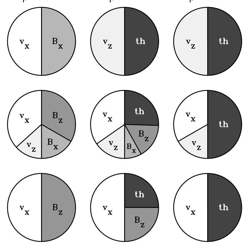
Figure 2.— Illustration of how fast-mode MHD waves divide their total fluctuation energy into kinetic, magnetic, and thermal energy in various regimes: wavevectors parallel to ${\bf B}_{0}$ (top row), an isotropic distribution of wavevectors (middle row), wavevectors perpendicular to ${\bf B}_{0}$ (bottom row); $\beta\ll 1$ (left column), $\beta=1$ (middle column), and $\beta\gg 1$ (right column). Plotted areas are proportional to the partition fractions given in Equations (10)–(13). Kinetic energy fractions are denoted by $v_{x}$ and $v_{z}$, magnetic energy fractions are denoted by $B_{x}$ and $B_{z}$, and the thermal energy fraction is denoted by ‘th’.

2.3. Radial Transport Equations

In order to determine how the total energy density of a given wave mode evolves with heliocentric distance, we solve equations of wave action conservation that contain multiple sources of wave damping. There have been many discussions of energy conservation for both pure acoustic waves and incompressible Alfvén waves (e.g., Dewar, 1970; Isenberg & Hollweg, 1982; Velli, 1993; Tu & Marsch, 1995; Verdini & Velli, 2007; Sokolov et al., 2009), but general derivations that can also be applied to fast and slow mode waves (for arbitrary $\theta$) are less frequently seen. We utilize the results of Jacques (1977) to write the damped wave action conservation equation as

$$\frac{\partial}{\partial t}\left(\frac{U_{m}}{\Omega}\right)+\frac{1}{A_{0}}\frac{\partial}{\partial r}\left(\frac{\langle u_{0}+V_{{\rm gz,}m}\rangle A_{0}U_{m}}{\Omega}\right)\,=\,-\frac{Q_{m}}{\Omega}$$ (14)

where the subscript $m$ can be replaced by A, F, or S for the relevant mode, $A_{0}$ is the cross sectional area of the flux tube (i.e., $A_{0}\propto 1/B_{0}$), and $Q_{m}$ is the total dissipation rate for the mode in question. The dimensionless factor that takes account of the “stretching” effect of wavelengths in an accelerating reference frame is

$$\Omega\,=\,\left\langle\frac{V_{{\rm ph,}m}}{u_{0}\cos\theta+V_{{\rm ph,}m}}\right\rangle$$ (15)

and the angle brackets denote a weighted average over all angles,

$$\langle f\rangle\,=\,\frac{\int d\theta\,\sin\theta\,f(\theta)}{\int d\theta\,\sin\theta}\,\,,$$ (16)

where here we consider outward propagating waves with $0<\theta<\pi/2$. The factor of $\cos\theta$ in Equation (15) comes from the difference between the wave frequency in the Sun’s reference frame ($\omega_{0}$) and the comoving-frame frequency ($\omega=\omega_{0}-{\bf k}\cdot{\bf u}_{0}$) that appears in the definition of the wave action; see Section III of Jacques (1977). Equation (14) implicitly assumes that $\omega_{0}$ remains constant, but it does not require the specification of any given value of $\omega_{0}$.

Our use of weighted averages over $\theta$ is derived from the assumption that wave power is distributed isotropically in three-dimensional ${\bf k}$ space. In Appendix A we discuss the motivations for assuming such an isotropic distribution of wavenumber vectors (specifically for the fast-mode waves). For Alfvén waves, this assumption has no impact on solving Equation (14), since the arguments of both angle-bracketed quantities given above are independent of $\theta$ (see also Hollweg, 1974). Thus, one obtains the same result for Alfvén waves whether one assumes a single value of $\theta$ or the isotropic distribution. For fast and slow mode MHD waves, some quantities depend strongly on $\theta$ and others do not. For example, slow-mode waves in low-beta plasmas have values of the angle-dependent quantity $u_{0}+V_{{\rm gz,}m}$ that are always nearly equal to $u_{0}+c_{s}$. Figure 1 shows the radial dependence of $\langle u_{0}+V_{\rm gz,F}\rangle$ for the isotropic distribution of fast-mode waves.

We solve Equation (14) for the energy densities of the three MHD modes ($U_{\rm A}$, $U_{\rm F}$, $U_{\rm S}$), and we compute the dispersion and energy partition properties of all three wave types as given in Section 2.2. At this stage, we neglect couplings between multiple modes and other nonlinear effects. This is an approximation that is likely to break down wherever the wave amplitudes become large (e.g., Chin & Wentzel, 1972; Wentzel, 1974; Goldstein, 1978; Lacombe & Mangeney, 1980; Poedts et al., 1998; Vasquez & Hollweg, 1999; Del Zanna et al., 2001; Gogoberidze et al., 2007). In Section 4 we discuss the likelihood of rapid coupling between the high-wavenumber tails of the Alfvén and fast-mode power spectra. However, we continue to assume that the total energy densities are given by the solution of the individual transport equations.

To specify the dissipation rates $Q_{m}$, we include both linear collisional effects (e.g., viscosity, thermal conductivity, and electrical resistivity) for all three modes and nonlinear turbulent damping for the Alfvén and fast mode. Thus, we use

$$Q_{\rm A}=\tilde{Q}_{\rm A}+2\gamma_{\rm A}U_{\rm A}\,\,,\,\,\,\,Q_{\rm F}=\tilde{Q}_{\rm F}+2\gamma_{\rm F}U_{\rm F}\,\,,\,\,\,\,Q_{\rm S}=2\gamma_{\rm S}U_{\rm S}\,\,.$$ (17)

We give the amplitude damping rates $\gamma_{m}$, which include an approximation for the transition from strongly collisional to collisionless regimes, in Appendix B. The turbulent damping rates $\tilde{Q}_{\rm A}$ and $\tilde{Q}_{\rm F}$ are described in more detail below. In general, these rates depend on the parallel and perpendicular components of the wavenumber $(k_{\parallel},k_{\perp})$. For the purposes of evaluating these rates in the global wave transport equations, we assumed that $k_{\perp}=1/\lambda_{\perp}$ for all three modes, where $\lambda_{\perp}$ is the turbulent correlation length described below. For the fast and slow modes, our assumption of an isotropic distribution of wavenumbers is consistent with also assuming $k_{\parallel}=k_{\perp}$. For the Alfvén mode, we found that $\gamma_{\rm A}$ never depended on the assumed value of $k_{\parallel}$ at all, but for completeness we used the critical balance condition (introduced in Appendix A) to specify $k_{\parallel}$.

We adopt phenomenological forms for the turbulent dissipation rates that are equivalent to the total energy fluxes that cascade from large to small scales. Thus, $\tilde{Q}_{\rm A}$ and $\tilde{Q}_{\rm F}$ are constrained only by the properties of fluctuations at the largest scales, and they do not specify the exact kinetic means of dissipation once the energy reaches the smallest scales (but see, however, Section 5). Dimensionally, these are similar to the rate of cascading energy flux derived by von Kármán & Howarth (1938) for isotropic hydrodynamic turbulence. For the nonlinear dissipation of Alfvénic fluctuations, we use

$$\tilde{Q}_{\rm A}\,=\,\rho_{0}\,\tilde{\alpha}_{\rm A}{\cal E}_{\rm turb}\,\frac{Z_{-}^{2}Z_{+}+Z_{+}^{2}Z_{-}}{4\lambda_{\perp}}$$ (18)

(see also Hossain et al., 1995; Zhou & Matthaeus, 1990a; Matthaeus et al., 1999; Dmitruk et al., 2001, 2002; Breech et al., 2008). For the fast-mode waves, we use

$$\tilde{Q}_{\rm F}\,=\,\rho_{0}\,\tilde{\alpha}_{\rm F}\,\frac{(v_{x}^{2}+v_{z}^{2})^{2}}{V_{\rm A}\lambda_{\perp}}$$ (19)

where the quantity $(v_{x}^{2}+v_{z}^{2})$ collects together the total kinetic energy in fast-mode velocity fluctuations (Chandran, 2005; Suzuki et al., 2007). Many of the terms introduced in Equations (18)–(19) are defined throughout the remainder of this subsection.

Equation (18) depends on the magnitudes of the Elsasser (1950) variables, $Z_{\pm}=v_{y}\pm B_{y}/(4\pi\rho_{0})^{1/2}$, which specify the power in outward ($Z_{-}$) and inward ($Z_{+}$) propagating Alfvénic fluctuations. Alfvénic turbulent heating occurs only when there is energy in both modes. In practice we compute an effective reflection coefficient ${\cal R}=|Z_{+}|/|Z_{-}|$ whose magnitude is always less than unity, and thus we express the Elsasser variables in terms of the Alfvénic energy density as

$$Z_{-}\,=\,\sqrt{\frac{4U_{\rm A}}{\rho_{0}(1+{\cal R}^{2})}}\,\,,\,\,\,\,Z_{+}\,=\,{\cal R}Z_{-}\,\,.$$ (20)

An accurate solution for $Z_{\pm}$ requires the integration of non-WKB equations of Alfvén wave reflection (e.g., Heinemann & Olbert, 1980; Verdini & Velli, 2007). However, our assumption that the total power $U_{\rm A}$ varies in accord with straightforward wave action conservation has been shown to be reasonable, even in environments where ${\cal R}$ is not small such as the chromosphere (van Ballegooijen et al., 2011) and interplanetary space (Zank et al., 1996; Cranmer & van Ballegooijen, 2005).

We estimate the reflection coefficient ${\cal R}$ using a modification of the low-frequency approximation of Chandran & Hollweg (2009). Specifically, we examine the magnitudes of terms in the transport equation for the inward Elsasser variable,

$$\frac{\partial Z_{+}}{\partial t}+(u_{0}-V_{\rm A})\frac{\partial Z_{+}}{\partial r}=(u_{0}+V_{\rm A})\left(\frac{Z_{+}}{4H_{\rm D}}+\frac{Z_{-}}{2H_{\rm A}}\right)-\frac{Z_{+}Z_{-}}{2\lambda_{\perp}}$$ (21)

where

$$H_{\rm A}=\frac{V_{\rm A}}{\partial V_{\rm A}/\partial r}\,\,,\,\,\,\,H_{\rm D}=\frac{\rho_{0}}{\partial\rho_{0}/\partial r}\,\,.$$ (22)

Chandran & Hollweg (2009) neglected both terms on the left-hand side of Equation (21) as well as the term containing $H_{\rm D}$, and thus were able to solve for $Z_{+}$ straightforwardly. However, in cases of strong reflection, the term containing $H_{\rm D}$ may have a magnitude comparable to the other dominant terms. Thus, we keep all three terms on the right-hand side and solve for

$${\cal R}\,\approx\,\frac{2h/|H_{\rm A}|}{1+(h/|H_{\rm D}|)}$$ (23)

where

$$h\,=\,\frac{\lambda_{\perp}(u_{0}+V_{\rm A})}{2Z_{-}}\,\,.$$ (24)

Equation (22) of Chandran & Hollweg (2009) is recovered in the limit of $h\ll|H_{\rm D}|$, with ${\cal R}\approx 2h/|H_{\rm A}|$. In the case of purely linear reflection, Cranmer (2010) found that the most accurate local estimates for ${\cal R}$ were obtained when $H_{\rm A}$ was replaced with the positive-definite quantity

$$\tilde{H}_{\rm A}\,=\,V_{\rm A}t_{\rm ref}\,=\,(r+R_{\odot})\left(1-\frac{R_{\odot}}{r}\right)\,\,.$$ (25)

We used $\tilde{H}_{\rm A}$ instead of $H_{\rm A}$ in Equations (23)–(24) to compute ${\cal R}$.

The definitions of the turbulent dissipation rates contain the perpendicular length scale $\lambda_{\perp}$, which is an effective transverse correlation length of the turbulence for the largest “outer scale” eddies. For simplicity we use the same correlation length for both the Alfvénic and fast-mode fluctuations, but this may not be universally valid (e.g., Suzuki et al., 2007). In previous papers we assumed that $\lambda_{\perp}$ scales with the transverse width of the magnetic flux tube; i.e., that $\lambda_{\perp}\propto B_{0}^{-1/2}$ (Hollweg, 1986). Here we describe the evolution of the transverse correlation length $\lambda_{\perp}$ with the following transport equation,

$$\frac{\partial\lambda_{\perp}}{\partial r}\,=\,\frac{\lambda_{\perp}}{2A_{0}}\frac{\partial A_{0}}{\partial r}+\frac{\tilde{\beta}_{\rm A}}{u_{0}+V_{\rm A}}\left(\frac{Z_{-}^{2}Z_{+}+Z_{+}^{2}Z_{-}}{Z_{-}^{2}+Z_{+}^{2}}\right)\,\,,$$ (26)

where $\tilde{\beta}_{\rm A}$ is a dimensionless constant that is often assumed to be equal to $\tilde{\alpha}_{\rm A}/2$ (e.g., Hossain et al., 1995). The first term on the right-hand side of Equation (26) drives the correlation length to expand linearly with the perpendicular flux-tube cross section (Hollweg, 1986). The second term takes account of the nonlinear coupling between the fluctuations and the background plasma properties. It is given in a form suggested initially by Matthaeus et al. (1994) and later generalized to nonzero cross-helicity turbulence by Breech et al. (2008) and others. Our transport equation attempts to bridge together the effects of the two terms. In the lower solar atmosphere (between the photosphere and the chosen lower boundary of 0.01 $R_{\odot}$ for the wave transport models) we assumed that the first term in Equation (26) is dominant, and thus $\lambda_{\perp}\propto A_{0}^{1/2}$.

The turbulent dissipation rates also depend on dimensionless Kolmogorov-type constants $\tilde{\alpha}_{\rm A}$ and $\tilde{\alpha}_{\rm F}$ that are often assumed to have values of order unity. For example, Hossain et al. (1995) and Breech et al. (2009) found that $\tilde{\alpha}_{\rm A}\approx 0.5$ gives rise to dissipation rates that agree well with both numerical simulations and heliospheric observations. In our case, we used this value as a starting point, but we also varied $\tilde{\alpha}_{\rm A}$ as a free parameter in order to produce the best match to the well-constrained Alfvénic fluctuations. On the other hand, the properties of heliospheric fast-mode turbulence are not known nearly as well as the Alfvén-wave turbulence. We thus relied on the independent wave-kinetic simulations of Pongkitiwanichakul & Chandran (2012) to fix $\tilde{\alpha}_{\rm F}$ at a value of 2.3.

The Alfvénic cascade rate contains an efficiency factor ${\cal E}_{\rm turb}$ that attempts to account for regions where the turbulent cascade may not have time to develop before the fluctuations are carried away by the wind. Cranmer et al. (2007) estimated this efficiency factor to scale as

$${\cal E}_{\rm turb}\,=\,\frac{1}{1+(t_{\rm eddy}/t_{\rm ref})}\,\,,$$ (27)

where the two timescales above are $t_{\rm eddy}$, a nonlinear eddy cascade time, and $t_{\rm ref}$, a timescale for large-scale Alfvén wave reflection (see also Dmitruk & Matthaeus, 2003; Oughton et al., 2006). The reflection time is often defined as $t_{\rm ref}=1/|\nabla\cdot{\bf V}_{A}|$, but we solved Equation (25) for $t_{\rm ref}$ in order to remain consistent with the adopted model for ${\cal R}$. The eddy cascade time is given by

$$t_{\rm eddy}\,=\,\frac{\lambda_{\perp}\sqrt{3\pi}}{(1+M_{\rm A})\,v_{y}}\,\,,$$ (28)

where the Alfvén Mach number $M_{\rm A}=u_{0}/V_{\rm A}$ and the numerical factor of $3\pi$ comes from the normalization of an assumed shape of the turbulence spectrum (see Appendix C of Cranmer & van Ballegooijen, 2005). The two limiting cases of ${\cal E}_{\rm turb}\ll 1$ and ${\cal E}_{\rm turb}\approx 1$ are roughly equivalent to the “weak” and “strong” cascade phenomenologies discussed in Section 3, but they are not precisely the same.

2.4. Representative Solutions

We solved the transport equations given in Section 2.3 by numerically integrating upwards from a specified set of lower boundary conditions at $z=0.01\,R_{\odot}$ and assuming time-steady conditions (i.e., $\partial U_{m}/\partial t=0$). We used a logarithmic grid of 500 radial zones in $z$ that expands out to a maximum distance of $860\,R_{\odot}\approx 4$ AU. The transport equations were solved with straightforward first-order Euler steps. The values of the Elsasser variables $Z_{\pm}$ in each zone were determined by iteration, since Equations (20) and (23) do not give a simple closed-form solution for $Z_{+}$ and $Z_{-}$ by themselves.

There are a number of free parameters in this model whose values were not easily obtained from either theoretical calculations or observations. In addition to the lower boundary conditions on the wave energy densities $U_{\rm A}$, $U_{\rm F}$, and $U_{\rm S}$, there is also the lower boundary condition on the correlation length $\lambda_{\perp}$ and the values of the two von Kármán constants $\tilde{\alpha}_{\rm A}$ and $\tilde{\beta}_{\rm A}$. Initially, we varied these six parameters randomly in order to build up a large Monte Carlo ensemble of trial solutions. For each model, we synthesized the radial variation of observable plasma fluctuations such as the root mean squared (rms) parallel and perpendicular fluctuation speeds,

$$v_{\parallel}\,=\,v_{z}\,\,,\,\,\,\,\,\,\,v_{\perp}\,=\,(v_{x}^{2}+v_{y}^{2})^{1/2}\,\,,$$ (29)

the Elsasser variables $Z_{\pm}$, and the rms fractional density fluctuation amplitude $\delta\rho/\rho_{0}$. The velocity amplitudes $v_{\parallel}$ and $v_{\perp}$ contain contributions from all three MHD wave types. In nearly all models produced here, $v_{\parallel}$ is dominated by the fast mode and $v_{\perp}$ is dominated by the Alfvén mode. Observations of these quantities are discussed below.

Table 1Standard Model Parameters for Coronal Hole MHD Wave Transport

Parameter	Value
$\tilde{\alpha}_{\rm A}$	0.60
$\tilde{\beta}_{\rm A}$	0.31
$\tilde{\alpha}_{\rm F}$	2.3
$(U_{\rm A}/\rho_{0})^{1/2}$ (at $z=0.01\,R_{\odot}$)	29.0 km s-1
$(U_{\rm F}/\rho_{0})^{1/2}$ (at $z=0.01\,R_{\odot}$)	24.3 km s-1
$(U_{\rm S}/\rho_{0})^{1/2}$ (at $z=0.01\,R_{\odot}$)	9.17 km s-1
$\lambda_{\perp}$ (at photosphere)	120 km

There was no single set of parameter values that gave rise to perfect agreement between all of the synthesized and observed fluctuation quantities. This is not surprising, since the models are certainly incomplete and there are significant uncertainties in the observations and their interpretation. Also, even though we aimed to restrict ourselves to measurements made in “quiet” high-latitude fast wind streams, sometimes only low-latitude data were available. Thus, in Table 1 we give a set of optimized parameters that were chosen because they produce adequate agreement with the full set of observed quantities. There were other combinations of the six parameters that gave better agreement on any single observation, but in most of these cases the agreement became worse for other observations. Although the ratio of the two von Kármán constants $\tilde{\alpha}_{\rm A}/\tilde{\beta}_{\rm A}$ was allowed to vary freely, the optimal value was nonetheless found to be close to the commonly used value of 2 (Hossain et al., 1995). The best photospheric value of $\lambda_{\perp}\approx 120$ km is intermediate between the values of 75 km (Cranmer et al., 2007) and 300 km (Cranmer & van Ballegooijen, 2005) found from earlier models.

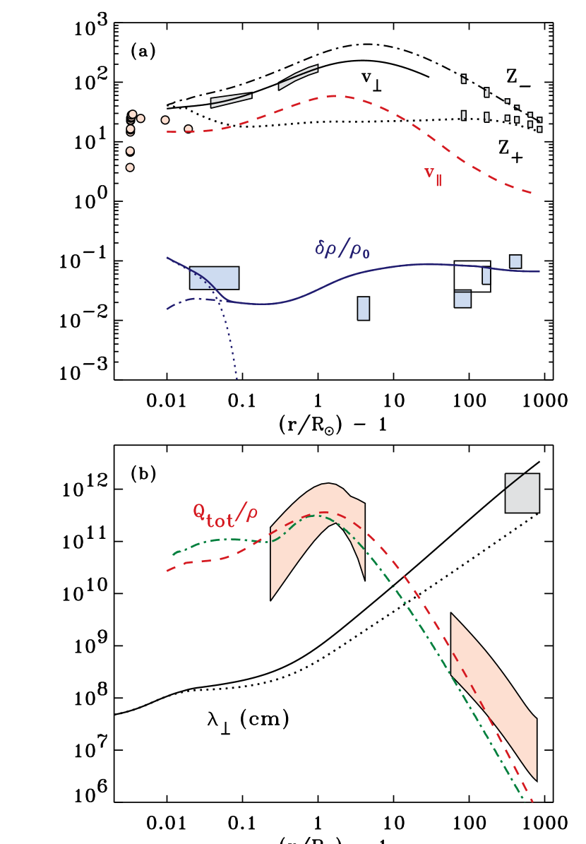
Figure 3.— (a) Model values for $v_{\perp}$ (black solid curve), $Z_{-}$ (black dot-dashed curve), and $Z_{+}$ (black dotted curve) compared with measurements (gray boxes). Model values for $v_{\parallel}$ (red dashed curve) compared with measurements (light red circles). Velocities are plotted in units of km s^-1; see Equation (29). Total density amplitude $\delta\rho/\rho_{0}$ (blue solid curve) is shown with its components from fast-mode (blue dot-dashed curve) and slow-mode (blue dotted curve) waves, and compared with observations (light blue regions and rectangles). (b) Modeled total heating rate $Q_{\rm tot}/\rho_{0}$ (red dashed curve) compared with empirical constraints (light red regions) and the total heating rate from Cranmer et al. (2007) (green dot-dashed curve), all in erg s^-1 g^-1. Standard model value for $\lambda_{\perp}$ (solid black curve) compared with earlier assumption $\lambda_{\perp}\propto B_{0}^{-1/2}$ (black dotted curve) and with in situ estimates (gray region), shown in units of cm. See text for data sources.

Figure 3 shows the comparison between synthesized and observed fluctuation quantities for the model parameters given in Table 1. The observational constraints on $v_{\perp}$ at $z\lesssim 0.1\,R_{\odot}$ are a combination of the off-limb nonthermal emission line widths given by Banerjee et al. (1998) and Landi & Cranmer (2009). The observations shown between 0.3 and 1 $R_{\odot}$ are from Esser et al. (1999). At larger heights, $v_{\perp}$ becomes approximately equal to $Z_{-}/2$, so we truncate the $v_{\perp}$ curve in favor of showing the radial dependence of $Z_{+}$ and $Z_{-}$ more clearly. The latter are compared directly with high-speed wind data from Helios and Ulysses (Bavassano et al., 2000). Observations of longitudinal velocity fluctuations are more difficult to find, and we show only the on-disk nonthermal line width velocities of Chae et al. (1998) as a way to compare with the modeled values of $v_{\parallel}$.

Figure 3(a) shows how the modeled density fluctuation amplitude $\delta\rho/\rho_{0}$ is dominated by slow-mode waves in the low corona ($z\lesssim 0.1\,R_{\odot}$) and by fast-mode waves in the extended corona and solar wind ($z\gtrsim 1\,R_{\odot}$). The low-corona observations are drawn as an approximate boundary region around the polar plume data given by Ofman et al. (1999). The intermediate data point at $z=4\,R_{\odot}$ is an empirical value of $\delta\rho/\rho_{0}$ estimated from radio sounding data (Coles & Harmon, 1989; Spangler, 2002; Harmon & Coles, 2005; Chandran et al., 2009), but it is still unclear what fraction of the measured density fluctuations are due to anything even close to ideal MHD waves. At larger distances, we show approximate ranges of density fluctuations as reported by Marsch & Tu (1990) (blue rectangles at $z<200\,R_{\odot}$), Tu & Marsch (1994) (open rectangle), and Issautier et al. (1998) (blue rectangle at $z>300\,R_{\odot}$).

Figure 3(b) compares the result of solving Equation (26) for $\lambda_{\perp}$ with the simpler approximation of $\lambda_{\perp}\propto B_{0}^{-1/2}$. The plot also shows fast-wind estimates of $\lambda_{\perp}$ between 1.4 and 5 AU from Ulysses (Breech et al., 2008). Figure 3(b) also compares the total heating rate $Q_{\rm tot}=Q_{\rm A}+Q_{\rm F}+Q_{\rm S}$ with observational constraints and with the modeled coronal heating rate from Cranmer et al. (2007). The shaded area between 0.2 and 5 $R_{\odot}$ is an envelope surrounding a collection of empirical and theoretical heating curves from Wang (1994), Hansteen & Leer (1995), and Allen et al. (1998). These rates illustrate what is needed to produce the observed coronal heating and solar wind acceleration. The area shown at larger distances ($z>60\,R_{\odot}$) is a representation of the range of total (proton and electron) empirical heating rates estimated by Cranmer et al. (2009). Note that the turbulent heating rates $\tilde{Q}_{\rm A}$ and $\tilde{Q}_{\rm F}$ dominate the total heating rate, with approximately 70% of the total coming from $\tilde{Q}_{\rm A}$ and 20% from $\tilde{Q}_{\rm F}$. Less than 10% of $Q_{\rm tot}$ comes from the linear damping terms.

There are additional measurement techniques that may be used to further constrain the model parameters, and in future work we will incorporate as many of these as possible. For example, Hollweg et al. (2010) argued that radio measurements of Faraday rotation fluctuations may put unique empirical constraints on the value of $\lambda_{\perp}$ in the corona. Also, Sahraoui et al. (2010) used multi-spacecraft data to tease out new details of the wavenumber anisotropy of MHD fluctuations, which may lead to better limits on, e.g., $v_{\parallel}/v_{\perp}$ in the heliosphere. Unfortunately, the vast majority of these measurements have been made for the slow solar wind and not the much less structured fast wind associated with polar coronal holes. Nearer to the Sun, Kitagawa et al. (2010) used the dispersive and energy partition properties of thin-tube MHD waves to diagnose the presence and strengths of various modes in active regions. These techniques may be useful in open-field regions as well.

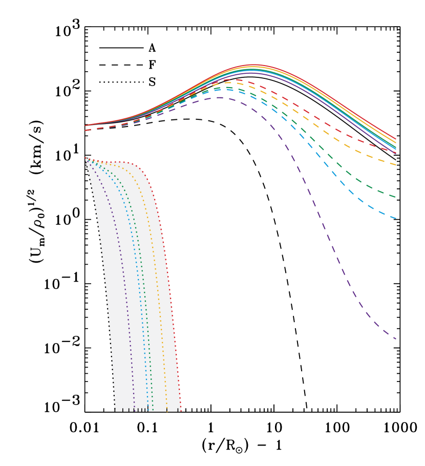
Figure 4.— Radial dependence of MHD wave energy densities per unit mass, for a range of photospheric boundary conditions on on $\lambda_{\perp}$. From bottom to top in each set of curves, the values are: 30 km (black), 60 km (dark blue), 100 km (cyan), 120 km (green), 200 km (orange), and 300 km (red). Different line styles denote Alfvén waves (solid curves), fast-mode waves (dashed curves), and slow-mode waves (dotted curves surrounded by gray background).

Although we did not include any explicit multi-mode coupling in the transport equations of Section 2.3, there is some feedback between the modes. For example, the correlation length $\lambda_{\perp}$ is used in both the Alfvénic and fast-mode turbulent heating expressions, and it is also used to set the wavenumbers $k_{\parallel}$ and $k_{\perp}$ in the linear dissipation rates $\gamma_{m}$. Thus, the choice of the lower boundary condition on $\lambda_{\perp}$ can have a significant impact on the radial evolution of all three wave types. Figure 4 illustrates this by varying the photospheric value of $\lambda_{\perp}$ between 30 and 300 km and using the other standard parameters from Table 1. The integrated energy densities are plotted in velocity units as $(U_{m}/\rho_{0})^{1/2}$. The power in the Alfvén waves changes by only a small amount because the damping is never a strong contributor to the $U_{\rm A}$ transport equation. However, damping is a major effect for the fast and slow modes, and thus small changes in the damping rate’s normalization can have large relative impacts on the resulting energy densities.

Figure 4 shows that, no matter the choice of normalization for $\lambda_{\perp}$, it seems unlikely for the slow-mode waves to have significantly large amplitudes anywhere but in the lowest few tenths of a solar radius. This appears to be consistent with models of slow-mode shock formation and dissipation in polar plumes (Cuntz & Suess, 2001). Therefore, in the remainder of this paper, our models of turbulence in the fast solar wind ignore the slow-mode waves altogether. We also note that Figure 4 suggests that the actual fast-mode wave properties in the high-speed solar wind may be more highly variable than the Alfvén wave properties. Our use of a “standard” model for the fast-mode waves (using the parameters given in Table 1) is thus presented as an example case and not a definitive prediction.

3. MHD Turbulent Cascade

In this section we begin constructing a model of the wavenumber distribution of Alfvén and fast-mode fluctuation power at each radial distance. We make use of a general assumption of “scale separation;” i.e., we presume that the turbulence becomes fully developed on timescales short compared to the bulk solar wind outflow and the large-scale expansion of open flux tubes. This allows us to model the turbulence as spatially homogeneous in a small volume element with constant background plasma properties. This seems to be the general assumption made by the majority of MHD simulations of turbulence in the solar wind. Whether or not this approximation is valid, it is useful to begin studying the wavenumber dependence of the cascade in this manner.

3.1. Wavenumber Advection-Diffusion Equations

We model the MHD fluctuations as time-steady Fourier distributions of wave power in three-dimensional wavenumber space. Although additional information about the physics of turbulence can be found in more complex statistical measures of the system (e.g., higher-order structure functions), we limit ourselves to describing the power spectrum because that is the basic quantity needed to compute the quasilinear particle heating rates.

Because of the simplified flux-tube geometry discussed in Section 2.1, we assume the background magnetic field is parallel to the bulk flow velocity, and thus the system has only one preferred spatial direction (see, however, Narita et al., 2010). The random turbulent motions create a statistical equivalence between the $x$ and $y$ directions transverse to the background field, so that we can describe the power spectra as two-dimensional functions of $k_{\parallel}$ and $k_{\perp}$ only. By convention, we define the full three-dimensional power spectrum $E_{m}$ in effective velocity-squared units; i.e., when integrated over the full volume of wavenumber space, the spectrum gives the fluctuation energy density per unit mass, or

$$\frac{U_{m}}{\rho_{0}}\,=\,\int d^{3}{\bf k}\,\,E_{m}({\bf k})\,\,.$$ (30)

In Appendix A we review some of the basic physical processes that determine the shape of the spectrum for Alfvénic ($m=\mbox{A}$) and fast-mode ($m=\mbox{F}$) fluctuations.

We describe the driven turbulent cascade as a combination of advection and diffusion in wavenumber space. At first, it may appear that a smooth and continuous description of the spectral “spreading” of a cascade ignores too much of the inherently stochastic and nonlocal nature of turbulence. However, Chandrasekhar (1943) showed that such a model can be made to capture the essential statistics of a large ensemble of random-walk-like (i.e., Brownian) processes. Specific models of turbulent wavenumber transport using diffusion or advection equations include those of Pao (1965), Leith (1967), Tu et al. (1984), Tu (1988), Zhou & Matthaeus (1990b), Miller et al. (1996), Stawicki et al. (2001), Chandran (2008b), Matthaeus et al. (2009), Jiang et al. (2009), and Galtier & Buchlin (2010). For the cascade of Alfvénic fluctuations, we generally follow the approach taken by Cranmer & van Ballegooijen (2003). The general forms of these equations are given as

$$\frac{\partial E_{\rm A}}{\partial t}\,=\,\frac{1}{k_{\perp}}\frac{\partial}{\partial k_{\perp}}\left\{D_{{\rm A}\perp}\left[\frac{\alpha_{\perp}}{k_{\perp}}\frac{\partial}{\partial k_{\perp}}\left(k_{\perp}^{2}E_{\rm A}\right)-\mu_{\perp}E_{\rm A}\right]\right\}$$

$$+\,\,\alpha_{\parallel}\frac{\partial}{\partial k_{\parallel}}\left(D_{{\rm A}\parallel}\frac{\partial E_{\rm A}}{\partial k_{\parallel}}\right)+S_{\rm A}-2\gamma_{\rm A}E_{\rm A}+C_{\rm AF}$$ (31)

$$\frac{\partial E_{\rm F}}{\partial t}\,=\,\frac{\alpha_{\rm F}}{k^{2}}\frac{\partial}{\partial k}\left(k^{2}D_{\rm F}\frac{\partial E_{\rm F}}{\partial k}\right)+S_{\rm F}-2\gamma_{\rm F}E_{\rm F}-C_{\rm AF}$$ (32)

and the terms on the right-hand sides of Equations (31)–(32) are defined throughout the remainder of this subsection. The mode coupling term $C_{\rm AF}$ is described further in Section 4, and the dissipation rates $\gamma_{\rm A}$ and $\gamma_{\rm F}$ are described in Section 5.

The perpendicular Alfvénic cascade is described by the first term on the right-hand side of Equation (31), and we assume an arbitrary linear combination of advection and diffusion. Cranmer & van Ballegooijen (2003) found that many key properties of the turbulence do not depend on whether the cascade is modeled as advection, diffusion, or both, so we retain all terms for maximum generality. For both the parallel Alfvénic spectral transport and the isotropic fast-mode transport, a more standard diffusion coefficient is assumed. The dimensionless multipliers to the $E_{\rm A}$ diffusion coefficients are denoted $\alpha_{\perp}$ and $\alpha_{\parallel}$, to correspond roughly to $\tilde{\alpha}_{\rm A}$ in Equation (18), and the dimensionless multiplier for the wavenumber advection coefficient is denoted $\mu_{\perp}$.

For the Alfvénic cascade, the overall behavior of wavenumber transport in the perpendicular and parallel directions is specified by the diffusion-like coefficients

$$D_{{\rm A}\perp}\,=\,\frac{k_{\perp}^{2}}{\tau_{\rm A}}\,\,,\,\,\,\,D_{{\rm A}\parallel}\,=\,\left(\frac{v_{\perp}}{V_{\rm A}}\right)^{2}D_{{\rm A}\perp}$$ (33)

where $\tau_{\rm A}$ is the cascade timescale defined below, and $v_{\perp}$ is the $k_{\perp}$-dependent velocity response of the waves. Note that $D_{{\rm A}\parallel}$ is independent of $k_{\parallel}$, so it can be pulled out of the derivative in Equation (31). Cranmer & van Ballegooijen (2003) showed that the above form for the diffusion coefficients tends to reproduce the Goldreich & Sridhar (1995) critical balance, and Matthaeus et al. (2009) derived similar functional forms for the coefficients. When specifying the properties of the wavenumber cascade, we apply the scalings for “balanced” turbulence (i.e., zero cross helicity, or $Z_{+}=Z_{-}$), which is more straightforward to implement but is formally inconsistent with the large-scale transport model of Section 2.

For ideal MHD Alfvénic fluctuations, $v_{\perp}^{2}$ is equal to $b_{\perp}^{2}$, the latter representing the transverse magnetic variance spectrum divided by $4\pi\rho_{0}$ to convert it to units of velocity squared. Following the usual convention, the power spectrum $E_{\rm A}$ tracks the magnetic fluctuations, so the reduced spectra are defined formally as

$$b_{\perp}^{2}\,=\,k_{\perp}^{2}\int dk_{\parallel}\,E_{\rm A}\,\,,\,\,\,v_{\perp}^{2}\,=\,\phi b_{\perp}^{2}\,\,.$$ (34)

The dimensionless factor $\phi$ describes the departure from ideal MHD energy equipartition. For small values of $k_{\perp}$, we assume $\phi\approx 1$. However, as $k_{\perp}$ increases into the regime of kinetic Alfvén waves (KAWs), $\phi$ can become much larger than 1. Hollweg (1999) described how the main difference between $v_{\perp}$ and $b_{\perp}$ in the KAW regime comes from an enhanced response of the electron velocity distribution to the electric and magnetic fluctuations. For simplicity, we use an approximate analytic expression

$$\phi\,=\,\frac{\omega^{2}}{k_{\parallel}^{2}V_{\rm A}^{2}}\,\approx\,\frac{1+k_{\perp}^{2}\rho_{p}^{2}}{1+k_{\perp}^{2}\rho_{p}^{2}m_{e}/(\beta m_{p})}\,\,,$$ (35)

where $\rho_{p}=w_{p}/\Omega_{p}$ is the proton thermal gyroradius, with the proton most-probable speed given by $w_{p}=(2k_{\rm B}T_{p}/m_{p})^{1/2}$ and the proton cyclotron frequency by $\Omega_{p}=eB/m_{p}c$. Our term $\phi$ is equivalent to $\alpha^{2}$ as defined by Howes et al. (2008).

Inspired by Equation (A6), we define the Alfvénic spectral transport timescale as

$$\tau_{\rm A}\,=\,\frac{1+\chi_{0}}{k_{\perp}v_{\perp}}$$ (36)

where we chose to replace the general critical balance parameter $\chi$ by its value at the outer-scale parallel wavenumber $k_{0\parallel}$. Thus,

$$\chi_{0}\,=\,\frac{\omega_{0}}{k_{\perp}v_{\perp}}\,\approx\,\frac{k_{0\parallel}V_{\rm A}}{k_{\perp}b_{\perp}}\,\,,$$ (37)

and $\chi_{0}$ is the appropriate critical balance parameter to use when solving for the properties of the dominant low-frequency cascade. From Equation (35) we see that KAW outer-scale frequency $\omega_{0}\approx\phi^{1/2}k_{0\parallel}V_{\rm A}$, so that a factor of $\phi^{1/2}$ cancels out of both the numerator and denominator to give the final approximate expression above. The wavenumber $k_{0\parallel}$ specifies the spatial scale along the field at which energy is injected in the source term $S_{\rm A}$ (see below). Because $k_{0\parallel}$ is assumed to be constant (at a given heliocentric distance $r$), the parameters $\chi_{0}$ and $\tau_{\rm A}$ are both functions of $k_{\perp}$ and not $k_{\parallel}$. The above form for Equation (36) was motivated by the analysis of Zhou & Matthaeus (1990b), Chandran (2008b), and Howes et al. (2012), who described how the cascade and wavenumber anisotropy change when the system transitions from weak ($\chi_{0}\gg 1$) to strong ($\chi_{0}\ll 1$) turbulence.

As mentioned above, our expressions for $\tau_{\rm A}$, $D_{{\rm A}\perp}$, and $D_{{\rm A}\parallel}$ assume zero cross helicity (i.e., ${\cal R}=1$). There is still no agreement about how to generalize these terms when inefficient wave reflection gives rise to nonzero cross helicity. Lithwick et al. (2007) found that the cascade timescales for outward and inward wave modes are different from one another when ${\cal R}\neq 1$, but their parallel spatial scales are the same. However, Beresnyak & Lazarian (2008, 2009) found that $k_{\parallel}$ for the outward mode should be larger than $k_{\parallel}$ for the inward mode, and thus the Goldreich & Sridhar (1995) critical balance must be modified (see Equation (45) below). Chandran (2008b) outlined a method for setting up the advection-diffusion equations in the case of ${\cal R}\neq 1$, but we defer a full implementation of that approach to future work.

Putting aside the issue of imbalanced turbulence, the dominant perpendicular nature of the Alfvénic cascade allows us to define a reduced transport equation that follows the evolution of the spectrum as a function of $k_{\perp}$ only. If we ignore the mode coupling term $C_{\rm AF}$ for now, we can multiply Equation (31) by $k_{\perp}^{2}$ and integrate over $k_{\parallel}$ to obtain

$$\frac{\partial b_{\perp}^{2}}{\partial t}=k_{\perp}\frac{\partial}{\partial k_{\perp}}\left[\frac{1}{\tau_{\rm A}}\left(\alpha_{\perp}k_{\perp}\frac{\partial b_{\perp}^{2}}{\partial k_{\perp}}-\mu_{\perp}b_{\perp}^{2}\right)\right]+\tilde{S}_{\rm A}-2\tilde{\gamma}_{\rm A}b_{\perp}^{2}\,.$$ (38)

This is essentially the same as Equation (11) of Cranmer & van Ballegooijen (2003). The reduced source term $\tilde{S}_{\rm A}$ and dissipation rate $\tilde{\gamma}_{\rm A}$ are defined similarly to the corresponding terms in Equation (31), but they are weighted toward the low-$k_{\parallel}$ regions of wavenumber space that are “filled” by the cascade. In Appendices C.1–C.3 we derive analytic solutions for the time-steady Alfvén-wave power spectrum in various limiting cases.

The cascade of fast-mode waves, described by Equation (32), appears to be conceptually simpler than the strongly anisotropic Alfvén-wave cascade. The diffusion coefficient is given by $D_{\rm F}=k^{2}/\tau_{\rm F}$, where $\tau_{\rm F}$ is related to the IK-like cascade time given by Equation (A2) with $p=1$. There is increasing evidence (e.g., Markovskii et al., 2010) that a fast-mode cascade is more rapid in the directions perpendicular to the field than along the field. However, the cascade does appear to proceed outward “radially” in the direction of increasing $k$. Thus, it makes the most sense to use an isotropic diffusion formalism as in Equation (32), but scale the magnitude of the diffusion timescale with $\theta$. Following the weak turbulence model of Chandran (2005), we adopt

$$\tau_{\rm F}\,=\,\frac{V_{\rm A}}{kv_{k}^{2}\sin\theta}\,\,,$$ (39)

which implies that

$$D_{\rm F}\,=\,\frac{k^{3}v_{k}^{2}\sin\theta}{V_{\rm A}}\,=\,\frac{4\pi k^{6}E_{\rm F}\sin\theta}{V_{\rm A}}\,\,.$$ (40)

Chandran (2005) showed that the $\sin\theta$ dependence in the denominator of $\tau_{\rm F}$ is consistent with an isotropic energy flux for the cascade, but it does not guarantee an isotropic wavenumber spectrum $E_{\rm F}(k)$. More information about how we chose to implement the fast-mode cascade is given in Appendices C.4 and C.5.

In order to fully describe the cascade in the advection-diffusion equations, four dimensionless spectral transport constants ($\alpha_{\perp}$, $\alpha_{\parallel}$, $\mu_{\perp}$, $\alpha_{\rm F}$) need to be specified. Matthaeus et al. (2009) summarized the results of many MHD turbulence models and found that $\alpha_{\perp}$ often takes on values between 0.2 and 0.5, and $\alpha_{\parallel}\approx 0.43\alpha_{\perp}$ seems to be a useful parameterization (see Equation 13 of Matthaeus et al., 2009). Zhou & Matthaeus (1990b) and Matthaeus et al. (2009) made a case for a classical form of the diffusion operator that implies $\mu_{\perp}=2\alpha_{\perp}$. Alternately, van Ballegooijen (1986) found that a cascade of random-walk-like displacements of magnetic flux tubes is described well by $\mu_{\perp}=\alpha_{\perp}$. Howes et al. (2008) and Chandran (2008b) used a straightforward advection equation to model an Alfvénic cascade, which sets $\alpha_{\perp}=0$ and assumes $\mu_{\perp}\neq 0$. For this type of model, Howes et al. (2008) derived $\mu_{\perp}\approx 0.2$.

In our models, we are constrained by the values of the cascade constants $\tilde{\alpha}_{\rm A}$ and $\tilde{\alpha}_{\rm F}$ used in the global transport equations of Section 2. We related these constants to the ones defined above by integrating the cascade advection-diffusion terms over wavenumber to find $\partial U_{m}/\partial t$. By demanding this quantity be equal to the heating rate $\tilde{Q}_{m}$, we obtained

$$\frac{2\alpha_{\perp}}{3}+\mu_{\perp}\,=\,\rule[-7.94974pt]{0.0pt}{13.73148pt}\frac{3\sqrt{6\pi}}{4}\,\tilde{\alpha}_{\rm A}\,\,,$$ (41)

which assumes that the perpendicular cascade is dominant and that ${\cal R}\approx 1$, and

$$\alpha_{\rm F}\,=\,\frac{32}{7\pi}\,\tilde{\alpha}_{\rm F}\,\,.$$ (42)

We keep the ratio $s=\mu_{\perp}/\alpha_{\perp}$ as a free parameter and we explore the ramifications of varying it below. Note, however, that if we used $s=2$ (as assumed by Zhou & Matthaeus, 1990b), then Equation (41) gives $\alpha_{\perp}\approx 0.73$ and $\mu_{\perp}\approx 1.47$. These are roughly consistent with the constants given by Zhou & Matthaeus (1990b) and Matthaeus et al. (2009). To complete the system of cascade constants, we adopt the Matthaeus et al. (2009) choice for $\alpha_{\parallel}=0.43\alpha_{\perp}$, but we compute this quantity using the Matthaeus et al. (2009) assumption of $s=2$.

The source terms, $S_{\rm A}$ in Equation (31) and $S_{\rm F}$ in Equation (32), describe the outer-scale injection of fluctuation energy. The global energy balance of the waves is already described by the radial transport model of Section 2. Thus, we specify the magnitudes of $S_{\rm A}$ and $S_{\rm F}$ by demanding that the time-steady total energy densities $U_{\rm A}$ and $U_{\rm F}$ be maintained at their known values at a given distance $r$. From a physical standpoint, however, it is unclear whether the passive propagation of waves dominates the source terms, or whether there is significant local “stirring” that converts large-scale dynamical motions (e.g., velocity shears in evolved corotating streams) into new fluctuations.

We adopt specific functional forms for $S_{\rm A}(k_{\parallel},k_{\perp})$ and $S_{\rm F}(k)$ that are described in detail in Appendix C. Generally, the source terms are nonzero only at the lowest wavenumbers, at which the fluctuations are driven. For the Alfvén waves, we continue to use the assumption from Section 2.3 that the perpendicular driving scale is set by the turbulence correlation length; i.e., $k_{0\perp}=1/\lambda_{\perp}$. For the fast-mode fluctuations, we assume their outer-scale wavenumber magnitude $k_{0{\rm F}}$ is also equal to $k_{0\perp}$, since the largest-scale transverse stirring motions are likely to be common to both Alfvénic and fast-mode waves. There are several ways that one could imagine defining the parallel outer-scale Alfvén wavenumber $k_{0\parallel}$:

1. Monochromatic Alfvén waves that propagate up from the corona retain a constant frequency $\omega_{0}$ in the Sun’s inertial frame. However, because the phase speed varies with distance, the corresponding wavelength undergoes “stretching” commensurate with the dispersion relation

   $$k_{0\parallel}\,=\,\frac{\omega_{0}}{u_{0}+V_{\rm A}}\,\,.$$ (43)

2. The fluctuations propagating up from the Sun may already be fully turbulent (see, e.g., van Ballegooijen et al., 2011). Thus, the outer-scale parallel wavenumber may be coupled continuously to the perpendicular wavenumber via critical balance (Goldreich & Sridhar, 1995), with

   $$k_{0\parallel}\,\approx\,\frac{k_{0\perp}}{V_{\rm A}}\sqrt{\frac{U_{\rm A}}{\rho_{0}}}\,\,.$$ (44)

3. In flux tubes with nonzero cross helicity (i.e., ${\cal R}<1$), Beresnyak & Lazarian (2008, 2009) found that the inward waves should obey the Goldreich & Sridhar (1995) critical balance, but the outward waves (which are generally what we intend to model) obey a modified version of critical balance, which we approximate as

   $$k_{0\parallel}\,\approx\,\frac{k_{0\perp}}{V_{\rm A}}\sqrt{\frac{U_{\rm A}}{\rho_{0}}}\frac{1}{\cal R}\,\,.$$ (45)

4. In some cases we assume that the dimensionless ratio $k_{0\parallel}/k_{0\perp}$ remains fixed at a constant specified value. Many studies of MHD turbulence assume isotropic forcing at the outer scale, which is consistent with the fixed ratio $k_{0\parallel}/k_{0\perp}=1$. The lack of a physical justification for this approximation is offset by its simplicity.

Figure 5 illustrates the ratio $k_{0\parallel}/k_{0\perp}$ for several of the above methods of setting the parallel outer scale. For example, it shows the result of evaluating Equation (43) for a range of wave periods $P=2\pi/\omega_{0}$ between 1 and 100 minutes. Constant assumed values of $k_{0\parallel}/k_{0\perp}$ would correspond to horizontal lines in Figure 5.

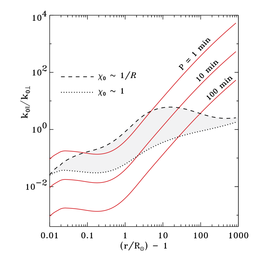
Figure 5.— Radial dependence of the modeled ratio of outer-scale wavenumbers $k_{0\parallel}/k_{0\perp}$ computed under various assumptions: constant inertial-frame frequencies (red solid curves, labeled by wave period), ideal Goldreich & Sridhar (1995) critical balance (dotted black curve), and modified Beresnyak & Lazarian (2008, 2009) critical balance (dashed black curve).

3.2. Solutions in the Absence of Coupling

Here we present some example results for the power spectra $E_{\rm A}(k_{\parallel},k_{\perp})$ and $E_{\rm F}(k_{\parallel},k_{\perp})$. These spectra are computed from Equations (31), (32), and (38) in the limiting cases of time independence and no mode coupling ($C_{\rm AF}=0$). The Alfvénic spectrum was first computed in its reduced form using the solutions for $b_{\perp}(k_{\perp})$ given in Appendices C.1 and C.2, and then it was expanded into full wavenumber space by using the results of Appendix C.3. The shape of the fast-mode spectrum was determined from the analytic solutions given in Appendices C.4 and C.5.

To illustrate the wavenumber dependence of the power spectra, we chose a single coronal height $z=10\,R_{\odot}$ at which $\beta\approx 0.04$. We typically plot the wavenumbers in terms of dimensionless quantities $k_{\parallel}V_{\rm A}/\Omega_{p}$ and $k_{\perp}\rho_{p}$. Dissipative wave-particle interactions tend to become important when these quantities reach order-unity values, and ideal MHD conditions apply when these quantities are small. Typically, the driving scale for Alfvénic turbulence occurs at $k_{0\perp}\rho_{p}\approx 10^{-6}$ to $10^{-4}$, with the larger values generally occurring at larger heliocentric distances.

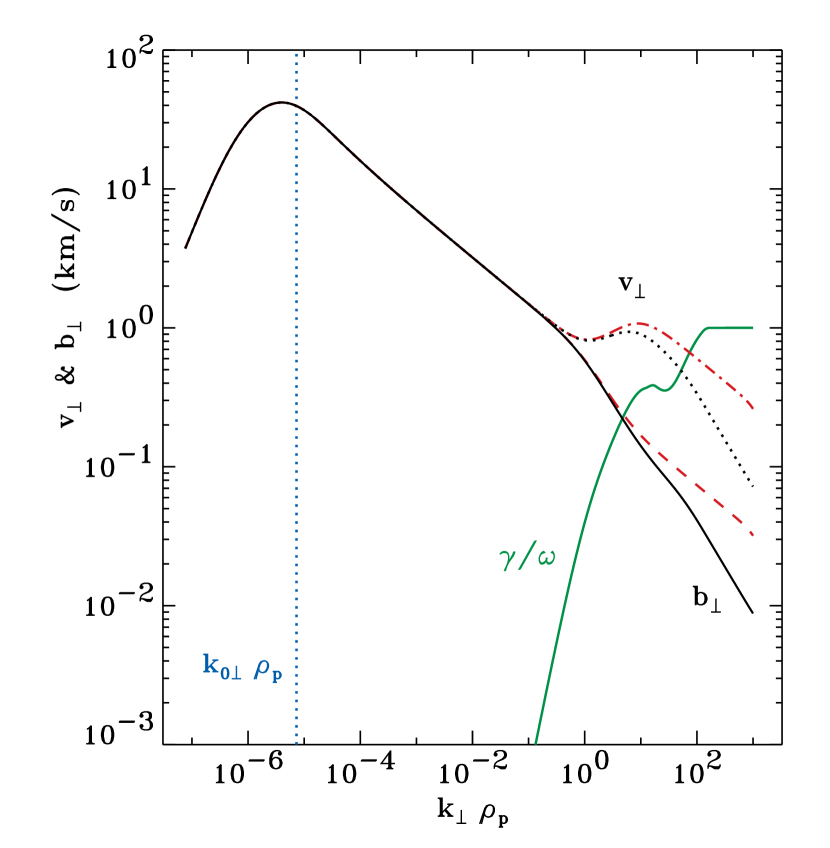
Figure 6.— Reduced Alfvénic fluctuation spectra for magnetic field and velocity fluctuations at $z=10\,R_{\odot}$, plotted as a function of $k_{\perp}\rho_{p}$. Undamped spectra for $b_{\perp}$ (red dashed curve) and $v_{\perp}$ (red dot-dashed curve) are compared with damped spectra for $b_{\perp}$ (black solid curve) and $v_{\perp}$ (black dotted curve). The dimensionless KAW dissipation rate $\tilde{\gamma}/\omega$ used to compute the damped spectra is also shown (green solid curve), as is the location of the perpendicular outer scale $k_{0\perp}\rho_{p}$ (blue dotted line).

In Figure 6 we show the time-steady $k_{\perp}$ dependence for the Alfvénic $b_{\perp}$ and $v_{\perp}$ fluctuations, both with and without KAW dissipation. To set the cascade properties, we utilized the values of the constants given in Section 3.1, and we also assumed $s=\mu_{\perp}/\alpha_{\perp}=2$ and $k_{0\parallel}/k_{0\perp}=0.1$. The KAW damping ratio $\tilde{\gamma}/\omega$ appropriate for the assumed value of $\beta$, which was used in Equation (C11), is also shown in green (see also Section 5). At the outer scale, the peak value of $v_{\perp}$ is 42 km s^-1. We caution that this value should not be assumed to be equivalent to the full rms velocity amplitude. In this case, $(U_{\rm A}/\rho_{0})^{1/2}=196$ km s^-1, which is almost a factor of 5 larger than the maximum value of $v_{\perp}$ at this height.

The damped spectra shown in Figure 6 have several features that resemble those of measured KAWs in the solar wind. Using the conventional form of the reduced energy spectrum ($e_{\rm A}\approx b_{\perp}^{2}/k_{\perp}$) we found that the magnetic fluctuation power made a transition from a Kolmogorov-like power law $k_{\perp}^{-5/3}$ to a steeper spectrum with $k_{\perp}^{-2.5}$ at $k_{\perp}\rho_{p}\approx 1$. The spectrum becomes shallower again around $k_{\perp}\rho_{p}\approx 40$ because the wavenumber dependence of $\phi$ flattens out at low values of $\beta$. This behavior is reminiscent of that predicted by Voitenko & De Keyser (2011). At larger radial distances where $\beta\gtrsim 1$, the KAW dispersion relation (Equation (35)) gives rise to a more sustained increase in $\phi$ with increasing $k_{\perp}$. This in turn produces spectra that remain steep, with $e_{\rm A}\propto k_{\perp}^{-2.5}$ persisting over several orders of magnitude of $k_{\perp}$ in agreement with both measurements (Smith et al., 2006; Sahraoui et al., 2010) and other models (Howes et al., 2008). We note that the predicted undamped KAW power-law decline of $k_{\perp}^{-7/3}$ (see Appendix C.1) was not seen for any sustained range of $k_{\perp}$.

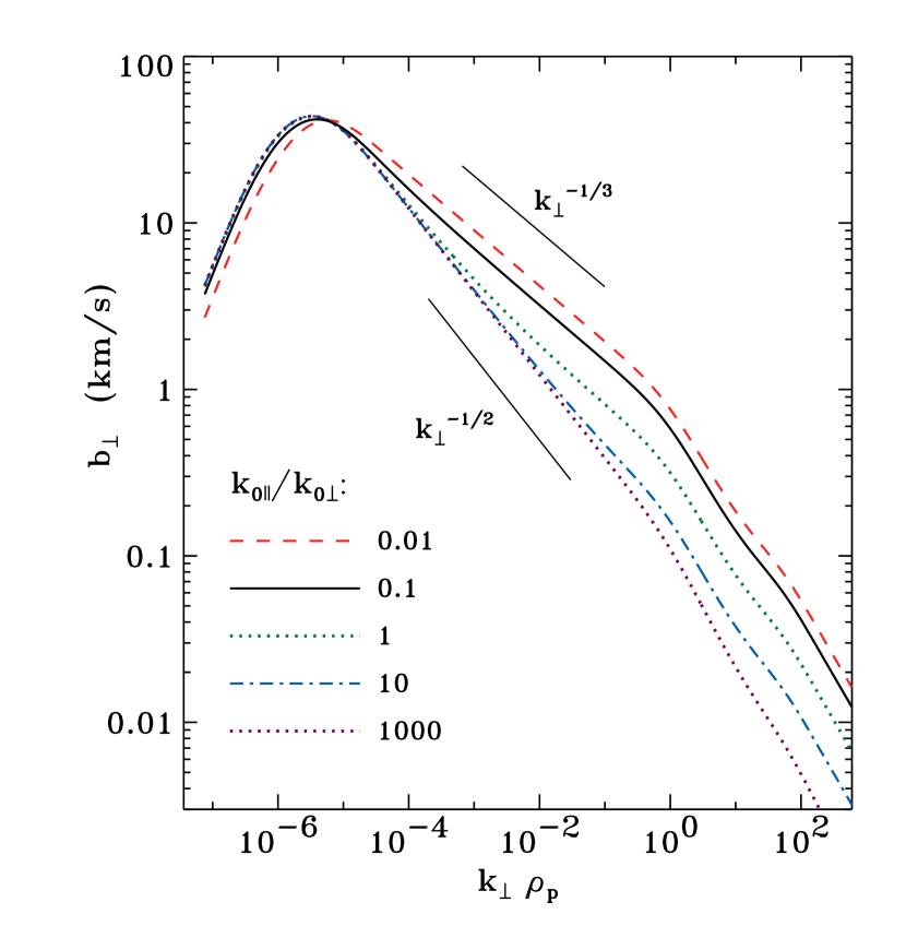
Figure 7.— Reduced Alfvénic magnetic spectra at $z=10\,R_{\odot}$, computed assuming different values of $k_{0\parallel}/k_{0\perp}=0.01$ (red dashed curve), 0.1 (black solid curve), 1 (green dotted curve), 10 (blue dot-dashed curve), and 1000 (violet dotted curve).

Figure 7 shows the result of varying the normalization of the parallel outer scale wavenumber $k_{0\parallel}$ on the shape of $b_{\perp}(k_{\perp})$. We kept the same value of $s=2$ that was used in Figure 6, but we varied the constant ratio $k_{0\parallel}/k_{0\perp}$ over five orders of magnitude. For the lowest values of $k_{0\parallel}$ the outer-scale critical balance ratio $\chi_{0}$ always remains much smaller than unity. This means that the stirring or forcing takes place well within the “filled” region of wavenumber space, and thus strong turbulence occurs. In this case, $b_{\perp}\propto k_{\perp}^{-1/3}$ and thus $e_{\rm A}\propto k_{\perp}^{-5/3}$. The opposite extreme case of large $k_{0\parallel}$ corresponds to $\chi_{0}\gg 1$ and weak turbulence with less anisotropic driving. In that limit, the inertial range spectra are given by $b_{\perp}\propto k_{\perp}^{-1/2}$ and $e_{\rm A}\propto k_{\perp}^{-2}$. Our model shows the gradual transition between these two extreme cases.

In Figure 8 we compare the Alfvén and fast-mode spectra with one another. As above, we used the background conditions at a coronal height of $z=10\,R_{\odot}$ and we assumed $k_{0\parallel}/k_{0\perp}=0.1$. We illustrate the most extreme case of a lack of high-frequency Alfvénic power by showing the contours of $E_{\rm A}(k_{\parallel},k_{\perp})$ for the case $s\rightarrow\infty$. In this limit, Equation (C16) describes an exponential decrease of power with increasing $\chi$. Other comparable examples of this kind of spectrum can be found in Figure 4b of Cranmer & van Ballegooijen (2003) and Figures 1 and 2 of Jiang et al. (2009). We computed the Alfvénic and fast-mode spectra with the kinetic sources of damping that were described in Section 5. Note that $E_{\rm F}$ experiences the strongest damping at intermediate values of $\theta$. For $\theta\lesssim 10^{\circ}$ or $\theta\gtrsim 85^{\circ}$, the transit-time damping described by Equation (58) is relatively weak.

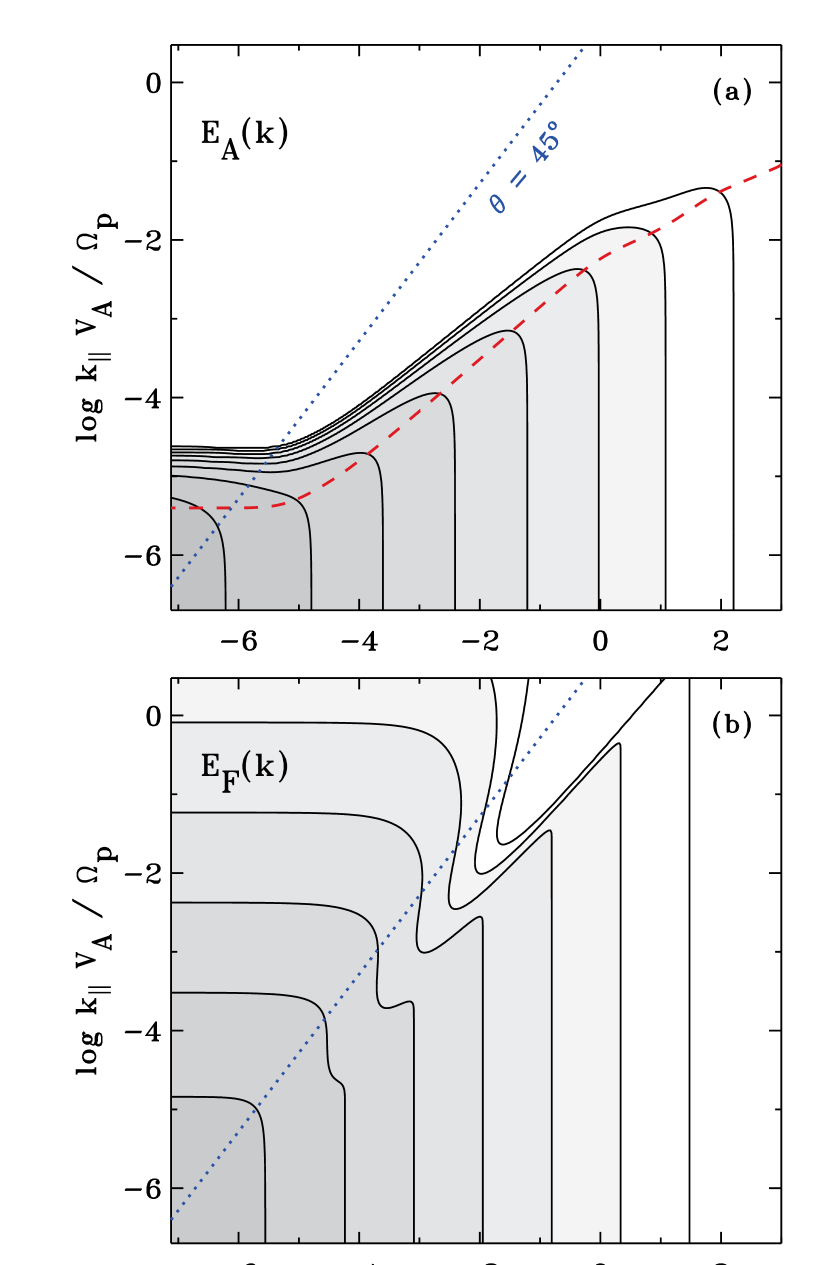
Figure 8.— Comparison of uncoupled power spectra at $z=10\,R_{\odot}$ for (a) Alfvénic fluctuations, $E_{\rm A}(k_{\parallel},k_{\perp})$, and (b) fast-mode fluctuations, $E_{\rm F}(k_{\parallel},k_{\perp})$. Contours are plotted one per $10^{4}$ (i.e., one every four decades in power) from $10^{-1}$ down to $10^{-29}$ times the maximum value of $E_{\rm A}$. Darker shading denotes higher power levels. Also shown is a line denoting $\theta=45^{\circ}$ (blue dotted curve) and the critical balance locus of points that obey $\chi_{\rm eff}=1$ (red dashed curve).

4. Coupling Between Alfvén and Fast-Mode Waves

4.1. Basic Physics and Phenomenological Rates

There are several ways that the ideal linear MHD wave modes can become coupled to one another in the corona and solar wind:

1. Inhomogeneities in the background plasma can blur the definitions of the individual modes. For example, linear reflection due to radial variations in $V_{\rm A}$ (Ferraro & Plumpton, 1958; Heinemann & Olbert, 1980) may produce not only incoming Alfvén waves (i.e., $0<{\cal R}<1$), but also fast and slow magnetosonic waves (e.g., Stein, 1971; McDougall & Hood, 2007). In addition, large-scale bends in the background magnetic field ${\bf B}$ (Frisch, 1964; Wentzel, 1974), density variations between flux tubes (Valley, 1974; Markovskii, 2001; Mecheri & Marsch, 2008), or velocity shears (Poedts et al., 1998; Gogoberidze et al., 2007) can drive instabilities that partially convert Alfvén waves into other modes.

2. Even in a homogeneous medium, the MHD waves begin to lose their ideal linear character when their amplitudes become large. Nonlinear Alfvén waves naturally drive second order fluctuations in $v_{\parallel}$ and $\delta\rho$ that mimic the properties of both slow and fast magnetosonic waves (Hollweg, 1971; Spangler, 1989; Vasquez & Hollweg, 1999). Large-amplitude waves also excite a range of wave-wave interactions that can often be characterized either as two modes giving birth to a third, or one mode splitting into several others (e.g., Chin & Wentzel, 1972; Goldstein, 1978; Del Zanna et al., 2001; Sharma & Kumar, 2010). Models of weak turbulence, in which the wave-wave interactions describe the cascade process (Chandran, 2005, 2008a; Luo & Melrose, 2006; Yoon & Fang, 2008) also create this kind of coupling.

3. Although not strictly a multi-mode coupling, when $k_{\perp}\rho_{p}\gtrsim 1$ the Alfvén mode begins to exhibit oscillations in density, parallel electron velocity, and the parallel electric and magnetic fields (Hasegawa & Chen, 1976; Hollweg, 1999). Observationally, it has proved difficult to separate such dispersive KAW density fluctuations from those arising from independent sources of fast or slow MHD waves (e.g., Harmon & Coles, 2005; Chandran et al., 2009).

In this paper we take account of one particular nonlinear effect from the second entry in the above list. Specifically, Chandran (2005) suggested that weak turbulence couplings between Alfvén and fast-mode fluctuations may provide enough power at high $k_{\parallel}$ to induce substantial ion cyclotron heating. Suzuki et al. (2007) argued that this effect may be relatively unimportant because the fast-mode cascade timescale $\tau_{\rm F}$ is long in comparison to the Alfvén cascade timescale $\tau_{\rm A}$. This may be the case in the low-frequency regime of wavenumber space where $\chi\ll 1$, but at the cyclotron resonant frequencies of interest ($k_{\parallel}\sim\Omega_{p}/V_{\rm A}$) the Alfvénic cascade is quenched because $\chi\gg 1$. The fast-mode cascade may in fact even be faster than any intrinsic Alfvénic spectral transfer in this region of wavenumber space. Therefore, we proceed using the Chandran (2005) results for Alfvén/fast-mode coupling.

We express the coupling term in Equations (31)–(32) as

$$C_{\rm AF}\,=\,\frac{E_{\rm F}-E_{\rm A}}{\tau_{\rm AF}}$$ (46)

such that, in the absence of other processes, the power spectra at a given wavenumber ${\bf k}$ are driven toward a common value over a coupling timescale $\tau_{\rm AF}({\bf k})$. The weak turbulence model of Chandran (2005) gave an approximate value for this timescale of

$$\tau_{\rm AF}\,\approx\,\frac{15}{23\pi^{2}}\tau_{\rm F}\,\sin^{2}\theta$$ (47)

which holds in the limiting cases of $E_{\rm F}>E_{\rm A}$ and nearly parallel propagation ($\theta\ll 1$). In the opposite case of $E_{\rm A}\gg E_{\rm F}$, it’s likely that $\tau_{\rm AF}$ would no longer depend linearly on $\tau_{\rm F}$, and may scale instead with $\tau_{\rm A}$. However, the region of wavenumber space with which we are most concerned is the high-$k_{\parallel}$, low-$\theta$ ion cyclotron regime. At those wavenumbers, we know that in the absence of coupling the condition $E_{\rm F}\gg E_{\rm A}$ is likely to be satisfied, and the coupling will be a transfer of energy from the dominant fast-mode spectrum to the much less intense Alfvén mode.

The wave-wave conditions of frequency and wavenumber matching (e.g., Sagdeev & Galeev, 1969) confirm that the most rapid coupling should occur when the dispersive properties of the Alfvén and fast-mode waves are the most similar to one another; i.e., at $\theta\rightarrow 0$. Note that Equation (39) gave $\tau_{\rm F}\propto 1/\sin\theta$, so the combined dependence for the coupling time is $\tau_{\rm AF}\propto\sin\theta$. In practice, however, we found that using this ideal expression for $\tau_{\rm AF}$ could lead to an unphysical singularity at $\theta=0$. We removed this singularity by replacing $\theta$ in Equation (47) by $\theta+\delta\theta$. We set $\delta\theta$ to a constant value of 0.01 to avoid having an infinitely fast coupling rate at parallel propagation. To retain the most generality, we chose to reparameterize the coupling timescale as

$$\tau_{\rm AF}\,=\,\frac{1}{\Phi}\,\tau_{\rm F}\sin^{2}(\theta+\delta\theta)$$ (48)

where we find it useful to vary the constant coupling strength $\Phi$ up or down from the value of $23\pi^{2}/15\approx 15.1$ derived by Chandran (2005). The case $\Phi=0$ corresponds to ignoring the coupling altogether.

Note that the above form for the coupling timescale implies that $\tau_{\rm AF}\propto k_{\perp}/k^{3/2}$, so that the coupling is rapid at wavenumbers corresponding to ion cyclotron resonance (large $k_{\parallel}$, small $k_{\perp}$). The coupling is much slower at KAW wavenumbers favored by the pure Alfvénic cascade (small $k_{\parallel}$, large $k_{\perp}$). Thus, the bulk of the Alfvénic spectrum at $\chi\ll 1$ is likely to be more or less unaffected by the coupling. This seems to be consistent with our assumption that the integrated energy densities $U_{\rm A}$ and $U_{\rm F}$ also remain uncoupled from one another. We realize that this may be a severe underestimate of the degree of energy transfer between Alfvén and magnetosonic modes in the corona and solar wind. However, one main purpose of this paper is to investigate how much can be accomplished with only this small degree of coupling in the high-$k_{\parallel}$ tails of the power spectra.

4.2. Approximate Solutions for Coupled Spectra

The exact solutions to Equations (31) and (32) with coupling ($C_{\rm AF}\neq 0$) must be found numerically. Here we present an approximate solution that is both (1) likely to reflect the proper behavior of more rigorous numerical solutions in many limiting regimes of parameter space, and (2) efficient to implement on a large grid of model spectra spanning a wide range of heliocentric distances. We begin by approaching the problem iteratively; i.e., we solve Equation (31) for $E_{\rm A}$ under the assumption that $E_{\rm F}$ is known, and we then solve Equation (32) for $E_{\rm F}$ under the assumption that $E_{\rm A}$ is known. The analytic solutions derived below suggest a natural way to terminate this iteration after only one round.

When solving the advection-diffusion equation for Alfvénic fluctuations, let us temporarily ignore the outer-scale source term $S_{\rm A}$ and the dissipation-range damping term that depends on $\gamma_{\rm A}$. Since we are most concerned with the generation and transport of wave power in the high-$k_{\parallel}$ regions that undergo ion cyclotron resonance, we consider the weak turbulence regime of $\chi\gg 1$, in which the transport of energy is mainly from low to high $k_{\perp}$ and there is negligible parallel spreading (see also Oughton et al., 2006). Thus, we solve the advection-diffusion equation for discrete, non-interacting “strips” of wavenumber space each having constant $k_{\parallel}$. The nonlinear coupling supplies wave energy locally, and the Alfvénic cascade takes it from low to high $k_{\perp}$. If we simplify further by assuming pure advection (i.e., $\alpha_{\perp}=0$), the time-steady version of Equation (31) becomes

$$\frac{\mu_{\perp}}{k_{\perp}}\frac{\partial}{\partial k_{\perp}}\left(\frac{k_{\perp}^{2}E_{\rm A}}{\tau_{\rm A}}\right)\,=\,\frac{E_{\rm F}-E_{\rm A}}{\tau_{\rm AF}}\,\,,$$ (49)

where we use Equation (A6) to give the timescale $\tau_{\rm A}\approx\chi/(k_{\perp}v_{\perp})$ in the weak turbulence regime, and we use Equation (48) for $\tau_{\rm AF}$.

The above advection-coupling equation can be rewritten as a first-order ordinary differential equation,

$$\frac{\partial E_{\rm A}}{\partial k_{\perp}}+\left(\frac{10}{3k_{\perp}}+\frac{f_{0}}{k_{\perp}^{10/3}}\right)E_{\rm A}\,=\,\frac{f_{0}E_{\rm F}}{k_{\perp}^{10/3}}$$ (50)

where

$$f_{0}\,=\,\frac{\Phi}{\mu_{\perp}}\left(\frac{v_{0{\rm F}}}{v_{0\perp}}\right)^{2}\frac{k_{0{\rm F}}^{1/2}k_{\parallel}^{5/2}}{k_{0\perp}^{2/3}}\,\,.$$ (51)

To obtain Equation (50), we made several power-law assumptions for the timescales $\tau_{\rm A}$ and $\tau_{\rm AF}$, which depend on the velocity spectra $v_{\perp}$ (for Alfvén waves) and $v_{k}$ (for fast-mode waves), respectively, with

$$v_{\perp}\,=\,v_{0\perp}\left(\frac{k_{\perp}}{k_{0\perp}}\right)^{-1/3}\,\,,\,\,\,\,v_{k}\,=\,v_{0{\rm F}}\left(\frac{k}{k_{0{\rm F}}}\right)^{-1/4}\,\,.$$ (52)

We also assumed that we are solving for $E_{\rm A}$ mainly in the small-$\theta$ region of wavenumber space in which $k\approx k_{\parallel}$.

With the above assumptions taken into account, Equation (50) can be solved by means of an integrating factor. We first define the dimensionless independent variable

$$y\,=\,\frac{3f_{0}}{7k_{\perp}^{7/3}}\,=\,\left(\frac{k_{c}}{k_{\perp}}\right)^{7/3}$$ (53)

which is a measure of the relative strength of the nonlinear coupling. When $y\gg 1$ (or $k_{\perp}\ll k_{c}$) the coupling is strong and we should expect $E_{\rm A}\approx E_{\rm F}$. When $y\ll 1$ (or $k_{\perp}\gg k_{c}$) the coupling is weak in comparison to the cascade and we expect $E_{\rm A}\ll E_{\rm F}$. Note also that $y$ depends much more sensitively on $\theta$ than on the magnitude $k$. Working through the integrating factor method and choosing an integration constant of zero (to avoid the solution diverging to infinity when $y\gg 1$), we obtain

$$E_{\rm A}\,=\,\frac{7y}{3}\left[1-e^{y}y^{3/7}\,\Gamma\left(\frac{4}{7},\,y\right)\right]E_{\rm F}$$ (54)

where $\Gamma(a,y)$ is the incomplete gamma function. This function behaves as expected in the limits of strong and weak coupling as discussed above.

Next we solve the coupled fast-mode advection-diffusion equation for $E_{\rm F}$ under the assumption that $E_{\rm A}$ is known. Making use of many of the same simplifications that were used to solve the $E_{\rm A}$ equation, we include only the cascade and coupling terms, with

$$\frac{\alpha_{\rm F}}{k^{2}}\frac{\partial}{\partial k}\left(k^{2}D_{\rm F}\frac{\partial E_{\rm F}}{\partial k}\right)\,=\,C_{\rm AF}\,=\,\left[\frac{1}{\tau_{\rm AF}}\left(1-\frac{E_{\rm A}}{E_{\rm F}}\right)\right]E_{\rm F}\,\,.$$ (55)

Noticing that the quantity in square brackets above is an effective damping rate $\gamma_{\rm eff}$, we use Equation (54) to write the ratio $E_{\rm A}/E_{\rm F}$ as a known function of $k_{\parallel}$ and $k_{\perp}$. After substituting in the wavenumber dependence for $\tau_{\rm AF}$, we found that $\gamma_{\rm eff}\propto(k/k_{0{\rm F}})^{1/2}$. The analytic solution of $E_{\rm F}(k)$ for this special case is given in Equation (C32), and the constant $c_{\gamma}$ in that expression is specified here to be

$$c_{\gamma}\,=\,\frac{8\Phi}{49\,\alpha_{\rm F}\sin^{2}\theta}\left(1-\frac{E_{\rm A}}{E_{\rm F}}\right)\,\,.$$ (56)

The solution of Equation (C32) is applied only for $k\geq k_{0{\rm F}}$, and the uncoupled/undamped fast-mode power spectrum $E_{0{\rm F}}$ is used for $k<k_{0{\rm F}}$.

Since our solution for the ratio $E_{\rm A}/E_{\rm F}$ depends only on wavenumber and not on any prior solutions of $E_{\rm A}$ or $E_{\rm F}$, we found that there is no need for further iteration. We solve first for $E_{\rm F}$ as described above, using Equation (54) for the ratio $E_{\rm A}/E_{\rm F}$, and then we use this ratio to solve for $E_{\rm A}$. Note that the complete solution for $E_{\rm F}$ must take account of both coupling and transit-time damping (i.e., the damping rate given by Equation (58)). In practice, we apply both types of damping separately to the uncoupled and undamped fast-mode power spectrum $E_{0{\rm F}}$ and we use the solution that gives rise to stronger local damping at any given wavenumber. At high enough values of $k_{\parallel}$, the complete solution for $E_{\rm A}$ must take into account the effects of ion cyclotron damping. We use the approximate prescription given by Equation (C20) to implement this damping.

If the original uncoupled spectra obey $E_{0{\rm A}}\leq E_{0{\rm F}}$, then the coupled spectra follow

$$E_{0{\rm A}}\leq E_{\rm A}\leq E_{\rm F}\leq E_{0{\rm F}}$$

at wavenumbers in the high-$k_{\parallel}$ regime where the coupling is applied. Usually, the relative increase in $E_{\rm A}$ from its uncoupled solution is greater than the relative decrease in $E_{\rm F}$ from its uncoupled solution. In all cases, however, we found that the variations in the spectra introduced by the coupling do not significantly affect the total wavenumber-integrated power in either $E_{\rm A}$ or $E_{\rm F}$.

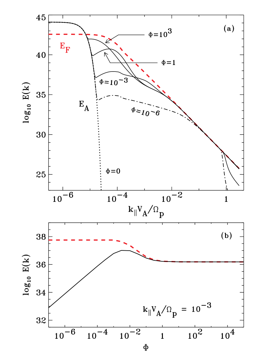
Figure 9.— (a) Slices of time-steady spectra at $z=10\,R_{\odot}$, shown at constant $k_{\perp}=k_{0\perp}$: uncoupled spectra $E_{0{\rm A}}$ (black dotted curve) and $E_{0{\rm F}}$ (red dashed curve), and coupled $E_{\rm A}$ spectra that were computed with a range of $\Phi$ values (black solid curves). (b) Variation of $E_{\rm A}$ (black solid curve) and $E_{\rm F}$ (red dashed curve) with $\Phi$, shown at constant wavenumber $k_{\perp}=k_{0\perp}$ and $k_{\parallel}V_{\rm A}/\Omega_{p}=10^{-3}$.

Figure 9 illustrates the effects of including coupling on $E_{\rm A}$. As in earlier plots of spectrum results, we used the representative height $z=10\,R_{\odot}$ and we assumed $k_{0\parallel}=k_{0\perp}/10$. In order to show that the coupling can be efficient even when the uncoupled Alfvén wave power $E_{0{\rm A}}$ is negligibly small, we assumed the extreme limiting case of $s\rightarrow\infty$. In Figure 9(a) we show the $k_{\parallel}$ dependence of the spectra along a slice taken at a constant value of $k_{\perp}=k_{0\perp}$. We varied the parameter $\Phi$ between $10^{-6}$ and $10^{+3}$. Even if the coupling is several orders of magnitude weaker than estimated by Chandran (2005), it is still likely to be efficient at generating some Alfvénic wave power at $k_{\parallel}\approx\Omega_{p}/V_{\rm A}$. However, if the coupling constant $\Phi$ is significantly smaller than $\sim$10^-3, the ion cyclotron damping at $k_{\parallel}\approx\Omega_{p}/V_{\rm A}$ is likely to overwhelm the “local supply” of wave energy from the coupling and give rise to a low level of resonant wave power.

Figure 9(b) shows how the power at a given wavenumber ($k_{\perp}=k_{0\perp}$ and $k_{\parallel}V_{\rm A}/\Omega_{p}=10^{-3}$) varies as a function of $\Phi$. The fast-mode power decreases monotonically as $\Phi$ is increased, which confirms our treatment of the coupling in Equation (55) as an effective damping. The Alfvénic power generally increases (from its uncoupled value far below the lower edge of the plot) with increasing $\Phi$, but there is some nonmonotonicity around $\Phi\approx 10^{-2}$. This gives rise to a slightly counter-intuitive result that there may be more $E_{\rm A}$ power at high-$k_{\parallel}$ (and thus more proton and ion heating) at some values of $\Phi$ than in the $\Phi\rightarrow\infty$ limit.

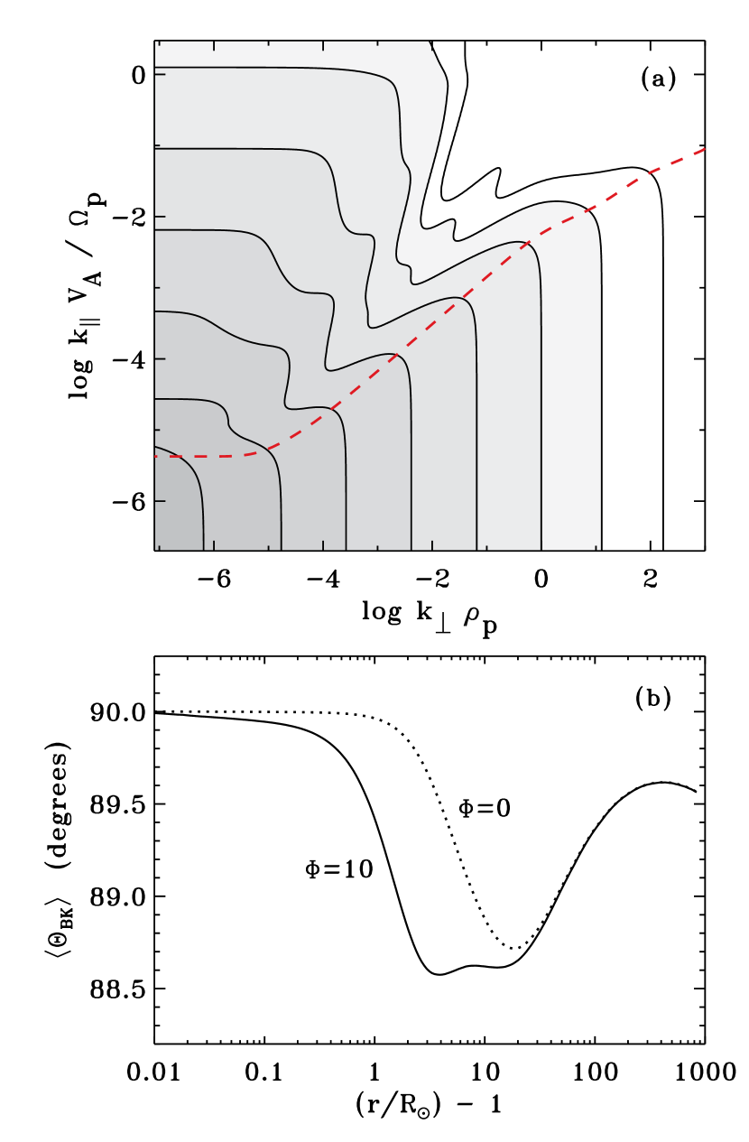
Figure 10.— (a) Contours of the $E_{\rm A}$ power spectrum, as in Figure 8 but computed with full fast-mode coupling ($\Phi=10$). (b) Radial dependence of spectrum-averaged angle $\Theta_{{\rm B}k}$ between the background field direction and the wavenumber vector ${\bf k}$, computed for $\Phi=10$ (solid curve) and for $\Phi=0$ (dotted curve).

An example of the full wavenumber dependence of the coupled $E_{\rm A}(k_{\parallel},k_{\perp})$ spectrum is shown in Figure 10(a) for a radial distance of $r=10\,R_{\odot}$. This model has the same parameters as the one shown in Figure 8, except that we set $\Phi=10$. Despite the appearance of substantial wave power at large values of $k_{\parallel}$, most of the power is still contained within the critical balance locus of $\chi\lesssim 1$. This is illustrated in another way by Figure 10(b), in which we show the radial dependence of the spectrum-averaged angle $\Theta_{{\rm B}k}$ between the background field direction and the wavenumber vector ${\bf k}$. We used a definition for the spectrum-averaged wavevector anisotropy that is similar to that of Gary et al. (2010),

$$\tan^{2}\langle\Theta_{{\rm B}k}\rangle\,=\,\frac{\int d^{3}{\bf k}\,\,E_{\rm A}({\bf k})\,k_{\perp}^{2}}{\int d^{3}{\bf k}\,\,E_{\rm A}({\bf k})\,k_{\parallel}^{2}}\,\,.$$ (57)

Note that the model result at $r=1$ AU (89.5°) is reasonably close to the value of $\sim$88° measured by Sahraoui et al. (2010) from the four Cluster satellites at 1 AU. It is evident that a strongly perpendicular (“quasi-two-dimensional”) sense of wavenumber anisotropy is not incompatible with the existence of high-frequency ion cyclotron resonant wave power.

5. Kinetic Dispersion and Dissipation

When computing the dissipation rates $\gamma_{\rm A}$ and $\gamma_{\rm F}$, we are careful to distinguish between two conceptually different sources of damping. First, there are the collisional and outer-scale cascade processes that were included in Equation (17). These processes act at low wavenumber and drive the overall radial evolution of the wave energy densities $U_{\rm A}$ and $U_{\rm F}$. We do not include them in the damping terms in Equations (31)–(32) because their net effects are already included in the source terms $S_{\rm A}$ and $S_{\rm F}$. Second, there are the largely collisionless kinetic processes that become dominant at large wavenumbers. These are the actual processes that dissipate the power and give rise to heating, and we describe them in the remainder of this section.

Once the power levels of Alfvénic and fast-mode fluctuations are specified as detailed functions of $k_{\parallel}$, $k_{\perp}$, and radial distance, we compute their damping rates and species-dependent heating rates from linear Vlasov theory. Although it is known that strong MHD turbulence is far from “wavelike” (i.e., coherent wave packets do not survive for more than about one period before being shredded by the cascade), there is a long history of using damped linear wave theory to study the small-scale dissipation of such a cascade (see, e.g., Eichler, 1979; Quataert, 1998; Leamon et al., 1999; Quataert & Gruzinov, 1999; Marsch & Tu, 2001a; Cranmer & van Ballegooijen, 2003; Gary & Borovsky, 2004; Harmon & Coles, 2005). A typical justification of this approach is that no matter the strength of the fluctuations at the outer scale, once the cascade reaches the high-$k$ dissipation range the magnitudes are much smaller and quite linear; see also Spangler (1991) and Lehe et al. (2009).

For the Alfvén waves, we utilize the Vlasov-Maxwell code described by Cranmer & van Ballegooijen (2003) and Cranmer et al. (2009) to solve the “warm” linear dispersion relation for the real and imaginary parts of the frequency in the solar wind frame ($\omega=\omega_{r}+i\gamma$) assuming a known real wavevector ${\bf k}$. The code uses the Newton-Raphson technique to isolate individual solutions from a grid of starting guesses in $\omega_{r}$, $\gamma$ space, and we select only the left-hand-polarized (Alfvénic) solutions. We assumed homogeneous plasma conditions and isotropic Maxwellian velocity distributions (with $T_{p}=T_{e}$), and we ran the code for a range of assumed values of $\beta$ between $10^{-3}$ and $10^{2}$. The code also provides the partition fractions of wave energy in electric, magnetic, kinetic, and thermal perturbations for each wave mode (see also Krauss-Varban et al., 1994).

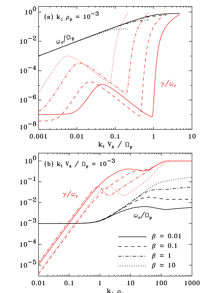
Figure 11.— Linear dispersion properties of Alfvén waves computed for a range of plasma $\beta$ values. (a) Real frequencies $\omega_{r}/\Omega_{p}$ (black curves) and damping rates $\gamma/\omega_{r}$ (red curves) plotted versus $k_{\parallel}$ at constant $k_{\perp}\rho_{p}=10^{-3}$, for $\beta=0.01$ (solid curves), $\beta=0.1$ (dashed curves), $\beta=1$ (dot-dashed curves), $\beta=10$ (dotted curves). (b) Same quantities as in panel (a), but shown as a function of $k_{\perp}$ at constant $k_{\parallel}V_{\rm A}/\Omega_{p}=10^{-3}$.

Figure 11 shows several example solutions for the real and imaginary parts of the frequency along one-dimensional cuts through wavenumber space. For simplicity, we present all damping rates $\gamma$ as their absolute values, since strictly speaking the solutions from the Vlasov-Maxwell code all have $\gamma<0$. Figure 11(a) illustrates the approach to the ion cyclotron resonance regime by holding $k_{\perp}$ constant at a small value and plotting $\omega_{r}$ and $\gamma$ versus $k_{\parallel}$. Note the cessation of weakly damped solutions at $\gamma\approx\omega_{r}\approx\Omega_{p}$, which takes place at lower values of $k_{\parallel{\rm max}}$ for higher values of $\beta$. Equation (C18) is a parameterized fit to the $\beta$-dependence of this cutoff wavenumber.

Figure 11(b) shows the approach to the high-$k_{\perp}$ KAW dissipation limit for a constant small value of $k_{\parallel}$. When solving the dispersion relation along a succession of increasing values of $k_{\perp}$, there are sometimes small discontinuities in slope between neighboring solutions (especially in strongly damped regions where $|\gamma/\omega_{r}|\gtrsim 0.5$). Nonetheless, the dispersion properties of our solutions remain sufficiently “KAW-like” to represent a continuous set of damping rates from low to high $k_{\perp}$. The behavior of $\omega_{r}$ versus $k_{\perp}$ agrees reasonably well with the approximate expression given by Equation (35). For values of $\beta\gtrsim 1$, there are secondary maxima in $\gamma/\omega_{r}$ at $k_{\perp}\rho_{p}\approx 1$ that come from proton Landau damping, whereas the larger rates at $k_{\perp}\rho_{p}>10$ are dominated by electron Landau damping. The damping rates shown in Figure 11(b) were also used as the effective KAW ratios $\tilde{\gamma}_{\rm A}/\omega_{r}$ described in Appendix C.2. These rates were used to compute the high-$k_{\perp}$ dissipation of $b_{\perp}$ and $v_{\perp}$ as shown in Figures 6 and 7.

For the fast-mode waves, we make use of a parameterized expression for the rate of transit-time damping, which in several studies was found to be the dominant kinetic process to dissipate this wave mode (e.g., Barnes, 1966; Perkins, 1973; Yan & Lazarian, 2004). Thus, we assume

$$\frac{\gamma_{\rm F}}{\omega_{r}}\,=\,\frac{\theta^{2}\sqrt{\pi\beta}}{4}\left(1+\frac{\theta^{2}}{\sqrt{\theta^{4}+4\Omega_{p}^{2}/\omega_{r}^{2}}}\right)$$

$$\times\,\,\sqrt{\frac{m_{e}}{m_{p}}}\exp\left(-\frac{m_{e}}{m_{p}\beta\cos^{2}\theta}\right)\,\,,$$ (58)

where $\omega_{r}$ is given by the ideal fast-mode dispersion relation of Equation (4). This expression was given by Yan & Lazarian (2004) based on initial calculations of Stepanov (1958). Equation (58) is valid strictly for only $\theta\ll 1$, but it does not diverge from the more exact solution at larger $\theta$ by more than about a factor of two.

The remainder of this section describes how the dissipated Alfvén wave energy is partitioned between protons, electrons, and heavy ions. We ignore the particle heating that comes from fast-mode wave dissipation because its overall magnitude was found to be small in comparison to that from Alfvén waves. In a pure hydrogen plasma, we separate the damping rate $\gamma$ into components attributed to the kinetic effects of protons and electrons. To zeroth order, the contribution to $\gamma$ from other ions is negligibly small and can be estimated separately (see below). Thus, we define $\gamma=\gamma_{p}+\gamma_{e}$, where

$$\gamma_{s}\,=\,\gamma\,\frac{\psi_{s}}{\psi_{p}+\psi_{e}}\,\,,$$ (59)

where $s=p,e$ denotes either the protons or electrons, and the species-dependent resonance functions are given by

$$\psi_{s}\,=\,\frac{\omega_{r}\omega_{ps}^{2}}{k_{\parallel}w_{\parallel s}}\sum_{\ell=-\infty}^{+\infty}\exp\left(-\xi_{\parallel}^{2}-\xi_{\perp}^{2}\right)\sum_{m=\ell-1}^{\ell+1}a_{m}I_{m}(\xi_{\perp}^{2})\,\,,$$ (60)

where $\omega_{ps}^{2}=4\pi e^{2}n_{s}/m_{s}$ is the squared plasma frequency, $w_{\parallel s}$ and $w_{\perp s}$ are parallel and perpendicular thermal speeds of species $s$, and $I_{m}$ is the $m$-order modified Bessel function of the first kind. The dimensionless coefficients $a_{m}$ depend on the electric-field polarization vector that is output from the Vlasov-Maxwell dispersion code of Cranmer & van Ballegooijen (2003), and they are given in full by Equations (43)–(45) of Marsch & Tu (2001a). Equation (60) is valid for an isotropic Maxwellian distribution, for which $w_{\parallel s}=w_{\perp s}$ and there is assumed to be zero differential bulk flow between the protons and electrons. The dominance of ion cyclotron or Landau damping depends on the values of the dimensionless resonance factors,

$$\xi_{\parallel}=\frac{\omega-\ell\Omega_{s}}{k_{\parallel}w_{\parallel s}}\,\,,\,\,\,\,\xi_{\perp}=\frac{k_{\perp}w_{\perp s}}{\Omega_{s}\sqrt{2}}\,\,.$$ (61)

In practice, we truncate the infinite sum in Equation (60) at $-10\leq\ell\leq+10$. Test runs made with a larger range of summation indices produced no substantial differences from those using the default range.

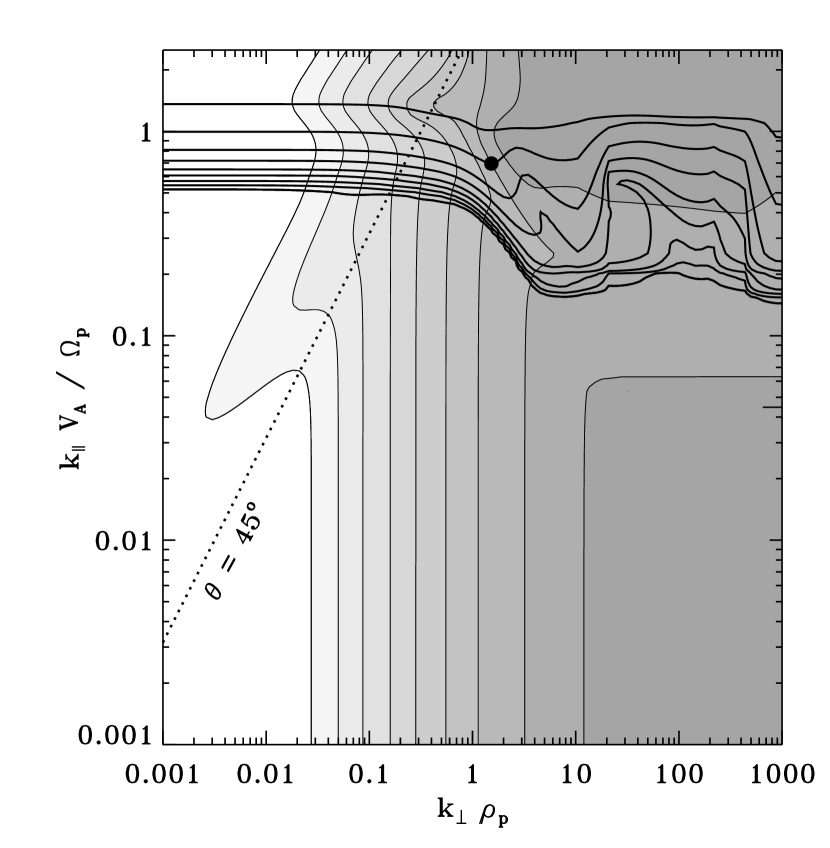
Figure 12.— Contours of $\gamma_{p}/\omega_{r}$ (thick curves) and $\gamma_{e}/\omega_{r}$ (thin curves separated by varying gray shading) plotted versus $k_{\parallel}$ and $k_{\perp}$. Contours are plotted twice per decade from $3\times 10^{-5}$ to $3\times 10^{-1}$ and generally go from low to high values with increasing wavenumber. A line denoting $\theta=45^{\circ}$ (dotted curve) and a point illustrating where $\theta_{ep}$ is defined (filled circle) are also shown.

Figure 12 shows separate sets of contours for $\gamma_{p}/\omega_{r}$ and $\gamma_{e}/\omega_{r}$ in wavenumber space for an example value of $\beta=0.1$. These contours can be compared with Figure 4(a) of Cranmer & van Ballegooijen (2003), which was computed for $\beta\approx 0.01$. The proton damping rate $\gamma_{p}/\omega_{r}$ increases rapidly as $k_{\parallel}V_{\rm A}/\Omega_{p}$ approaches unity, and the electron damping rate $\gamma_{e}/\omega_{r}$ increases more slowly as $k_{\perp}\rho_{p}$ increases from 0.1 to 100. The complex behavior of the contours in region of wavenumber space with both high $k_{\parallel}$ and high $k_{\perp}$ is the result of the dispersion relation being affected by the presence of strongly damped ion Bernstein modes (see, e.g., Stix, 1992; Howes et al., 2008).

It is evident from Figure 12 that, in the solar corona, the region of nearly parallel Alfvén wave propagation in wavenumber space (i.e., $\theta\ll 1$) is dominated by proton damping and the region of nearly perpendicular propagation ($\theta\rightarrow\pi/2$) is dominated by electron damping. The observational evidence for preferential proton and ion heating (Kohl et al., 2006) thus presents a problem when confronted with the dominant perpendicular anisotropy of Alfvénic turbulence.

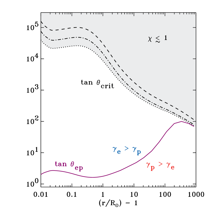
Figure 13.— Radial dependence of the tangents of $\theta_{ep}$ (solid purple curve) and $\theta_{\rm crit}$ (black curves), the latter computed for $k_{0\parallel}/k_{0\perp}=0.01$ (dotted), $k_{0\parallel}/k_{0\perp}=0.1$ (dot-dashed), and $k_{0\parallel}/k_{0\perp}=1$ (dashed). The gray region denotes the approximate region of parameter space expected to be “occupied” by a purely Alfvénic turbulent cascade.

Figure 13 illustrates the magnitude of this apparent discrepancy by comparing the large-scale radial dependence of two key angles. The strongly anisotropic Alfvénic cascade is illustrated by $\theta_{\rm crit}$, which is the angle between ${\bf k}$ and ${\bf B}_{0}$ at which occurs both the Goldreich & Sridhar (1995) critical balance ($\chi=1$) and the onset of KAW dispersion ($k_{\perp}\rho_{p}=1$). We find that $\tan\theta_{\rm crit}\approx V_{\rm A}/b_{\perp}$, where $b_{\perp}$ is evaluated at $k_{\perp}\rho_{p}=1$, and we plot $\tan\theta_{\rm crit}$ for three example values of the outer-scale wavenumber ratio $k_{0\parallel}/k_{0\perp}$. Figure 13 also shows the radial dependence of $\theta_{ep}$, which is defined as the angle at which the contours for $\gamma_{p}/\omega=0.1$ intersect with those of $\gamma_{e}/\omega=0.1$ in wavenumber space. (This point is shown in Figure 12 with a filled circle.) For $\theta<\theta_{ep}$ the damping is dominated by protons and ions; for $\theta>\theta_{ep}$ the damping is dominated by electrons. Note that $\theta_{ep}\ll\theta_{\rm crit}$ in the solar corona and much of the inner heliosphere, so that it is difficult to see how the cascade of linear Alfvén waves alone can be responsible for the observed proton and ion heating.

We computed the rates of proton and electron plasma heating from the modeled values of $\gamma_{p}$ and $\gamma_{e}$ by using the quasilinear framework outlined by Marsch & Tu (2001a) and Cranmer & van Ballegooijen (2003). The volumetric heating rates $Q_{s}$ (e.g., expressed in units of erg s^-1 cm^-3) are given by integrals over vector wavenumber $\bf k$ of the form

$$\frac{Q_{s}}{\rho}\,=\,\int d^{3}{\bf{k}}\,\,E_{\rm A}({\bf{k}})\,\,2\gamma_{s}$$ (62)

where $s=p,e$ denotes the particle type of interest. For now, we ignore differences between parallel and perpendicular heating and only compute the summed heating rate $Q_{s}=Q_{s\parallel}+Q_{s\perp}$. In order to perform the wavenumber integration in Equation (62), we constructed two-dimensional numerical grids of $\gamma_{p}$ and $\gamma_{e}$ for values of $10^{-3}\Omega_{p}/V_{\rm A}\leq k_{\parallel}\leq k_{\parallel{\rm max}}$ and $10^{-3}\leq k_{\perp}\rho_{p}\leq 10^{3}$. We used 200 points in $k_{\parallel}$ and 100 points in $k_{\perp}$, and we constructed a total of 14 grids for values of $\beta$ ranging from $10^{-3}$ to 22 (with $\beta$ varying logarithmically with three samples per decade). Linear interpolation was used to evaluate the damping rates at values of $k_{\parallel}$, $k_{\perp}$, and $\beta$ between the discrete grid points. We assumed that the ratios $\gamma_{p}/\omega_{r}$ and $\gamma_{e}/\omega_{r}$ remain constant as one extrapolates into the weakly-damped regions defined by $k_{\perp}\rho_{p}<10^{-3}$ and $k_{\parallel}V_{\rm A}/\Omega_{p}<10^{-3}$.

To estimate the heating rates experienced by heavy ions, we assume that most low-abundance ions do not have a significant effect on the overall wave dispersion relation. This allows us to use an “optically thin” resonance condition for the ion cyclotron wave-particle interaction (Cranmer, 2000), which results in a perpendicular heating rate

$$\frac{Q_{\perp i}}{m_{i}n_{i}}\,\approx\,\frac{\pi\Omega_{i}^{2}}{V_{\rm A}}\left(1-\frac{Z_{i}}{A_{i}}\right)\int d^{3}{\bf{k}}\,\,E_{\rm A}({\bf{k}})\,\,\delta(k_{\parallel}-\Omega_{i}/V_{\rm A})\,\,,$$ (63)

where $Z_{i}$ and $A_{i}$ are the ion charge and mass in proton units (see also Cranmer, 2001; Tu & Marsch, 2001; Landi & Cranmer, 2009). The Dirac delta function extracts a one-dimensional “strip” of the power spectrum that is in resonance with the ion Larmor motions at $\omega_{r}\approx k_{\parallel}V_{\rm A}=\Omega_{i}$. Thus, Equation (63) can be evaluated with just a single integration along the $k_{\perp}$ direction.

6. Results for Collisionless Particle Heating

Here we present results for $Q_{p}/Q_{e}$, the ratio of proton to electron heating rates, computed from Equation (62) with various assumptions for the shape of the turbulent Alfvén-wave spectrum $E_{\rm A}(k_{\parallel},k_{\perp})$. Figures 14 and 15 show how this ratio behaves for pure “uncoupled” Alfvén waves, and Figure 16 summarizes the outcome of coupling the Alfvén and fast-mode waves as discussed in Section 4. Table 2 summarizes the specific values of cascade and coupling parameters that were assumed in each of these plots.

Table 2Choices for Cascade and Coupling Parameters

Figure	$s$	Prescription for $k_{0\parallel}$	$\Phi$	Multiplier to $U_{\rm F}$
14	2	varies	0	1
15	varies	$\chi_{0}=1/{\cal{R}}$	0	1
16(a)	2	$\chi_{0}=1/{\cal{R}}$	varies	1
16(b)	2	$\chi_{0}=1/{\cal{R}}$	10	varies
17	2	$\chi_{0}=1/{\cal{R}}$	10	varies

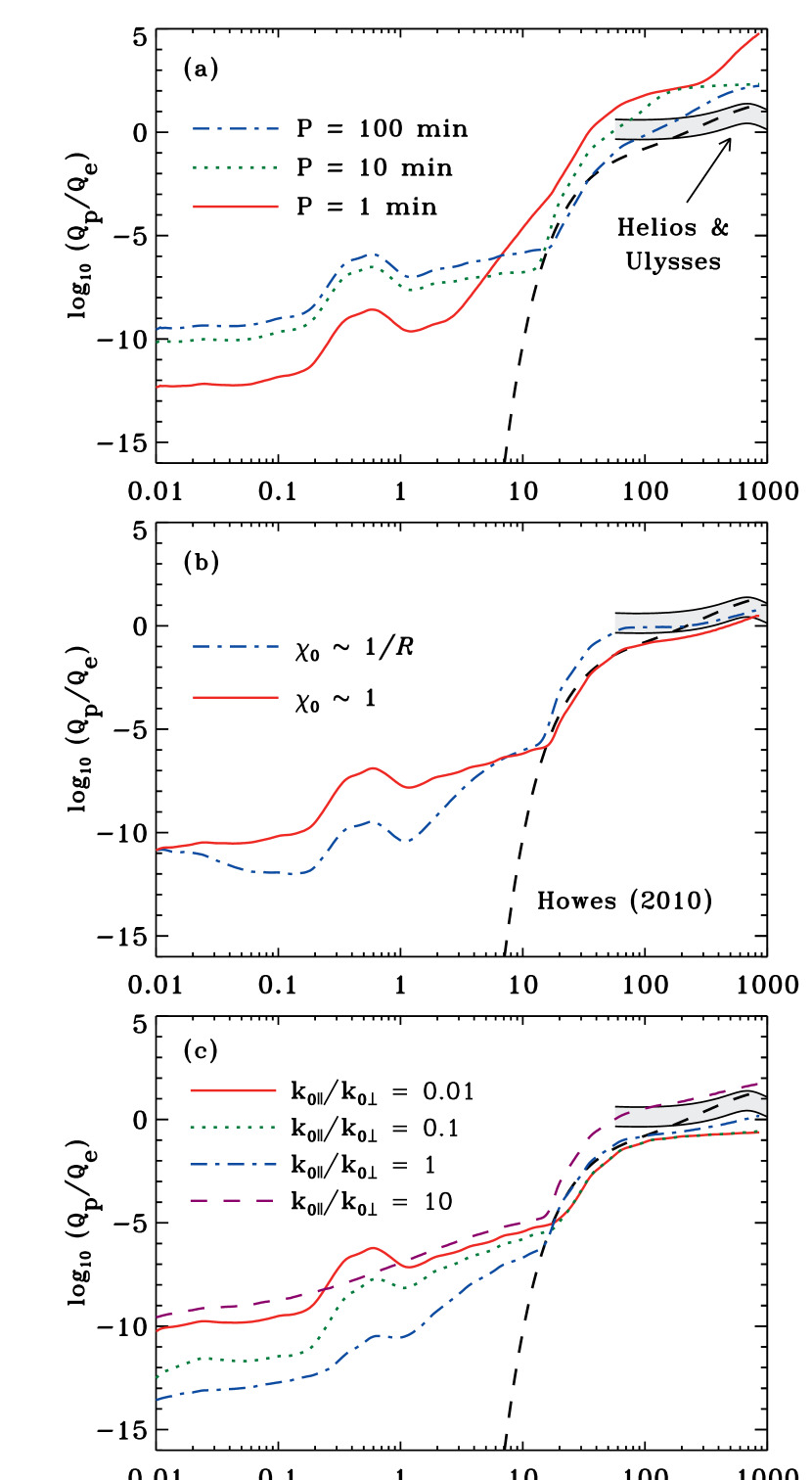
Figure 14.— Radial dependence of $\log Q_{p}/Q_{e}$ for: (a) constant Alfvén wave periods $P=1$ min (solid red curve), $P=10$ min (green dotted curve), and $P=100$ min (blue dot-dashed curve); (b) outer-scale $k_{0\parallel}$ determined from ideal Goldreich & Sridhar (1995) critical balance (red solid curve) and from modified Beresnyak & Lazarian (2008, 2009) critical balance (blue dot-dashed curve); (c) constant ratios $k_{0\parallel}/k_{0\perp}=0.01$ (red solid curve), $k_{0\parallel}/k_{0\perp}=0.1$ (green dotted curve), $k_{0\parallel}/k_{0\perp}=1$ (blue dot-dashed curve), and $k_{0\parallel}/k_{0\perp}=10$ (purple dashed curve). Also shown in (a)–(c) are the Cranmer et al. (2009) measurements (gray region) and the Howes (2010) model prediction (black dashed curve).

In Figure 14 we show the radial dependence of $Q_{p}/Q_{e}$ for various methods of computing the outer-scale parallel wavenumber $k_{0\parallel}$. In all panels, the turbulence spectra were computed with constant values of $s=2$ and $\Phi=0$, as well as the other default parameter choices discussed in Section 3.1. Figure 14(a) assumes a range of radially constant wave frequencies which determine $k_{0\parallel}$ from Equation (43). Figure 14(b) applies the Goldreich & Sridhar (1995) conditions of critical balance for both zero and nonzero cross helicity at the outer scale; see Equations (44)–(45).

Figure 14(c) shows the relative heating rates $Q_{p}/Q_{e}$ for a range of constant ratios $k_{0\parallel}/k_{0\perp}$. At the coronal base ($z=0.01\,R_{\odot}$), note that $Q_{p}/Q_{e}$ behaves non-monotonically as a function of this wavenumber anisotropy ratio. The minimum value of $Q_{p}/Q_{e}$ occurs at $k_{0\parallel}/k_{0\perp}\approx 0.55$. The non-monotonic behavior occurs because of two competing effects. At large values of $k_{0\parallel}$, the weak-turbulence critical balance curve ($\chi_{0}=1$) begins to approach the ion cyclotron frequencies. This has the result of increasing $Q_{p}$ while leaving $Q_{e}$ unchanged. However, when $k_{0\parallel}$ becomes very small, the wave power becomes concentrated into narrower “cones” that provide more energy to the KAWs. This has the result of increasing both $Q_{p}$ and $Q_{e}$, but the smaller rate $Q_{p}$ receives a larger fractional change.

Each panel of Figure 14 also shows the empirically determined range of $Q_{p}/Q_{e}$ ratios from the Helios and Ulysses measurements described by Cranmer et al. (2009). The plotted error range of $\pm 0.3$ in $\log(Q_{p}/Q_{e})$ accounts for both modeling and observational uncertainties. Also, we show the theoretical prediction for $Q_{p}/Q_{e}$ from the gyrokinetic model of Howes (2010) as a dashed black curve. As discussed by Howes (2011), this model agrees well with the Cranmer et al. (2009) measurements at $r\gtrsim 200\,R_{\odot}$, but underestimates the proton heating at $r\lesssim 100\,R_{\odot}$. The Howes (2010) gyrokinetic model includes the same sources of high-$k_{\perp}$ KAW damping that we use, but not the high-$k_{\parallel}$ sources of ion cyclotron damping. In Figure 14, we find that the best agreement with the Cranmer et al. (2009) measured ratio comes from the model that assumes critical balance with the Beresnyak & Lazarian (2008, 2009) modification for nonzero cross helicity; i.e., $\chi_{0}\approx 1/{\cal R}$.

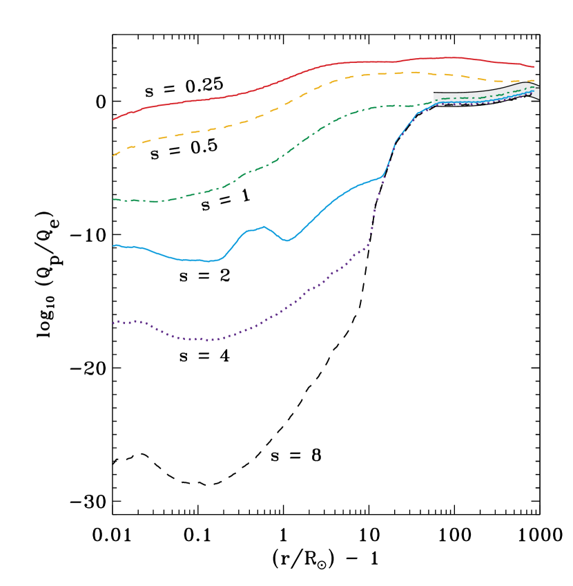
Figure 15.— Radial dependence of $\log Q_{p}/Q_{e}$ for $\chi_{0}\approx 1/{\cal R}$ and $s=0.25$ (red solid curve), $s=0.5$ (orange dashed curve), $s=1$ (green dot-dashed curve), $s=2$ (cyan solid curve), $s=4$ (dark blue dotted curve), and $s=8$ (black dashed curve). Also shown are the Cranmer et al. (2009) measurements (gray region).

In Figure 15 we vary the ratio $s$ used in the Alfvénic parallel cascade function $g(\chi)$; see Equation (C14). We retain the $\chi_{0}\approx 1/{\cal R}$ approximation for $k_{0\parallel}$ that was found to be an optimal choice for agreement with observations at $r\gtrsim 60\,R_{\odot}$. For lower heights in the low-$\beta$ corona, we find that large values of $s$ give insufficient wave power at the ion cyclotron resonant values of $k_{\parallel}$ to provide significant energy to the protons. One would need to specify $s\lesssim 0.5$ in order for there to be enough high-$k_{\parallel}$ power to give protons a substantial fraction of the dissipated energy. Cranmer & van Ballegooijen (2003) and Landi & Cranmer (2009) came to this same essential conclusion. Although there are still no firm experimental or theoretical bounds on the expected value of $s$ in MHD turbulence, it is generally believed that values as low as $s\lesssim 0.5$ are unrealistic.

Figure 16 shows the results of mode coupling between the Alfvén and fast-mode fluctuations. The curves in Figure 16(a) were computed for a range of constant values of the coupling constant $\Phi$ from $10^{-6}$ to $10^{+3}$. At large distances ($r\gtrsim 0.3$ AU), it is clear that the presence or absence of coupling has very little effect on the $Q_{p}/Q_{e}$ ratio. This insensitivity occurs because much of the proton heating at intermediate and high values of $\beta$ comes from the Landau and transit-time damping of KAWs. The low-k_∥, high-$k_{\perp}$ part of the $E_{\rm A}$ spectrum is there no matter the value of $\Phi$, and it dominates the proton and electron heating in this case. The results are similar to those of Howes (2010, 2011) who did not include mode coupling.

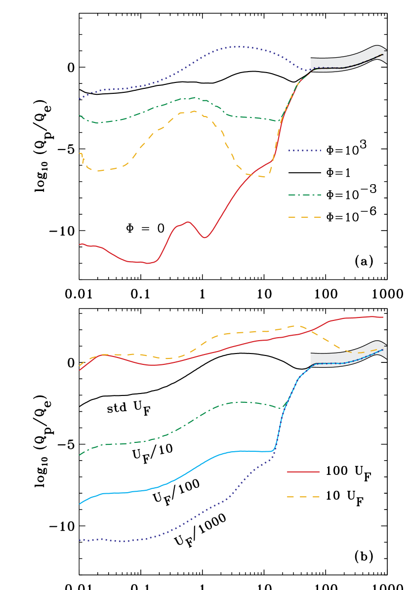
Figure 16.— Radial dependence of $\log Q_{p}/Q_{e}$ for varying properties of Alfvén/fast mode coupling, with: (a) standard model for $U_{\rm F}$ and a range of coupling constants: $\Phi=0$ (red solid curve), $\Phi=10^{-6}$ (orange dashed curve), $\Phi=10^{-3}$ (green dot-dashed curve), $\Phi=1$ (black solid curve), $\Phi=10^{3}$ (dark blue dotted curve); (b) constant value of $\Phi=10$ and a range of modified values for fast-mode power: $U_{\rm F}/10^{3}$ (dark blue dotted curve), $U_{\rm F}/10^{2}$ (cyan solid curve), $U_{\rm F}/10$ (green dot-dashed curve), the standard model of $U_{\rm F}$ (black solid curve), $10U_{\rm F}$ (orange dashed curve), $100U_{\rm F}$ (solid red curve). Also shown in both panels are the Cranmer et al. (2009) measurements (gray regions).

In the low-$\beta$ corona, Figure 16 indicates that $\Phi$ needs to be at least of order unity to excite sufficient power in high-$k_{\parallel}$ ion cyclotron waves to heat protons on par with the electrons (i.e., $Q_{p}/Q_{e}\sim 1$). For low values of $\Phi$, the plotted ratio undergoes several increases and decreases as a function of radius that we cannot trace to any one simple cause. The local maximum that appears at $z\approx 0.5\,R_{\odot}$ corresponds to the local minimum in plasma $\beta$ (see Figure 1). In the low-$\beta$ regime, it is likely that the relative “competition” between mode coupling, transit-time damping (for $E_{\rm F}$), and ion cyclotron damping (for $E_{\rm A}$) undergoes numerous reversals as a function of radius.

In Figure 16(b) we fix the coupling constant at $\Phi=10$, which is of the same order of magnitude as predicted by Chandran (2005), and we vary the normalization of the fast-mode wave power. It was evident from Figure 4 that small changes in the large-scale wave transport properties could give rise to large changes in the fast-mode power in much of the corona and solar wind. Thus, we take the standard model for $U_{\rm F}(r)$ and multiply it by constant factors ranging from $10^{-3}$ to $10^{+2}$. We note, however, that we do not have excessive freedom to increase the $U_{\rm F}$ normalization too far above the standard model. A significantly higher coronal population of fast-mode waves would contribute to a larger $v_{\perp}$ that may exceed the observational constraints shown in Figure 3(a). Nonetheless, Figure 16(b) shows that the standard model ends up being a reasonable solution that matches the observed in situ heating ratio (Cranmer et al., 2009) and also gives appreciable proton heating in the extended corona (as required qualitatively from UVCS proton temperature measurements); see Cranmer & van Ballegooijen (2003).

An example calculation of preferential heavy ion heating is shown in Figure 17. The ion used for the model was O⁺⁵, whose properties have been measured in the corona from emission in the O VI 1032, 1037 Å spectral line doublet (Kohl et al., 2006). We used the parameters corresponding to the best agreement with observational constraints on $Q_{p}/Q_{e}$ (see Table 2). We then adjusted the fast-mode wave power $U_{\rm F}(r)$ by changing the multiplicative constant that was varied in Figure 16(b). As in Figure 16(b), values of this multiplicative constant between about 1 and 10 appear to bracket the observational constraints.

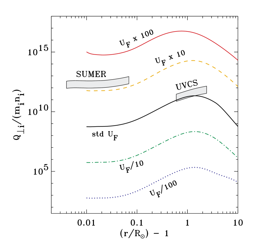
Figure 17.— Radial dependence of the perpendicular heating rate per unit mass $Q_{\perp i}/(m_{i}n_{i})$, in units of erg s^-1 g^-1, for O⁺⁵ ions. Model results shown for a range of modified values for fast-mode power: $U_{\rm F}/100$ (dark blue dotted curve), $U_{\rm F}/10$ (green dot-dashed curve), standard $U_{\rm F}$ (black solid curve), $10U_{\rm F}$ (orange dashed curve), $100U_{\rm F}$ (solid red curve). Also shown are empirical constraints from SUMER and UVCS emission line measurements (gray regions).

The plotted ranges for the observationally determined $Q_{\perp i}$ rates were derived by combining observations from both the UVCS (Cranmer et al., 1999) and SUMER (Landi & Cranmer, 2009) instruments on SOHO with semi-empirical solutions of the perpendicular internal energy conservation equations. These heating rates were not given explicitly by either Cranmer et al. (1999) or Landi & Cranmer (2009), but they were computed and saved from the models that produced agreement with the observed radial behavior of $T_{\perp i}$. The SUMER and UVCS data were obtained for off-limb measurements of O VI emission, in which the line widths are primary diagnostics of $T_{\perp i}$. Note that the radial dependence of the two observationally determined regions is similar to that in the plotted model curves. However, the SUMER data corresponds to about a factor of 10 higher fast-mode wave power normalization than the UVCS data.

If the postulated mode-coupling explanation for ion cyclotron proton/ion heating is correct, then the results given in Figures 16 and 17 constrain the required levels of fast-mode wave power. In the low corona ($z\lesssim 0.1\,R_{\odot}$), there may need to be up to a factor of 10 higher value of $U_{\rm F}$ than in the standard model of Section 2, but in the extended corona and heliosphere the standard model may be close to correct. Of course, it is only the high-$k_{\parallel}$ tail of the fast-mode spectrum that matters to the calculation of available Alfvénic power at the ion cyclotron resonances, not its outer-scale normalization. Therefore it is possible that $U_{\rm F}$ may depart significantly from the values predicted by the standard model of Section 2, but still produce agreement with the various observations by having different values for the spectral slope and angle-dependence of $E_{\rm F}({\bf k})$.

7. Discussion and Conclusions

The aim of this paper was to explore the consequences of Chandran’s (2005) conjecture that nonlinear couplings between Alfvén and fast-mode waves may produce sufficient ion cyclotron wave power to heat protons and heavy ions in the corona. To test this idea, we constructed a semi-empirical model of the background plasma and MHD wave properties in a flux tube connected to a polar coronal hole. For the sake of practicality, we utilized several approximations when solving the wave energy transport equations for the energy densities of Alfvén, fast, and slow modes:

1. The equations themselves were adapted from standard WKB “wave action conservation” theory, which does not take account of the effects of linear wave reflection in a fully self-consistent manner. We also assumed the associated WKB limiting case of equipartition between the kinetic and magnetic energy densities for the dominant Alfvén waves (i.e., $K_{y}=M_{y}$). Roughly speaking, these approximations are consistent with an assumption that the wave frequencies are higher than $\sim 10^{-3}$ Hz in the corona. However, it has also been shown that the radial behavior of Alfvénic wave power in the solar wind is never far from the predictions of WKB theory even in the heliosphere where reflection is not negligible (Zank et al., 1996; Cranmer & van Ballegooijen, 2005).

2. Because of other evidence that the dominant inertial-frame frequencies in coronal MHD turbulence may be lower than $\sim 10^{-4}$ Hz (see, e.g., Chandran & Hollweg, 2009; Cranmer, 2010), we made use of a low-frequency approximation for the Alfvén wave reflection coefficient ${\cal R}$. This also involved an analytic approximation for the radial dependence of the Alfvén speed scale height $H_{\rm A}$ (Equation (25)).

3. For the fast and slow magnetosonic waves, we modeled the radial transport of an isotropic ensemble of propagation directions $\theta$ using a single wave action conservation equation. We chose one reasonable method to perform the averages over $\theta$, but other methods may yield different results. We also used the Eulerian average for the outflow speed $u_{0}$ and neglected the second-order effects of “Stokes drift” that would enter into the associated Lagrangian version of the mean (see Cranmer, 2009b).

Although the effects of removing these approximations should be investigated further, we do not believe their use invalidates the results of the wave transport models presented above.

With the above caveats taken into account, we produced a standard model of the Alfvén, fast, and slow mode energy densities between 0.01 and 1000 $R_{\odot}$ above the solar photosphere. In agreement with earlier results, we found that slow-mode MHD waves of solar origin probably cannot survive into the extended corona. In addition, we found that the amplitudes of fast-mode waves at large distances are more sensitive to the assumed model parameters than are the amplitudes of Alfvén waves. For this reason the standard model of fast-mode wave energy density was treated as a representative example and not a definitive prediction. Thus, other reasonable models of the available fast-mode power can be obtained by multiplying or dividing the standard model’s energy density by factors of order 10–100 without sacrificing too much realism.

At each radial distance, we simulated the time-steady wavenumber power spectra of Alfvénic and fast-mode turbulent fluctuations. We included the effects of nonlinear coupling and collisionless kinetic wave dissipation. We also computed the time-steady heating rates for protons, electrons, and a representative minor ion species (O⁺⁵) for comparison with observational constraints. The resulting heating rates for the standard model of fast-mode wave power was found to provide both substantial heating for coronal protons as well as produce agreement with the preferential O⁺⁵ ion heating measured by UVCS/SOHO. However, if the fast-mode wave power in the corona is significantly lower than was assumed in the standard model, the proposed idea of mode coupling is probably not a viable mechanism for the ion heating.

In order to match some of the observations—such as the need for $Q_{p}/Q_{e}$ to be of order unity at $z\lesssim 0.1\,R_{\odot}$ and for the O⁺⁵ heating rate to agree with that measured by SUMER/SOHO at similar heights—we found that approximately 10 times the standard model’s assumed fast-mode wave energy density may need to be present. This could be accounted for in several ways. First, we neglected the effects of Alfvén waves giving rise to second order fluctuations that mimic the properties of both fast and slow magnetosonic waves (Hollweg, 1971; Vasquez & Hollweg, 1999). It is possible that these secondary oscillations could behave similarly enough to ideal fast-mode waves that they enable the same kinds of cascade and coupling. Second, we also neglected nonlinear couplings that involve slow-mode MHD waves, which appear to dominate the density fluctuations in the low corona. It may be possible for these couplings (see, e.g., Yoon & Fang, 2008) to also power the high-$k_{\parallel}$ part of the Alfvénic fluctuation spectrum.

To make further progress with the proposed set of ideas, it will be important to better understand the origin of the fast, slow, and Alfvén waves in the solar photosphere and chromosphere. Hollweg (1978a), Spruit (1981), and others studied the wavelike oscillations induced by convective jostling in small-scale flux tubes that extend up into the chromosphere. However, once waves reach the sharp and “corrugated” TR boundary, they can undergo reflection, refraction, and multiple types of mode conversion (Hollweg, 1978b; Bogdan et al., 2002; Hasan & van Ballegooijen, 2008; Fedun et al., 2011; Cally & Hansen, 2011). The types and strengths of MHD waves that survive the chaotic lower atmosphere probably also depend on the nature of the region underlying the solar wind flux tubes of interest (i.e., coronal hole, active region, or quiet loops).

Future work must also involve more physical realism for the model of turbulent cascade. Replacing our hodge-podge collection of analytic solutions with a fully self-consistent numerical simulation is an obvious priority. A key part of this improvement will be to remove the assumption of scale separation that prevents different radial zones from interacting with one another in wavenumber space (see, e.g., Verdini et al., 2009). In addition, we note that the advection-diffusion terms in Equations (31)–(32) contain the limiting assumption that the spectral transfer is “local” in ${\bf k}$-space. It has been shown that true MHD turbulence is not so local because of intermittent high-order wave-wave interactions and nonlinear steepening effects (e.g., Medvedev, 2000; Chandran, 2008b; Cho, 2010; Howes et al., 2012). We also assumed energy equipartition between the $v_{\perp}$ and $b_{\perp}$ spectra in the MHD inertial range, but in situ measurements show that not to be the case in actual solar wind turbulence (Grappin et al., 1983; Wang et al., 2011).

We also intend to improve upon the kinetic treatment of collisionless particle heating described in Section 5. We assumed isotropic Maxwellian velocity distributions when solving for the linear damping rates, but Bashir et al. (2010) showed how non-Maxwellian temperature anisotropies can significantly affect the KAW dispersion relation. The ultimate rate of electron heating from KAW Landau damping can also be affected by nonlinearity and Coulomb collision effects that we did not include (e.g., Borovsky & Gary, 2011). The time evolution of proton and ion velocity distributions, under the influence of cyclotron resonant heating, is also decidedly non-Maxwellian (Galinsky & Shevchenko, 2000; Isenberg, 2001; Cranmer, 2001; Isenberg & Vasquez, 2009, 2011).

Finally, we emphasize that the proposed idea of nonlinear coupling between Alfvén and fast-mode waves is only one proposed solution to the problem of preferential proton/ion heating. Some of the other suggested explanations were listed briefly in Section 1. One recent example that has received significant attention is the stochastic energization of protons and ions that occurs when KAW amplitudes become sufficiently high (Johnson & Cheng, 2001; Chandran, 2010; Chandran et al., 2011). To excite this proposed stochasticity, the dimensionless ratio $v_{\perp}/c_{s}$ (evaluated at $k_{\perp}\rho_{p}=1$) should exceed values of order 0.1. However, in this paper’s standard model of Alfvénic fluctuations (either with or without nonlinear couplings), this ratio never exceeds a value of 0.003. The main factor responsible for this dramatic mismatch is our assumption of the Goldreich & Sridhar (1995) scaling in the limit of strong turbulence (i.e., $v_{\perp}\propto k_{\perp}^{-1/3}$). Alternate theories of the strong Alfvénic cascade (e.g., Boldyrev, 2006; Podesta, 2011) give a shallower dependence of $v_{\perp}\propto k_{\perp}^{-1/4}$. This would allow larger values of $v_{\perp}$ to survive to the onset of KAW dispersion at $k_{\perp}\rho_{p}\approx 1$. We await improved theoretical descriptions of MHD turbulence and conclusive empirical tests of such models.

Appendix A A. Heuristic Overview of MHD Turbulence

The cascade of energy from large to small eddies was first described in the context of isotropic hydrodynamic turbulence (von Kármán & Howarth, 1938; Kolmogorov, 1941; Obukhov, 1941; Batchelor, 1953). The spectral transport timescale for energy to be transferred down to the next order of magnitude of eddy size is estimated generally as $\tau_{s}\approx(kv_{k})^{-1}$, where $k$ is the magnitude of the local wavevector ${\bf k}$ and $v_{k}$ is the local eddy velocity at this value of $k$. For isotropic fluctuations that depend only on $k$ and not its direction, we can define the reduced one-dimensional spectrum $e_{m}(k)=v_{k}^{2}/k$. Thus, since

$$\frac{U_{m}}{\rho_{0}}\,=\,\int dk\,\,e_{m}(k)\,\,,$$ (A1)

we relate the eddy velocity to the full three-dimensional spectrum via $v_{k}^{2}=4\pi k^{3}E_{m}$. The cascade rate is estimated as $\varepsilon\sim v_{k}^{2}/\tau_{s}$. Assuming that $\varepsilon$ is constant in the inertial range leads to the time-steady Kolmogorov-Obukhov spectrum $e_{m}\propto k^{-5/3}$, or $E_{m}\propto k^{-11/3}$.

When the background magnetic field becomes strong, other physical processes become important. Iroshnikov (1963) and Kraichnan (1965) (hereafter IK) realized that the “eddy” description of hydrodynamic turbulence could be generalized by referring to colliding MHD wave packets, and that the Alfvén speed $V_{\rm A}$ introduces a new absolute scale into the problem. If one continues to treat the cascade isotropically in $k$-space, a more generalized spectral transport time can be defined as

$$\tau_{s}\,=\,\frac{1}{kv_{k}}\left(\frac{V_{\rm A}}{v_{k}}\right)^{p}$$ (A2)

where $p=0$ gives the Kolmogorov-Obukhov limit and $p=1$ is the result of the IK analysis. Using the same assumption above that $\varepsilon$ is constant, we obtain a more general one-dimensional power spectrum $e_{m}\propto k^{-(p+5)/(p+3)}$. For the IK value of $p=1$, the spectrum is $e_{m}\propto k^{-3/2}$ (see also Boldyrev, 2005).

It has been known for several decades that a cascade of Alfvén-wave-like fluctuations does not lead to an isotropic distribution of power in wavenumber space (Strauss, 1976; Montgomery & Turner, 1981; Shebalin et al., 1983; Higdon, 1984). The dominant energy cascade takes place mainly in the two-dimensional plane perpendicular to the background field. For the Alfvénic fluctuations, we can define the local eddy velocity as $v_{\perp}$ being mainly a function of $k_{\perp}$. The one-dimensional spectrum in this case is given by $e_{\rm A}=v_{\perp}^{2}/k_{\perp}$ and the integration over wavenumber space is best done in cylindrical coordinates with

$$\frac{U_{\rm A}}{2\pi\rho_{0}}\,=\,\int dk_{\parallel}\int dk_{\perp}\,k_{\perp}E_{\rm A}\,=\,\int dk_{\perp}\,e_{\rm A}\,\,.$$ (A3)

Taking into account the spectral anisotropy ($k_{\parallel}\neq k_{\perp}$) we can also write an even more general perpendicular transport time for the Alfvén waves as

$$\tau_{\rm A}\,=\,\frac{1}{k_{\perp}v_{\perp}}\left(\frac{V_{\rm A}}{v_{\perp}}\right)^{p}\left(\frac{k_{\parallel}}{k_{\perp}}\right)^{q}\,\,.$$ (A4)

A perpendicular generalization of the IK model is given by $p=1$ and $q=0$, which gives $e_{\rm A}\propto k_{\perp}^{-3/2}$ (see also Nakayama, 1999, 2001; Boldyrev, 2006; Podesta, 2011). Weak three-wave couplings have been shown to give rise to the case $p=q=1$, which yields $e_{\rm A}\propto k_{\perp}^{-2}$ (e.g., Galtier et al., 2000; Bhattacharjee & Ng, 2001; Boldyrev & Perez, 2009). However, in that case nonlinear effects grow in magnitude as $k_{\perp}$ gets larger, so it is generally believed that a weakly turbulent inertial range must eventually become strongly turbulent (see also Goldreich & Sridhar, 1997).

Goldreich & Sridhar (1995) described strong Alfvénic turbulence with a spectral transfer time given by $p=q=0$, and thus $e_{\rm A}\propto k_{\perp}^{-5/3}$ reminiscent of the original Kolmogorov-Obukhov model. In this case of strong mixing between the turbulent motions (perpendicular to the field) and the flow of Alfvén wave packets (parallel to the field) there is a so-called “critical balance” that couples $k_{\perp}$ and $k_{\parallel}$ to one another. We define a critical balance parameter

$$\chi\,\approx\,\frac{k_{\parallel}V_{\rm A}}{k_{\perp}v_{\perp}}$$ (A5)

such that the Goldreich & Sridhar (1995) strong cascade is consistent with the condition $\chi\approx 1$. Combining this with the velocity scaling $v_{\perp}\propto k_{\perp}^{-1/3}$ yields the wavenumber anisotropy scaling $k_{\parallel}\propto k_{\perp}^{2/3}$. Note that assuming $p=q$ in Equation (A4) is equivalent to $\tau_{\rm A}$ being given by $\chi^{p}/(k_{\perp}v_{\perp})$; see also Galtier et al. (2005). An alternate way of describing the cascade was given by Zhou & Matthaeus (1990b), who defined a triple correlation timescale equivalent to

$$\tau_{\rm A}\,\approx\,\frac{1+\chi}{k_{\perp}v_{\perp}}\,\,.$$ (A6)

This expression naturally bridges the strong ($\chi\lesssim 1$) and weak ($\chi\gg 1$) turbulence scaling limits, and we use a similar relation in Section 3.1.

The cascade of compressible fast-mode waves has received less attention than that of the incompressible Alfvén waves. Because fast-mode waves propagate at a roughly constant phase speed no matter the direction angle $\theta$, the fast-mode cascade has been suspected to resemble isotropic hydrodynamic turbulence. In fact, numerical simulations do tend to find that fast-mode waves produce a more isotropic spectrum than do Alfvén waves (Cho & Lazarian, 2003; Svidzinski et al., 2009). The rate of the cascade is generally assumed to follow the weak IK-type scaling of Equation (A2) with $p=1$ (see, e.g., Chandran, 2005; Suzuki et al., 2007). Thus, because in most cases we expect $v_{k}\ll V_{\rm A}$, the fast-mode cascade timescale $\tau_{\rm F}$ is likely to be significantly longer than the Alfvénic timescale $\tau_{\rm A}$.

It is important to emphasize that there is still no agreement concerning the most realistic and universal way to describe MHD turbulence. There remains controversy about the applicability of the various power law exponents (especially $5/3$ versus $3/2$) for the Alfvénic inertial range (Beresnyak, 2011; Forman et al., 2011; Mason et al., 2011; Podesta, 2011). Simulations have not been able to accurately pin down the amount of slow “leakage” of power to the high-$k_{\parallel}$ region of the spectrum where $\chi\gg 1$. Furthermore, the observed steepening of the spectrum at high values of $k_{\perp}$ is still not well understood (Leamon et al., 1998; Stawicki et al., 2001; Howes et al., 2008). In many models, the precise scalings depend on the degree of cross helicity of the fluctuations (i.e., on the imbalance between $Z_{+}$ and $Z_{-}$) and on whether the turbulence is driven or decaying (e.g., Lithwick et al., 2007; Chandran, 2008b; Chen et al., 2011). In this paper, we attempt to identify the most controversial aspects of the models and discuss how they can be modified once such issues are resolved.

Appendix B B. Linear Damping Rates: Collisional and Collisionless

Alfvén (1947) and Osterbrock (1961) first proposed that MHD waves in the solar atmosphere could be damped by collisional processes. These processes include viscosity, thermal conductivity, electrical resistivity (i.e., Joule or Ohmic dissipation), and ion-neutral friction. In the fully collisional regime we make use of the basic expressions derived by Braginskii (1965). Here we describe the total linear damping rate for MHD wave mode $m$ by a sum of three components,

$$\gamma_{m}\,=\,\gamma_{{\rm vis,}m}+\gamma_{{\rm ohm,}m}+\gamma_{{\rm con,}m}$$ (B1)

where $\gamma_{{\rm vis,}m}$ denotes damping due to kinematic viscosity, $\gamma_{{\rm ohm,}m}$ denotes electrical resistivity, and $\gamma_{{\rm con,}m}$ denotes thermal conductivity. Since our main goal is to model the wave damping in the (almost completely ionized) corona and solar wind, we ignore ion-neutral friction. For Alfvén waves,

$$\gamma_{\rm vis,A}\,=\,\frac{1}{\rho_{0}}\left(\eta_{1}\,k_{\perp}^{2}+\eta_{2}\,k_{\parallel}^{2}\right)$$ (B2)

$$\gamma_{\rm ohm,A}\,=\,\left(\frac{c^{2}}{4\pi\sigma_{\parallel}}\right)k_{\perp}^{2}+\left(\frac{c^{2}}{4\pi\sigma_{\perp}}\right)k_{\parallel}^{2}$$ (B3)

$$\gamma_{\rm con,A}\,=\,0\,\,.$$ (B4)

For fast and slow mode waves ($m=\mbox{F,S}$), we note that the damping rates given explicitly by Braginskii (1965) are valid only in the $\beta\ll 1$ limit. The expressions given here are appropriate for arbitrary values of $\beta$, but we made the assumption that $k_{\parallel}\approx k_{\perp}$. In other words, for the assumed isotropic distribution of fast and slow wave vectors, the damping rates depend only on the magnitude $k^{2}=k_{\parallel}^{2}+k_{\perp}^{2}$. With that caveat, the damping rates are given by

$$\gamma_{{\rm vis,}m}\,=\,\frac{2k^{2}}{\rho_{0}}\left[\frac{\eta_{0}}{3}\left(4f_{vz}-4f_{xz}+f_{vx}\right)+\eta_{1}f_{vx}+\eta_{2}\left(f_{vx}+2f_{xz}+f_{vz}\right)\right]$$ (B5)

$$\gamma_{{\rm ohm,}m}\,=\,\frac{c^{2}k^{2}f_{\rm B}}{4\pi\sigma_{\perp}}$$ (B6)

$$\gamma_{{\rm con,}m}\,=\,\frac{4(\gamma-1)^{2}k_{\rm B}T}{\rho_{0}c_{s}^{2}}\,f_{\rm th}k^{2}\left(\kappa_{\parallel}+\kappa_{\perp}\right)\,\,,$$ (B7)

where the fractions $f$ specify the energy partition fractions of Section 2.2. Specifically, $f_{\rm th}=\Theta/U_{m}$, $f_{\rm B}=(M_{x}+M_{z})/U_{m}$, $f_{vx}=K_{x}/U_{m}$, $f_{vz}=K_{z}/U_{m}$, and $f_{xz}=(f_{vx}f_{vz})^{1/2}$. We assume that protons dominate other ion species in the viscosity and thermal conductivity terms, and that electrons dominate the electrical resistivity terms (see also Tu, 1984; Whang, 1997; Campos, 1999).

We use the Braginskii (1965) expressions for the transport coefficients in the fully collisional limit. These coefficients depend on the proton and electron Coulomb collision timescales (e.g., Spitzer, 1962),

$$\tau_{p}\,=\,\frac{3}{4}\sqrt{\frac{m_{p}}{\pi}}\frac{(k_{\rm B}T_{p})^{3/2}}{e^{4}n_{p}\ln\Lambda}$$ (B8)

$$\tau_{e}\,=\,\frac{3}{4}\sqrt{\frac{m_{e}}{2\pi}}\frac{(k_{\rm B}T_{e})^{3/2}}{e^{4}n_{p}\ln\Lambda}$$ (B9)

where we approximate the Coulomb logarithm in the coronal regime of temperatures and densities by

$$\ln\Lambda\,=\,23.2+\frac{3}{2}\ln\left(\frac{T_{e}}{10^{6}\,\mbox{K}}\right)-\frac{1}{2}\ln\left(\frac{n_{e}}{10^{6}\,\mbox{cm}^{-3}}\right)\,\,.$$ (B10)

We also specify the magnitudes of the proton and electron gyrofrequencies,

$$\Omega_{p}=\frac{eB_{0}}{m_{p}c}\,\,,\,\,\,\,\Omega_{e}=\frac{eB_{0}}{m_{e}c}$$ (B11)

and the dimensionless products

$$x_{p}=\tau_{p}\Omega_{p}\,\,,\,\,\,\,x_{e}=\tau_{e}\Omega_{e}\,\,.$$ (B12)

Thus, the proton viscosity coefficients are given by

$$\eta_{0}=0.96\,n_{p}k_{\rm B}T_{p}\tau_{p}\,\,,\,\,\,\,\eta_{1}=2x_{p}\eta_{2}$$ (B13)

$$\eta_{2}=n_{p}k_{\rm B}T_{p}\tau_{p}\left(\frac{1.2x_{p}^{2}+2.23}{x_{p}^{4}+4.03x_{p}^{2}+2.33}\right)\,\,.$$ (B14)

The electrical conductivities are given by

$$\sigma_{\parallel}=\frac{1.95\,e^{2}n_{e}\tau_{e}}{m_{e}}$$ (B15)

$$\sigma_{\perp}=\frac{e^{2}n_{e}\tau_{e}}{m_{e}}\left(1-\frac{6.416x_{e}^{2}+1.837}{x_{e}^{4}+14.79x_{e}^{2}+3.7703}\right)^{-1}\,\,.$$ (B16)

The thermal conductivities are given by

$$\kappa_{\parallel}=\frac{3.906\,n_{p}k_{\rm B}T_{p}\tau_{p}}{m_{p}}$$ (B17)

$$\kappa_{\perp}=\frac{n_{p}k_{\rm B}T_{p}\tau_{p}}{m_{p}}\left(\frac{2x_{p}^{2}+2.645}{x_{p}^{4}+2.70x_{p}^{2}+0.677}\right)\,\,.$$ (B18)

Finally, we need to take account of the transition from collisional to collisionless wave damping. In the low-density limit of the classical Braginskii (1965) expressions, some of the transport coefficients (e.g., $\eta_{0}$, $\eta_{1}$, $\kappa_{\parallel}$) become infinitely large as the mean time between collisions becomes infinite. This “molasses limit” has been recognized to be unphysical (see Williams, 1995; Cranmer & van Ballegooijen, 2005). Thus, we derived a simplified version of the general expressions of Chang & Callen (1992) and Ji et al. (2009) to describe what happens when collisions become infrequent. We computed the $\gamma$ dissipation rates as above, but then we multiplied them all by the following dimensionless factor $C$, where

$$C=\frac{\tau_{\rm esc}}{\tau_{\rm esc}+\tau_{p}}$$ (B19)

and the macroscopic expansion timescale for waves is estimated as

$$\tau_{\rm esc}\approx\frac{\rho_{0}}{(u+V_{\rm A})|\partial\rho_{0}/\partial r|}\,\,.$$ (B20)

For strong collisions, $C\approx 1$ and the Braginskii (1965) expressions are valid. For weak collisions, $C\approx\tau_{\rm esc}/\tau_{p}\ll 1$ and the damping rates are quenched.

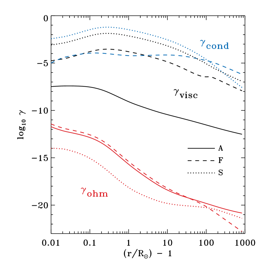
Figure 18.— Linear collisional damping rates for MHD waves. Color denotes the physical dissipation process: viscosity (black), electrical resistivity (red), and thermal conductivity (blue). Line style denotes the wave mode: Alfvén (solid curves), fast mode (dashed curves), and slow mode (dotted curves). All quantities are plotted as base-10 logarithms of the rates, in units of s^-1, for the standard model with parameters listed in Table 1.

Figure 18 illustrates how the components of the wave damping rates vary with radial distance in the model of the fast solar wind described in Section 2. For the fast and slow mode waves, the viscous and conductive damping terms are of roughly comparable strength, but for the fast mode the conductive damping wins out at large distances ($\beta\gg 1$). The viscous term is most important for the Alfvén mode, but its magnitude remains small in comparison to the dominant terms for fast and slow mode damping. At the heights displayed here, Ohmic dissipation never appears to be important in comparison to the other terms. This situation is reversed, however, lower down in the chromosphere (see, e.g., Khodachenko et al., 2004). The curves in Figure 18 are shown for the general case of the transition to a collisionless plasma (i.e., with all rates multiplied by $C$). For $z\lesssim 0.1\,R_{\odot}$ in the low corona, $C\approx 1$ and the general rates are identical to the unmodified Braginskii (1965) rates. For heights greater than $z\approx 1\,R_{\odot}$, however, the the rates multiplied by $C$ become about two orders of magnitude smaller than the unmodified classical rates.

Appendix C C. Analytic Solutions to Advection-Diffusion Problems in Limited Parameter Regimes

C.1. C.1. Alfvén Waves: Cascade and Source Terms

Equation (38) is a reduced one-dimensional version of the full advection-diffusion equation for Alfvénic fluctuations. The Appendix of Cranmer & van Ballegooijen (2003) presented one method of solving this equation in the low-wavenumber, strong turbulence ($\chi_{0}\ll 1$) limit. Here we derive a more general case for arbitrary $\chi_{0}$. Ignoring both wave damping and mode coupling, and assuming a steady state (i.e., $\partial b_{\perp}^{2}/\partial t=0$), Equation (38) can be simplified to

$$\frac{\partial\varepsilon}{\partial x}\,=\,\tilde{S}_{\rm A}$$ (C1)

where here we define $x=\ln k_{\perp}$ and we write the cascade rate as

$$\varepsilon = \frac{1}{\tau_{\rm A}}\left(\mu_{\perp}b_{\perp}^{2}-\alpha_{\perp}\frac{\partial b_{\perp}^{2}}{\partial x}\right)$$ (C2)

$$= -\frac{\alpha_{\perp}k_{\perp}^{1+s}}{\tau_{\rm A}}\frac{\partial}{\partial k_{\perp}}\left(b_{\perp}^{2}k_{\perp}^{-s}\right)$$ (C3)

where $s=\mu_{\perp}/\alpha_{\perp}$. Note that the ratio $s$ was called $\beta/\gamma$ by Cranmer & van Ballegooijen (2003) and Landi & Cranmer (2009). The second form for $\varepsilon$ given in Equation (C3) helps to show that the power-law spectrum for $b_{\perp}$ in the inertial range (i.e., where $\tilde{S}_{\rm A}=0$ and $\varepsilon$ is constant) should be independent of the value of $s$. In the limiting cases of strong ($\chi_{0}\ll 1$) and weak ($\chi_{0}\gg 1$) turbulence, we use Equation (36) to find that $b_{\perp}$ is proportional to $k_{\perp}^{-1/3}$ and $k_{\perp}^{-1/2}$, respectively.

In regions of wavenumber space where the source term is nonzero, $\varepsilon$ is not constant and the simple inertial-range scalings do not apply. If we assume that most of the fluctuation power is injected near $x\approx x_{0}=\ln k_{0\perp}$, then it makes sense to use a compact Gaussian shape for the source term,

$$\tilde{S}_{\rm A}(x)\,=\,\frac{\varepsilon_{0}}{\pi^{1/2}\sigma_{0}}\exp\left[-\left(\frac{x-x_{0}}{\sigma_{0}}\right)^{2}\right]\,\,,$$ (C4)

where the dimensionless width of the Gaussian is specified by $\sigma_{0}=1$ in our models. The constant $\varepsilon_{0}$ is varied arbitrarily to produce the desired total fluctuation energy density $U_{\rm A}$. Cranmer & van Ballegooijen (2003) showed how the above form for the source function integrates to a cascade rate

$$\varepsilon(x)\,=\,\frac{\varepsilon_{0}}{2}\left[1+\mbox{erf}\left(\frac{x-x_{0}}{\sigma_{0}}\right)\right]\,\,.$$ (C5)

Finally, we define an auxiliary parameter $q=b_{\perp}^{2}k_{\perp}^{-s}$ and integrate Equation (C3) to obtain

$$q^{3/2}\,=\,\frac{3}{2\alpha_{\perp}}\int_{k_{\perp}}^{\infty}\frac{d\kappa\,(1+\chi_{0})\,\varepsilon(\kappa)}{\phi^{1/2}\kappa^{2+(3s/2)}}\,\,.$$ (C6)

In practice, we integrate this equation numerically and use the definition of $q$ to obtain $b_{\perp}(k_{\perp})$. In the energy containing range ($x\ll x_{0}$), we see that $\varepsilon\rightarrow 0$, and thus $q$ is constant and $b_{\perp}^{2}\propto k_{\perp}^{s}$. The low-$k_{\perp}$ region of wavenumber space stands in contrast to the inertial range because here the shape of the fluctuation spectrum does depend on the value of $s$.

In the MHD strong-turbulence inertial range (where $\varepsilon\approx\varepsilon_{0}$, $\phi\approx 1$, and $\chi_{0}\ll 1$), we obtain the standard solution $b_{\perp}\propto v_{\perp}\propto k_{\perp}^{-1/3}$. However, when $k_{\perp}\rho_{p}$ increases past unity into the KAW dispersive range, we see from Equation (35) that for $\beta\gg 1$ there exists a sizable “dispersion range” in which $\phi\propto k_{\perp}^{2}$ and we obtain

$$b_{\perp}\propto k_{\perp}^{-2/3}\,\,,\,\,\,\,v_{\perp}\propto k_{\perp}^{+1/3}\,\,.$$ (C7)

Converting these into the more commonly used one-dimensional spectra (see Appendix A), the MHD inertial range has $e_{\rm A}\propto k_{\perp}^{-5/3}$, and the KAW inertial range has $e_{\rm A}\propto k_{\perp}^{-7/3}$ for the magnetic fluctuations and $e_{\rm A}\propto k_{\perp}^{-1/3}$ for the (electron) velocity fluctuations. These scalings have been described by, e.g., Biskamp et al. (1996), Cranmer & van Ballegooijen (2003), and Howes et al. (2008). Note, however, that strong damping also begins to occur in the KAW regime, so the above power laws may not be evident in the final modeled spectra.

C.2. C.2. Alfvén Waves: Cascade and Dissipation Terms

We include the effects of high-$k_{\perp}$ dissipation in the perpendicular cascade by assuming the damping acts only at wavenumbers significantly above those where the source term is dominant. Thus, we assume that $\tilde{S}_{\rm A}=0$ and we continue to ignore mode coupling. In this limiting case, the time-steady advection-diffusion equation becomes

$$k_{\perp}\frac{\partial\varepsilon}{\partial k_{\perp}}\,=\,-2\tilde{\gamma}_{\rm A}b_{\perp}^{2}\,\,.$$ (C8)

We note that Howes et al. (2008) found it is important to include KAW damping when solving for the steady-state wave power (and thus the proton/electron energy partitioning) at large values of $k_{\perp}$.

In Appendix C.1 we showed that the properties of the inertial range spectra should be independent of the value of $s$. In order to produce a closed-form solution, here we follow Howes et al. (2008) and assume that $s\rightarrow\infty$ (i.e., the cascade proceeds purely by wavenumber advection). Thus, by assuming that $\alpha_{\perp}=0$, we can use Equation (C2) to write the $b_{\perp}^{2}$ term on the right-hand side of Equation (C8) as

$$b_{\perp}^{2}\,\approx\,\frac{\varepsilon}{\mu_{\perp}k_{\perp}v_{\perp}}$$ (C9)

if we also assume $\chi_{0}\ll 1$ in the high-$k_{\perp}$ limit. To retain the most generality in cases when $s$ is not infinitely large, we can use Equation (41) to replace $\mu_{\perp}$ by $\mu_{\perp\ast}=\mu_{\perp}+2\alpha_{\perp}/3$. This may not be completely accurate for the cases of weakest advection (i.e., $s\approx 0$), but it is an improvement on ignoring the influence of the $\alpha_{\perp}$ diffusion term altogether.

To simplify the modified transport equation, we take a further cue from Howes et al. (2008) and use the critical balance condition $\omega\approx k_{\perp}v_{\perp}$ to rewrite the equation as

$$\frac{k_{\perp}}{\varepsilon}\frac{\partial\varepsilon}{\partial k_{\perp}}\,=\,-\frac{2}{\mu_{\perp\ast}}\left(\frac{\tilde{\gamma}}{\omega}\right)_{\rm A}$$ (C10)

where the ratio $(\tilde{\gamma}/\omega)_{\rm A}$ is the output of the Vlasov-Maxwell dispersion analysis discussed in Section 5. For the KAW domain, this ratio is largely independent of $k_{\parallel}$ and thus it can be treated as a function of $k_{\perp}$ only. When we solve this equation numerically, we start the integration at a low enough value of $k_{\perp}$ that the damping is negligibly small (i.e., at which $\varepsilon=\varepsilon_{0}$). Thus, we integrate upwards in $k_{\perp}$ with

$$\varepsilon\,=\,\varepsilon_{0}\,\exp\left[-\frac{2}{\mu_{\perp\ast}}\int\frac{dk_{\perp}}{k_{\perp}}\left(\frac{\tilde{\gamma}}{\omega}\right)_{\rm A}\right]\,\,.$$ (C11)

Finally, the damped solution for $\varepsilon(k_{\perp})$ is used in Equation (C6) to obtain the damped power spectrum.

C.3. C.3. Alfvén Waves: Coupled Parallel and Perpendicular Transport

The previous sections described the cascade as a function of $k_{\perp}$ and ignored the behavior of the full power spectrum $E_{\rm A}(k_{\parallel},k_{\perp})$. To first order, the strong predicted anisotropy of MHD turbulence justifies this approach, but we are also concerned with the possible leakage of power to high values of $k_{\parallel}$ and thus to high frequencies. Here we mainly follow the analysis of Cranmer & van Ballegooijen (2003), but we also include the possible effects of weak turbulence when $\chi_{0}\gg 1$. Goldreich & Sridhar (1995) wrote the full power spectrum as a separable function of two variables: $k_{\perp}$ and $\chi$, with

$$E_{\rm A}(k_{\parallel},k_{\perp})\,=\,\frac{V_{\rm A}b_{\perp}(k_{\perp})}{k_{\perp}^{3}}g(\chi)$$ (C12)

and $\chi=k_{\parallel}V_{\rm A}/(k_{\perp}b_{\perp})$. This definition allows the dimensionless function $g(\chi)$ to be normalized to unity,

$$\int_{-\infty}^{+\infty}d\chi\,g(\chi)\,=\,1\,\,,$$ (C13)

but in practice we usually calculate the normalization for $g(\chi)$ from the condition that the total power over all wavenumber space integrates properly to $U_{\rm A}$.

It has been known for some time that the dominant contribution to the integral in Equation (C13) should come from the region where $|\chi|\lesssim 1$. For values of $k_{\parallel}$ at which $|\chi|\lesssim 1$, the Goldreich & Sridhar (1995) solution for $b_{\perp}\propto k_{\perp}^{-1/3}$ gives a dominant perpendicular dependence for the intertial range of $E_{\rm A}\propto k_{\perp}^{-10/3}$. We also expect $g(\chi)$ to grow negligibly small for $|\chi|\gg 1$, and thus for these large-$k_{\parallel}$ regions of wavenumber space there should be very little Alfvénic wave power. Cho et al. (2002) found that numerical simulations of anisotropic MHD turbulence were consistent with $g(\chi)$ being fit reasonably well with either a simple exponential function ($g\sim e^{-\chi}$) or a Castaing function (a convolution of multiple exponentials). Cranmer & van Ballegooijen (2003) derived an analytic solution to a simplified version of Equation (31), with

$$g(\chi)\,=\,\frac{2\Gamma(n)}{3\Gamma(n-0.5)\sqrt{\pi}}\left(1+\frac{4\alpha_{\perp}\chi^{2}}{9\alpha_{\parallel}}\right)^{-n}$$ (C14)

and

$$n\,=\,1+\frac{3s}{4}\,\,.$$ (C15)

These expressions are appropriate for the MHD inertial range where $v_{\perp}\propto k_{\perp}^{-1/3}$, but we use them for the entire range of modeled wavenumbers. The above form for $g(\chi)$ resembles a generalized Lorentzian, or kappa distribution (e.g., Vasyliunas, 1968; Pierrard & Lazar, 2010) that is Gaussian for small arguments and evolves to a power-law tail for large arguments. We can simplify the argument of the power-law term by using the values of the cascade parameters discussed in Section 3.1, with $\alpha_{\perp}/\alpha_{\parallel}\approx 18.6/(3s+2)$.

An example choice for the dimensionless advection-diffusion ratio ($s=\mu_{\perp}/\alpha_{\perp}=2$) gives rise to a power-law exponent $n=5/2$, and the large-$k_{\parallel}$ behavior of the Alfvénic power spectrum is $E_{\rm A}\propto k_{\parallel}^{-5}$. Smaller values of $s$ give shallower power-law slopes. In fact, Cranmer & van Ballegooijen (2003) and Landi & Cranmer (2009) found that if $s$ could be maintained at small values of order 0.1–0.3, there would be sufficient high-$k_{\parallel}$ power to heat protons and heavy ions in the corona via ion cyclotron resonance. In the opposite limit of pure advection (i.e., $s\rightarrow\infty$ or $\alpha_{\perp}\rightarrow 0$, with $\alpha_{\parallel}$ and $\mu_{\perp}$ remaining finite) Equation (C14) becomes a Gaussian,

$$g(\chi)\,\propto\,\exp\left(-\frac{\mu_{\perp}}{3\alpha_{\parallel}}\,\chi^{2}\right)\,\,.$$ (C16)

Chandran (2008b) also obtained a similar Gaussian solution for the parallel spectrum under the assumption of pure advection. Using the values of the cascade parameters discussed in Section 3.1, we can set $\mu_{\perp}\approx 1.95$ in the limit of $s\rightarrow\infty$. Thus, the ratio $\mu_{\perp}/\alpha_{\parallel}\approx 6.2$ and we can write $g\sim e^{-2\chi^{2}}$ in the pure-advection limit.

In this paper we modify the analysis described above in one additional way. Instead of using the usual critical balance parameter $\chi$ as the argument of $g(\chi)$, we instead use

$$\chi_{\rm eff}\,=\,\frac{\chi}{\sqrt{1+\chi_{0}^{2}}}$$ (C17)

where $\chi_{0}$ is defined in Equation (37). In the strong turbulence regime ($\chi_{0}\ll 1$) this modification makes no difference. In the weak turbulence regime ($\chi_{0}\gg 1$) this has the effect of extending the “filled” region of the spectrum (i.e., $g(\chi_{\rm eff})\approx 1$) up through all wavenumbers with $k_{\parallel}\lesssim k_{0\parallel}$.

Finally, we must adjust the highest frequency part of the spectrum to account self-consistently for the effects of ion cyclotron damping. Because the cyclotron resonance at high $k_{\parallel}$ has a rapid onset (see Figure 11(a)), we need only model its effects over a limited range of wavenumber space. We truncate the calculation of the spectrum at a maximum parallel wavenumber

$$\frac{k_{\parallel{\rm max}}V_{\rm A}}{\Omega_{p}}\,=\,\frac{0.72}{\beta^{0.43}}$$ (C18)

at which $|\gamma_{\rm A}/\Omega_{p}|\approx 1$. Above this wavenumber, we found that slowly-varying solutions to the Vlasov-Maxwell dispersion relation cease to exist (see also Stix, 1992). Between $0.1k_{\parallel{\rm max}}$ and $k_{\parallel{\rm max}}$, we include the time-steady effect of resonant damping by assuming that the local Alfvénic wave power is produced solely by the nonlinear coupling with the fast mode. If only the coupling and damping are present, the time-steady transport equation simplifies to

$$\frac{\partial E_{\rm A}}{\partial t}\,\approx\,\frac{E_{\rm F}-E_{\rm A}}{\tau_{\rm AF}}-2\gamma_{\rm A}E_{\rm A}\,=\,0\,\,,$$ (C19)

which can be solved analytically for $E_{\rm A}$. However, we note that we already have a time-steady solution for $E_{\rm A}$ in the presence of nonlinear coupling, but it does not take into account the ion cyclotron damping. Equation (54) gives that solution, which we now call $E_{0{\rm A}}$. Thus, we insert it in place of $E_{\rm F}$ in Equation (C19) above, since that is the solution toward which the coupling will drive the system in the absence of damping. We then use the analytic solution

$$E_{\rm A}\,\approx\,\frac{E_{0{\rm A}}}{1+2\gamma_{\rm A}\tau_{\rm AF}}$$ (C20)

to account for ion cyclotron dissipation at high $k_{\parallel}$. This solution gives rise to a significant reduction in the power spectrum when the damping rate $\gamma_{\rm A}$ exceeds the rate at which power is supplied from the nonlinear coupling.

C.4. C.4. Fast-Mode Waves: Cascade and Source Terms

This section is conceptually similar to Appendix C.1 in that we ignore both damping and mode coupling, assume time-steady conditions, and model the spectral transport of fast-mode waves as a balance between diffusive cascade and the outer-scale source term. In that limiting case, Equation (32) becomes

$$\frac{\partial\varepsilon}{\partial k}\,=\,k^{2}S_{\rm F}$$ (C21)

where the cascade rate is defined here as

$$\varepsilon\,=\,-\frac{4\pi\alpha_{\rm F}k^{8}\sin\theta}{V_{\rm A}}E_{\rm F}\frac{\partial E_{\rm F}}{\partial k}\,\,.$$ (C22)

When $S_{\rm F}=0$, the cascade rate is constant along radial rays of constant $\theta$, and thus $E_{\rm F}\propto k^{-7/2}$. We follow Chandran (2005) and others by assuming a Gaussian shape for the fast-mode source term, but we also add a corresponding $\sin\theta$ angle dependence, with

$$S_{\rm F}(k)\,=\,S_{0}\,\exp\left[-\left(\frac{k}{k_{0{\rm F}}}\right)^{2}\right]\,\sin\theta\,\,.$$ (C23)

We eventually set $S_{0}$ at the level required to maintain the spectrum at the known total energy density $U_{\rm F}$. Our choice to constrain $k_{0{\rm F}}$ to be equal to $k_{0\perp}=1/\lambda_{\perp}$ is discussed in Section 3.1.

Because both the left and right sides of Equation (C21) depend identically on $\sin\theta$, the resulting time-steady solution for $E_{\rm F}(k)$ becomes independent of $\theta$. This outcome was motivated by simulation results that show that the fast-mode power spectrum is largely isotropic in wavenumber space (Cho & Lazarian, 2003; Svidzinski et al., 2009). It is also possible that additional isotropization of the fast-mode spectrum can come from couplings with slow-mode waves (Chandran, 2008a) or from multi-scale “wandering” of the magnetic field that gives rise to a continuously varying direction for $\theta=0$ (Shalchi & Kourakis, 2007). In future work, our method of artificially forcing isotropy via the source term should be replaced with a more realistic description.

In any case, we cancel out both instances of $\sin\theta$ and integrate Equation (C21) to obtain

$$\varepsilon(k)\,=\,k_{0{\rm F}}^{3}S_{0}\left(\frac{\sqrt{\pi}}{4}\mbox{erf}\,x-\frac{xe^{-x^{2}}}{2}\right)$$ (C24)

where here $x=k/k_{0{\rm F}}$. In the limit $x\gg 1$, the term in parentheses above approaches a constant value of $\sqrt{\pi}/4$. In the limit $x\ll 1$, the term in parentheses is approximately equal to $x^{3}/3$. Finally, we integrate the definition of $\varepsilon$ to get the time-steady spectrum,

$$\frac{E_{\rm F}^{2}}{2}\,=\,\frac{V_{\rm A}}{4\pi\alpha_{\rm F}}\int_{k}^{\infty}d\kappa\,\frac{\varepsilon(\kappa)}{\kappa^{8}}$$ (C25)

which we evaluate numerically using Equation (C24) for the cascade rate in the integrand. In the energy containing range ($k\ll k_{0{\rm F}}$), this yields $E_{\rm F}\propto k^{-2}$, and thus $v_{k}\propto k^{+1/2}$.

C.5. C.5. Fast-Mode Waves: Cascade and Dissipation Terms

If we consider high values of $k$ above those affected by the outer-scale source term, we can solve for the transition from the inertial range to the dissipation range in the fast-mode power spectrum. An analytic solution becomes possible if we rewrite the fast-mode spectral transport time $\tau_{\rm F}$ as a function of $k$ and $\theta$ only. This can be done by using the time-steady inertial range scaling for $v_{k}$, with

$$v_{k}^{2}\,=\,v_{0}^{2}\left(\frac{k}{k_{0}}\right)^{-1/2}\,\,,\,\,\,\,\tau_{\rm F}\,=\frac{V_{\rm A}}{v_{0}^{2}\sin\theta\sqrt{k\,k_{0}}}\,\,.$$ (C26)

Note that Equation (8) of Suzuki et al. (2007) gave the same result for the fast-mode cascade timescale (but without the $\sin\theta$ term). The normalization wavenumber $k_{0}$ is defined arbitrarily here; it needs to be set well below the regime of strong damping, but well above the outer-scale wavenumber $k_{0{\rm F}}$ so that we can justify ignoring the source term.

The above approximation gives $D_{\rm F}\propto k^{5/2}\sin\theta$. It is also straightforward to model the fast-mode damping rate as being proportional to a constant power of the wavenumber, and thus we assume $\gamma_{\rm F}=\gamma_{0}(k/k_{0})^{z}$. Note that the normalizing constant $\gamma_{0}$ may depend on the angle $\theta$ as well. The time-steady version of Equation (32) becomes

$$\frac{\alpha_{\rm F}v_{0}^{2}k_{0}^{1/2}\sin\theta}{k^{2}V_{\rm A}}\frac{\partial}{\partial k}\left(k^{9/2}\frac{\partial E_{\rm F}}{\partial k}\right)\,=\,2\gamma_{0}\left(\frac{k}{k_{0}}\right)^{z}E_{\rm F}\,\,.$$ (C27)

Defining the auxiliary variable

$$x\,=\,\frac{2}{7}\left(\frac{k_{0}}{k}\right)^{7/2}$$ (C28)

helps to greatly simplify the differential equation. Thus,

$$\frac{\partial^{2}E_{\rm F}}{\partial x^{2}}\,=\,\frac{c_{\gamma}E_{\rm F}}{x^{(2z+13)/7}}\,\,,$$ (C29)

where

$$c_{\gamma}\,=\,\frac{2\gamma_{0}V_{\rm A}}{\alpha_{\rm F}v_{0}^{2}k_{0}\sin\theta}\left(\frac{2}{7}\right)^{(2z+13)/7}$$ (C30)

is a constant that is essentially the ratio of the damping rate to the cascade rate at the normalization wavenumber $k_{0}$.

For $z\geq 1$, Equation (C29) is solved analytically with two linearly independent terms proportional to the two types of modified Bessel function ($I_{n}$ and $K_{n}$). Knowing that the only physically realistic solution is one that decreases monotonically with increasing $k$ (or with decreasing $x$), we then use only one of those terms, which is given by

$$E_{\rm F}(k)\,\propto\,k^{-7/4}\,K_{\zeta}\left[2\zeta\left(\frac{2}{7}\right)^{1/(2\zeta)}\sqrt{c_{\gamma}}\left(\frac{k}{k_{0}}\right)^{7/(4\zeta)}\right]\,\,.$$ (C31)

where $\zeta=7/(2z-1)$. Note that the transit-time damping rate of Equation (58) gives $z=1$ and $\zeta=7$. In the limiting case that the modified Bessel function of the second kind has a small argument, we have $K_{\zeta}(x)\sim x^{-\zeta}$ and thus $E_{\rm F}\propto k^{-7/2}$, independent of the value of $\zeta$. This is the proper inertial-range solution in the case of either low wavenumber ($k\ll k_{0}$) or weak damping ($c_{\gamma}\ll 1$). The opposite case of a large argument gives exponentially steep dissipation in the limit of large $k$ and/or large $\gamma_{0}$. This kind of solution was also derived by Hunana & Zank (2010).

Another useful special case for the damping exponent is $z=1/2$. For this value of the exponent, Equation (C29) is solved with two linearly independent power-law terms. As above, we keep only the solution that does not diverge as $x\rightarrow 0$ (i.e., as $k\rightarrow\infty$), and the time-steady spectrum is given by

$$E_{\rm F}(k)\,\propto\,k^{-7(1+\sqrt{1+4c_{\gamma}})/4}\,\,.$$ (C32)

The weak-damping limit of $c_{\gamma}\ll 1$ gives the proper inertial-range solution $E_{\rm F}\propto k^{-7/2}$, but the presence of a nonzero value of $c_{\gamma}$ makes the spectrum steeper. This is one (possibly rare) case in which a physically motivated source of damping gives rise to a power-law “dissipation range.”

References

- Alfvén (1947) Alfvén, H. 1947, MNRAS, 107, 211
- Allen et al. (1998) Allen, L. A., Habbal, S. R., & Hu, Y. Q. 1998, J. Geophys. Res., 103, 6551
- Avrett & Loeser (2008) Avrett, E. H., & Loeser, R. 2008, ApJS, 175, 229
- Banerjee et al. (1998) Banerjee, D., Teriaca, L., Doyle, J. G., & Wilhelm, K. 1998, A&A, 339, 208
- Barnes (1966) Barnes, A. 1966, Phys. Fluids, 9, 1483
- Bashir et al. (2010) Bashir, M. F., Iqbal, Z., Aslam, I., & Murtaza, G. 2010, Phys. Plasmas, 17, 102112
- Batchelor (1953) Batchelor, G. K. 1953, Theory of Homogeneous Turbulence (Cambridge: Cambridge Univ. Press)
- Bavassano et al. (2000) Bavassano, B., Pietropaolo, E., & Bruno, R. 2000, J. Geophys. Res., 105, 15959
- Beresnyak (2011) Beresnyak, A. 2011, Phys. Rev. Lett., 106, 075001
- Beresnyak & Lazarian (2008) Beresnyak, A., & Lazarian, A. 2008, ApJ, 682, 1070
- Beresnyak & Lazarian (2009) Beresnyak, A., & Lazarian, A. 2009, ApJ, 702, 460
- Bhattacharjee & Ng (2001) Bhattacharjee, A., & Ng, C. S. 2001, ApJ, 548, 318
- Bingert & Peter (2011) Bingert, S., & Peter, H. 2011, A&A, 530, A112
- Biskamp et al. (1996) Biskamp, D., Schwarz, E., & Drake, J. F. 1996, Phys. Rev. Lett., 76, 1264
- Bogdan et al. (2002) Bogdan, T. J., Rosenthal, C. S., Carlsson, M., et al. 2002, Astron. Nachr., 323, 196
- Boldyrev (2005) Boldyrev, S. 2005, ApJ, 626, L37
- Boldyrev (2006) Boldyrev, S. 2006, Phys. Rev. Lett., 96, 115002
- Boldyrev & Perez (2009) Boldyrev, S., & Perez, J. C. 2009, Phys. Rev. Lett., 103, 225001
- Borovsky & Gary (2011) Borovsky, J. E., & Gary, S. P. 2011, J. Geophys. Res., 116, A07101
- Bourouaine et al. (2010) Bourouaine, S., Marsch, E., & Neubauer, F. M. 2010, Geophys. Res. Lett., 37, L14104
- Braginskii (1965) Braginskii, S. I. 1965, Rev. Plasma Phys., 1, 205
- Breech et al. (2009) Breech, B., Matthaeus, W. H., Cranmer, S. R., Kasper, J., & Oughton, S. 2009, J. Geophys. Res., 114, A09103
- Breech et al. (2008) Breech, B., Matthaeus, W. H., Minnie, J., et al. 2008, J. Geophys. Res., 113, A08105
- Cally & Hansen (2011) Cally, P. S., & Hansen, S. C. 2011, ApJ, 738, 119
- Campos (1999) Campos, L. M. B. C. 1999, Phys. Plasmas, 6, 57
- Chae et al. (1998) Chae, J., Schühle, U., & Lemaire, P. 1998, ApJ, 505, 957
- Chandran (2005) Chandran, B. D. G. 2005, Phys. Rev. Lett., 95, 265004
- Chandran (2008a) Chandran, B. D. G. 2008a, Phys. Rev. Lett., 101, 235004
- Chandran (2008b) Chandran, B. D. G. 2008b, ApJ, 685, 646
- Chandran (2010) Chandran, B. D. G. 2010, ApJ, 720, 548
- Chandran et al. (2011) Chandran, B. D. G., Dennis, T. J., Quataert, E., & Bale, S. D. 2011, ApJ, 743, 197
- Chandran & Hollweg (2009) Chandran, B. D. G., & Hollweg, J. V. 2009, ApJ, 707, 1659
- Chandran et al. (2009) Chandran, B. D. G., Quataert, E., Howes, G. G., Xia, Q., & Pongkitiwanichakul, P. 2009, ApJ, 707, 1668
- Chandrasekhar (1943) Chandrasekhar, S. 1943, Rev. Mod. Phys., 15, 1
- Chang & Callen (1992) Chang, Z., & Callen, J. D. 1992, Phys. Fluids B, 4, 1167
- Chen et al. (2011) Chen, C. H. K., Mallet, A., Yousef, T. A., Schekochihin, A. A., & Horbury, T. S. 2011, MNRAS, 415, 3219
- Chin & Wentzel (1972) Chin, Y.-C., & Wentzel, D. G. 1972, Ap&SS, 16, 465
- Cho (2010) Cho, J. 2010, ApJ, 725, 1786
- Cho & Lazarian (2003) Cho, J., & Lazarian, A. 2003, MNRAS, 345, 325
- Cho et al. (2002) Cho, J., Lazarian, A., & Vishniac, E. T. 2002, ApJ, 564, 291
- Coleman (1968) Coleman, P. J., Jr. 1968, ApJ, 153, 371
- Coles & Harmon (1989) Coles, W. A., & Harmon, J. K. 1989, ApJ, 337, 1023
- Cranmer (2000) Cranmer, S. R. 2000, ApJ, 532, 1197
- Cranmer (2001) Cranmer, S. R. 2001, J. Geophys. Res., 106, 24937
- Cranmer (2009a) Cranmer, S. R. 2009a, Living Rev. Solar Phys., 6, 3
- Cranmer (2009b) Cranmer, S. R. 2009b, ApJ, 701, 396
- Cranmer (2010) Cranmer, S. R. 2010, ApJ, 710, 676
- Cranmer et al. (1999) Cranmer, S. R., Field, G. B., & Kohl, J. L. 1999, ApJ, 518, 937
- Cranmer et al. (2009) Cranmer, S. R., Matthaeus, W. H., Breech, B. A., & Kasper, J. C. 2009, ApJ, 702, 1604
- Cranmer & van Ballegooijen (2003) Cranmer, S. R., & van Ballegooijen, A. A. 2003, ApJ, 594, 573
- Cranmer & van Ballegooijen (2005) Cranmer, S. R., & van Ballegooijen, A. A. 2005, ApJS, 156, 265
- Cranmer et al. (2007) Cranmer, S. R., van Ballegooijen, A. A., & Edgar, R. J. 2007, ApJS, 171, 520
- Cuntz & Suess (2001) Cuntz, M., & Suess, S. T. 2001, ApJ, 549, L143
- Del Zanna et al. (2001) Del Zanna, L., Velli, M., & Londrillo, P. 2001, A&A, 367, 705
- Dewar (1970) Dewar, R. L. 1970, Phys. Fluids, 13, 2710
- Dmitruk & Matthaeus (2003) Dmitruk, P., & Matthaeus, W. H. 2003, ApJ, 597, 1097
- Dmitruk et al. (2002) Dmitruk, P., Matthaeus, W. H., Milano, L. J., et al. 2002, ApJ, 575, 571
- Dmitruk et al. (2001) Dmitruk, P., Milano, L. J., & Matthaeus, W. H. 2001, ApJ, 548, 482
- Eichler (1979) Eichler, D. 1979, ApJ, 229, 413
- Elsasser (1950) Elsasser, W. M. 1950, Phys. Rev., 79, 183
- Esser et al. (1999) Esser, R., Fineschi, S., Dobrzycka, D., et al. 1999, ApJ, 510, L63
- Fedun et al. (2011) Fedun, V., Shelyag, S., & Erdélyi, R. 2011, ApJ, 727, 17
- Ferraro & Plumpton (1958) Ferraro, C. A., & Plumpton, C. 1958, ApJ, 127, 459
- Fontenla et al. (1990) Fontenla, J. M., Avrett, E. H., & Loeser, R. 1990, ApJ, 355, 700
- Forman et al. (2011) Forman, M. A., Wicks, R. T., & Horbury, T. S. 2011, ApJ, 733, 76
- Frisch (1964) Frisch, U. 1964, Ann. Astrophys., 27, 224
- Galinsky & Shevchenko (2000) Galinsky, V. L., & Shevchenko, V. I. 2000, Phys. Rev. Lett., 85, 90
- Galtier & Buchlin (2010) Galtier, S., & Buchlin, É. 2010, ApJ, 722, 1977
- Galtier et al. (2000) Galtier, S., Nazarenko, S. V., Newell, A. C., & Pouquet, A. 2000, J. Plasma Phys., 63, 447
- Galtier et al. (2005) Galtier, S., Pouquet, A., & Mangeney, A. 2005, Phys. Plasmas, 12, 092310
- Gary (1991) Gary, S. P. 1991, Space Sci. Rev., 56, 373
- Gary & Borovsky (2004) Gary, S. P., & Borovsky, J. E. 2004, J. Geophys. Res., 109, A06105
- Gary & Borovsky (2008) Gary, S. P., & Borovsky, J. E. 2008, J. Geophys. Res., 113, A12104
- Gary et al. (2010) Gary, S. P., Saito, S., & Narita, Y. 2010, ApJ, 716, 1332
- Goedbloed & Poedts (2004) Goedbloed, J. P. H., & Poedts, S. 2004, Principles of Magnetohydrodynamics (Cambridge: Cambridge Univ. Press)
- Gogoberidze et al. (2007) Gogoberidze, G., Rogava, A., & Poedts, S. 2007, ApJ, 664, 549