Precise response functions in all-electron methods: Application to the optimized-effective-potential approach

Abstract

The optimized-effective-potential (OEP) method is a special technique to construct local Kohn-Sham potentials from general orbital-dependent energy functionals. In a recent publication [M. Betzinger, C. Friedrich, S. Blügel, A. Görling, Phys. Rev. B 83, 045105 (2011)] we showed that uneconomically large basis sets were required to obtain a smooth local potential without spurious oscillations within the full-potential linearized augmented-plane-wave method (FLAPW). This could be attributed to the slow convergence behavior of the density response function. In this paper, we derive an incomplete-basis-set correction for the response, which consists of two terms: (1) a correction that is formally similar to the Pulay correction in atomic-force calculations and (2) a numerically more important basis response term originating from the potential dependence of the basis functions. The basis response term is constructed from the solutions of radial Sternheimer equations in the muffin-tin spheres. With these corrections the local potential converges at much smaller basis sets, at much fewer states, and its construction becomes numerically very stable. We analyze the improvements for rock-salt ScN and report results for BN, AlN, and GaN, as well as the perovskites $\mathrm{CaTiO}_{3}$, $\mathrm{SrTiO}_{3}$, and $\mathrm{BaTiO}_{3}$. The incomplete-basis-set correction can be applied to other electronic-structure methods with potential-dependent basis sets and opens the perspective to investigate a broad spectrum of problems in theoretical solid-state physics that involve response functions.

I Introduction

Density-functional theory (DFT)Hohenberg and Kohn (1964); C. Fiolhais, F. Noguiera, and M. A. L. Marques (2003) in the Kohn-Sham (KS) formalismW. Kohn and L. J. Sham (1965) has developed into a standard method for computational calculations of electronic properties due to its theoretical and numerical simplicity that goes along with the required accuracy for a large range of materials. In this theory, the many-body exchange and correlation effects that make the microscopic quantum-mechanical description of many-electron systems so complicated are hidden in a formally simple local potential, the exchange-correlation (xc) potential. Together with the classical electrostatic potential created by the electronic and nuclear charges, it forms the local effective potential for a fictitious system of non-interacting electrons, the KS system, whose electron density, by construction, coincides with that of the real system. Physical quantities, such as the total energy, inter-atomic forces, dipole and magnetic moments, etc., are then calculated as functionals of the electron density.

However, the mathematical form of the xc energy functional, from which the xc potential derives, is unknown, and one must resort to approximations in practice. Surprisingly, already simple approximations, such as the local-density (LDA)D. M. Ceperley and B. J. Alder (1980); S. H. Vosko, L. Wilk, and M. Nusair (1980) and generalized gradient approximations (GGA),J. P. Perdew and Y. Wang (1986); J. P. Perdew, K. Burke, and M. Ernzerhof (1996) give reliable results for a wide range of materials and properties. However, as the functionals have been applied, over the years, to more and more complex materials and properties, shortcomings have become apparent: The spurious self-interaction error, inherent to the LDA and GGA functionals, leads to an unphysical description of localized states, which as a result appear too high in energy and give rise to erroneous hybridization effects. Second, the LDA and GGA xc functionals do not exhibit a derivative discontinuity at integral particle numbers leading to semiconductor band gaps that are underestimated by 40% or more with respect to experiment.Perdew (1985); J. P. Perdew and M. Levy (1983) Furthermore, they show the wrong asymptotic behavior when exchange and correlation effects of spatially separate but interacting parts of a many-electron system are investigated.

Orbital-dependent functionals form a new class of xc functionals.Kümmel and Kronik (2008); A. Görling (2005) Already the formally simple exact-exchange (EXX) functional,Görling and Levy (1994, 1995); Görling (1996) which treats electron exchange exactly but neglects correlation altogether, remedies the aforementioned deficiencies of the more conventional local or semi-local functionals. It has been shown that the EXX functional leads to KS band gaps that are in much better agreement with experiment.T. Kotani (1994, 1995); M. Städele, J. A. Majewski, P. Vogl, and A. Görling (1997); M. Städele, M. Moukara, J. A. Majewski, P. Vogl, and A. Görling (1999); A. Fleszar (2001); M. Betzinger, C. Friedrich, S. Blügel, and A. Görling (2011) By definition, the KS band gaps do not contain the derivative discontinuity,J. P. Perdew and M. Levy (1983); L. J. Sham and M. Schlüter (1983) which indicates that the effect of neglecting correlation is roughly of the same magnitude as the discontinuity but of different sign.M. Grüning, A. Marini, and A. Rubio (2006, 2006) Also, localized $d$- and $f$-electron states appear at larger binding energies compared to local or semilocal functionals, which is a result of the exactly compensated self-interaction error.

The xc potential is given by the functional derivative of the xc energy functional with respect to the electron density. In the case of the conventional LDA or GGA functionals, the functional derivative translates into a derivative of a function and is evaluated straightforwardly. In the case of orbital-dependent functionals, such as the exact-exchange (EXX) functional, the construction of the local xc potential is much more involved, because these functionals only depend implicitly on the density through the orbitals, and a chain-rule must be applied to evaluate the functional derivative leading to the optimized-effective-potential (OEP) equation.Görling (1996); A. Görling (2005)

This integral equation involves two kinds of response functions, one for the electron density and one for the KS wave functions, as well as a nonlocal term, which corresponds to the Hartree-Fock potential in the case of the EXX functional. The former response function, on which we will focus in the following, describes the linear response of the electron density with respect to changes in the KS effective potential and is usually calculated by standard perturbation theory as a sum over occupied and unoccupied states.

Thus, in contrast to the Hartree-Fock method, the OEP approach involves the whole spectrum of unoccupied states. Physically, the unoccupied states provide variational freedom for the electron density to respond to the changes of the effective potential. In practical ab initio calculations, one finds that single-particle states up to high energies have to be taken into account, which calls for a basis set that is able to yield accurate wave functions over a very wide energy range, spanning from the occupied region up to high-lying unoccupied states. This places a much higher demand on the basis than in conventional LDA, GGA, or hybrid-functional calculations, where only the electron density must be described accurately, while the OEP approach requires a sufficiently accurate description of the response functions, as well. This is a serious issue in all-electron methods using so-called linearized basis sets that are optimized for a certain energy region by construction and involve atom-centered numerical basis functions that are adapted to the local effective potential at pre-defined energies. Examples are the full-potential linearized augmented-plane-wave (FLAPW)E. Wimmer, H. Krakauer, M. Weinert, and A. J. Freeman (1981); M. Weinert, E. Wimmer, and A. J. Freeman (1982); H. J. F. Jansen and A. J. Freeman (1984) and linearized muffin-tin orbital (LMTO)Andersen (1975); H. L. Skriver (1984); Methfessel et al. (2000) method, but also methods that rely on pre-calculated and tabulated basis sets constructed from atomic calculations.V. Blum, R. Gehrke, F. Hanke, P. Havu, V. Havu, X. Ren, K. Reuter, and M. Scheffler (2009); J. M. Soler, E. Artacho, J. D. Gale, A. Garcia, J. Junquera, P. Ordejon, and D. Sanchez-Portal (2002); B. Delley (1990); T. Ozaki (2006) A similar problem arises in pseudopotential approaches due to the pseudized form of the potential around the atomic nuclei, which yields accurate states only in a finite energy region.

In a recent publication,M. Betzinger, C. Friedrich, S. Blügel, and A. Görling (2011) we reported an implementation of the EXX-OEP approach within the all-electron FLAPW method.E. Wimmer, H. Krakauer, M. Weinert, and A. J. Freeman (1981); M. Weinert, E. Wimmer, and A. J. Freeman (1982); H. J. F. Jansen and A. J. Freeman (1984) We employed the mixed product basis (MPB)C. Friedrich, A. Schindlmayr, and S. Blügel (2009); M. Betzinger, C. Friedrich, and S. Blügel (2010); C. Friedrich, S. Blügel, and A. Schindlmayr (2010) to reformulate the OEP integral equation in terms of a matrix equation that can be solved by standard numerical linear algebra tools. This approach also enables the construction of the local EXX potential without shape approximations. We found that the basis sets are not independent: the LAPW basis must be converged with respect to a given MPB. This balance condition is a direct consequence of the sum-over-states problem described above. Only a highly converged LAPW basis, which corresponds to a large number of unoccupied states, lends the density enough flexibility to react adequately to the changes of the potential, thus leading to a well converged response function. As demonstrated in Ref. M. Betzinger, C. Friedrich, S. Blügel, and A. Görling, 2011, compared to conventional LDA or GGA calculations, the number of basis functions had to be increased typically by a factor of four or five, which from a practical point of view, cannot be a viable approach and effectively restricts the method to very small systems. A similar behavior was observed for Gaussian basis sets.A. Hesselmann, A. W. Götz, F. D. Sala, and A. Görling (2007)

In this paper, we present a numerical correction for the response functions, with which the balance condition is achieved with a considerably smaller LAPW basis leading to much faster and numerically more stable calculations. Furthermore, much fewer empty bands are needed for the construction of the response functions. The correction relies on the observation that the LAPW basis is explicitly potential dependent and optimized for a given effective potential. Any change in this potential (other than a mere constant) will render the basis sub-optimal or even inadequate. One way to deal with this issue is cranking up the LAPW basis such that it can describe the Hilbert spaces for the unperturbed and perturbed potentials at the same time – leading to large computational costs as we have seen in Ref. M. Betzinger, C. Friedrich, S. Blügel, and A. Görling, 2011. In this paper, we pursue a different approach, which improves the precision of the calculated response functions considerably without the need of using larger basis sets and at the expense of only a small computational overhead. We derive a numerical correction by taking explicitly into account the changes of the LAPW basis induced by the perturbations. These changes directly follow from the potential dependence of the basis functions and are calculated by solving radial scalar-relativistic Sternheimer equations in the muffin-tin spheres. Similarly, the response of the core states obeys fully relativistic Sternheimer equations. Additionally, we take account of the fact that the eigenfunctions of a Hamiltonian represented in a finite basis set are not exact eigenfunctions of the Hamiltonian operator, in general. Both corrections vanish in the limit of an infinite, complete basis. As they correct for different aspects of the incompleteness of a finite basis set, we refer to them as the incomplete-basis-set correction.

Similar corrections are employed, for example, when shifts of the Bloch vector are considered in $\mathbf{k}\cdot\mathbf{p}$ perturbation theory,T. Shishidou and T. Oguchi (2008) when the magnetic moment is rotated,O. Grotheer and M. Fähnle (1999) and when atomic positions are varied, i.e., in calculations of atomic forcesJ. M. Soler and A. R. Williams (1989); R. Yu, D. Singh, and H. Krakauer (1991) and phonon band structures.S. Y. Savrasov (1992); R. Kouba, A. Taga, C. Ambrosch-Draxl, L. Nordström, and B. Johansson (2001) While in the former cases the effective potential remains unchanged, it does change in the latter case in principle, which should give rise to corresponding variations in the muffin-tin basis functions. Nonetheless, this effect has always been neglected (rigid basis approximation) arguing that it is small, and one takes only variations into account that are related to the spatial displacements of the atom-centered basis functions. The potential-dependent variations in the MT basis functions are thus complementary to the incomplete-basis-set correction known from force calculations and potentially improve the accuracy of atomic forces, too. We intend to test this conjecture in a future work.

The paper is organized as follows. Sections II and III give a brief introduction into the OEP formalism and the FLAPW method. After a short recapitulation of the EXX-OEP implementation, we develop the incomplete-basis-set correction in detail in Section III. As a practical example we will use the EXX functional for the calculations. However, we note that the numerical corrections for the response quantities are generally applicable, irrespective of the employed orbital-dependent functional. The incomplete-basis-set correction facilitates the construction of the EXX potential considerably, in terms of both computational efficiency and numerical stability, as we will demonstrate in Sec. V for the case of scandium nitride. In Sec. VI we show results for the nitrides BN, AlN, and GaN, as well as the perovskites $\mathrm{CaTiO}_{3}$, $\mathrm{SrTiO}_{3}$, and $\mathrm{BaTiO}_{3}$. Finally, we draw our conclusions in Sec. VII.

II Theory

The KS formalism of DFT relies on the mapping of the interacting electron system onto a noninteracting system of KS electrons. These fictitious particles move in an effective potential $V_{\mathrm{eff}}(\mathbf{r})$ that is defined in such a way that the electron densities of the two systems coincide. The equation of motion for the noninteracting KS electrons thus reads

$$\left[-\frac{1}{2}\nabla^{2}+V_{\mathrm{eff}}(\mathbf{r})\right]\varphi_{n\mathbf{k}}(\mathbf{r})=\epsilon_{n\mathbf{k}}\varphi_{n\mathbf{k}}(\mathbf{r})$$ (1)

with the KS wave functions $\varphi_{n\mathbf{k}}(\mathbf{r})$ and energies $\epsilon_{n\mathbf{k}}$ for the Bloch vector $\mathbf{k}$ and band index $n$. Here and in the following we restrict ourselves to the spin-unpolarized case and use Hartree atomic units unless stated otherwise. The generalization to the spin-polarized case is straightforward.

The effective potential consists of the classical electrostatic potential created by the electronic and nuclear charges in the system and the xc potential

$$V_{\mathrm{xc}}(\mathbf{r})=\frac{\delta E_{\mathrm{xc}}[n]}{\delta n(\mathbf{r})}$$ (2)

with the xc energy functional $E_{\mathrm{xc}}[n]$. In the case of LDA (GGA), the energy functional is given as a simple function of the electron density $n(\mathbf{r})=2\sum_{n\mathbf{k}}^{\mathrm{occ.}}|\varphi_{n\mathbf{k}}(\mathbf{r})|^{2}$ (and its gradient), and the functional derivative [Eq. (2)] is evaluated straightforwardly. However, in the more general case of an orbital-dependent functional, which is only an indirect functional of the density, the application of the chain rule for functional derivatives is requested.Görling (1996); A. Görling (2005) This leads, after multiplication with the KS single-particle response functionfoo (a)

$$\chi_{\mathrm{s}}(\mathbf{r},\mathbf{r}^{\prime})=\frac{\delta n(\mathbf{r})}{\delta V_{\mathrm{eff}}(\mathbf{r}^{\prime})}=4\sum_{\mathbf{k}}\sum_{n}^{\mathrm{occ.}}\varphi_{n\mathbf{k}}^{*}(\mathbf{r})\frac{\delta\varphi_{n\mathbf{k}}(\mathbf{r})}{\delta V_{\mathrm{eff}}(\mathbf{r}^{\prime})}\,,$$ (3)

to the OEP equation in integral form

$$\int\chi_{\mathrm{s}}(\mathbf{r},\mathbf{r}^{\prime})V_{\mathrm{xc}}(\mathbf{r}^{\prime})d^{3}r^{\prime}$$ (4)

$$= 4\sum_{\mathbf{k}}\sum_{n}\int\frac{\delta E_{\mathrm{xc}}}{\delta\varphi_{n\mathbf{k}}(\mathbf{r}^{\prime})}\frac{\delta\varphi_{n\mathbf{k}}(\mathbf{r}^{\prime})}{\delta V_{\mathrm{eff}}(\mathbf{r})}d^{3}r^{\prime}\,,$$

where the sums over $\mathbf{k}$ and $n$ run over all states. Solving this equation yields the optimized local xc potential $V_{\mathrm{xc}}(\mathbf{r})$. We note that additional terms occur on the right-hand side if $E_{\mathrm{xc}}$ exhibits an explicit dependence on the KS eigenvalues, as well.

In this work, we will employ the EXX functional

$$E_{\mathrm{x}} = -\sum_{\mathbf{k},\mathbf{q}}\sum_{n,n^{\prime}}^{\mathrm{occ.}}\iint$$ (5)

$$\times\frac{\varphi_{n\mathbf{k}}^{*}(\mathbf{r})\varphi_{n^{\prime}\mathbf{q}}(\mathbf{r})\varphi_{n^{\prime}\mathbf{q}}^{*}(\mathbf{r}^{\prime})\varphi_{n\mathbf{k}}(\mathbf{r}^{\prime})}{|\mathbf{r}-\mathbf{r}^{\prime}|}d^{3}r\,d^{3}r^{\prime}$$

as a practical example, whose functional derivative with respect to the wave functions yields the expression

$$\frac{\delta E_{\mathrm{x}}}{\delta\varphi_{n\mathbf{k}}(\mathbf{r})}=\int\varphi_{n\mathbf{k}}^{*}(\mathbf{r}^{\prime})V_{\mathrm{x}}^{\mathrm{NL}}(\mathbf{r}^{\prime},\mathbf{r})\,d^{3}r^{\prime}$$ (6)

with the nonlocal exchange potential

$$V_{\mathrm{x}}^{\mathrm{NL}}(\mathbf{r}^{\prime},\mathbf{r})=-2\sum_{\mathbf{q}}\sum_{n}^{\mathrm{occ.}}\frac{\varphi_{n\mathbf{q}}(\mathbf{r}^{\prime})\varphi_{n\mathbf{q}}^{*}(\mathbf{r})}{|\mathbf{r}^{\prime}-\mathbf{r}|}\,.$$ (7)

III FLAPW method

In the all-electron FLAPW method,E. Wimmer, H. Krakauer, M. Weinert, and A. J. Freeman (1981); M. Weinert, E. Wimmer, and A. J. Freeman (1982); H. J. F. Jansen and A. J. Freeman (1984) space is partitioned into nonoverlapping, atom-centered muffin-tin (MT) spheres and the remaining interstitial region (IR). The tightly bound core states are completely confined to the spheres and are calculated by solving the fully-relativistic radial Dirac equation for the spherically averaged local effective potential $V_{\mathrm{eff},0}^{a}(r)$, where $r$ is measured from the sphere center at $\mathbf{R}^{a}$ and $a$ is an atom index.

The valence-electron wave functions are represented by linear combinations of basis functions

$$\varphi_{n\mathbf{k}}(\mathbf{r})=\sum_{\mathbf{G}}z_{\mathbf{G}}(n,\mathbf{k})\phi_{\mathbf{k}\mathbf{G}}(\mathbf{r})$$ (8)

with the reciprocal lattice vectors $\mathbf{G}$. For the basis functions $\phi_{\mathbf{k}\mathbf{G}}(\mathbf{r})$, we employ a bi-partitioned representation:Andersen (1975); D. D. Koelling and G. O. Arbman (1975) plane waves in the interstitial region with a momentum cutoff $|\mathbf{k}+\mathbf{G}|\leq G_{\mathrm{max}}$ and numerical functions $u_{lp}^{a}(r)Y_{lm}(\mathbf{r})$ in the MT sphere of atom $a$ with the spherical harmonics $Y_{lm}(\mathbf{r})$ and a cutoff value $l_{\mathrm{max}}$ for the angular-momentum quantum number $l$. The two sets of functions denoted by $p=0,1$ are matched in value and first radial derivative at the MT sphere boundaries to yield the LAPW basis functions

$$\phi_{\mathbf{k}\mathbf{G}}(\mathbf{r})=\left\{\begin{array}[]{cl}\frac{1}{\sqrt{\Omega}}\exp\left[i(\mathbf{k}+\mathbf{G})\cdot\mathbf{r}\right]&\mathrm{if\,}\mathbf{r}\in\mathrm{IR}\\ {\displaystyle\sum_{l=0}^{l_{\mathrm{max}}}\sum_{m=-l}^{l}\sum_{p=0}^{1}A_{lmp}^{a}(\mathbf{k},\mathbf{G})u_{lp}^{a}(|\mathbf{r}-\mathbf{R}^{a}|)Y_{lm}(\widehat{\mathbf{r}-\mathbf{R}^{a}})}&\mathrm{if\,}\mathbf{r}\in\mathrm{MT}(a)\end{array}\right.$$ (9)

with the unit-cell volume $\Omega$ and the matching coefficients

$$A_{lmp}^{a}(\mathbf{k},\mathbf{G})=\frac{4\pi}{\sqrt{\Omega}}i^{l}Y_{lm}^{*}(\mathbf{k}+\mathbf{G})\exp[i(\mathbf{k}+\mathbf{G})\mathbf{R}^{a}]\frac{(-1)^{p}}{[u_{l1}^{a}(S^{a}),u_{l0}^{a}(S^{a})]}[u_{l\overline{p}}^{a}(S^{a}),j_{l}(|\mathbf{k}+\mathbf{G}|S^{a})]\,,$$ (10)

where $\overline{p}=1-p$, $S^{a}$ is the radius of the MT sphere of atom $a$, $j_{l}(x)$ are the spherical Bessel functions, and the square bracket denotes the Wronskian

$$[f(r),g(r)]=f(r)\frac{dg(r)}{dr}-\frac{df(r)}{dr}g(r)\,.$$ (11)

In the following, we restrict ourselves to the non-relativistic equations. The scalar-relativistic treatment is deferred to Appendix A. The radial function $u_{l0}^{a}(r)$ is the solution of the radial Schrödinger equation

$$h_{l}^{a}ru_{l0}^{a}(r)=\epsilon_{l}^{a}ru_{l0}^{a}(r)$$ (12)

with a pre-defined energy parameter $\epsilon_{l}^{a}$ and the radial Hamiltonian

$$h_{l}^{a}=-\frac{1}{2}\frac{\partial^{2}}{\partial r^{2}}+\frac{l(l+1)}{2r^{2}}+V_{\mathrm{eff},0}^{a}(r)\,.$$ (13)

Its energy derivative $u_{l1}^{a}(r)=\partial u_{l0}^{a}(r)/\partial\epsilon_{l}^{a}$ is obtained from

$$h_{l}^{a}ru_{l1}^{a}(r)=\epsilon_{l}^{a}ru_{l1}^{a}(r)+ru_{l0}^{a}(r)\,.$$ (14)

The energy parameters $\epsilon_{l}^{a}$ are typically placed in the center of gravity of the $l$-projected density of the occupied states.

The energy derivative $u_{l1}^{a}(r)$ provides for variational freedom around these energy parameters. While states close to the energy parameters are thus accurately described, the basis becomes less adequate for states that are energetically further away, e.g., semicore and high-lying unoccupied states. For these states, we may extend the LAPW basis with local orbitals.D. Singh (1991); E. E. Krasovskii, A. N. Yaresko, and V. N. Antonov (1994); E. E. Krasovskii (1997); C. Friedrich, A. Schindlmayr, S. Blügel, and T. Kotani (2006) These are linear combinations of $u_{l0}^{a}(r)$, $u_{l1}^{a}(r)$, and solutions of Eq. (12), $u_{lp}^{a}(r)$ and $p\geq 2$, with different energy parameters either fixed at the semicore level or at higher energies for the unoccupied states. The linear combinations are such that they vanish at the MT sphere boundary in value and radial derivative. Thus, the local orbitals are completely confined to the MT sphere and need not be matched to a plane wave outside.

IV Implementation

In Ref. M. Betzinger, C. Friedrich, S. Blügel, and A. Görling, 2011, we showed that the OEP equation [Eq. (4)] can be cast into an algebraic matrix equation if the quantities are formulated in terms of an auxiliary basis that is designed to represent wave-function products. For this purpose we introduced the MPB,C. Friedrich, A. Schindlmayr, and S. Blügel (2009); M. Betzinger, C. Friedrich, and S. Blügel (2010); C. Friedrich, S. Blügel, and A. Schindlmayr (2010) which is built from products of LAPW basis functions, giving rise to plane waves $\exp(i\mathbf{G}\cdot\mathbf{r})/\sqrt{\Omega}$ in the interstitial region and MT functions $M_{LP}^{a}(r)Y_{LM}(\mathbf{r})$ in the MT sphere of atom $a$ with cutoff values $|\mathbf{G}|\leq G^{\prime}_{\mathrm{max}}$ and $L\leq L_{\mathrm{max}}$, respectively. (For the present purpose, the MPB functions are independent of $\mathbf{k}$ because of the periodicity of the local potential.) The radial parts $M_{LP}^{a}(r)$ are constructed from the products $u_{lp}^{a}(r)u_{l^{\prime}p^{\prime}}^{a}(r)$ with $|l-l^{\prime}|\leq L\leq l+l^{\prime}$ and also include the atomic EXX potential. We further form linear combinations of these functions such that they are continuous in value and radial derivative at the MT sphere boundaries as well as orthogonal to a constant function. (The latter is necessary to make the density response function $\chi_{\mathrm{s}}$ invertible.) For mathematical details, we refer the reader to Refs. C. Friedrich, A. Schindlmayr, and S. Blügel, 2009; C. Friedrich, S. Blügel, and A. Schindlmayr, 2010; M. Betzinger, C. Friedrich, and S. Blügel, 2010. For the present work, we have further incorporated the boundary condition of zero slope for the MPB functions at the atomic nuclei. This is motivated by the observation that the local EXX potentials always show this behavior (cf. EXX potentials in Refs. J. B. Krieger, Y. Li, and G. J. Iafrate, 1992; D. Ködderitzsch, H. Ebert, and E. Engel, 2008; D. Ködderitzsch, H. Ebert, H. Akai, and E. Engel, 2009). In Sec. VI we will demonstrate that this constraint improves the shape of the EXX potential in the immediate vicinity of the atomic nuclei.

In this way, the OEP equation [Eq. (4)] for the EXX functional can be expressed as

$$\sum_{J}\chi_{\mathrm{s},IJ}V_{\mathrm{x},J}=t_{I}\,,$$ (15)

where $I$ is used to index the MPB functions,

$$\chi_{\mathrm{s},IJ} = \iint M_{I}^{*}(\mathbf{r})\chi_{\mathrm{s}}(\mathbf{r},\mathbf{r}^{\prime})M_{J}(\mathbf{r}^{\prime})d^{3}r\,d^{3}r^{\prime}$$ (16)

is the single-particle response matrix, and

$$t_{I}=2\sum_{\mathbf{k}}\sum_{n}^{\mathrm{occ.}}\iint\frac{\delta E_{\mathrm{x}}}{\delta\varphi_{n\mathbf{k}}(\mathbf{r}^{\prime})}\frac{\delta\varphi_{n\mathbf{k}}(\mathbf{r}^{\prime})}{\delta V_{\mathrm{eff}}(\mathbf{r})}M_{I}^{*}(\mathbf{r})d^{3}r\,d^{3}r^{\prime}$$ (17)

denotes the vector of the right hand side. Inversion of Eq. (15) yields the vector $V_{\mathrm{x},J}$. The local exchange potential is then finally given by

$$V_{\mathrm{x}}(\mathbf{r})=\sum_{J}V_{\mathrm{x},J}M_{J}(\mathbf{r})\,.$$ (18)

IV.1 Incomplete-basis-set correction

Both the single-particle response function [Eq. (16)] and the right-hand side of the OEP equation [Eq. (17)] involve the derivative $\delta\varphi_{n\mathbf{k}}(\mathbf{r})/\delta V_{\mathrm{eff}}(\mathbf{r}^{\prime})$, which describes the linear response of the wave function $\varphi_{n\mathbf{k}}(\mathbf{r})$ with respect to changes of the effective potential. Eqs. (3), (16), and (17) show that in our formalism these changes are parametrized by the MPB functions $\{M_{I}(\mathbf{r})\}$. We denote the linear response of the wave function with respect to $M_{I}(\mathbf{r})$ by

$$\varphi_{n\mathbf{k},I}^{(1)}(\mathbf{r})=\int\frac{\delta\varphi_{n\mathbf{k}}(\mathbf{r})}{\delta V_{\mathrm{eff}}(\mathbf{r}^{\prime})}M_{I}(\mathbf{r}^{\prime})\,d^{3}r^{\prime}\,.$$ (19)

According to first-order perturbation theory, $\varphi_{n\mathbf{k},I}^{(1)}(\mathbf{r})$ obeys the normalization condition

$$\int\varphi_{n\mathbf{k}}^{*}(\mathbf{r})\varphi_{n\mathbf{k},I}^{(1)}(\mathbf{r})\,d^{3}r=0$$ (20)

and the inhomogeneous differential equation

$$\left[H-\epsilon_{n\mathbf{k}}\right]\varphi_{n\mathbf{k},I}^{(1)}(\mathbf{r}) = \left[\epsilon_{n\mathbf{k},I}^{(1)}-M_{I}(\mathbf{r})\right]\varphi_{n\mathbf{k}}(\mathbf{r})$$ (21)

with $\epsilon_{n\mathbf{k},I}^{(1)}=\langle\varphi_{n\mathbf{k}}|M_{I}|\varphi_{n\mathbf{k}}\rangle$ and $H=-\frac{1}{2}\nabla^{2}+V_{\mathrm{eff}}(\mathbf{r})$. Equation (21), the so-called Sternheimer equation,R. M. Sternheimer (1954) follows from linearizing Eq. (1) with respect to changes of the potential. Left-multiplication with the complex conjugates of all other eigenstates $\varphi_{n^{\prime}\mathbf{k}}(\mathbf{r})$ ($n^{\prime}\neq n$), integration over space, and summing over $n^{\prime}$ yield the well-known expression

$$\varphi_{n\mathbf{k},I}^{(1)}(\mathbf{r})=\sum_{n^{\prime}(\neq n)}\frac{\langle\varphi_{n^{\prime}\mathbf{k}}|M_{I}|\varphi_{n\mathbf{k}}\rangle}{\epsilon_{n\mathbf{k}}-\epsilon_{n^{\prime}\mathbf{k}}}\varphi_{n^{\prime}\mathbf{k}}(\mathbf{r})$$ (22)

and thus

$$\frac{\delta\varphi_{n\mathbf{k}}(\mathbf{r})}{\delta V_{\mathrm{eff}}(\mathbf{r}^{\prime})}=\sum_{n^{\prime}(\neq n)}\frac{\varphi_{n^{\prime}\mathbf{k}}^{*}(\mathbf{r}^{\prime})\varphi_{n\mathbf{k}}(\mathbf{r}^{\prime})}{\epsilon_{n\mathbf{k}}-\epsilon_{n^{\prime}\mathbf{k}}}\varphi_{n^{\prime}\mathbf{k}}(\mathbf{r})\,,$$ (23)

where the sum runs over the infinite number of eigenstates of $H$.

As the diagonalization of Eq. (1) in a basis representation yields a whole spectrum of KS wave functions $\varphi_{n\mathbf{k}}(\mathbf{r})$ and energies $\epsilon_{n\mathbf{k}}$, comprising the occupied and a large number of unoccupied states, the response is straightforwardly calculated using Eq. (23), and one usually employs this equation for a numerical implementation.

However, the number of available wave functions $N$ is limited in practice – it cannot exceed the number of basis functions $N_{\mathrm{LAPW}}$ – so that the sum in Eq. (23) is truncated $\left(n^{\prime}\leq N\leq N_{\mathrm{LAPW}}\right)$ leading to a loss of accuracy. Equation (23) then only accounts for that part of the response that happens to lie in the Hilbert space spanned by the finite number of wave functions. As a pragmatic solution, one can increase the number of basis functions and, thus, the number of eigenstates. However, as already mentioned, we observed that Eq. (23) converges very slowly with respect to the size of the LAPW basis. Sufficient convergence is attained only with basis sets that are considerably larger than the standard one used in GGA or LDA calculations (up to five times larger even for the simple example of diamond), entailing high computational costs rendering in part the calculations impractical.

The difficulty of convergence can be overcome by two distinct corrections to the linear response of the wave function: (i) The necessity for expanding the wave functions, in practice, into a finite, incomplete basis set implies that the wave functions $\varphi_{n\mathbf{k}}(\mathbf{r})$ are not pointwise exact solutions of Eq. (1). The fact that $(H-\epsilon_{n\mathbf{k}})\varphi_{n\mathbf{k}}(\mathbf{r})$ does not vanish identically for all $\mathbf{r}$ in the unit cell will give rise to a small correction that formally resembles the Pulay term in atomic-force calculations. (ii) More importantly, though, the incompleteness of the basis leads to a neglect of important response effects, in particular in the MT spheres, where the standard LAPW basis is optimized for band energies close to the occupied states, while for higher-lying bands the basis becomes inadequate. (This is generally true for linearized methods. In the pseudopotential approach, on the other hand, it is the one-particle potential itself that is constructed for the occupied states, making it inappropriate for high energies.) In short, the MT functions of the standard LAPW basis form a poor basis for the wave-function response. This is not surprising since it should be easy to find a perturbation out of the many functions $M_{I}(\mathbf{r})$ that rotates the resulting wave function out of the Hilbert space spanned by the basis functions. In fact, each of the MPB functions (except for the constant function) will have this effect to some extent. Having said this, the question arises whether it is not possible to let the Hilbert space itself rotate in the same way as the wave function $\varphi_{n\mathbf{k}}(\mathbf{r})$ does so that $\varphi_{n\mathbf{k}}^{(1)}(\mathbf{r})$ remains in the co-rotating Hilbert space. In other words, we seek the response of the basis functions subject to a given perturbing potential, i.e., $\delta\phi_{\mathbf{k}\mathbf{G}}(\mathbf{r})/\delta V_{\mathrm{eff}}(\mathbf{r}^{\prime})$. Indeed, it will turn out that this response is straightforwardly calculated in the MT spheres.

We start the derivation by letting a perturbation $\delta V_{\mathrm{eff}}(\mathbf{r}^{\prime})$ act on the wave function in Eq. (8), which formally gives

$$\frac{\delta\varphi_{n\mathbf{k}}(\mathbf{r})}{\delta V_{\mathrm{eff}}(\mathbf{r}^{\prime})}=\sum_{\mathbf{G}}\left(\frac{\delta z_{\mathbf{G}}(n,\mathbf{k})}{\delta V_{\mathrm{eff}}(\mathbf{r}^{\prime})}\phi_{\mathbf{k}\mathbf{G}}(\mathbf{r})+z_{\mathbf{G}}(n,\mathbf{k})\frac{\delta\phi_{\mathbf{k}\mathbf{G}}(\mathbf{r})}{\delta V_{\mathrm{eff}}(\mathbf{r}^{\prime})}\right)\,.$$ (24)

(Local orbitals and core states will be discussed later.) The second term arises from the fact that the basis functions $\phi_{\mathbf{k}\mathbf{G}}(\mathbf{r})$ depend explicitly on the effective potential through Eqs. (12) and (14). It contains what we have termed basis-function response above. We will now construct this second term explicitly and then see how it combines with the first term.

As the basis functions depend on the potential only in the MT spheres, their linear response with respect to a change of the potential is nonzero only within the spheres. Linearizing Eq. (9) gives

$$\phi_{\mathbf{k}\mathbf{G},I}^{(1)}(\mathbf{r}) = \left\{\begin{array}[]{cl}0&\mathrm{if\,}\mathbf{r}\in\mathrm{IR}\\ {\displaystyle\sum_{lmp}\left[A_{lmp}^{a}(\mathbf{k},\mathbf{G})u_{lp,I}^{a(1)}(|\mathbf{r}-\mathbf{R}^{a}|)+A_{lmp,I}^{a(1)}(\mathbf{k},\mathbf{G})u_{lp}^{a}(|\mathbf{r}-\mathbf{R}^{a}|)\right]Y_{lm}(\widehat{\mathbf{r}-\mathbf{R}^{a}})}&\mathrm{if\,}\mathbf{r}\in\mathrm{MT}(a)\,,\end{array}\right.$$ (27)

where the quantities $\phi_{\mathbf{k}\mathbf{G},I}^{(1)}(\mathbf{r})$, $u_{lp,I}^{a(1)}(r),$ and $A_{lmp,I}^{a(1)}(\mathbf{k},\mathbf{G})$ denote the linear changes of the LAPW basis function, the radial function, and matching coefficients, respectively, in analogy to Eq. (19). Here, we restrict ourselves to MT functions $M_{I}(\mathbf{r})=M_{I}(r)$ with angular momentum $L=0$. (For simplicity, the function $M_{I}(r)$ is already scaled with $Y_{00}(\hat{\mathbf{r}})=1/\sqrt{4\pi}$.) Of course, the radial functions $u_{lp}^{a}(r)$ can also respond to nonspherical perturbations $(L\neq 0)$ of the potential. Then, the linear response consists of a superposition of $|l-L|,\dots,l+L$ functions. We defer this more general and more complicated case to a later publication and note that the case $L=0$ gives the most important contribution.

The functions $u_{lp,I}^{a(1)}(r)$ are obtained from linearizing Eqs. (12) and (14), which yields Sternheimer equations for the radial functions

$$\left[h_{l}^{a}-\epsilon_{l}^{a}\right]ru_{l0,I}^{a(1)}(r)=\left[\epsilon_{l,I}^{a(1)}-M_{I}(r)\right]ru_{l0}^{a}(r)$$ (28)

and

$$\left[h_{l}^{a}-\epsilon_{l}^{a}\right]ru_{l1,I}^{a(1)}(r)\\ =\left[\epsilon_{l,I}^{a(1)}-M_{I}(r)\right]ru_{l1}^{a}(r)+ru_{l0,I}^{a(1)}(r)\,.$$ (29)

The variation of the energy parameter is given by the expectation value

$$\epsilon_{l,I}^{a(1)}=\langle u_{l0}^{a}|M_{I}|u_{l0}^{a}\rangle\,.$$ (30)

The scalar-relativistic versions are again deferred to Appendix A. The radial inhomogeneous differential Eqs. (28) and (29) are easily solved by integrating from the origin $r=0$ to the MT boundary $r=S^{a}$. The resulting special solutions are not uniquely defined since we may always add the homogeneous solution $u_{lp}^{a}(r)$ or a multiple of it. This freedom is removed by requiring that $u_{l0}^{a}(r)$ is normalized, which leads to the additional conditions

$$\int dr\,r^{2}u_{l0}^{a}(r)u_{l0,I}^{a(1)}(r)=0$$ (31)

and

$$\int dr\,r^{2}u_{l0}^{a}(r)u_{l1,I}^{a(1)}(r) = -\int dr\,r^{2}u_{l1}^{a}(r)u_{l0,I}^{a(1)}(r)\,.$$ (32)

The Eqs. (31) and (32) together with Eq. (30) ensure that $u_{lp,I}^{a(1)}(r)$ vanishes for constant variations of the potential.

As an example, we show in Fig. 1(a) the radial basis response functions, $u_{00,I}^{\mathrm{Sc}(1)}(r)$ and $u_{01,I}^{\mathrm{Sc(1)}}(r)$, for the Sc atom of rock-salt ScN and for $l=0$ as obtained from Eq. (28) and (29) together with the corresponding perturbing potential $M_{I}(r)$. For comparison the conventional LAPW $s$ functions $u_{00}^{\mathrm{Sc}}(r)$ and $u_{01}^{\mathrm{Sc}}(r)$ are presented in Fig. 1(b). According to Eq. (31), the function $u_{00,I}^{\mathrm{Sc}(1)}(r)$ is orthogonal to $u_{00}^{\mathrm{Sc}}(r)$ and, as obvious from Fig. 1(a) and (b), it is clearly different from $u_{01}^{\mathrm{Sc}}(r)$ by more than a factor. As a consequence, it lies outside the Hilbert space formed by the two basis functions and will contribute to the incomplete-basis-set correction. A similar observation holds for the function $u_{01,I}^{\mathrm{Sc}(1)}(r)$.

(a)

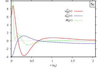
(b)

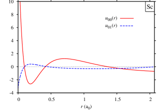
Figure 1: (Color Online) (a) Normalized radial basis response functions $u_{00}^{\mathrm{Sc}(1)}(r)$ [(red) solid line] and $u_{01}^{\mathrm{Sc}(1)}(r)$ [(blue) dashed line] as obtained from Eqs. (28) and (29) for angular momentum $l=0$ calculated in the MT sphere of the Sc atom in rock-salt ScN. The perturbing potential $M_{I}(r)$ is shown as the (green) dotted line. (b) Corresponding radial LAPW basis functions $u_{00}^{\mathrm{Sc}}(r)$ [Eq. (12)] [(red) solid line] and $u_{01}^{\mathrm{Sc}}(r)$ [Eq. (14)] [(blue) dashed line].

The linear change of the matching coefficients $A_{lmp}^{a}(\mathbf{k},\mathbf{G})$ is straightforwardly obtained from differentiating Eq. (10) with respect to the potential. This finally gives rise to

$$A_{lmp,I}^{a(1)}(\mathbf{k},\mathbf{G})\\ =(-1)^{p+1}\frac{[u_{l\overline{p}}^{a}(S^{a}),\sum_{p^{\prime}}A_{lmp^{\prime}}^{a}(\mathbf{k},\mathbf{G})u_{lp^{\prime},I}^{a(1)}(S^{a})]}{[u_{l1}^{a}(S^{a}),u_{l0}^{a}(S^{a})]}\,.$$ (33)

The coefficients $A_{lmp,I}^{a(1)}(\mathbf{k},\mathbf{G})$ guarantee that the resulting functions $\phi_{\mathbf{k}\mathbf{G},I}^{(1)}(\mathbf{r})$, as defined in Eq. (27), and their radial derivatives continuously go to zero at the MT sphere boundaries.

We note that the rest of the derivation applies generally to spherical $(L=0)$ and nonspherical perturbations $(L\neq 0)$. Once the $\phi_{\mathbf{k}\mathbf{G},I}^{(1)}(\mathbf{r})$ are constructed, linear combinations with the wave-function coefficients

$$\tilde{\varphi}_{n\mathbf{k},I}^{(1)}(\mathbf{r}) = \sum_{\mathbf{G}}z_{\mathbf{G}}(n,\mathbf{k})\phi_{\mathbf{k}\mathbf{G},I}^{(1)}(\mathbf{r})$$ (34)

yield the second term of Eq. (24) for variations that scale with $M_{I}(\mathbf{r})$ according to Eq. (19).

The first term of Eq. (24), in the following denoted by $\hat{\varphi}_{n\mathbf{k},I}^{(1)}(\mathbf{r})$, lies completely in the Hilbert space spanned by the LAPW basis set. Accordingly, $\hat{\varphi}_{n\mathbf{k},I}^{(1)}(\mathbf{r})$ can be expanded in terms of the unperturbed KS wave functions

$$\hat{\varphi}_{n\mathbf{k},I}^{(1)}(\mathbf{r})=\sum_{n^{\prime}}\langle\varphi_{n^{\prime}\mathbf{k}}|\hat{\varphi}_{n\mathbf{k},I}^{(1)}\rangle\varphi_{n^{\prime}\mathbf{k}}(\mathbf{r})\,.$$ (35)

The projection coefficient $\langle\varphi_{n^{\prime}\mathbf{k}}|\hat{\varphi}_{n\mathbf{k},I}^{(1)}\rangle$ is obtained by exploiting the fact that $\varphi_{n\mathbf{k},I}^{(1)}(\mathbf{r})=\hat{\varphi}_{n\mathbf{k},I}^{(1)}(\mathbf{r})+\tilde{\varphi}_{n\mathbf{k},I}^{(1)}(\mathbf{r})$ is the solution of Eq. (21). After left multiplication of Eq. (21) with $\varphi_{n^{\prime}\mathbf{k}}^{*}(\mathbf{r})$ ($n^{\prime}\neq n$) and integration over space one yields

$$(\epsilon_{n^{\prime}\mathbf{k}}-\epsilon_{n\mathbf{k}})\langle\varphi_{n^{\prime}\mathbf{k}}|\hat{\varphi}_{n\mathbf{k},I}^{(1)}+\tilde{\varphi}_{n\mathbf{k},I}^{(1)}\rangle+\langle D_{n^{\prime}\mathbf{k}}|\hat{\varphi}_{n\mathbf{k},I}^{(1)}+\tilde{\varphi}_{n\mathbf{k},I}^{(1)}\rangle\\ =\langle\varphi_{n^{\prime}\mathbf{k}}|\epsilon_{n\mathbf{k},I}^{(1)}-M_{I}|\varphi_{n\mathbf{k}}\rangle\,,$$ (36)

where we additionally allow for deviations of the calculated wave functions $\varphi_{n^{\prime}\mathbf{k}}(\mathbf{r})$ from the true eigenfunctions of the operator $H$ by explicitly treating $D_{n^{\prime}\mathbf{k}}(\mathbf{r})=(H-\epsilon_{n^{\prime}\mathbf{k}})\varphi_{n^{\prime}\mathbf{k}}(\mathbf{r})$ as a nonzero quantity. Using $\langle\varphi_{n^{\prime}\mathbf{k}}|\varphi_{n\mathbf{k}}\rangle=0$ and $\langle D_{n^{\prime}\mathbf{k}}|\hat{\varphi}_{n\mathbf{k},I}\rangle=0$ leads to $\langle\varphi_{n^{\prime}\mathbf{k}}|\hat{\varphi}_{n\mathbf{k},I}^{(1)}\rangle$ for $n\neq n^{\prime}$. The expansion coefficient for $n=n^{\prime}$ follows from the normalization condition Eq. (20).

By adding up $\hat{\varphi}_{n\mathbf{k},I}^{(1)}(\mathbf{r})$ and $\tilde{\varphi}_{n\mathbf{k},I}^{(1)}(\mathbf{r})$ we finally end up with the instructive result

$$\@ADDCLASS{ltx_eqn_lefteqn}$\displaystyle\varphi_{n\mathbf{k},I}^{(1)}(\mathbf{r})=$\mbox{}\hfil\\ \sum_{{n^{\prime}\leq N\atop n^{\prime}(\neq n)}}\left[\frac{\langle\varphi_{n^{\prime}\mathbf{k}}|M_{I}|\varphi_{n\mathbf{k}}\rangle}{\epsilon_{n\mathbf{k}}-\epsilon_{n^{\prime}\mathbf{k}}}+\frac{\langle\varphi_{n^{\prime}\mathbf{k}}|H-\epsilon_{n^{\prime}\mathbf{k}}|\tilde{\varphi}_{n\mathbf{k},I}^{(1)}\rangle}{\epsilon_{n\mathbf{k}}-\epsilon_{n^{\prime}\mathbf{k}}}\right]\varphi_{n^{\prime}\mathbf{k}}(\mathbf{r})\\ +\int d^{3}r^{\prime}\left[\delta(\mathbf{r}-\mathbf{r}^{\prime})-\sum_{n^{\prime}\leq N}\varphi_{n^{\prime}\mathbf{k}}(\mathbf{r})\varphi_{n^{\prime}\mathbf{k}}^{*}(\mathbf{r}^{\prime})\right]\tilde{\varphi}_{n\mathbf{k},I}^{(1)}(\mathbf{r}^{\prime})\,.$$ (37)

The first term contains the usual expression from first-order perturbation theory [Eq. (22)] and a correction that takes into account that the wave functions are not exact eigenfunctions of the Hamiltonian operator $H$ due to the incompleteness of the basis. We call this correction the Pulay term in analogy to a corresponding term – the Pulay force – in atomic-force calculations.J. M. Soler and A. R. Williams (1989); R. Yu, D. Singh, and H. Krakauer (1991); foo (b) As already discussed, the first term is inaccurate because of the truncation of the sum $\left(n^{\prime}\leq N\right)$. This inaccuracy is corrected by the second term that arises from the explicit variation of the basis due to a change in the effective potential. We call this term the basis-response (BR) correction. In the limit of a complete basis (with an infinite number of states) the Pulay and BR term would vanish, and the standard perturbation theory (SPT) expression would give the exact result. The sum over states in the BR part can be interpreted as a double-counting correction that subtracts response contributions already contained in the first term.

So far, we have restricted the derivation to the augmented plane waves defined in Eq. (9). Corresponding corrections can be derived for the local orbitals and the core states. While the derivation for the former closely follows the steps already presented, the core states require some different considerations. In contrast to the basis functions, they fulfill the boundary condition that they approach zero for $r\rightarrow\infty$. This boundary condition is used to determine the energies of the core levels, which in contrast to the construction of the LAPW basis functions are not chosen as parameters but result from an atomic eigenvalue problem. Therefore, we use a finite-difference approach: we solve the atomic eigenvalue problems for the perturbed potentials $V_{\mathrm{eff},0}(r)+\frac{\lambda}{2}M_{I}(r)$ and $V_{\mathrm{eff},0}(r)-\frac{\lambda}{2}M_{I}(r)$ with $\lambda=0.0001$, take the difference of the resulting core wave functions, and divide by $\lambda$, which directly yields the linear response of the core state. As the fully relativistic Dirac equation is employed for the core states, the finite-difference approach yields the solution of the fully relativistic Sternheimer equation.

Finally we use Eq. (37) to construct the density response matrix [Eq. (16)] and the right-hand side of the OEP equation [Eq. (17)]; also consider Eqs. (3) and (19). As a result,

$$\chi_{\mathrm{s},IJ}=4\sum_{n\mathbf{k}}^{\mathrm{occ.}}\sum_{n^{\prime}\leq N}^{\mathrm{unocc.}}\left[\frac{\langle M_{I}\varphi_{n\mathbf{k}}|\varphi_{n^{\prime}\mathbf{k}}\rangle\langle\varphi_{n^{\prime}\mathbf{k}}|\varphi_{n\mathbf{k}}M_{J}\rangle}{\epsilon_{n\mathbf{k}}-\epsilon_{n^{\prime}\mathbf{k}}}\right.\\ \left.\hphantom{2\sum_{n\mathbf{k}}^{\mathrm{occ.}}\sum_{n^{\prime}\leq N}^{\mathrm{unocc.}}}+\frac{\langle M_{I}\varphi_{n\mathbf{k}}|\varphi_{n^{\prime}\mathbf{k}}\rangle\langle\varphi_{n^{\prime}\mathbf{k}}|H-\epsilon_{n^{\prime}\mathbf{k}}|\tilde{\varphi}_{n\mathbf{k},J}^{(1)}\rangle}{\epsilon_{n\mathbf{k}}-\epsilon_{n^{\prime}\mathbf{k}}}\right]\\ +4\sum_{n\mathbf{k}}^{\mathrm{occ.}}\left[\langle M_{I}\varphi_{n\mathbf{k}}|\tilde{\varphi}_{n\mathbf{k},J}^{(1)}\rangle\hskip 71.13188pt\vphantom{\sum_{n^{\prime}\leq N}}\right.\\ \left.-\sum_{n^{\prime}\leq N}\langle M_{I}\varphi_{n\mathbf{k}}|\varphi_{n^{\prime}\mathbf{k}}\rangle\langle\varphi_{n^{\prime}\mathbf{k}}|\tilde{\varphi}_{n\mathbf{k},J}^{(1)}\rangle\right]\,,$$ (38)

and

$$t_{I}=4\sum_{n\mathbf{k}}^{\mathrm{occ.}}\sum_{n^{\prime}\leq N}^{\mathrm{unocc.}}\left[\frac{\langle M_{I}\varphi_{n\mathbf{k}}|\varphi_{n^{\prime}\mathbf{k}}\rangle}{\epsilon_{n\mathbf{k}}-\epsilon_{n^{\prime}\mathbf{k}}}\langle\varphi_{n^{\prime}\mathbf{k}}|V_{\mathrm{x}}^{\mathrm{NL}}|\varphi_{n\mathbf{k}}\rangle\right.\\ \left.+\frac{\langle\tilde{\varphi}_{n\mathbf{k},I}^{(1)}|H-\epsilon_{n^{\prime}\mathbf{k}}|\varphi_{n^{\prime}\mathbf{k}}\rangle}{\epsilon_{n\mathbf{k}}-\epsilon_{n^{\prime}\mathbf{k}}}\langle\varphi_{n^{\prime}\mathbf{k}}|V_{\mathrm{x}}^{\mathrm{NL}}|\varphi_{n\mathbf{k}}\rangle\right]\\ +4\sum_{n\mathbf{k}}^{\mathrm{occ.}}\left[\langle\tilde{\varphi}_{n\mathbf{k},I}^{(1)}|V_{\mathrm{x}}^{\mathrm{NL}}|\varphi_{n\mathbf{k}}\rangle\vphantom{\sum_{n^{\prime}\leq N}}\right.\\ \left.\hphantom{+2\sum_{n\mathbf{k}}}-\sum_{n^{\prime}\leq N}\langle\tilde{\varphi}_{n\mathbf{k},I}^{(1)}|\varphi_{n^{\prime}\mathbf{k}}\rangle\langle\varphi_{n^{\prime}\mathbf{k}}|V_{\mathrm{x}}^{\mathrm{NL}}|\varphi_{n\mathbf{k}}\rangle\right]\,.$$ (39)

are again given as a sum over an SPT, Pulay, and BR term.

In its present form, the expression in Eq. (38) breaks the Hermiticity of $\chi_{\mathrm{s},IJ}$ because the additional term is formally asymmetric in the indices $I$ and $J$. However, the numerical deviation from Hermiticity is small. To eliminate these inaccuracies, we take the average $(\chi_{\mathrm{s},IJ}+\chi_{\mathrm{s},JI}^{*})/2$.

V Performance of the IBC

We have implemented the incomplete-basis-set correction (IBC), as described in the previous section, in the Fleur program package,Fle which is based on the FLAPW method. Before showing results for the nitrides BN, AlN, GaN, InN, and ScN as well as the perovskites $\mathrm{CaTiO}_{3}$, $\mathrm{SrTiO}_{3}$, and $\mathrm{BaTiO}_{3}$ in the next section, we first analyze in detail how the convergence properties of the single-particle response function [Eq. (38)], the local exchange potential, and the band gap are improved by the IBC for the example of rock-salt scandium nitride. The improvements are twofold: (1) the spherical response function converges with much smaller LAPW basis sets than before; (2) for a given LAPW basis much fewer unoccupied states are needed for its construction.

Unless noted otherwise, the LAPW cutoff parameters $G_{\mathrm{max}}=3.8\,a_{0}^{-1}$ and $l_{\mathrm{max}}=8$ were used for the calculations of rock-salt $\mathrm{ScN}$ at the experimental lattice constant of $8.50\,a_{0}$ ($a_{0}$ is the Bohr radius). The Sc $1s$, $2s$, and $2p$ states as well as the N $1s$ state are treated as core states. All other states – including the $3s$ and $3p$ semicore states of Sc – are treated as valence. The Brillouin zone is sampled with a 4$\times$4$\times$4 $\mathbf{k}$-point mesh.

V.1 Response function

We remind the reader that the IBC consists of two terms, the Pulay and the BR term, which are derived as a correction for the expression of standard perturbation theory abbreviated by SPT. In principle, the core states are included in Eq. (38) as part of the sum over the occupied states. This is reminiscent of the fact that the IBC not only corrects for the incompleteness of the basis, but also comprises the exact core-state response, which will give a numerically important contribution, but only a nearly rigid shift of the convergence curves. To simplify the discussion, we will leave the contribution of the core states out until later.

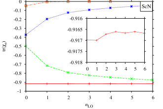
Figure 2: (Color Online) Convergence of the trace of $\chi_{\mathrm{s}}$ for $\mathrm{ScN}$ as a function of the number of local orbitals $n_{\mathrm{LO}}$ per $l$ quantum number $\left(0\leq l\leq 4\right)$ and atom. The SPT [(green) dashed], BR [(blue) dotted], and Pulay term [(orange) dot-dashed] as well as their sum [(red) solid line] are shown, respectively. We only consider spherical MPB functions, and the (constant) contribution of core states is neglected.

Figure 2 shows the convergence of the trace of the matrix $\chi_{\mathrm{s},IJ}$ [Eq. (38)] as well as its SPT, Pulay, and BR contributions for ScN as a function of the number of local orbitals $n_{\mathrm{LO}}$ added to the LAPW basis for each $lm$ channel with $0\leq l\leq 4$ and $|m|\leq l$ (in addition to local orbitals already used for the semicore $3s$ and $3p$ states of scandium). The added local orbitals are placed at energies in the conduction band according to the recipe of Ref. M. Betzinger, C. Friedrich, S. Blügel, and A. Görling, 2011. For simplicity, we have employed the same number of additional local orbitals for Sc and N. In this case the MPB consists of 13 spherical functions, seven at the Sc atom and six at the N atom. The trace $\mathrm{tr}(\chi_{\mathrm{s}})=\sum_{I}\chi_{\mathrm{s},II}$ is restricted to these functions. The slow convergence of the SPT [dashed (green) line] is a direct consequence of the low flexibility of the LAPW basis in the MT spheres with respect to changes of the effective potential. The dotted (blue) and dot-dashed (orange) line show the corresponding behavior of the BR and Pulay-term, respectively. As expected, both corrections become smaller as the basis set becomes more and more complete toward $n_{\mathrm{LO}}=6$. The major part of the correction originates from the BR term, while the Pulay term is significant only for $n_{\mathrm{LO}}=0$ and, even there, accounts for merely 10% of the total IBC. For $n_{\mathrm{LO}}\geq 1$, it rapidly approaches zero. The BR term is much more important numerically. In fact, the dotted (blue) and dashed (green) lines appear to be mirror images of one another, showing that the BR correction compensates nearly exactly for what is missing in the SPT term. The sum of all terms produces the solid (red) line, which appears to be constant on the scale of the diagram. From the inset, which shows the curve on a much finer scale, we see that the variations are below 0.05 %, an accuracy that we could never hope to achieve without the IBC. For this particular case, we thus do not have to employ additional local orbitals (i.e., $n_{\mathrm{LO}}=0$) for the unoccupied states.

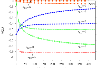
Figure 3: (Color Online) Convergence of the trace of $\chi_{\mathrm{s}}$ for $\mathrm{ScN}$ as a function of the number of unoccupied states $N-N_{\mathrm{el}}/2$ . The SPT [(green) open symbols], BR [(blue) filled symbols], and Pulay term [(orange) hall-filled symbols] as well as their sum [(red) open symbols] are shown, respectively. Circles and squares are used to distinguish the cases $n_{\mathrm{LO}}=0$ and $n_{\mathrm{LO}}=6$.

Up to now, we have discussed how the IBC affects the convergence of the single-particle response function with respect to the quality of the LAPW basis. A perhaps more obvious convergence parameter is the number of states $N$ included in the evaluation of Eq. (38). All three terms, SPT, Pulay, and BR, involve summations over the unoccupied states up to the maximal band index $N$. Keeping in mind that the sum in the BR part can be interpreted as a double-counting correction, one can hope that the function $\tilde{\varphi}_{n\mathbf{k},I}^{(1)}(\mathbf{r})$ obtained nonperturbatively from direct integration of the Sternheimer equation already contains, to a certain degree, information about the whole infinite spectrum of unoccupied states. As a matter of fact, this conjecture is substantiated by Fig. 3, which shows the convergence of the trace of $\chi_{\mathrm{s}}$ for two different LAPW basis sets with $n_{\mathrm{LO}}=0$ (circles) and $n_{\mathrm{LO}}=6$ (squares) as a function of the number of unoccupied states $N-N_{\mathrm{el}}/2$, where $N_{\mathrm{el}}$ is the number of valence electrons per unit cell ($N_{\mathrm{el}}=16$ for ScN). (The reciprocal cutoff value of the LAPW basis has been increased to $G_{\mathrm{max}}=5.5\,a_{0}^{-1}$ to generate up to 450 bands.) Similarly to Fig. 2, the SPT term [(green) open symbols] shows a very slow convergence with respect to the number of unoccupied states. We note that in the $n_{\mathrm{LO}}=0$ case [(green) open circles] a large part of the response is actually missing in the SPT term resulting in a false convergence behavior of the curve, which seems to converge, but toward a wrong value. As above, the BR term [(blue) filled symbols] is much more important than the Pulay term [(orange) half-filled circles] and counterbalances the first term almost exactly. While the Pulay term is practically zero in the case $n_{\mathrm{LO}}=6$, also compare Fig. 2, it is significant in the case $n_{\mathrm{LO}}=0$ and yields a small but important contribution to the sum of all terms. In fact, this sum nearly follows the same curve [(red) open symbols, circles and squares correspond to $n_{\mathrm{LO}}=0$ and $n_{\mathrm{LO}}=6$, respectively] in the two cases, showing again that with the IBC we can restrict ourselves to the conventional LAPW basis, i.e., $n_{\mathrm{LO}}=0$. The total sum converges extremely fast, thanks to the BR term, in which the infinite spectrum of eigenstates is already incorporated to a large extent. Without showing further results we note that the IBC affects the convergence of the right hand side [Eq. (39)] in a similarly beneficial way.

So far, we have not discussed the contribution of the core states to the density response $\chi_{\mathrm{s}}$. For the core state response we solve a fully relativistic Sternheimer equation by a finite-difference approach as discussed in Sec. IV.1. The resulting solution embodies the full infinite spectrum of unoccupied states by construction and can, therefore, be considered to represent already the exact core-state response (up to numerical errors connected with the finite-difference approach, which can be made arbitrarily small, though). Therefore, we can set $N$ to the number of occupied states in Eq. (38). The first term is then zero, and only the BR term remains.

The contribution of the core states to the response function is numerically important. In the case of ScN it is more than four times larger than the valence contribution. However, it should be noted that the effective quantity for the construction of the local exchange potential is not the response function itself, but its inverse [see Eq. (4)]. Therefore, large eigenvalues of $\chi_{\mathrm{s}}$ become comparatively unimportant in $\chi_{\mathrm{s}}^{-1}$. This is confirmed by the following observation. We find that the SPT expression alone is incapable of describing the core-state response. Even with $n_{\mathrm{LO}}=6$ and $N=450$, only about $20\%$ of the contribution of the core states is accounted for, which manifests the hardly surprising fact that the LAPW valence basis is unsuitable to describe changes in the core states. However, this shortcoming affects the resulting exchange potential and KS transition energies only slightly, as we will see below.

V.2 Local exchange potential

Figure 4 shows the local exact exchange potential between neighboring scandium and nitrogen atoms for three calculations, all of them without any local orbitals for the unoccupied states. For these calculations an MPB with $G_{\mathrm{max}}^{\prime}=2.8\,a_{0}^{-1}$ and $L_{\mathrm{max}}=4$ is employed, and the IBC is applied to both core and valence electrons. Without the IBC (green dashed line) we obtain an unphysical, strongly varying potential that even tends to an unreasonable positive value at the position of the nitrogen nucleus. In Ref. M. Betzinger, C. Friedrich, S. Blügel, and A. Görling, 2011 we showed that the spurious oscillations can be avoided by augmenting the LAPW basis with local orbitals leading to a smooth and physical potential, at the expense of a very costly calculation. As shown in Fig. 4, the same smooth shape of the local exact exchange potential is realized by employing the IBC with a considerably smaller computational overhead. We emphasize that no local orbitals are used in this calculation.

When one watches closely, one still sees very slight anomalies of the dotted curve at the atomic nuclei, here more pronounced at the nitrogen nucleus (also cf. the insets). These result from the fact that the radial MT potential enters with a factor $r^{2}$ into the equations. The region close to the nuclei has only little weight and is therefore difficult to converge. On the one hand, for small $r$ the total effective potential is dominated by the potential of the nucleus $-Z/r$ as well as the centrifugal kinetic energy barrier $l(l+1)/(2r^{2})$ such that slight inaccuracies at the nuclei prove to be irrelevant in the calculation of the electronic structure. On the other hand, we can find a simple remedy by an additional constraint for the spherical functions $(L=0)$ of the MPB, which has the additional benefit of reducing their number by one for each atom in the unit cell. We require the gradient of these functions to vanish at $r=0$. As already mentioned in Sec. III, this behavior has been observed for the local exact exchange potential in previous publications.J. B. Krieger, Y. Li, and G. J. Iafrate (1992); D. Ködderitzsch, H. Ebert, and E. Engel (2008); D. Ködderitzsch, H. Ebert, H. Akai, and E. Engel (2009) Thus, the constraint does not induce errors. With such a modified MPB the anomalies of $V_{\mathrm{x}}(\mathbf{r})$ at the nuclei disappear, and we obtain the red solid line shown in Fig. 4. We also note that the numerical stability benefits from this modification.

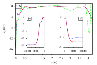
Figure 4: (Color Online) Local EXX potential for ScN on a line connecting the neighboring Sc and N atoms. We have used a conventional LAPW basis without local orbitals for the unoccupied states. The (blue) dotted and (green) dashed curves correspond to calculations with and without the IBC. For the (red) solid curve we have employed an additional constraint for the MPB (see text). Eq. (4) defines the potential only up to a constant. Here, we use the convention $\int V_{\mathrm{x}}(\mathbf{r})\,d^{3}r=0$.

As already pointed out, the IBC is presently only applied to spherical variations of the potential. To converge the nonspherical contributions properly we still need a few local orbitals. Figure 5(a) shows this effect, which is strongest close to the atomic nucleus of Sc. Using a single set of local orbitals, i.e., $n_{\mathrm{LO}}=1$, gives a slight correction of the potential, which gives rise to changes in single-particle transition energies in the order of $0.10-0.15\,\mathrm{eV}$. (We have considered the gap transitions $\Gamma\rightarrow\Gamma$, $\Gamma\rightarrow\mathrm{X}$, and $\Gamma\rightarrow\mathrm{L}$.) For $n_{\mathrm{LO}}=2$ changes are less than $0.03\,\mathrm{eV}$. It is important to note that the calculations always converge to the same result, irrespective of whether or not the IBC is used. We expect that once the IBC is extended to the nonspherical MPB functions, no extra local orbitals are required anymore.

As already discussed, taking into account the exact core response yields a numerically important contribution to the single-particle response function. To demonstrate the effect on the local exchange potential, we switch the IBC for the core states off. Figure 5(b) shows that this has only a comparatively small effect on the shape of the resulting potential. At first sight, the incurred changes in the potential are more pronounced than in Fig. 5(a), but, in contrast to Fig. 5(a), they mostly affect the region close to the nucleus, where the effective potential is dominated by the potential of the nucleus and the angular kinetic energy. In fact, the single-particle transition energies are influenced only little: they change by less than 0.04 eV. However, it should be noted that the exact core response is evaluated at virtually no extra cost.

(a)(b)

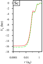
Figure 5: (Color Online) (a) Comparison of $V_{\mathrm{x}}(\mathbf{r})$ close to the atomic nucleus of Sc for calculations with [(green) dashed line, $n_{\mathrm{LO}}=1$] and without [(red) solid line, $n_{\mathrm{LO}}=0$] local orbitals. (b) $V_{\mathrm{x}}(\mathbf{r})$ with [(red) solid line] and without [(green) dashed line] the core response of the IBC.

V.3 KS band gap

After discussing the effect of the IBC on the ingredients of the OEP integral equation and the local exact exchange potential, we now turn to the KS band gap. As we have presently derived the IBC only for the spherical MPB functions, we employ the cutoff $L_{\mathrm{max}}=0$ for this test calculation in order to highlight the improvements resulting from the IBC. This will produce a potential $V_{\mathrm{x}}(r)$ that is purely spherical in the muffin-tin spheres. We note again that a generalization to nonspherical functions $(L>0)$ is possible, but not yet implemented. Furthermore, we restrict the interstitial exchange potential to a constant for simplicity.

Figure 6 shows the direct $(\Gamma\rightarrow\Gamma)$ gap of ScN for this specific numerical setup as a function of the number of local orbitals per $l$ channel added to the LAPW basis. The case $n_{\mathrm{LO}}=6$ corresponds to $300$ additional basis functions. It is known that small inaccuracies in the band gap can occur due to the linearization error of the LAPW basis (in the case $n_{\mathrm{LO}}=0$). To eliminate this pure basis-set effect, we have taken two measures: (1) we have performed only a single EXX-OEP iteration (starting from a PBEJ. P. Perdew, K. Burke, and M. Ernzerhof (1996) ground state), and (2) the final diagonalization of the KS Hamiltonian was performed with the most accurate basis set $(n_{\mathrm{LO}}=6)$. The value $n_{\mathrm{LO}}$ shown on the abscissa thus corresponds to the basis used in solving the OEP equation, and variations in the band gap can be attributed exclusively to the precision of the local exchange potential without additional basis-set effects. We note that, in spite of the very small MPB used here and in spite of performing only one iteration, the resulting band gap is surprisingly close to the fully converged one (see Tab. 1).

Without the IBC [(green) dashed curve] four sets of local orbitals $(n_{\mathrm{LO}}=4)$ are necessary to obtain a direct gap with an accuracy of $0.05\,\mathrm{eV}$ (we note that, judging from the form of the curve, the accuracy at $n_{\mathrm{LO}}=3$ seems to be due to a fortuitous cancellation of errors). On the other hand, the calculation with the IBC yields a reliable gap with an accuracy of $0.007\,\mathrm{eV}$ already without any local orbitals for the unoccupied states $(n_{\mathrm{LO}}=0)$. Both curves converge to the same band-gap value, while the convergence of the IBC values is hardly visible on the scale of the diagram. We have indicated the computation time on the right scale. The computational overhead of the IBC calculations is due to the additional evaluation of the Pulay and BR term, in particular for the matrix elements $\langle\varphi_{n\mathbf{k}}|V_{x}^{\mathrm{NL}}|\tilde{\varphi}_{n\mathbf{k},I}\rangle$ in Eq. (39). It is difficult to compare the efficiency of the calculations, since the least accurate calculation with the IBC is still more accurate than the most accurate one without. If we take an accuracy of $0.05\,\mathrm{eV}$ as a criterion, one would deduce an acceleration of the code by a factor of four. Using less unoccupied states (cf. Fig. 3) could further reduce the computation time.

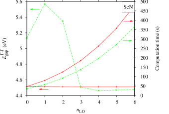
Figure 6: (Color Online) Convergence of the direct gap of ScN with respect to the number of local orbitals $(n_{\mathrm{LO}})$ added to the LAPW basis for one-shot EXX calculations with [(red) solid line] and without [(green) dashed line)] the IBC. The computation time is shown on the right scale.

VI Results and Discussion

In Table 1 we report KS transition energies, i.e., KS eigenvalue differences, for the III-V nitrides in the zincblende structure and for rock-salt ScN, calculated with the EXX and EXXc functionals. The latter contains additionally the LDA correlation functional in the parametrization of Perdew and Zunger.J. P. Perdew and A. Zunger (1981) While the ground-state crystal structure of the III-V nitrides is wurtzite, they can be synthesized in the metastable zincblende structure by epitaxial growth techniques. All calculations were performed at the experimental lattice constants (ScN, $8.50\,a_{0}$; BN, $6.84\,a_{0}$; AlN, $8.26\,a_{0}$; GaN $8.50\,a_{0}$; InN $9.41\,a_{0}$) with an 8$\times$8$\times$8 $\mathbf{k}$-point sampling and with local orbitals for the complete semicore shell (e.g., $2s$ and $2p$ states of Al). The numerical cutoff parameters $G_{\mathrm{max}}$, $G^{\prime}_{\mathrm{max}}$, $l_{\mathrm{max}}$, and $L_{\mathrm{max}}$ as well as the number of local orbitals are determined such that the transition energies are converged to within $10\,\mathrm{meV}$. We compare our results with plane-wave pseudopotential calculations and experimental values from the literature.

The EXX and EXXc functionals give KS transition energies that are much closer to the experimental value than LDA. InN and ScN, which are metallic in LDA, are correctly predicted to be semiconductors. The inclusion of the LDA correlation functional in EXXc increases the values by about $0.01-0.2\,\mathrm{eV}$, but does not yield a systematic improvement when compared to experiment. For AlN and ScN our EXXc values agree well with those from the pseudopotential studies. The differences are mostly of the same order as the differences in the LDA transition energies.

In the case of GaN and InN the situation is more complex because of the semicore $d$ states. In pseudopotential calculations they can be treated approximately as atomic core states in the pseudopotential or, at a considerably larger computational expense, as valence electrons within the plane-wave basis. Therefore, Table 1 lists two values for each system and functional from calculations where the $d$ semicore electrons are treated as valence ("with $d$") or not ("no $d$"). The former values, which are systematically smaller than the latter, must be considered to be more accurate. Of course, we do not have to make such a distinction in our calculations, because the FLAPW method treats valence and core electrons, down to the $1s$ state, on an equal footing. Indeed, our LDA transition energies compare better with the pseudopotential calculations "with $d$". However, we find a much larger discrepancy for the EXXc functional. In all cases the all-electron values fall in-between the two pseudopotential results, often being equally far away from either value. Engel and SchmidE. Engel and R. N. Schmid (2009) pointed out for the case of transition metal monoxides that the complete semicore shell, comprising the $3s$, $3p$, and $3d$ states, must be treated as valence to obtain accurate EXX values within the pseudopotential approach. It is to be expected that this also holds for GaN and InN, which would explain the discrepancies observed for the pseudopotential calculations with respect to the all-electron results.

Table 1: KS transition energies (in eV) obtained with the LDA, EXX, and EXXc potentials for the III-V nitrides and $\mathrm{ScN}$. An $8\times 8\times 8$ $\mathbf{k}$-point sampling has been employed for all calculations. For comparison, plane-wave pseudopotential results and experimental values from the literature are given.

		This work			Plane-wave PP
		LDA	EXX	EXXc	LDA		EXXc		Expt.
$\mathrm{ScN}$	$\Gamma\rightarrow\Gamma$	$2.35$	$4.41$	$4.42$	$\hphantom{-}2.34^{c}$		$4.59^{c}$, $4.7^{d}\hphantom{0}$		$3.8^{d}$
	$\Gamma\rightarrow\mathrm{X}$	$-0.14$	$1.58$	$1.67$	$-0.15^{c}$		$1.7^{c}\hphantom{0}$,$1.6^{d}\hphantom{0}$		$1.3^{d}$
	$\mathrm{X}\rightarrow\mathrm{X}$	$0.79$	$2.48$	$2.56$	$\hphantom{-}0.75^{c}$		$2.59^{c}$,$2.9^{d}\hphantom{0}$		$2.40^{d}$
$\mathrm{BN}$	$\Gamma\rightarrow\Gamma$	$8.68$	$9.80$	$9.88$
	$\Gamma\rightarrow\mathrm{L}$	$10.18$	$10.88$	$10.95$
	$\Gamma\rightarrow\mathrm{X}$	$4.34$	$5.42$	$5.58$					$6.4^{e}$
$\mathrm{AlN}$	$\Gamma\rightarrow\Gamma$	$4.20$	$5.46$	$5.59$	$\hphantom{-}4.27^{b}$		$5.66^{a}$,$5.74^{b}$		$5.93^{f}$
	$\Gamma\rightarrow\mathrm{L}$	$7.24$	$8.42$	$8.55$	$\hphantom{-}7.25^{b}$		$8.58^{b}$
	$\Gamma\rightarrow\mathrm{X}$	$3.22$	$4.77$	$4.96$	$\hphantom{-}3.27^{b}$		$5.03^{a}$,$5.06^{b}$		$5.3^{f}$
					no $d$	with $d$	no $d$	with $d$
$\mathrm{GaN}$	$\Gamma\rightarrow\Gamma$	$1.76$	$3.11$	$3.24$	$2.22^{b}$	$\hphantom{-}1.65^{b}$	$3.52^{b}$	$2.88^{b}$	$3.27^{g}$
	$\Gamma\rightarrow\mathrm{L}$	$4.55$	$5.94$	$6.05$	$4.88^{b}$	$\hphantom{-}4.43^{b}$	$6.23^{b}$	$5.64^{b}$
	$\Gamma\rightarrow\mathrm{X}$	$3.25$	$4.61$	$4.80$	$3.43^{b}$	$\hphantom{-}3.30^{b}$	$4.99^{b}$	$4.66^{b}$
$\mathrm{InN}$	$\Gamma\rightarrow\Gamma$	$-0.41$	$0.98$	$1.12$	$0.27^{b}$	$-0.44^{b}$	$1.49^{b}$	$0.81^{b}$	$0.596^{h}$,$0.61^{g}$
	$\Gamma\rightarrow\mathrm{L}$	$3.01$	$4.37$	$4.50$	$3.51^{b}$	$\hphantom{-}2.95^{b}$	$4.75^{b}$	$4.14^{b}$
	$\Gamma\rightarrow\mathrm{X}$	$2.83$	$4.23$	$4.42$	$2.87^{b}$	$\hphantom{-}2.82^{b}$	$4.63^{b}$	$4.20^{b}$

aReference	M. Städele, M. Moukara, J. A. Majewski, P. Vogl, and A. Görling,1999
bReference	A. Qteish, A. I. Al-Sharif, M. Fuchs, M. Scheffler, S. Boeck, and J. Neugebauer,2005
cReference	A. Qteish, P. Rinke, M. Scheffler, and J. Neugebauer,2006
dReference	D. Gall, M. Städele, K. Järrendahl, I. Petrov, P. Desjardins, R. T. Haasch, T. Y. Lee, and J. E. Greene,2001
eReference	R. M. Chrenko,1974
fReference	M. Röppischer, R. Goldhahn, G. Rossbach, P. Schley, C. Cobet, N. Esser, T. Schupp, K. Lischka, and D. J. As,2009
gReference	H. Okumura, K. Ohta, K. Ando, W. W. Rühle, T. Nagatomo, and S. Yoshida,1997
hReference	P. Schley, C. Napierala, R. Goldhahn, G. Gobsch, J. Schörmann, D. J. As, K. Lischka, M. Feneberg, K. Thonke, F. Fuchs, and F. Bechstedt,2008
gReference	J. Schörmann, D. J. As, K. Lischka, P. Schley, R. Goldhahn, S. F. Li, W. Löffler, M. Hetterich, and H. Kalt,2006

Table 2 shows the energetic positions of the $d$ levels in GaN and InN with respect to the Fermi level, which is fixed at the valence band edge. It is well known that the LDA underbinds the $3d$ states, which is usually attributed to the self-interaction error of LDA. However, in spite of the fact that the EXX(c) is free of this error, the position of the $d$ bands is hardly improved. While in GaAs the $d$ levels are lowered by about $1\,\mathrm{eV}$, they remain nearly at the same energy in InN. In comparison to the experimental values, $17.7\,\mathrm{eV}$ (GaN) and $14.9\,\mathrm{eV}$ (InN; measured for wurtzite structure), this is hardly an improvement over LDA. On the other hand, we find that the HF method yields $d$-band positions at $21.28\,\mathrm{eV}$ (GaN) and $18.22\,\mathrm{eV}$ (InN), respectively, i.e., even below the experiment. As the HF and EXX-OEP methods employ the same energy functional, the question arises why the $d$-band positions appear at different energies. In short, what is the meaning of the EXX-OEP single-particle energies? According to Koopmans’ theorem,T. Koopmans (1934) the single-particle energies in the HF approach can be understood as total-energy differences between an excited state and the ground state, neglecting orbital relaxation effects. For the $d$ states, $\Delta E=E_{d}^{N-1}-E_{0}^{N}=\langle d|h^{\mathrm{HF}}|d\rangle=\epsilon_{d}^{\mathrm{HF}}$, where the two total energies correspond to the many-body states with and without a hole in a $d$ level, $\epsilon_{d}^{\mathrm{HF}}$ is the HF single-particle energy of that $d$ level, and $h^{\mathrm{HF}}$ is the HF single-particle Hamiltonian. The OEP approach was originally intended as a procedure to simplify the solution of the HF equations by introducing a local potential that minimizes the HF total energy. In fact, the EXX-OEP and HF ground-state total energies are nearly identical.M. Betzinger, C. Friedrich, S. Blügel, and A. Görling (2011); A. Hesselmann, A. W. Götz, F. D. Sala, and A. Görling (2007) This indicates that the slight difference in shape of the single-particle wave functions only has a negligible effect on the ground-state total energy $E_{0}^{N}$, a statement that should also hold for the hole-state energy $E_{d}^{N-1}$. Using Koopman’s theorem again with the EXX-OEP wave functions instead of the HF ones, we should obtain practically the same $\Delta E$. However, as seen in Table 2, the HF eigenvalue $\epsilon_{d}^{\mathrm{HF}}$ differs from the corresponding EXX-OEP eigenvalue $\epsilon_{d}^{\mathrm{EXX}}$ by $\Delta=\epsilon_{d}^{\mathrm{HF}}-\epsilon_{d}^{\mathrm{EXX}}=\langle d|V_{\mathrm{x}}^{\mathrm{NL}}-V_{\mathrm{x}}|d\rangle$. As a consequence, the underbinding of the $d$ bands in LDA – and also in EXX(c) – cannot be solely ascribed to the self-interaction error contrary to common belief. Part of this underbinding is due to the forced locality of the effective potential, which gives rise to a nonzero energy shift that is very similar in spirit to the derivative discontinuityJ. P. Perdew and M. Levy (1983); L. J. Sham and M. Schlüter (1983) of the xc functional. Even with the exact functional we cannot expect that the $d$-band positions lie at the experimental positions in the same way as we cannot expect the KS band gap to equal the experimental gap.

Table 2: Energetic positions of the $d$ levels in GaN and InN in eV with respect to the Fermi energy and averaged over the Brillouin zone and the $d$ bands.

	LDA	EXX	EXXc	HF	Expt.
$\mathrm{GaN}$	$-13.08$	$-13.93$	$-14.15$	$-21.28$	$-17.7^{a}$
$\mathrm{InN}$	$-12.72$	$-12.65$	$-12.83$	$-18.22$	$-14.9^{b}$

aReference	S. A. Ding, G. Neuhold, J. H. Weaver, P. Häberle, K. Horn, O. Brandt, H. Yang, and K. Ploog,1996
bReference	Q. X. Guo, M. Nishio, H. Ogawa, A. Wakahara, and A. Yoshida, 1998 (Measured for the wurtzite compound.)

Finally, we report results for the electronic structure of the perovskite transition-metal oxides $\mathrm{CaTiO_{3}}$, $\mathrm{SrTiO_{3}}$ and $\mathrm{BaTiO_{3}}$. We have calculated the materials in the ideal cubic structure at experimental lattice constants ($\mathrm{CaTiO}_{3},\,7.35\,a_{\mathrm{0}}$; $\mathrm{SrTiO}_{3},\,7.46\,a_{\mathrm{0}}$; $\mathrm{BaTiO_{3},\,7.60\,a_{\mathrm{0}}}$) and with the functionals LDA, EXX, and EXXc. The Ti $3s$ and $3p$ states as well as the first subshell of the cations (Ca, $3s$ $3p$; Sr, $4s$ $4p$; Ba $5s$ $5p$) have been treated with local orbitals. The electronic structures of the three systems are very similar. They are semiconductors with an indirect band gap between the $\mathrm{R}$ and the $\Gamma$ point and a direct gap at the $\Gamma$ point. We compare the LDA and EXX band structures and densities of states of $\mathrm{CaTiO_{3}}$ in Fig. 7. The EXX functional shifts the Ti $3d$ conduction bands away from the O $2p$ valence bands and thus opens the band gap, while the band dispersions remain nearly unaffected. The valence band width is slightly decreased, though.

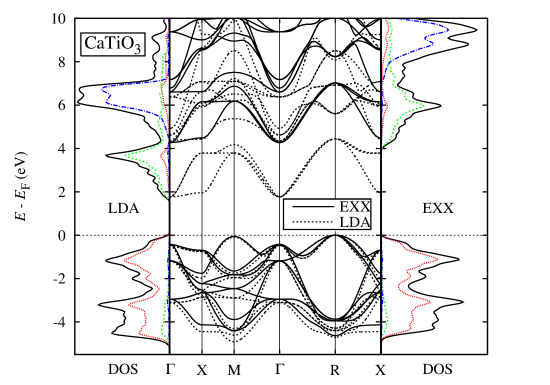
Figure 7: (Color Online) Comparison of the LDA and EXX band structures and densities of states (DOS) for $\mathrm{CaTiO_{3}}$. The total and partial DOS for Ca $3d$, Ti $3d$, and O $2p$ are shown as (black) solid, (blue) dot-dashed, (green) dashed, and (red) dotted lines, respectively.

KS transition energies are reported in Table 3. The LDA underestimates the energies by roughly $50\%$. Although the EXX(c) functionals yield values that are closer to experiment, we observe a pronounced overestimation by about $25\%$. This might be due to two reasons: (1) The fortuitous error cancellation arising from the neglect of correlation on the one hand and of the derivative discontinuity on the other hand does not work for these transition-metal oxides. (2) The ideal cubic structure used in our study does not correspond to the experimentally measured systems. It is known that these perovskite materials undergo a number of structural phase transitions. For example, $\mathrm{SrTiO_{3}}$ is cubic at room temperature but tetragonal at low temperatures. $\mathrm{BaTiO_{3}}$, on the contrary, is cubic at elevated temperatures and tetragonal at room temperature.

Table 3: Direct and indirect KS band gaps (in eV) for cubic $\mathrm{CaTiO}_{3}$, $\mathrm{SrTiO}_{3}$, and $\mathrm{BaTiO}_{3}$ compared with experimental values. A 6$\times$6$\times$6 $\mathbf{k}$-point sampling was employed.

		LDA	EXX	EXXc	Expt.
$\mathrm{CaTiO}_{3}$	$\Gamma\rightarrow\Gamma$	$2.24$	$4.70$	$4.74$
	$\mathrm{R}\rightarrow\Gamma$	$1.77$	$4.28$	$4.31$	$3.57^{a}$
$\mathrm{SrTiO}_{3}$	$\Gamma\rightarrow\Gamma$	$2.09$	$4.51$	$4.54$	$3.75^{b}$
	$\mathrm{R}\rightarrow\Gamma$	$1.73$	$4.20$	$4.22$	$3.25^{b}$
$\mathrm{BaTiO}_{3}$	$\Gamma\rightarrow\Gamma$	$1.81$	$4.08$	$4.12$
	$\mathrm{R}\rightarrow\Gamma$	$1.7$	$4.08$	$4.11$	$3.2^{c}$

aReference	K. Ueda, H. Yanagi, R. Noshiro, H. Hosono, and H. Kawazoe,1998
bReference	K. van Benthem, C. Elsässer, and R. H. French,2001
cReference	S. H. Wemple,1970

VII Conclusions

We have described an efficient way to calculate precise all-electron response functions within the FLAPW method. The key is the development of an incomplete-basis-set correction (IBC), which was derived by describing the response of the LAPW basis functions to changes of the effective potential explicitly by means of radial Sternheimer equations. In this way, the IBC incorporates important response contributions that lie outside the Hilbert space formed by the LAPW basis set. The resulting formula for the response function consists of three terms: the conventional sum-over-states expression of standard perturbation theory (SPT term) and two additional terms, the basis-response and the Pulay term, whose mathematical expression resembles that of the Pulay force of atomic-force calculations. The basis-response term is more important numerically than the Pulay term. Both vanish in the limit of a complete, infinite basis. Together they constitute the IBC, which also yields an explicit and, in principle, exact treatment of the response of the core states that avoids the sum-over-states expression. The total correction is not small. It can be as large as the SPT term.

As a practical example, we have employed the IBC to the EXX-OEP method, an approach that allows the construction of a local exchange potential from the orbital-dependent EXX functional. It involves two response quantities: the density response function and a response function for the single-particle states. We have implemented the IBC for both and demonstrated explicitly for the case of rock-salt scandium nitride that it improves the convergence with respect to the LAPW basis and the number of unoccupied states considerably. While without the correction the solution of the OEP equation requires a highly converged LAPW basis with a large number of local orbitals,M. Betzinger, C. Friedrich, S. Blügel, and A. Görling (2011) no extra local orbitals are needed when we use the IBC. A similar statement can be made about the number of unoccupied states in the sum-over-states expression related to perturbation theory. As the numerical solution of the Sternheimer equation already incorporates the infinite single-particle spectrum to a certain degree, the response function converges at much fewer bands.

With this new scheme we have performed all-electron EXX(c)-OEP calculations for the III-V nitrides in the zincblende structure as well as rock-salt ScN. Our results agree favorably with plane-wave pseudopotential EXXc calculations from the literature. However, larger deviations are observed for GaN and InN, which we attributed to the neglect of semicore states ($3s$, $3p$ of Ga and $4s$, $4p$ of In) in the pseudopotential calculations. This is in accordance with a recent publication by Engel and Schmid.E. Engel and R. N. Schmid (2009) Despite the fact that the EXX functional is self-interaction-free, it does not necessarily improve the position of the $d$ states with respect to LDA, as shown for the semicore $d$ states of GaN and InN. We have explained this observation by the forced locality of the exchange potential, which has the effect that the KS eigenvalues of the occupied states cannot be associated with ionization energies via Koopmans theorem. In order to invoke the latter, extra terms similiar in spirit to the derivative discontinuity of the xc potential have to be considered. Consequently, even with the exact xc potential the $d$ states cannot be expected to appear at the experimental positions.

Furthermore, we discussed the EXX(c) electronic structure of the three cubic perovskites $\mathrm{CaTiO}_{3}$, $\mathrm{SrTiO}_{3}$, and $\mathrm{BaTiO}_{3}$ in comparison with LDA. The EXX functional opens the band gap in all materials but leaves the dispersion of the bands nearly unaffected, except most notably for a slight reduction of the valence band width. While LDA underestimates the band gaps by about $50\%$, the EXX(c) potential overcompensates this error and leads to an overestimation of $25\%$, which we attribute to an incomplete error cancellation between the neglect of correlation and the neglect of the xc derivative discontinuity. On the other hand, differences in the crystal structure between the theoretical setups and experimental realizations might also play a role.

We note that the IBC is a general approach, which is not restricted to the FLAPW method. It applies to all electronic structure methods with a basis set optimized for the effective potential, including those which are atom-centered and based on pre-calculated and tabulated basis sets. Typical electronic structure methods of this type include LMTO,Andersen (1975); H. L. Skriver (1984); Methfessel et al. (2000) DMOL,B. Delley (1990) FHIAIMS,V. Blum, R. Gehrke, F. Hanke, P. Havu, V. Havu, X. Ren, K. Reuter, and M. Scheffler (2009) OPENMX,T. Ozaki (2006) and the SIESTA code.J. M. Soler, E. Artacho, J. D. Gale, A. Garcia, J. Junquera, P. Ordejon, and D. Sanchez-Portal (2002)

Furthermore, with suitable generalizations the IBC can be applied to a broad spectrum of response functions in solid-state physics, e.g., response quantities arising from the displacement of external potentials (e.g. phonons, elastic constants, stress tensor) or from external fields (e.g. g-tensor, chemical shift and nuclear magnetic resonance, dielectric response, infrared and Raman intensities, magneto-elastic and magneto-electric tensors), or from more general perturbations of the Hamiltonian (e.g. Born effective charges, polarizability), to name a few.

Another method that may profit from the IBC is the GW approximation for the electronic self-energy, which involves the calculation of a dynamical density response function and the single-particle Green function. It is well known, and Zinc oxide is a prominent example of it,B.-C. Shih, Y. Xue, P. Zhang, M. L. Cohen, and S. G. Louie (2010); C. Friedrich, M. C. Müller, and S. Blügel (2011) that similarly to the KS response function in EXX-OEP, GW calculations usually converge badly with respect to the basis set and the number of unoccupied states.

Appendix A Scalar-relativistic equations

In the scalar-relativistic approximationD. D. Koelling and B. N. Harmon (1977) for the Dirac equation the large and small radial component, $r^{-1}p(r)$ and $(cr)^{-1}q(r)$, of an electron in a spherical potential $V_{\mathrm{eff},0}(r)$ at energy $\epsilon$ obey the equations of motion

$$\frac{dp(r)}{dr} = 2m_{\mathrm{rel}}q(r)+\frac{1}{r}p(r)$$ (40)

$$\frac{dq(r)}{dr} = -\frac{1}{r}q(r)+wp(r)$$ (41)

with $m_{\mathrm{rel}}=1+[\epsilon-V_{\mathrm{eff,}0}(r)]/(2c^{2})$ ($c$ denotes the speed of light) and $w=[l(l+1)]/[2m_{\mathrm{rel}}r^{2}]+V_{\mathrm{eff},0}(r)-\epsilon$. For a given spherical perturbation that scales with $M(r)$ (index $I$ omitted to simplify the notation), the linear changes of $p(r)$ and $q(r)$ are given by the solutions of the differential equations

$$\frac{dp^{\prime}(r)}{dr} = 2m_{\mathrm{rel}}q^{\prime}(r)+\frac{1}{r}p^{\prime}(r)$$

$$+\frac{1}{c^{2}}[\epsilon^{\prime}-M(r)]q(r)$$

$$\frac{dq^{\prime}(r)}{dr} = -\frac{1}{r}q^{\prime}(r)+wp^{\prime}(r)$$

$$-[1+\frac{l(l+1)}{4m_{\mathrm{rel}}^{2}r^{2}c^{2}}][\epsilon^{\prime}-M(r)]p(r)\,.$$

By direct differentiation we find the differential equations for the energy derivatives $\dot{p}(r)=dp(r)/d\epsilon$ and $\dot{q}(r)=dq(r)/d\epsilon$

$$\frac{d\dot{p}(r)}{dr} = 2m_{\mathrm{rel}}\dot{q}(r)+\frac{1}{r}\dot{p}(r)+\frac{1}{c^{2}}q(r)$$ (44)

$$\frac{d\dot{q}(r)}{dr} = -\frac{1}{r}\dot{q}(r)+w\dot{p}(r)$$

$$-[1+\frac{l(l+1)}{4m_{\mathrm{rel}}^{2}r^{2}c^{2}}]p(r)$$

as well as for the linear changes of $\dot{p}(r)$ and $\dot{q}(r)$

$$\frac{d\dot{p}^{\prime}(r)}{dr} = 2m_{\mathrm{rel}}\dot{q}^{\prime}(r)+\frac{1}{r}\dot{p}^{\prime}(r)$$

$$+\frac{1}{c^{2}}\{[\epsilon^{\prime}-M(r)]\dot{q}(r)+q^{\prime}(r)\}$$

$$\frac{d\dot{q}^{\prime}(r)}{dr} = -\frac{1}{r}\dot{q}^{\prime}(r)+w\dot{p}^{\prime}(r)$$

$$-[1+\frac{l(l+1)}{4m_{\mathrm{rel}}^{2}r^{2}c^{2}}]$$

$$\times\{[\epsilon^{\prime}-M(r)]\dot{p}(r)+p^{\prime}(r)\}$$

$$+\frac{2l(l+1)}{8m_{\mathrm{rel}}^{3}r^{2}c^{4}}[\epsilon^{\prime}-M(r)]p(r)\,.$$

In the nonrelativistic limit $(c\rightarrow\infty)$, these formulas reduce to Eqs. (12), (14), (28), and (29).

References

- Hohenberg and Kohn (1964) P. Hohenberg and W. Kohn, Phys. Rev. 136, B864 (1964).
- C. Fiolhais, F. Noguiera, and M. A. L. Marques (2003) C. Fiolhais, F. Noguiera, and M. A. L. Marques, ed., A Primer in Density Functional Theory, vol. 620 of Lecture Notes in Physics (Springer, Heidelberg, 2003).
- W. Kohn and L. J. Sham (1965) W. Kohn and L. J. Sham, Phys. Rev. 140, A1133 (1965).
- D. M. Ceperley and B. J. Alder (1980) D. M. Ceperley and B. J. Alder, Phys. Rev. Lett. 45, 566 (1980).
- S. H. Vosko, L. Wilk, and M. Nusair (1980) S. H. Vosko, L. Wilk, and M. Nusair, Can. J. Phys. 58, 1200 (1980).
- J. P. Perdew and Y. Wang (1986) J. P. Perdew and Y. Wang, Phys. Rev. B 33, 8800 (1986).
- J. P. Perdew, K. Burke, and M. Ernzerhof (1996) J. P. Perdew, K. Burke, and M. Ernzerhof, Phys. Rev. Lett. 77, 3865 (1996).
- Perdew (1985) J. P. Perdew, Int. J. Quant. Chem. 28, 497 (1985).
- J. P. Perdew and M. Levy (1983) J. P. Perdew and M. Levy, Phys. Rev. Lett. 51, 1884 (1983).
- Kümmel and Kronik (2008) S. Kümmel and L. Kronik, Rev. Mod. Phys. 80, 3 (2008), and references therein.
- A. Görling (2005) A. Görling, J. Chem. Phys. 123 (2005).
- Görling and Levy (1994) A. Görling and M. Levy, Phys. Rev. A 50, 196 (1994).
- Görling and Levy (1995) A. Görling and M. Levy, Int. J. Quant. Chem. 56, 93 (1995).
- Görling (1996) A. Görling, Phys. Rev. B 53, 7024 (1996), ibid. 59, 10370(E) (1999).
- T. Kotani (1994) T. Kotani, Phys. Rev. B 50, 14816 (1994).
- T. Kotani (1995) T. Kotani, Phys. Rev. Lett. 74, 2989 (1995).
- M. Städele, J. A. Majewski, P. Vogl, and A. Görling (1997) M. Städele, J. A. Majewski, P. Vogl, and A. Görling, Phys. Rev. Lett. 79, 2089 (1997).
- M. Städele, M. Moukara, J. A. Majewski, P. Vogl, and A. Görling (1999) M. Städele, M. Moukara, J. A. Majewski, P. Vogl, and A. Görling, Phys. Rev. B 59, 10031 (1999).
- A. Fleszar (2001) A. Fleszar, Phys. Rev. B 64, 245204 (2001).
- M. Betzinger, C. Friedrich, S. Blügel, and A. Görling (2011) M. Betzinger, C. Friedrich, S. Blügel, and A. Görling, Phys. Rev. B 83, 045105 (2011).
- L. J. Sham and M. Schlüter (1983) L. J. Sham and M. Schlüter, Phys. Rev. Lett. 51, 1888 (1983).
- M. Grüning, A. Marini, and A. Rubio (2006) M. Grüning, A. Marini, and A. Rubio, J. Chem. Phys. 124, 154108 (2006).
- M. Grüning, A. Marini, and A. Rubio (2006) M. Grüning, A. Marini, and A. Rubio, Phys. Rev. B 74, 161103 (2006).
- E. Wimmer, H. Krakauer, M. Weinert, and A. J. Freeman (1981) E. Wimmer, H. Krakauer, M. Weinert, and A. J. Freeman, Phys. Rev. B 24, 864 (1981).
- M. Weinert, E. Wimmer, and A. J. Freeman (1982) M. Weinert, E. Wimmer, and A. J. Freeman, Phys. Rev. B 26, 4571 (1982).
- H. J. F. Jansen and A. J. Freeman (1984) H. J. F. Jansen and A. J. Freeman, Phys. Rev. B 30, 561 (1984).
- Andersen (1975) O. K. Andersen, Phys. Rev. B 12, 3060 (1975).
- H. L. Skriver (1984) H. L. Skriver, The LMTO method (Springer, New York, 1984).
- Methfessel et al. (2000) M. Methfessel, M. van Schilfgaarde, and R. Casali, in Electronic Structure and Physical Properies of Solids, edited by H. Dreysse (Springer Berlin / Heidelberg, 2000), vol. 535 of Lecture Notes in Physics, pp. 114–147.
- V. Blum, R. Gehrke, F. Hanke, P. Havu, V. Havu, X. Ren, K. Reuter, and M. Scheffler (2009) V. Blum, R. Gehrke, F. Hanke, P. Havu, V. Havu, X. Ren, K. Reuter, and M. Scheffler, Comp. Phys. Commun. 180, 2175 (2009).
- J. M. Soler, E. Artacho, J. D. Gale, A. Garcia, J. Junquera, P. Ordejon, and D. Sanchez-Portal (2002) J. M. Soler, E. Artacho, J. D. Gale, A. Garcia, J. Junquera, P. Ordejon, and D. Sanchez-Portal, Journal of Physics: Condensed Matter 14, 2745 (2002).
- B. Delley (1990) B. Delley, The Journal of Chemical Physics 92, 508 (1990).
- T. Ozaki (2006) T. Ozaki, Phys. Rev. B 74, 245101 (2006).
- C. Friedrich, A. Schindlmayr, and S. Blügel (2009) C. Friedrich, A. Schindlmayr, and S. Blügel, Comput. Phys. Commun. 180, 347 (2009).
- M. Betzinger, C. Friedrich, and S. Blügel (2010) M. Betzinger, C. Friedrich, and S. Blügel, Phys. Rev. B 81, 195117 (2010).
- C. Friedrich, S. Blügel, and A. Schindlmayr (2010) C. Friedrich, S. Blügel, and A. Schindlmayr, Phys. Rev. B 81, 125102 (2010).
- A. Hesselmann, A. W. Götz, F. D. Sala, and A. Görling (2007) A. Hesselmann, A. W. Götz, F. D. Sala, and A. Görling, J. Chem. Phys. 127, 054102 (2007).
- T. Shishidou and T. Oguchi (2008) T. Shishidou and T. Oguchi, Phys. Rev. B 78, 245107 (2008).
- O. Grotheer and M. Fähnle (1999) O. Grotheer and M. Fähnle, Phys. Rev. B 59, 13965 (1999).
- J. M. Soler and A. R. Williams (1989) J. M. Soler and A. R. Williams, Phys. Rev. B 40, 1560 (1989).
- R. Yu, D. Singh, and H. Krakauer (1991) R. Yu, D. Singh, and H. Krakauer, Phys. Rev. B 43, 6411 (1991).
- S. Y. Savrasov (1992) S. Y. Savrasov, Phys. Rev. Lett. 69, 2819 (1992), Phys. Rev. B. 54, 16470 (1996).
- R. Kouba, A. Taga, C. Ambrosch-Draxl, L. Nordström, and B. Johansson (2001) R. Kouba, A. Taga, C. Ambrosch-Draxl, L. Nordström, and B. Johansson, Phys. Rev. B 64, 184306 (2001).
- foo (a) The KS single-particle response function is spin-diagonal for the systems considered here. In metallic systems and in the case of non-collinear magnetism additional terms can arise that are off-diagonal in spin space.
- D. D. Koelling and G. O. Arbman (1975) D. D. Koelling and G. O. Arbman, J. Phys. F 5, 2041 (1975).
- D. Singh (1991) D. Singh, Phys. Rev. B 43, 6388 (1991).
- E. E. Krasovskii, A. N. Yaresko, and V. N. Antonov (1994) E. E. Krasovskii, A. N. Yaresko, and V. N. Antonov, J. Electron Spectrosc. Relat. Phenom. 68, 157 (1994).
- E. E. Krasovskii (1997) E. E. Krasovskii, Phys. Rev. B 56, 12866 (1997).
- C. Friedrich, A. Schindlmayr, S. Blügel, and T. Kotani (2006) C. Friedrich, A. Schindlmayr, S. Blügel, and T. Kotani, Phys. Rev. B 74, 045104 (2006).
- J. B. Krieger, Y. Li, and G. J. Iafrate (1992) J. B. Krieger, Y. Li, and G. J. Iafrate, Phys. Rev. A 45, 101 (1992).
- D. Ködderitzsch, H. Ebert, and E. Engel (2008) D. Ködderitzsch, H. Ebert, and E. Engel, Phys. Rev. B 77, 045101 (2008).
- D. Ködderitzsch, H. Ebert, H. Akai, and E. Engel (2009) D. Ködderitzsch, H. Ebert, H. Akai, and E. Engel, J. Phys.: Condens. Matter 21, 064208 (2009).
- R. M. Sternheimer (1954) R. M. Sternheimer, Phys. Rev. 96, 951 (1954), ibid. 107, 1565 (1957), ibid. 115, 1198 (1959), ibid. 183, 112 (1969).
- foo (b) We note that there is also a corresponding Pulay term for the occupied states which is negligible, however.
- (55) http://www.flapw.de.
- J. P. Perdew and A. Zunger (1981) J. P. Perdew and A. Zunger, Phys. Rev. B 23, 5048 (1981).
- E. Engel and R. N. Schmid (2009) E. Engel and R. N. Schmid, Phys. Rev. Lett. 103, 036404 (2009).
- A. Qteish, A. I. Al-Sharif, M. Fuchs, M. Scheffler, S. Boeck, and J. Neugebauer (2005) A. Qteish, A. I. Al-Sharif, M. Fuchs, M. Scheffler, S. Boeck, and J. Neugebauer, Comput. Phys. Commun. 169, 28 (2005).
- A. Qteish, P. Rinke, M. Scheffler, and J. Neugebauer (2006) A. Qteish, P. Rinke, M. Scheffler, and J. Neugebauer, Phys. Rev. B 74, 245208 (2006).
- D. Gall, M. Städele, K. Järrendahl, I. Petrov, P. Desjardins, R. T. Haasch, T. Y. Lee, and J. E. Greene (2001) D. Gall, M. Städele, K. Järrendahl, I. Petrov, P. Desjardins, R. T. Haasch, T. Y. Lee, and J. E. Greene, Phys. Rev. B 63, 125119 (2001).
- R. M. Chrenko (1974) R. M. Chrenko, Solid State Commun. 14, 511 (1974).
- M. Röppischer, R. Goldhahn, G. Rossbach, P. Schley, C. Cobet, N. Esser, T. Schupp, K. Lischka, and D. J. As (2009) M. Röppischer, R. Goldhahn, G. Rossbach, P. Schley, C. Cobet, N. Esser, T. Schupp, K. Lischka, and D. J. As, J. Appl. Phys. 106, 076104 (2009).
- H. Okumura, K. Ohta, K. Ando, W. W. Rühle, T. Nagatomo, and S. Yoshida (1997) H. Okumura, K. Ohta, K. Ando, W. W. Rühle, T. Nagatomo, and S. Yoshida, Solid-State Electron. 41, 201 (1997).
- P. Schley, C. Napierala, R. Goldhahn, G. Gobsch, J. Schörmann, D. J. As, K. Lischka, M. Feneberg, K. Thonke, F. Fuchs, and F. Bechstedt (2008) P. Schley, C. Napierala, R. Goldhahn, G. Gobsch, J. Schörmann, D. J. As, K. Lischka, M. Feneberg, K. Thonke, F. Fuchs, and F. Bechstedt, Phys. Status Solidi (c) 5, 2342 (2008).
- J. Schörmann, D. J. As, K. Lischka, P. Schley, R. Goldhahn, S. F. Li, W. Löffler, M. Hetterich, and H. Kalt (2006) J. Schörmann, D. J. As, K. Lischka, P. Schley, R. Goldhahn, S. F. Li, W. Löffler, M. Hetterich, and H. Kalt, Appl. Phys. Lett. 89, 261903 (2006).
- T. Koopmans (1934) T. Koopmans, Physica 1, 104 (1934).
- S. A. Ding, G. Neuhold, J. H. Weaver, P. Häberle, K. Horn, O. Brandt, H. Yang, and K. Ploog (1996) S. A. Ding, G. Neuhold, J. H. Weaver, P. Häberle, K. Horn, O. Brandt, H. Yang, and K. Ploog, J. Vac. Sci. Technol. A 14, 819 (1996).
- Q. X. Guo, M. Nishio, H. Ogawa, A. Wakahara, and A. Yoshida (1998) Q. X. Guo, M. Nishio, H. Ogawa, A. Wakahara, and A. Yoshida, Phys. Rev. B 58, 15304 (1998).
- K. Ueda, H. Yanagi, R. Noshiro, H. Hosono, and H. Kawazoe (1998) K. Ueda, H. Yanagi, R. Noshiro, H. Hosono, and H. Kawazoe, J. Phys.: Condens. Matter 10, 3669 (1998).
- K. van Benthem, C. Elsässer, and R. H. French (2001) K. van Benthem, C. Elsässer, and R. H. French, J. Appl. Phys. 90, 6156 (2001).
- S. H. Wemple (1970) S. H. Wemple, Phys. Rev. B 2, 2679 (1970).
- B.-C. Shih, Y. Xue, P. Zhang, M. L. Cohen, and S. G. Louie (2010) B.-C. Shih, Y. Xue, P. Zhang, M. L. Cohen, and S. G. Louie, Phys. Rev. Lett. 105, 146401 (2010).
- C. Friedrich, M. C. Müller, and S. Blügel (2011) C. Friedrich, M. C. Müller, and S. Blügel, Phys. Rev. B 83, 081101 (2011), ibid. 84, 039906(E) (2011).
- D. D. Koelling and B. N. Harmon (1977) D. D. Koelling and B. N. Harmon, J. Phys. C 10, 3107 (1977).