Number of vertices in Gelfand–Zetlin polytopes

Abstract.

We discuss the problem of counting vertices in Gelfand–Zetlin polytopes. Namely, we deduce a partial differential equation with constant coefficients on the exponential generating function for these numbers. For some particular classes of Gelfand-Zetlin polytopes, the number of vertices can be given by explicit formulas.

1. Introduction and statement of results

Gelfand–Zetlin polytopes play an important role in representation theory [GZ, O] and in algebraic geometry (see [KST]). Let $\lambda_{1}\leqslant\dots\leqslant\lambda_{n}$ be a non-decreasing finite sequence of integers, i.e. an integer partition. The corresponding Gelfand–Zetlin polytope is a convex polytope in $\mathbb{R}^{\frac{n(n-1)}{2}}$ defined by an explicit set of linear inequalities depending on $\lambda_{i}$. It will be convenient to label the coordinates $u_{i,j}$ in $\mathbb{R}^{\frac{n(n-1)}{2}}$ by pairs of integers $(i,j)$, where $i$ runs from $1$ to $n-1$, and $j$ runs from $1$ to $n-i$. The inequalities defining the Gelfand–Zetlin polytope can be visualized by the following triangular table.

$(GZ)$ $$\begin{array}[]{ccccccccc}\lambda_{1}&&\lambda_{2}&&\lambda_{3}&&\ldots&&\lambda_{n}\\ &u_{1,1}&&u_{1,2}&&\ldots&&u_{1,n-1}&\\ &&u_{2,1}&&\ldots&&u_{2,n-2}&&\\ &&&\ddots&\ldots&&&&\\ &&&u_{n-2,1}&&u_{n-2,2}&&&\\ &&&&u_{n-1,1}&&&&\\ \end{array}$$

where every triple of numbers $a$, $b$, $c$ that appear in the table as vertices of the triangle

$$\begin{array}[]{ccc}a&&b\\ &c&\end{array}$$

are subject to the inequalities $a\leqslant c\leqslant b$.

In this paper, we discuss generating functions for the number of vertices in Gelfand–Zetlin polytopes. We will use the multiplicative notation for partitions, e.g. $1^{i_{1}}2^{i_{2}}3^{i_{3}}$ will denote the partition consisting of $i_{1}$ copies of $1$, $i_{2}$ copies of $2$, and $i_{3}$ copies of $3$. Given a partition $p$, we write $GZ(p)$ for the corresponding Gelfand–Zetlin polytope, and $V(p)$ for the number of vertices in $GZ(p)$.

Fix a positive integer $k$, and consider all partitions of the form $1^{i_{1}}\dots k^{i_{k}}$, where a priori some of the powers $i_{j}$ may be zero. We let $E_{k}$ denote the exponential generating function for the numbers $V(1^{i_{1}}\dots k^{i_{k}})$, i.e. the formal power series

$$E_{k}=\sum_{i_{1},\dots,i_{k}\geqslant 0}V(1^{i_{1}}\dots k^{i_{k}})\frac{z_{1}^{i_{1}}}{i_{1}!}\dots\frac{z_{k}^{i_{k}}}{i_{k}!}.$$

Our first result is a partial differential equation on the function $E_{k}$:

Theorem 1.1.

The formal power series $E_{k}$ satisfies the following partial differential equation with constant coefficients:

$$\left(\frac{\partial^{k}}{\partial z_{1}\dots\partial z_{k}}-\left(\frac{\partial}{\partial z_{1}}+\frac{\partial}{\partial z_{2}}\right)\dots\left(\frac{\partial}{\partial z_{k-1}}+\frac{\partial}{\partial z_{k}}\right)\right)E_{k}=0.$$

E.g. we have

$$E_{1}(z_{1})=e^{z_{1}},\quad E_{2}(z_{1},z_{2})=e^{z_{1}+z_{2}}I_{0}\left(2\sqrt{z_{1}z_{2}}\right),$$

where $I_{0}$ is the modified Bessel function of the first kind with parameter $0$. This function can be defined e.g. by its power expansion

$$I_{0}(t)=\sum_{n=0}^{\infty}\frac{t^{n}}{n!^{2}}.$$

It is also useful to consider ordinary generating functions for the numbers $V(1^{i_{1}}\dots k^{i_{k}})$:

$$G_{k}(y_{1},\dots,y_{k})=\sum_{i_{1},\dots,i_{k}\geqslant 0}V(1^{i_{1}}\dots k^{i_{k}})y_{1}^{i_{1}}\dots y_{k}^{i_{k}}.$$

We will also deduce equations on $G_{k}$. These will be difference equations rather than differential equations. For any power series $f$ in the variables $y_{1}$, $\dots$, $y_{k}$, define the action of the divided difference operator $\Delta_{i}$ on $f$ as

$$\Delta_{i}(f)=\frac{f-f|_{y_{i}=0}}{y_{i}}.$$

Theorem 1.2.

The ordinary generating function $G_{k}$ satisfies the following equation

$$\left(\Delta_{1}\dots\Delta_{k}-(\Delta_{1}+\Delta_{2})\dots(\Delta_{k-1}+\Delta_{k})\right)G_{k}=0.$$

It is known that the ordinary generating functions $G_{k}$ can be obtained from exponential generating functions $E_{k}$ by the Laplace transform. Thus Theorem 1.2 can in principle be deduced from Theorem 1.1 and the properties of the Laplace transform. However, we will give a direct proof.

For $k=1$, 2 and 3, the generating functions $G_{k}$ can be computed explicitly. It is easy to see that

$$G_{1}(y_{1})=\frac{1}{1-y_{1}},\quad G_{2}(y_{1},y_{2})=\frac{1}{1-y_{1}-y_{2}}.$$

We will prove the following theorem:

Theorem 1.3.

The function $G_{3}(x,y,z)$ is equal to

$$\frac{2xz-y(1-x-z)-y\sqrt{1-2(x+z)+(x-z)^{2}}}{2(1-x-z)((x+y)(y+z)-y)}.$$

The numbers $V_{k,\ell,m}=V(1^{k}2^{\ell}3^{m})$ can be alternatively expressed as coefficients of certain polynomials:

Theorem 1.4.

The number $V_{k,\ell,m}$ for $k>0$, $\ell>0$, $m>0$ is equal to the coefficient with $x^{k}z^{m}$ in the polynomial

$$\frac{1-xz}{1+xz}\left((1+x)^{k+\ell+m}(1+z)^{k+\ell+m}-(x+z)^{k+\ell+m}\right).$$

Set $s=k+\ell+m$. Note that, since the term $(x+z)^{s}$ is homogeneous of degree $s$, the number $V_{k,\ell,m}$, where $k,\ell,m>0$, is also equal to the coefficient with $x^{k}z^{m}$ in the power series

$$\frac{(1-xz)(1+x)^{s}(1+z)^{s}}{1+xz}.$$

This implies the following explicit formula for the numbers $V_{k,\ell,m}$ ($k,\ell,m>0$):

$$V_{k,\ell,m}=\binom{s}{k}\binom{s}{m}+2\sum_{i=1}^{k}(-1)^{i}\binom{s}{k-i}\binom{s}{m-i}.$$

Note that the sum $\sum_{i=1}^{k}(-1)^{i}\binom{s}{k-i}\binom{s}{m-i}$ can be expressed as the value of the generalized hypergeometric function ${}_{3}F_{2}$, namely, it is equal to $\binom{s}{k-1}\binom{s}{m-1}\,_{3}F_{2}(1,1-k,1-m;2+\ell+m,2+k+\ell;-1)$.

2. Recurrence relations

Let $R$ be the polynomial ring in countably many variables $x_{1}$, $x_{2}$, $x_{3}$, $\dots$. Define a linear operator $A:R\to R$ by the following formula:

$$A(x_{i_{1}}x_{i_{2}}\dots x_{i_{k}}f)=(x_{i_{1}}+x_{i_{2}})(x_{i_{2}}+x_{i_{3}})\dots(x_{i_{k-1}}+x_{i_{k}})f.$$

In this formula, $x_{i_{1}}$, $\dots$, $x_{i_{k}}$ is any finite subset of variables, and $f(x_{i_{1}},x_{i_{2}},\dots,x_{i_{k}})$ is any polynomial in these variables. The formula displayed above defines a linear action of $A$ on the entire $R$. Indeed, any polynomial $P\in R$ can be represented as the sum $P=\sum_{S}P_{S}$, where $S$ runs through all finite subsets of variables, and $P_{S}$ denotes the sum of all terms (monomials together with coefficients) that involve exactly all variables from $S$ and no other variables. The polynomial $A(P_{S})$ is defined above, and we extend $A$ by linearity. We also set $A(1)=1$ by definition.

The operator $A$ thus defined reduces the degrees of all nonconstant polynomials. Therefore, for any polynomial $P$, there exists a positive integer $N$ such that $A^{N}(P)$ is a constant, which is independent of the choice of $N$ provided that $N$ is sufficiently large. We let $A^{\infty}(P)$ denote this constant.

Proposition 2.1.

We have

$$V(1^{i_{1}}\dots k^{i_{k}})=A^{\infty}(x_{1}^{i_{1}}\dots x_{k}^{i_{k}}).$$

Proof.

We will argue by induction on the degree $i_{1}+\dots+i_{k}$, equivalently, on the dimension of the Gelfand–Zetlin polytope $GZ(1^{i_{1}}\dots k^{i_{k}})$. Let $\pi$ be the linear projection of $GZ(1^{i_{1}}\dots k^{i_{k}})$ to the cube $C$ given in coordinates $(u_{1},\dots,u_{k-1})$ by the inequalities

$(C)$ $$1\leqslant u_{1}\leqslant 2\leqslant u_{2}\leqslant\dots\leqslant k-1\leqslant u_{k-1}\leqslant k.$$

Namely, we set $u_{1}=u_{1,i_{1}}$, $u_{2}=u_{1,i_{1}+i_{2}}$, $\dots$, $u_{k-1}=u_{1,i_{1}+\dots+i_{k-1}}$. Observe that all vertices of $GZ(p)$ project to vertices of the cube $C$. Thus it suffices to describe the fibers of the projection $\pi$ over the vertices of the cube $C$.

It will be convenient to label the vertices of the cube $C$ by the monomials in the expansion of the polynomial $A(x_{1}\dots x_{k})$. Namely, to fix a vertex of $C$, one needs to specify, for every $j$ between 1 and $k-1$, which of the two inequalities $j\leqslant u_{j}$ or $u_{j}\leqslant j+1$ turns to an equality. Similarly, to fix a monomial in the polynomial $A(x_{1}\dots x_{k})$, one needs to specify, for every $j$ between 1 and $k-1$, which term is taken from the factor $(x_{j}+x_{j+1})$, the term $x_{j}$ or the term $x_{j+1}$. This description makes the correspondence clear.

Let $v$ be the vertex of the cube $C$ corresponding to a monomial $x_{1}^{\alpha_{1}}\dots x_{k}^{\alpha_{k}}$. It is not hard to see that the polytope $\pi^{-1}(v)$ is combinatorially equivalent to

$$GZ(1^{i_{1}-1+\alpha_{1}}\dots k^{i_{k}-1+\alpha_{k}}).$$

Suppose that

$$A(x_{1}\dots x_{k})=\sum_{\alpha_{1},\dots,\alpha_{k}}c_{\alpha_{1}\dots\alpha_{k}}x_{1}^{\alpha_{1}}\dots x_{k}^{\alpha_{k}}.$$

Then we have

$$V(1^{i_{1}}\dots k^{i_{k}})=\sum_{\alpha_{1},\dots,\alpha_{k}}c_{\alpha_{1}\dots\alpha_{k}}V(1^{i_{1}-1+\alpha_{1}}\dots k^{i_{k}-1+\alpha_{k}}).$$

Since for any $k$-tuple of indices $\alpha_{1}$, $\dots$, $\alpha_{k}$, for which the corresponding coefficient $c_{\alpha_{1},\dots,\alpha_{k}}$ is nonzero, the Gelfand–Zetlin polytope $GZ(1^{i_{1}-1+\alpha_{1}}\dots k^{i_{k}-1+\alpha_{k}})$ has smaller dimension than $GZ(1^{i_{1}}\dots k^{i_{k}})$, we can assume by induction that

$$V(1^{i_{1}-1+\alpha_{1}}\dots k^{i_{k}-1+\alpha_{k}})=A^{\infty}(x_{1}^{i_{1}-1+\alpha_{1}}\dots x_{k}^{i_{k}-1+\alpha_{k}}).$$

Hence we have

$$V(1^{i_{1}}\dots k^{i_{k}})=\sum_{\alpha_{1},\dots,\alpha_{k}}c_{\alpha_{1}\dots\alpha_{k}}A^{\infty}(x_{1}^{i_{1}-1+\alpha_{1}}\dots x_{k}^{i_{k}-1+\alpha_{k}})=A^{\infty}(A(x_{1}^{i_{1}}\dots x_{k}^{i_{k}})).$$

The desired statement follows. ∎

3. Equations on generating functions $E_{k}$ and $G_{k}$

In this section, we deduce equations on the generating functions $E_{k}$ and $G_{k}$. In particular, we prove Theorems 1.1 and 1.2.

For a multi-index $\alpha=(\alpha_{1},\dots,\alpha_{k})$, we let $z^{\alpha}$ denote the monomial $z_{1}^{\alpha_{1}}\dots z_{k}^{\alpha_{k}}$, and $\alpha!$ denote the product $\alpha_{1}!\dots\alpha_{k}!$. The partial derivation with respect to $z_{\ell}$ will be written as $\partial_{\ell}$. The power $\partial^{\alpha}$ will mean $\partial_{1}^{\alpha_{1}}\dots\partial_{k}^{\alpha_{k}}$. We will write $I_{\ell}$ for the operator of integration with respect to the variable $z_{\ell}$. This operator acts on the power series $\sum_{n=0}^{\infty}a_{n}z_{\ell}^{n}$, where $a_{n}$ are power series in the other variables, as follows:

$$I_{\ell}\left(\sum_{n=0}^{\infty}a_{n}z_{\ell}^{n}\right)=\sum_{n=0}^{\infty}a_{n}\frac{z^{\ell+1}}{\ell+1}.$$

We will use the expansion

$$(x_{1}+x_{2})\dots(x_{k-1}+x_{k})=\sum_{\alpha}c_{\alpha}x^{\alpha},$$

in which the coefficients $c_{\alpha}$ can be computed explicitly. Let $E^{*}_{k}$ be the sum of all terms in $E_{k}$ divisible by $z_{1}\dots z_{k}$. Then we have ($i$, $j$, $\alpha$ being multi-indices of dimension $k$)

$$E^{*}_{k}=\sum_{i>0}A^{\infty}(x^{i})\frac{z^{i}}{i!}=\sum_{i>0}\sum_{\alpha}c_{\alpha}A^{\infty}(x^{i-1+\alpha})\frac{z^{i}}{i!}=$$

$$=\sum_{\alpha}c_{\alpha}\partial^{\alpha}I_{1}\dots I_{k}\sum_{i>0}A^{\infty}(x^{i-1+\alpha})\frac{z^{i-1+\alpha}}{(i-1+\alpha)!}=\sum_{\alpha}c_{\alpha}\partial^{\alpha}I_{1}\dots I_{k}\sum_{j\geqslant\alpha}A^{\infty}(x^{j})\frac{z^{j}}{j!}.$$

Apply the differential operator $\partial_{1}\dots\partial_{k}$ to both sides of this equation. Note that $\partial_{1}\dots\partial_{k}(E^{*}_{k})=\partial_{1}\dots\partial_{k}(E_{k})$. Thus we have

$$\partial_{1}\dots\partial_{k}(E_{k})=\sum_{\alpha}c_{\alpha}\partial^{\alpha}\sum_{j\geqslant\alpha}A^{\infty}(x^{j})\frac{z^{j}}{j!}.$$

Observe also that, since $\alpha\geqslant 0$ whenever $c_{\alpha}\neq 0$, we have

$$\partial^{\alpha}\sum_{j\geqslant\alpha}A^{\infty}(x^{j})\frac{z^{j}}{j!}=\partial^{\alpha}E_{k}.$$

This implies Theorem 1.1.

Example: $k=1$ and $k=2$. In the case $k=1$, we have $E_{1}=e^{z_{1}}$. Consider now the case $k=2$. Set $E=E_{2}$, $x=z_{1}$ and $y=z_{2}$. By Theorem 1.1, the function $E$ satisfies the following partial differential equation:

$$E_{xy}=E_{x}+E_{y}.$$

This equation can be simplified by setting $E=e^{x+y}u$, then the function $u$ satisfies the equation

$$u_{xy}=u.$$

and the boundary value conditions $u(x,0)=u(0,y)=1$. We can now look for solutions $u$ that have the form $v(xy)$, where $v$ is some smooth function. This function must satisfy the initial condition $v(0)=1$ and the ordinary differential equation

$$tv^{\prime\prime}(t)+v^{\prime}(t)-v(t)=0.$$

It is known that the only analytic solution of this initial value problem is $I_{0}(2\sqrt{t})$, where $I_{0}$ is the modified Bessel function of the first kind. Thus $I_{0}(2\sqrt{xy})$ is a partial solution of the boundary value problem $u_{xy}=u$, $u(x,0)=u(0,y)=1$. The solution of this boundary value problem is unique (note that the boundary values are defined on characteristic curves!). Therefore, we must conclude that $E(x,y)=e^{x+y}I_{0}(2\sqrt{xy})$.

The proof of Theorem 1.2 is very similar to the proof of Theorem 1.1. Let $G_{k}^{*}$ be the sum of all terms in $G_{k}$ that are divisible by $y_{1}\dots y_{k}$, i.e.

$$G^{*}_{k}=\sum_{i>0}V(1^{i_{1}}\dots k^{i_{k}})y^{i}.$$

Then, similarly to a formula obtained for $E^{*}_{k}$, we have

$$G^{*}_{k}=\sum_{\alpha}c_{\alpha}y_{1}^{1-\alpha_{1}}\dots y_{k}^{1-\alpha_{k}}\sum_{j\geqslant\alpha}A^{\infty}(x^{j})y^{j}.$$

Applying the operator $\Delta_{1}\dots\Delta_{k}$ to both sides of this equation, we obtain Theorem 1.2. Similarly to the proof of Theorem 1.1, we need to use that

$$\Delta_{1}\dots\Delta_{k}(G^{*}_{k})=\Delta_{1}\dots\Delta_{k}(G_{k})$$

and that

$$\Delta_{1}^{\alpha_{1}}\dots\Delta_{k}^{\alpha_{k}}(G_{k})=y_{1}^{-\alpha_{1}}\dots y_{k}^{-\alpha_{k}}\sum_{j\geqslant\alpha}A^{\infty}(x^{j})y^{j}.$$

We will now discuss several examples.

Example: $k=1$ and $k=2$. For $k=1$, we have the following equation: $\Delta_{1}G_{1}=G_{1}$, i.e. $G_{1}(y_{1})-G_{1}(0)=y_{1}G_{1}(y_{1})$. Knowing that $G_{1}(0)=1$, this gives

$$G_{1}(y_{1})=1+y_{1}+y_{1}^{2}+\dots=\frac{1}{1-y_{1}}.$$

Suppose that $k=2$. Set $G=G_{2}$, $x=y_{1}$, $y=y_{2}$. The function $G$ satisfies the following equation

$$\Delta_{x}\Delta_{y}G=\Delta_{x}G+\Delta_{y}G.$$

Note that $G(x,0)=G_{1}(x)$ and $G(0,y)=G_{1}(y)$. Therefore, the right-hand side can be rewritten as

$$\frac{G-\frac{1}{1-y}}{x}+\frac{G-\frac{1}{1-x}}{y}.$$

The left-hand side is

$$\Delta_{x}\left(\frac{G-\frac{1}{1-x}}{y}\right)=\frac{1}{x}\left(\frac{G-\frac{1}{1-x}}{y}-\frac{\frac{1}{1-y}-1}{y}\right).$$

Solving the linear equation on $G$ thus obtained, we conclude that

$$G=\frac{1}{1-x-y}.$$

Example: $k=3$. We set $G=G_{3}$, $x=y_{1}$, $y=y_{2}$ and $z=y_{3}$. The function $G$ satisfies the following equation: $\Delta_{x}\Delta_{y}\Delta_{z}G=(\Delta_{x}+\Delta_{y})(\Delta_{y}+\Delta_{z})G$. This equation can be rewritten as follows:

$$\Delta_{y}^{2}G=\frac{G(1-x-y-z)-1}{xyz}.$$

Suppose that $G=G(x,0,z)+A(x,z)y+\dots$, where dots denote the terms divisible by $y^{2}$. Then we have

$$\Delta_{y}^{2}G=G-G(x,0,z)-A(x,z)y=G-\frac{1}{1-x-z}-A(x,z)y.$$

Substituting this into the equation, we can solve the equation for $G$ in terms of $A$:

$$G=\frac{-xz+y(1-x-z)(1-A(x,z)xz)}{(1-x-z)\left(y-(x+y)(y+z)\right)}.$$

Since the power series $1-x-z$ is invertible, it follows that $G$ has the form

$$\frac{a+by}{y-(x+y)(y+z)},$$

where $a$ and $b$ are some power series in $x$ and $z$. Let $\lambda$ and $\mu$ be the two solutions of the equation $y=(x+y)(y+z)$, namely,

$$\lambda,\mu=\frac{1-x-z\pm\sqrt{1-2(x+z)+(x-z)^{2}}}{2}.$$

The signs are chosen so that, at the point $x=z=0$, we have $\lambda=1$ and $\mu=0$. Then

$$\frac{1}{y-(x+y)(y+z))}=\frac{c}{y-\lambda}+\frac{d}{y-\mu},$$

where $c$ and $d$ are some power series in $x$ and $z$. Note that, since $(y-\lambda)^{-1}$ makes sense as a power series, $c(a+by)/(y-\lambda)$ can be represented as a power series in $x$, $y$ and $z$. Thus the function $d(a+by)/(y-\mu)$ must also be representable as a power series in $x$, $y$ and $z$. However, this is only possible if the numerator is a multiple of the denominator, i.e. $(a+by)=e(y-\mu)$, where the coefficient $e$ is a power series of $x$ and $z$. It follows that $G$ is equal to $e(y-\lambda)^{-1}$. The coefficient $e$ can be found from the condition $G(x,0,z)=\frac{1}{1-x-z}$:

$$G=\frac{1}{1-x-z}\frac{\lambda}{\lambda-y}=$$

$$=\frac{2xz-y(1-x-z)-y\sqrt{1-2(x+z)+(x-z)^{2}}}{2(1-x-z)((x+y)(y+z)-y)}.$$

4. Proof of Theorem 1.4

In this section, we will prove Theorem 1.4, which expresses the numbers $V_{k,\ell,m}$ as coefficients of certain Laurent polynomials. The numbers $V_{k,\ell,m}$ satisfy the following recurrence relation:

$$V_{k,\ell,m}=V_{k-1,\ell,m}+V_{k,\ell-1,m}+V_{k,\ell,m-1}+V_{k-1,\ell+1,m-1}$$

provided that $k$, $\ell$, $m>0$, and the following initial conditions:

$$V_{0,\ell,m}=V_{\ell,m},\quad V_{k,0,m}=V_{k,m},\quad V_{k,\ell,0}=V_{k,\ell}.$$

Set $V_{k,m}^{s}=V_{k,s-k-m,m}$. Then we can write the following recurrence relations on the numbers $V_{k,m}^{s}$:

$$V_{k,m}^{s}=V_{k-1,m}^{s-1}+V_{k,m-1}^{s-1}+V_{k-1,m-1}^{s-1}+V_{k,m}^{s-1}$$

provided that $k\geqslant 1$, $m\geqslant 1$, $k+m\leqslant s-1$, and

$$V_{k,m}^{s}=V_{k-1,m}^{s-1}+V_{k,m-1}^{s-1}+V_{k-1,m-1}^{s-1}$$

provided that $k+m=s$.

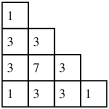
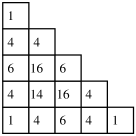
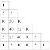
Figure 1. Triangular tables $T^{s}$ containing the numbers $V^{s}_{k,m}$. Southwest corners of these tables are located at $(0,0)$.

For a fixed $s$, we can arrange the numbers $V^{s}_{k,m}$ into a triangular table $T^{s}$ of size $s$ as shown on Figure 1. Namely, the number $V^{s}_{k,m}$ is placed into the cell, whose southwest (lower left) corner is at position $(k,m)$. The next table $T^{s+1}$ can be obtained from the table $T^{s}$ as follows. First, we add to every element of $T^{s}$ its south, west and southwest neighbors. Next, we add a line of cells, whose positions $(k,m)$ satisfy the equality $k+m=s$. In every cell of this line, we put the sum of the south and west neighbors. Note that, by construction, the boundary of every table $T^{s}$ consists of binomial coefficients.

Consider the generating function $G=G_{3}$ for the numbers $V_{k,\ell,m}$. The splitting of $G$ into homogeneous components can be obtained by expanding the function $G(xy,y,zy)$ into powers of $y$. We set

$$G(xy,y,zy)=\sum_{s=0}^{\infty}g_{s}(x,z)y^{s}$$

Then we have

$$g_{s}(x,z)=\sum_{k=0}^{s}\sum_{m=0}^{s-k}V^{s}_{k,m}x^{k}z^{m}.$$

Thus the coefficients of the polynomial $g_{s}$ are precisely elements of the table $T^{s}$. The recurrence relations on the numbers $V^{s}_{k,m}$ displayed above imply the following property of the generating functions $g_{s}$:

Proposition 4.1.

The polynomials $g_{s}$ satisfy the following recurrence relations:

$$g_{s+1}=(1+x+z)g_{s}+\tau_{\leqslant s}(xzg_{s}),$$

where the truncation operator $\tau_{\leqslant s}$ acts on a polynomial by removing all terms, whose degrees exceed $s$.

Consider the polynomials

$$h_{s}(x,z)=g_{s}(x,z)-(xz)^{s}g_{s}(z^{-1},x^{-1}).$$

Geometrically, these polynomials can be described as follows. Let $\tilde{T}^{s}$ denote the table, into which we put all coefficients of the polynomial $h_{s}$, see Figure 2. The lower left triangle of size $s-1$ is the same in the tables $T^{s}$ and $\tilde{T}^{s}$. The table $\tilde{T}^{s}$ is skew-symmetric with respect to the main diagonal. These two properties give a unique characterization of the tables $\tilde{T}^{s}$.

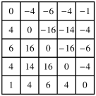
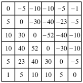
Figure 2. The skew-symmetric tables $\tilde{T}^{s}$.

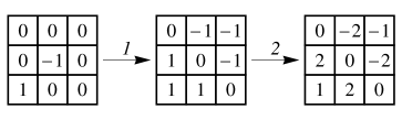
Figure 3. The rules of generating the tables $\tilde{T}^{s}$.

The rules, by which the tables $\tilde{T}^{s}$ are formed, are the following (see Figure 3). The first table $\tilde{T}^{1}$ is by definition the left-most table shown on Figure 2. The next table $\tilde{T}^{s+1}$ is obtained inductively from the preceding table $\tilde{T}^{s}$ in two steps. In the first step, we add to every element of $\tilde{T}^{s}$ its immediate west, south and southwest neighbors. In the second step, we modify elements in two diagonals of the table, namely, the elements, whose positions (mesured by southwest corners) $(k,m)$ satisfy the equality $k+m=s$ or $k+m=s+2$. To the cell at position $(k,m)$, where $k+m=s$, we add the binomial coefficient $\binom{k+m}{m}$. From the cell at position $(k+1,m+1)$, we subtract this binomial coefficient.

We have the following recurrence relation on the polynomials $h_{s}$:

$$h_{s+1}=h_{s}(1+x)(1+z)+(1-xz)(x+z)^{s},$$

which does not contain truncation operators. Therefore, the generating function $H=\sum_{s=0}^{\infty}h_{s}y^{s}$ satisfies the following linear equation:

$$H=1+y((1+x)(1+z)H+(1-xz)(1-y(x+z))^{-1}).$$

Solving this equation, we find that

$$H=\frac{y(1-xz)}{(1-y(x+z))(1-y(1+x)(1+z))}.$$

Knowing the generating function $H$, we can now obtain an explicit formula for the polynomials $h_{s}$, namely,

$$h_{s}(x,z)=\frac{1-xz}{1+xz}\left((1+x)^{s}(1+z)^{s}-(x+z)^{s}\right).$$

Theorem 1.4 is thus proved.

Open problems

1. Prove or disprove: the generating function $G_{4}$ is algebraic. Note that $G_{1}$ and $G_{2}$ are rational, and $G_{3}$ is algebraic.

2. Deduce differential or difference equations on the generating functions for the $f$-vectors and for the modified $h$-vectors of Gelfand–Zetlin polytopes.

References

[GZ]I.M.Gelfand, M.L.Cetlin,
Finite dimensional representations of the
group of unimodular matrices, Doklady Akad. Nauk USSR (N.S.), 71
(1950), 825–828
[KST]V. Kiritchenko, E. Smirnov, V. Timorin,
Schubert calculus and Gelfand–Zetlin polytopes, preprint
[O]A. Okounkov, A remark on the Hilbert polynomial of a spherical manifold, Funct. Anal. Appl. 31
(1997), no. 2, 138–140