Microscopic origin of the linear temperature increase of the magnetic susceptibility of BaFe₂As₂

Abstract

Employing a combination of ab initio band structure theory and dynamical mean-field theory we explain the experimentally observed linear temperature increase of the magnetic susceptibility of the iron pnictide material BaFe₂As₂. The microscopic origin of this anomalous behaviour is traced to a sharp peak in the spectral function located approximately 100 meV below the Fermi level. This peak is due to the weak dispersion of two-dimensional bands associated with the layered crystal structure of pnictides.

I INTRODUCTION

Since the discovery of high-temperature superconductivity in the iron pnictides Fepnic the unusual electronic properties of this class of materials has attracted considerable attention singhsdw ; rotter ; Wang ; klingeler ; korshunov ; zhang ; Aichhorn ; BaFe2As2 ; LaFePO10 ; arpes1 ; arpes2 ; skornyakov . The interest was stimulated by the fact that the new superconductors share several similarities with the well-studied, but still not well understood, high-$T_{c}$ cuprates. Firstly, both classes of superconductors crystallize into a layered structure. Secondly, in most cases the parent compounds of the pnictides are not superconducting, and superconductivity emerges only under doping or pressure and is associated with the suppression of antiferromagnetic (AFM) order. However, in contrast to the cuprates whose parent compounds are Mott insulators, the parent compounds of the pnictides are multiband metals. The nature of the magnetic ground state of the parent compounds is also different: in the cuprates it corresponds to a Néel-type order of a Mott-Hubbard insulator, while in the pnictides magnetism is associated with a nesting-induced spin density wavesinghsdw ; rotter ; delacruz (SDW).

The magnetic properties of pnictide materials show anomalous behavior even in the paramagnetic state. An unusual linear temperature increase of the uniform magnetic susceptibility was reported in the parent compound BaFe₂As₂Wang as well as in stoichiometric and fluorine-doped LaFeAsOklingeler . It is now well established that the linear increase of the magnetic susceptibility with temperature is a general property of all pnictide superconductors for temperatures above the SDW transition. Nevertheless, no consensus has been reached so far about the origin of this phenomenon. To date several mechanisms were proposed to explain the observed $T$-dependence in the pnictides. Wang et al.Wang and Zhang et al.zhang suggested that the linear-$T$ behavior is a consequence of strong antiferromagnetic fluctuations present above the SDW transition temperature. Korshunov et al. korshunov argued that short-range antiferromagnetic fluctuations are the source of a linear-$T$ term in the susceptibility of a two-dimensional Fermi liquid which allowed them to obtain good agreement with experimental data.

A very important issue concerning the spectral and magnetic properties of the pnictides is the role of Coulomb correlations. It is now generally accepted that electronic correlations in the pnictides are not as strong as in the cuprates and should be classified as moderateAichhorn ; BaFe2As2 . It was shownBaFe2As2 ; LaFePO10 that the spectral properties of the pnictides can be reproduced by first-principles techniques only if local dynamical Coulomb correlations are taken into account. This can be achieved by employing the LDA+DMFT methodLDApDMFT . This computational scheme combines electronic band structure calculations in the local density approximation (LDA) with many-body physics incorporated in the dynamical mean-field theory (DMFT)DMFT89 .

In our earlier studyskornyakov we proposed an explanation of the temperature increase of the magnetic susceptibility of LaFeAsO which was based on a first-principles analysis of the low-energy spectral properties caused by local dynamical Coulomb correlations, without taking into account interatomic magnetic fluctuations. In the present paper we employ the LDA+DMFT scheme to demonstrate that the proposed mechanism can be applied also to understand the origin of the linear temperature dependence of the uniform magnetic susceptibility in stoichiometric BaFe₂As₂.

II COMPUTATIONAL METHOD

The LDA+DMFT computational scheme implemented in the present work proceeds in four steps: (i) the construction of an effective tight-binding Hamiltonian $\hat{H}^{\rm WF}({\bf k})$ from a converged LDA solution by projectingproj onto Wannier functions, (ii) the addition of the local Coulomb interaction $\hat{H}^{\rm Coul}$, (iii) a double-counting correction which takes into account the local interactions already decribed by the LDA, and (iv) the self-consistent solution of the DMFT equations on the Matsubara contour with continuous-time quantum Monte-CarloCTQMC1 (CT-QMC) as impurity solver. The Hamiltonian to be solved by DMFT is given by

$$\hat{H}^{\rm DMFT}({\bf k})=\hat{H}^{\rm WF}({\bf k})+\hat{H}^{\rm Coul}+\hat{H}^{\rm DC}.$$ (1)

Exact investigations of the magnetic response of this model must employ a rotationally invariant form of the interaction term $\hat{H}^{\rm Coul}$. However, up to now there do not exist effective algorithms for the solution of a five-orbital Hubbard model with the full Coulomb interaction within CT-QMC. Furthermore, our investigation of the magnetic properties of BaFe₂As₂ requires a separate, and extremely time-consuming, self-consistent DMFT calculation for each point of the susceptibility curve. To make computations feasible, we therefore include only the density-density contributions to the full interaction

$$\hat{H}^{\rm Coul}\equiv\hat{H}^{\rm U}=\frac{1}{2}\sum_{i,\alpha,\alpha^{\prime},\sigma,\sigma^{\prime}}U^{\sigma\sigma^{\prime}}_{\alpha\alpha^{\prime}}\hat{n}_{i\alpha\sigma}^{d}\hat{n}_{i\alpha^{\prime}\sigma^{\prime}}^{d}.$$ (2)

Here $U^{\sigma\sigma^{\prime}}_{\alpha\alpha^{\prime}}$ is the Coulomb interaction matrix, $\hat{n}_{i\alpha\sigma}^{d}$ is the occupation number operator for $d$ electrons in the orbital $\alpha$ or $\alpha^{\prime}$, with spin $\sigma$ or $\sigma^{\prime}$, on the $i$th site. This approximation neglects spin flip and pair hopping processes. Nevertheless, as will be shown below, it is able to provide correct results for the spectral and magnetic properties of BaFe₂As₂. The double-counting term is $\hat{H}^{\rm DC}=-{\bar{U}}(n_{\rm DMFT}-\frac{1}{2})\hat{I}$, where $n_{\rm DMFT}$ is the total, self-consistently determined number of $d$ electrons obtained within LDA+DMFT, and $\bar{U}$ is the average Coulomb parameter for the $d$ shell.

We construct Wannier functions in the energy window including Fe-$d$ and As-$p$ states. Hence, by construction energy bands of the $H^{\rm WF}$ Hamiltonian exactly reproduce 16 Fe-$d$ and As-$p$ bands (two As and Fe atoms in the formula unit, one formula unit in the unit cell) obtained in LDA calculations, and the $p-d$ hybridization is explicitly taken into account.

The interaction matrix $U^{\sigma\sigma^{\prime}}_{\alpha\alpha^{\prime}}$ is parametrized by the effective on-site Coulomb parameter $U$ and intra-orbital exchange parameter $J$ according to the procedure described in Ref.UJCalculation . In the present calculation we use $U$=3.5 eV and $J$=0.85 eV obtained with the constrained DFT procedureConstrainedDFT1 ; ConstrainedDFT2 ; ConstrainedDFT3 .

The orbitally resolved spectral functions of the interacting system are then computed as

$$A_{\alpha}(\omega)=-\frac{1}{\pi}\mathrm{Im}\sum_{{\mathbf{k}}}[(\omega+\mu)\hat{I}-\hat{H}^{\mathrm{WF}}(\mathbf{k})-\hat{H}^{\mathrm{DC}}-\hat{\Sigma}(\omega)]_{\alpha\alpha}^{-1},$$

where the subscript $\alpha$ refers to an orbital, $\mu$ is the self-consistent chemical potential, and $\Sigma(\omega)$ is the self-energy on the real axis obtained by analytic continuation using the Padé approximantPade1 technique; details are described in Ref.LaFePO10 .

The uniform magnetic susceptibility is calculated as the response of the system to a weak external magnetic field,

$$\chi(T)=\frac{\partial M(T)}{\partial E_{h}}=\frac{\partial[n_{\uparrow}(T)-n_{\downarrow}(T)]}{\partial E_{h}},$$

where $M(T)$ is the field-induced magnetization, $n_{\sigma}(T)$ is the number of electrons with spin $\sigma$, and $E_{h}$ is the energy correction corresponding to the applied field. Since the field is finite the calculations are performed in three steps: First, we check that the polarization is zero in the absence of the field, then we check that $M(T)$ is a linear function of $E_{h}$, and finally we evaluate the derivative in Eq. (II) as a ratio of $M(T)$ and $E_{h}$.

III RESULTS

III.1 Temperature dependence of the uniform magnetic susceptibility

In Fig. 1 the uniform magnetic susceptibility $\chi(T)$ computed within LDA+DMFT is compared with the experimental data of Wang et al.Wang . In the temperature range from 200 K to 600 K the temperature dependence of the calculated $\chi(T)$ is found to be almost perfectly linear. However, the slope is by a factor of 1.7 smaller than in the experiment. The origin of this quantitative discrepancy is not clear at the moment and will be the subject of future investigations. To emphasize the linearity we plot a least-square fit to the last six points of the computed data. We note that the observed linear behavior is, in fact, due to an extended linear region around the turning point of $\chi(T)$ at $\approx$350 K. The obtained $\chi(T)$ has a maximum at about 1000 K and decreases for higher temperatures.

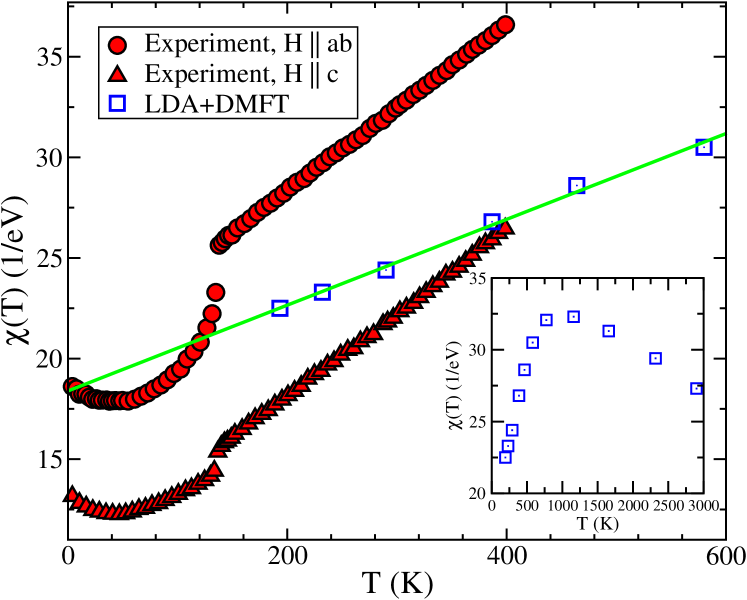
Figure 1: (Color online) Uniform magnetic susceptibility $\chi(T)$ of BaFe₂As₂ calculated within LDA+DMFT (squares) in comparison with experimental data of Wang et al.Wang (circles and triangles). The line is a least-square fit to the last six points of the computed data. The inset shows the theoretical curve for the full temperature interval.

More detailed information about the magnetic properties of BaFe₂As₂ can be obtained from an analysis of the orbitally resolved contributions $\chi_{\alpha}(T)$ ($\alpha=xy$, $yz$, $xz$, $3z^{2}-r^{2}$, $x^{2}-y^{2}$) to the total magnetic susceptibility. In Fig. 2 we show the temperature dependence of the Fe 3$d$ susceptibilities of BaFe₂As₂ obtained in LDA+DMFT. All contributions have approximately equal slope in the temperature interval from 200 K to 500 K. The $d_{xy}$ orbital of Fe provides the largest contribution to the total susceptibility.

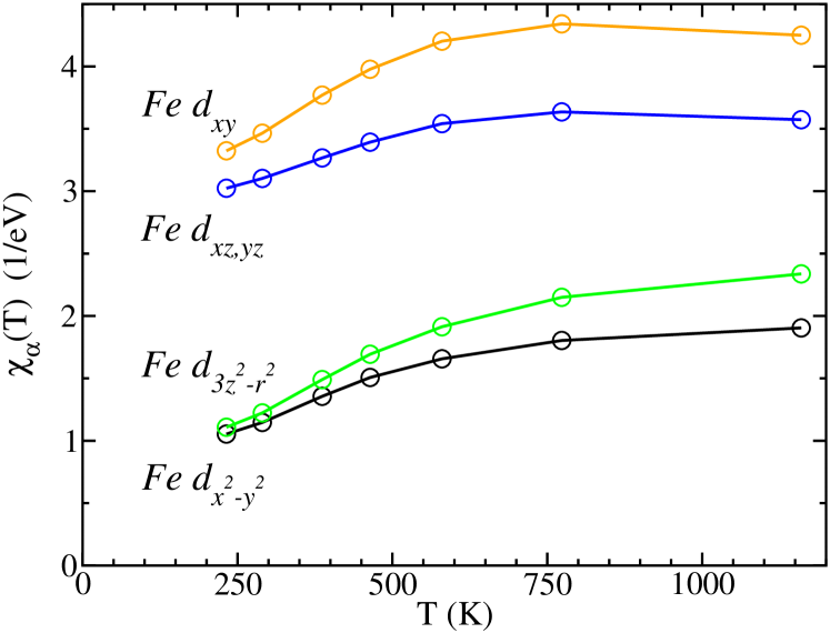
Figure 2: (Color online) LDA+DMFT results for the orbitally resolved Fe 3$d$ susceptibilities $\chi_{\alpha}(T)$ with $\alpha=xy$, $yz$, $xz$, $3z^{2}-r^{2}$, $x^{2}-y^{2}$ of BaFe₂As₂ vs. temperature obtained from the derivative of the magnetization.

III.2 Connection between magnetic and spectral properties

In our previous paperskornyakov we proposed a scenario according to which the anomalous $T$-behavior of $\chi(T)$ in the pnictides is connected with the presence of a sharp peak in the spectral function below the Fermi energy. In Fig. 3 the total Fe 3$d$ spectral function $A(\omega)$ computed within LDA+DMFT is shown in comparison with the LDA result. It demonstrates that dynamical correlation effects strongly renormalize the spectrum in the vicinity of the Fermi energy. In particular, the electronic correlations are seen to lead to a narrow peak below the Fermi level while the remaining part of the spectrum is only weakly affected by the correlations. The peak in the energy window from -4 eV to -2 eV should not be mistaken for a lower Hubbard band since a similar peak is already present in the LDA result. The Fe 3$d$ spectral weight in this energy area is a consequence of the hybridization with As 4$p$ states.

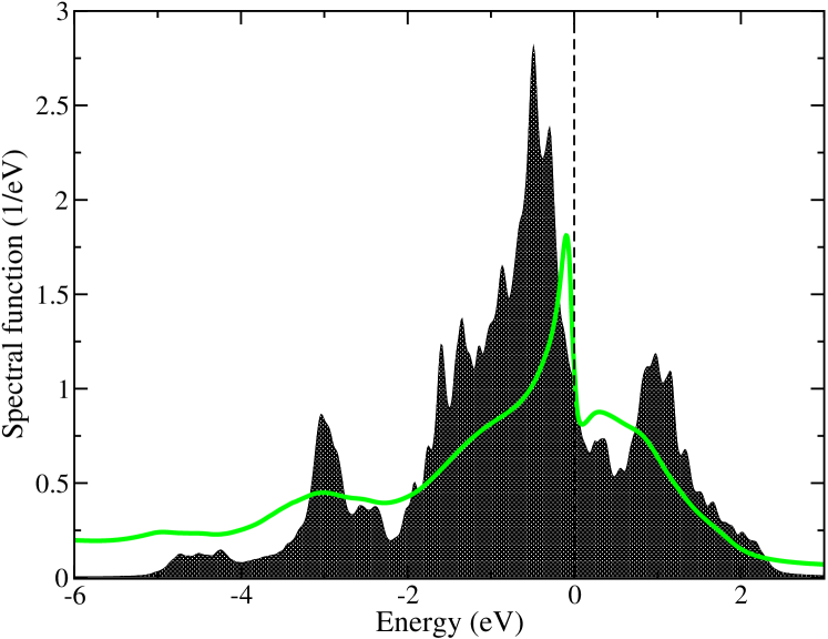
Figure 3: (Color online) Comparison of the total Fe 3$d$ spectral function of BaFe₂As₂ as obtained from LDA+DMFT (solid line) and LDA (shaded area), respectively.

A comparison of the orbitally resolved spectral functions computed within LDA and LDA+DMFT, respectively, is shown in Fig. 4. The LDA+DMFT results are in good agreement with previously reported theoretical and experimental spectra BaFe2As2 . Except for the $d_{x^{2}-y^{2}}$ orbital the spectral functions obtained by LDA+DMFT all show a sharp peak below the Fermi energy. These peaks originate from local correlation effects as pointed out above.

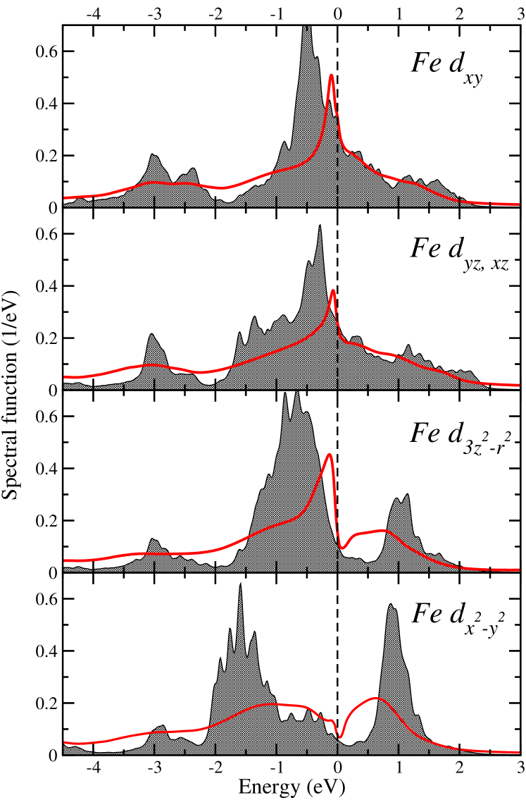
Figure 4: (Color online) Orbitally resolved Fe 3d spectral functions of BaFe₂As₂ obtained within LDA+DMFT (solid lines) in comparison with LDA results (filled areas). The Fermi energy is set to 0 eV.

A quantitative measure of the correlation strength is the quasiparticle renormalization factor $Z$. In the single-orbital case it can be obtained from the real-axis self-energy $\Sigma(\omega)$ which is related to the effective mass enhancement $m^{*}/m$ by $Z^{-1}=1-\partial Re(\Sigma(\omega))/\partial\omega=m^{*}/m$. For a multi-orbital problem the self-energy is a matrix. Therefore different orbitals have different $m^{*}/m$. The computed values of the mass enhancement range from 2.5 to 3.7 and agree well with previous estimates of $m^{*}/m$ for pnictides obtained from the renormalization of the LDA band structure Aichhorn ; BaFe2As2 ; LaFePO10 ; arpes1 ; arpes2 .

To identify possible reasons for the anomalous behavior of the magnetic properties it is instructive to compute the temperature evolution of the orbitally resolved spectral functions. The spectral curves computed for temperatures ranging from 232 K to 580 K are shown in Fig. 5.

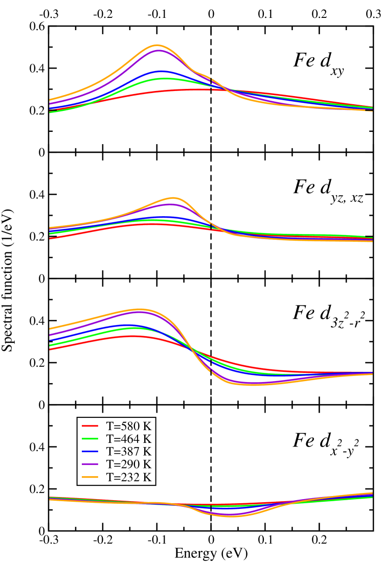
Figure 5: (Color online) Fe 3d spectral functions of BaFe₂As₂ computed within LDA+DMFT in the temperature range 232 K - 580 K. The Fermi energy corresponds to 0 eV.

All spectral functions, except for the $d_{x^{2}-y^{2}}$ orbital, show a temperature sensitive peak which is located approximately 100 meV below the Fermi energy. These peaks increase in amplitude and become narrow with decreasing $T$. We note that the magnitudes of the orbital contribution $\chi_{\alpha}(T)$ are proportional to the density of states of the corresponding orbitals at the Fermi energy.

The simplest way to establish a possible connection between the temperature evolution of the magnetic susceptibility and the excitation spectrum in the multi-orbital case is to estimate the susceptibility (per spin) using the bubble diagram obtained by convoluting the DMFT Green’s functions, Eq. (3),

$${\chi}^{0}_{\alpha}(T)=\frac{1}{\beta}\sum_{\mathbf{k,}i\omega,\alpha^{\prime}}\hat{G}_{\alpha\alpha^{\prime}}(\mathbf{k},i\omega)\hat{G}_{\alpha^{\prime}\alpha}(\mathbf{k},i\omega),$$ (3)

where $\hat{G}_{\alpha\alpha^{\prime}}(\mathbf{k},i\omega)=[(i\omega+\mu)\hat{I}-\hat{H}^{\mathrm{DMFT}}(\mathbf{k})-\hat{\Sigma}(i\omega)]_{\alpha\alpha^{\prime}}$. This expression describes the spin susceptibility in the absence of vertex corrections, i.e., gives an estimate of the magnetic response due to single-particle excitations which are characterized by the interacting spectral function. An explicit connection between the magnetic response, Eq. (3), with the excitation spectrum can be made in the one-orbital case when off-diagonal elements of $\hat{G}$ are absent:

$$\chi_{1}(T)=-\frac{1}{4\pi^{2}}\int d\omega_{1}d\omega_{2}\frac{f_{\mathrm{F}}(\omega_{1})-f_{\mathrm{F}}(\omega_{2})}{\omega_{1}-\omega_{2}}A(\omega_{1})A(\omega_{2}).$$ (4)

Here $A(\omega)$ is the spectral function of the interacting system(per spin), and the temperature enters via the Fermi function, $f_{\mathrm{F}}(\omega)$. In real compounds multi-orbital physics, including hybridization effects, is important, in which case the full matrix Green functions must be used in Eq. (3).

The influence of interaction effects may be estimated by calculating the magnetic susceptibility in the random-phase approximation (RPA). If the orbital dependence of the Coulomb interaction between $d$ electrons is neglected, the orbital contributions to the total uniform $d$ magnetic susceptibility within RPA are given by

$$\chi^{\mathrm{RPA}}_{\alpha}(T)=\frac{2\chi^{0}_{\alpha}(T)}{1-{\bar{U}}\chi^{0}_{\alpha}(T)},$$ (5)

where the factor 2 is due to the spin degeneracy. The temperature dependence of the orbitally resolved susceptibilities computed according to Eq. (5), is shown in Fig. 6. For the $d_{3z^{2}-r^{2}}$ and $d_{x^{2}-y^{2}}$ orbitals the results are in good qualitative agreement with the full LDA+DMFT solution. By contrast, the temperature dependence of the susceptibilities corresponding to the $d_{xy}$, $d_{yz}$, and $d_{xz}$ states is not reproduced by Eq. (5); apparently vertex corrections are important in this case.

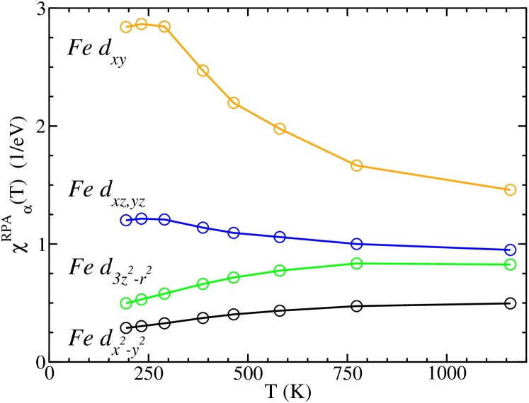
Figure 6: (Color online) LDA+DMFT results for the orbitally resolved Fe 3$d$ susceptibilities $\chi^{\mathrm{RPA}}_{\alpha}(T)$ with $\alpha=xy$, $yz$, $xz$, $3z^{2}-r^{2}$, $x^{2}-y^{2}$ of BaFe₂As₂ vs. temperature, obtained from the RPA expression for the susceptibility in Eq. (5).

The above results suggest the following interpretation, whose correctness will be demonstrated later: The electronic states forming the sharp peak in the spectral function below the Fermi energy lead to thermal excitations which contribute to the susceptibility. When the energy $k_{\mathrm{B}}T$ is larger than the distance between the peak and the Fermi level, the number of states which can be excited is reduced and the susceptibility starts to decrease. A more complex mechanism is responsible for the increase of the $d_{x^{2}-y^{2}}$ susceptibility where the corresponding spectral function does not show a peak below the Fermi energy.

Namely, as in the case of LaFeAsOskornyakov the off-diagonal contributions to the susceptibility, $\chi^{0}_{\alpha\alpha^{\prime}}=1/\beta\sum_{\mathbf{k,}i\omega}\hat{G}_{\alpha\alpha^{\prime}}(\mathbf{k},i\omega)\hat{G}_{\alpha^{\prime}\alpha}(\mathbf{k},i\omega)$, and in particular $\chi^{0}_{x^{2}-y^{2},3z^{2}-r^{2}}(T)$, are responsible for the increase of $\chi_{x^{2}-y^{2}}^{0}(T)$. Thus the temperature increase of $\chi^{\mathrm{RPA}}_{x^{2}-y^{2}}(T)$ is caused by the magnetic response of the other orbitals (for details see the supplementary material of Ref.skornyakov ). A detailed analysis of the proposed mechanism of the increase of $\chi(T)$ using a simplified model will be presented in the following section.

III.3 Model analysis

To further clarify the relation between the shape of the spectral function and the anomalous temperature behavior of the magnetic properties we will now perform a model calculation, where multi-orbital effects are neglected. As a first step we compute the DMFT spin susceptibility for a single-band model, constructed in such a way that the non-interacting system has exactly the same spectral function as the one for the $d_{xy}$ orbital of the tight-binding Hamiltonian $H_{\mathrm{WF}}$ in Eq. (1). In the upper panel of Fig. 7 the temperature dependence of the spin susceptibility computed for the model within DMFT is shown for several values of the chemical potential. The corresponding spectral functions of the interacting system are presented in the inset of Fig. 7.

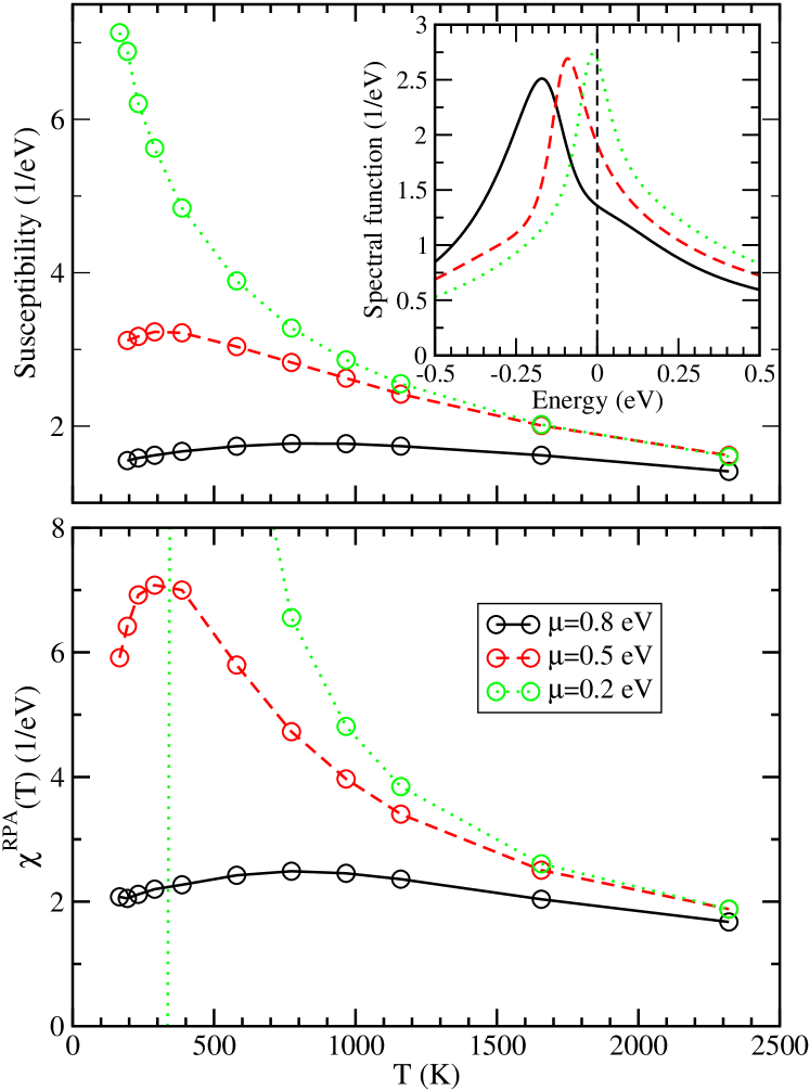
Figure 7: (Color online) LDA+DMFT results for the uniform magnetic susceptibility of a one-band model with the non-interacting Fe $d_{xy}$ DOS of BaFe₂As₂ as a function of temperature. Upper panel: Results computed according to Eq. (II); the inset shows the spectral function of the interacting system. Lower panel: RPA results for the uniform magnetic susceptibility using Eq. (5); the divergence of the susceptibility for $\mu$=0.2 eV at about 300 K is an artifact of the RPA.

Depending on the peak position there are two characteristically different temperature dependencies of the susceptibility: (i) an increase in the low temperature region with a maximum at an intermediate temperature followed by a decrease at higher $T$ ($\mu$=0.5 eV, 0.8 eV), and (ii) a monotonic decrease with temperature ($\mu$=0.2 eV). The former regime is obtained when the peak is substantially below the Fermi energy, the latter regime corresponds to the case when the peak is very close to, or right at, the Fermi energy. The result of the estimate of the susceptibility according to Eq. (5) is presented in the lower panel of Fig. 7. It is seen to reproduce all features of the curves computed by Eq. (II).

This confirms that the magnetic response of the system is indeed governed by its spectral properties. Thus, the driving force of the non-monotonic behavior of the susceptibility is the peak below the Fermi energy. In particular, the distance between the peak and the Fermi level is important. In spite of the fact that the peak in the spectral function exists at the level of LDA, its position is too far from the Fermi energy to cause a serious increase of the susceptibility. The correlations shift the peak towards the Fermi level which results in more pronounced temperature dependence of $\chi(T)$.

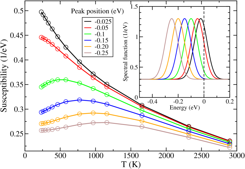
Figure 8: (Color online) Spin susceptibility $\chi_{1}(T)$ of a model defined by the density of states (6) calculated from Eq. (4) for different values of the peak position. The inset shows the density of states plotted relative to the Fermi energy (zero energy).

To relate the shape of the spectral function with the two temperature regimes of the magnetic susceptibility even more explicitly, we now compute the temperature behavior of $\chi^{0}(T)$ for a system with a density of states given by a Gauss function with offset from the energy axis,

$$A(\omega)=A+B\exp[(\frac{\omega-C}{2\sigma})^{2}].$$ (6)

The parameters in Eq. (6) were adjusted such that the maximum and the width of the function are close to the ones obtained with LDA+DMFT for the material specific Hamiltonian for BaFe₂As₂. Results for $\chi_{1}(T)$ computed according to Eq. (4) are shown in Fig. 8. The temperature behavior of $\chi_{1}(T)$ and its evolution upon changes of the peak position in the spectral function are seen to qualitatively reproduce all features obtained in DMFT for the one-band model. This can be viewed as a direct indication that the peculiarities observed in the anomalous behavior of the spin susceptibility in DMFT originate from the shape of the spectral function in the vicinity of the Fermi energy.

Finally we address the question concerning the microscopic origin of the peaks in the spectral function below the Fermi level. In the following analysis we focus on the $d_{xy}$ orbital since the peak in its spectral function is sharper than those of the other orbitals. The contributions of the $d_{xy}$ states to the band structure are shown in the left upper panel of Fig. 9 as ”fat bands” (i.e., the thickness of a band is proportional to the contribution of states with selected symmetry). The peak in the $d_{xy}$ spectral function (Fig. 9, right upper panel) is formed by regions of relatively flat bands centered at the energy approximately -0.4 eV relative to the Fermi level.

To construct a minimal model describing the energy dispersion of the $d_{xy}$ states we solve an effective two-band Hamiltonian $H^{2D}({\bf k})$ with two Fe atoms in the unit cell, which is obtained from a projection of Bloch states in the vicinity of the Fermi energy onto a subspace of Wannier functions with $d_{xy}$ symmetry. The energy bands of $H^{2D}({\bf k})$ are shown in the left upper panel of Fig. 9 by solid curves. In the next step we introduce the real-space Hamiltonian $H^{2D}_{real}$ written for a square lattice with two atoms in the unit cell and nonzero hoppings within three coordinate spheres. The Hamiltonian $H^{2D}_{real}$ has the form

$$H^{2D}_{real}=t\sum_{i{\mathbf{R}}}c^{\dagger}_{i\mathbf{R}}c_{i}+t^{\prime}\sum_{i{\mathbf{R}}^{\prime}}c^{\dagger}_{i{\mathbf{R}}^{\prime}}c_{i}+t^{\prime\prime}\sum_{i{\mathbf{R}}^{\prime\prime}}c^{\dagger}_{i{\mathbf{R}}^{\prime\prime}}c_{i},$$ (7)

where $i$ labels the atoms, and the radius vectors ${\mathbf{R}}$, ${\mathbf{R}}^{\prime}$ and ${\mathbf{R}}^{\prime\prime}$ correspond to the cluster of nearest, next-nearest and next-next-nearest neighbors, respectively, around atom $i$. The hopping parameters $t$=-170 meV, $t^{\prime}$=98 meV and $t^{\prime\prime}$=21 meV were computed as Fourier transforms of the material-specific Hamiltonian $H^{2D}({\bf k})$.

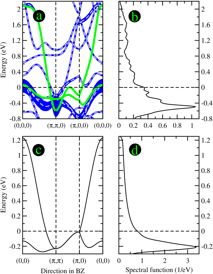
Figure 9: (Color online) Band structure and spectral functions computed for BaFe₂As₂; the Fermi energy corresponds to 0 eV. (a) Dispersion curves calculated within LDA (dashed curves), contributions of the orbitals with $d_{xy}$ symmetry (fat bands), energy bands of a two-orbital model obtained as a projection onto the $d_{xy}$ states (solid curves). (b) Spectral function of the $d_{xy}$ orbital from LDA. (c) Energy bands of a model corresponding to the real hopping parameters. (d) Spectral function of the model Hamiltonian (7).

The shape of the energy bands and the spectral function computed for Hamiltonian (7) are shown in the lower panels of Fig. 9. They are in good agreement with the corresponding characteristics obtained from the direct calculation. As in the multi-orbital case, the band structure of (7) represents a combination of dispersive bands and bands with less pronounced ${\bf k}$-dependence. In particular, it follows that the peak below the Fermi energy is formed by a relatively flat band located in the same energy interval as the peak.

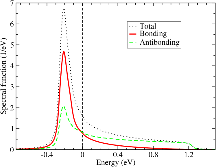
Figure 10: (Color online) Spectral functions of Hamiltonian (7) calculated in the basis of bonding (solid curve) and antibonding (dashed curve) wave functions. The total spectral function is shown by a dotted line. The Fermi energy is set to zero.

In order to understand the coexistence of the flat and dispersive regions within a band of given symmetry ($d_{xy}$ in our case) it is instructive to plot the spectral functions of the Hamiltonian (7) in the basis of bonding and antibonding wave functions. In other words, if $\left|\phi_{1}\right>$ is the wave function on the one atom in the unit cell, $\left|\phi_{2}\right>$ is the wave function of the other atom. Then the new basis is defined as $\left|\phi_{+}\right>=\left|\phi_{1}\right>+\left|\phi_{2}\right>$ and $\left|\phi_{-}\right>=\left|\phi_{1}\right>-\left|\phi_{2}\right>$. Spectral functions of the Hamiltonian (7) computed for that basis with realistic hopping parameters and chemical potential are shown in Fig. 10. From Fig. 10 it follows that the band with a pronounced dispersion is mainly formed by antibonding linear combination $\left|\phi_{-}\right>$ and the main contribution to the peak is provided by the bonding function $\left|\phi_{+}\right>$ whose dispersion is less pronounced.

IV CONCLUSIONS

By employing the LDA+DMFT method we investigated the interplay between the spectral and magnetic properties of BaFe₂As₂. The calculated temperature dependence of the uniform magnetic susceptibility is in good agreement with experimental data. Our calculations show that there are pronounced, temperature sensitive peaks below the Fermi energy in the spectral function of BaFe₂As₂. We proposed a scenario according to which the temperature increase of the susceptibility is a consequence of the thermal excitation of the electronic states which lead to these peaks. Our analysis is based on the DMFT solution of a one-band model with a density of states corresponding to the Fe-$d_{xy}$ spectral function of BaFe₂As₂. The results clearly demonstrate that the peak in the spectral function in the vicinity of the Fermi energy is a prerequisite for the linear temperature increase of magnetic susceptibility. The peaks in the real compound are due to the weak dispersion of bonding states arising from the layered structure of BaFe₂As₂.

V ACKNOWLEDGMENTS

The authors thank P. Werner and J. Kuneš for supplying us with the CT-QMC code used in our calculations, and X.H. Chen for providing the experimental data in digitalized form. This work was supported by the Russian Foundation for Basic Research (Projects No. 10-02-00046-a, No. 10-02-96011-r_ural_a, No. 12-02-91371-CT_a). S.L.S. is grateful to the Dynasty Foundation for support. S.L.S and V.I.A. are grateful to the Center for Electronic Correlations and Magnetism, University of Augsburg for hospitality. This work was supported in part by the Deutsche Forschungsgemeinschaft through Transregio TRR 80.

References

- (1) Y. Kamihara, H. Hiramatsu, M. Hirano, R. Kawamura, H. Yanagi, T. Kamiya, and H. Hosono, J. Am. Chem. Soc. 128, 10012 (2006); Y. Kamihara, T. Watanabe, M. Hirano, and H. Hosono, J. Am. Chem. Soc. 130, 3296 (2008); Z.-A. Ren, W. Lu, J. Yang, W. Yi, X.-L. Shen, Z.-C. Li, G.-C. Che, X.-L. Dong, L.-L. Sun, F. Zhou, and Z.-X. Zhao, Chin. Phys. Lett. 25, 2215 (2008).
- (2) D. J. Singh, Physica C 469, 418 (2009).
- (3) M. Rotter, M. Tegel, D. Johrendt, I. Schellenberg, W. Hermes, R. Pottgen, Phys. Rev. B 78, 020503 (2008).
- (4) C. de la Cruz, Q. Huang, J. W. Lynn, J. Li, W. Ratcliff, J. L. Zarestzky, H. A. Mook, G. F. Chen, J. L. Luo, N. L. Wang, and P. Dai, Nature, 453, 899 (2008).
- (5) X. F. Wang, T. Wu, G. Wu, H. Chen, Y. L. Xie, J. J. Ying, Y. J. Yan, R. H. Liu, and X. H. Chen, Phys. Rev. Lett. 102, 117005 (2009).
- (6) R. Klingeler, N. Leps, I. Hellmann, A. Popa, U. Stockert, C. Hess, V. Kataev, H.-J. Grafe, F. Hammerath, G. Lang, S. Wurmehl, G. Behr, L. Harnagea, S. Singh, and B. Büchner, Phys. Rev. B 81, 024506 (2010).
- (7) G. M. Zhang, Y. H. Su, Z. Y. Lu, Z. Y. Weng, D. H. Lee, and T. Xiang, Europhys. Lett. 86, 37006 (2009).
- (8) M. M. Korshunov, I. Eremin, D. V. Efremov, D. L. Maslov, and A. V. Chubukov, Phys. Rev. Lett. 102, 236403 (2009).
- (9) M. Aichhorn, L. Pourovskii, V. Vildosola, M. Ferrero, O. Parcollet, T. Miyake, A. Georges, and S. Biermann, Phys. Rev. B 80, 085101 (2009).
- (10) S. L. Skornyakov, A. V. Efremov, N. A. Skorikov, M. A. Korotin, Yu. A. Izyumov, V. I. Anisimov, A. V. Kozhevnikov, and D. Vollhardt, Phys. Rev. B 80, 092501 (2009).
- (11) S. L. Skornyakov, N. A. Skorikov, A. V. Lukoyanov, A. O. Shorikov, and V. I. Anisimov, Phys. Rev. B 81, 174522 (2010).
- (12) V. I. Anisimov, A. I. Poteryaev, M. A. Korotin, A. O. Anokhin and G. Kotliar, J. Phys.: Condens. Matter 9 7359 (1997); K. Held, I. A. Nekrasov, G. Keller, V. Eyert, N. Blümer, A. K. McMahan, R. T. Scalettar, T. Pruschke, V. I. Anisimov and D. Vollhardt, Phys. Status Solidi B 243 2599 (2006).
- (13) W. Metzner and D. Vollhardt, Phys. Rev. Lett. 62, 324 (1989).
- (14) S. L. Skornyakov, A. A. Katanin, and V. I. Anisimov, Phys. Rev. Lett. 106, 047007 (2011).
- (15) V. I. Anisimov, D. E. Kondakov, A. V. Kozhevnikov, I. A. Nekrasov, Z. V. Pchelkina, J. W. Allen, S.-K. Mo, H.-D. Kim, P. Metcalf, S. Suga, A. Sekiyama, G. Keller, I. Leonov, X. Ren, and D. Vollhardt, Phys. Rev. B 71, 125119 (2005).
- (16) P. Werner, A. Comanac, L. de’ Medici, M. Troyer, and A. J. Millis, Phys. Rev. Lett. 97, 076405 (2006).
- (17) A. I. Liechtenstein, V. I. Anisimov, J. Zaanen, Phys. Rev. B 52, R5467 (1995).
- (18) P. H. Dederichs, S. Blügel, R. Zeller, and H. Akai, Phys. Rev. Lett. 53, 2512 (1984).
- (19) O. Gunnarsson, O. K. Andersen, O. Jepsen, and J. Zaanen, Phys. Rev. B 39, 1708 (1989).
- (20) V. I. Anisimov and O. Gunnarsson, Phys. Rev. B 43, 7570 (1991).
- (21) H. J. Vidberg and J. W. Serene, J. Low Temp. Phys. 29, 179 (͑1977).
- (22) D. H. Lu, M. Yi, S.-K. Mo, A. S. Erickson, J. Analytis, J.-H. Chu, D. J. Singh, Z. Hussain, T. H. Geballe, I. R. Fisher, and Z.-X. Shen, Nature London 455, 81 (2008); D. H. Lu, M. Yi, S.-K. Mo, J. G. Analytis, J.-H. Chu, A. S. Erickson, D. J. Singh, Z. Hussain, T. H. Geballe, I. R. Fisher, and Z.-X. Shen, Physica C 469, 452 (2009).
- (23) S. V. Borisenko, V. B. Zabolotnyy, D. V. Evtushinsky, T. K. Kim, I. V. Morozov, A. N. Yaresko, A. A. Kordyuk, G. Behr, A. Vasiliev, R. Follath, and B. Büchner, Phys. Rev. Lett. 105, 067002 (2010).