Gravity, strings, modular and quasimodular forms

Abstract

Modular and quasimodular forms have played an important role in gravity and string theory. Eisenstein series have appeared systematically in the determination of spectrums and partition functions, in the description of non-perturbative effects, in higher-order corrections of scalar-field spaces, …The latter often appear as gravitational instantons i.e. as special solutions of Einstein’s equations. In the present lecture notes we present a class of such solutions in four dimensions, obtained by requiring (conformal) self-duality and Bianchi IX homogeneity. In this case, a vast range of configurations exist, which exhibit interesting modular properties. Examples of other Einstein spaces, without Bianchi IX symmetry, but with similar features are also given. Finally we discuss the emergence and the role of Eisenstein series in the framework of field and string theory perturbative expansions, and motivate the need for unravelling novel modular structures.

To appear in the proceedings of the Besse Summer School on Quasimodular Forms – 2010.

1 Introduction

Modular forms often appear in physics as a consequence of duality properties. This comes either as an invariance of a theory or as a relationship among two different theories, under some discrete transformation of the parameters. The latter transformation can be a simple $\mathbb{Z}_{2}$ involution or an element of some larger group like $SL(2,\mathbb{Z})$. The examples are numerous and have led to important developments in statistical mechanics, field theory, gravity or strings.

One of the very first examples, encountered in the 19th century, is the electrtic–magnetic duality in vacuum Maxwell’s equations (see e.g. [1]), which are invariant under interchanging electric and magnetic fields. This was revived in the more general framework of Abelian gauge theories by Montonen and Olive in 1977 [2] and culminated in the Seiberg–Witten duality in supersymmetric non-Abelian gauge theories [3]. There the duality group $SL(2,\mathbb{Z})$ acts on a complex parameter $\tau=\frac{\theta}{2\pi}+\frac{4\pi i}{g^{2}}$, where $\theta$ is the vacuum angle and $g$ is the coupling constant. The modular transformations give thus access to the non-perturbative regime of the field theory.

In statistical mechanics, the Kramers–Wannier duality [4] predicted in 1941 the existence of a critical temperature $T_{c}$ separating the ferromagnetic ($T<T_{c}$) and the paramagnetic ($T>T_{c}$) phases in the two-dimensional Ising model. The canonical partition function of the model, computed a few years later by Lars Onsager [5], is indeed expressed in terms of modular forms.

Over the last 30 years, modular and quasimodular forms have mostly emerged in the framework of gravity and string theory. At the first place, one finds (see e.g. [6]) the canonical partition function of a string of fundamental frequency $\omega$ at temperature $T$:

$$Z=\frac{1}{\eta(q)},$$ (1.1)

where $q=\exp 2i\pi z=\exp-\nicefrac{{\hbar\omega}}{{kT}}$ and $\eta(q)$ the Dedekind function (we refer to the appendix for definitions and conventions on theta functions, (A.1)–(A.5)). The average energy stored in a string at temperature $T$ is thus

$$\langle E\rangle=-\frac{\partial\ln Z}{\partial\nicefrac{{1}}{{kT}}}=\frac{\hbar\omega}{24}E_{2}(z),$$ (1.2)

where $E_{2}(z)$ the weight-two quasimodular form. Again, the modular properties of these functions translate into a low-temperature/high-temperature duality, which exhibits a critical temperature, signature of the Hagedorn transition.

In the above examples the modular group acts on a modular parameter related to the temperature. There is a plethora of examples in gravity and string theory of more geometrical nature, related to gravitational configurations and in particular to instantons.

An instanton is a solution of non-linear field equations resulting from an imaginary-time i.e. Euclidean action $S[\phi]$ as

$$\frac{\delta S}{\delta\phi}=0.$$ (1.3)

It should not to be confused with a soliton. The latter is a finite-energy solution of non-linear real-time equations of motion and appear in a large palette of phenomena such as the propagation of solitary waves in liquid media (as e.g. tsunamis) or black holes in gravitational set ups.

Instantons have finite action and enter the description of quantum-mechanical processes, which are not captured by perturbative expansions, as their magnitude is controlled by $\exp-\nicefrac{{1}}{{g}}$ at small coupling $g$ (in electrodynamics $g=\nicefrac{{e^{2}}}{{\hbar c}}$). These phenomena include quantum-mechanical tunneling and, more generally, decay and creation of bound states. Their amplitude is weighted by $\exp(-\nicefrac{{S}}{{\hbar}})$, where $S$ is the action of the instanton solution interpolating between initial and final configurations (see [8] for a pedagogical presentation of these methods).

All interacting (i.e. non-linear) field theories exhibit instantons. These emerged originally in Yang–Mills theories [9, 10] as well as in general relativity [11, 12, 13]. In the latter case, their usefulness for the description of quantum transitions is tempered by quantum inconsistencies of general relativity. Such configurations turn out nevertheless to be instrumental in modern theories of gravity, supergravity and strings for at least two reasons.

At the first place, some gravitational instantons falling in the class of asymptotically locally Euclidean (ALE) spaces have the required properties to serve as compactification set ups for superstring models usually defined in space–time of dimensions 10. This is the case, for example, of the Eguchi–Hanson gravitational instanton [12, 13], which appears as a blow-up of the $\mathbb{C}_{2}/\mathbb{Z}_{2}$ $A_{1}$-type singularity, or of more general Gibbons–Hawking multi-instantons [14].

The second reason is that supergravity and string theories contain many scalar fields called moduli. Their dynamics is often encapsulated in non-linear sigma models, which happen to have as a target space certain gravitational instantons such as the Taub-NUT, Atiyah–Hitchin, Fubini–Study, Pedersen or Calderbank–Pedersen spaces [11, 15, 16, 17, 18, 19, 20, 21]. Due to some remarkable underlying duality properties, most of the spaces at hand are expressed in terms of (quasi) modular forms, and this makes them relevant in the present context.

It should be finally stressed that in the framework of string and supergravity theories, quasimodular forms do not appear exclusively via compactification or moduli spaces. Recent developments on the perturbative expansions in quantum field theory reveal how relevant the spaces of quasimodular forms are for understanding the ultraviolet behaviour and its connections with string theory acting as a ultraviolet regulator[22]. They also call for introducing new objects, which stand beyond the realm of Eisenstein series [23].

2 Solving Einstein’s equations

It is a hard task in general to solve Einstein’s equations. In four dimensions with Euclidean signature, following the paradigm of Yang–Mills, the requirement of self-duality (or of a conformal variation of it) often leads to integrable equations. Those are in most cases related to self-dual Yang–Mills reductions, and possess remarkable solutions (see. e.g. [24]). It should be mentioned for completeness that self-duality can also serve as a tool in more than four dimensions. In seven or eight dimensions, it can be implemented using $G_{2}$ or quaternionic algebras [25, 26, 27, 28]. It is not clear, at present, whether in those cases some interesting and non-trivial relationship with quasimodular forms emerge. We will therefore not pursue this direction here.

2.1 Curvature decomposition in four dimensions

The Cahen–Debever–Defrise decomposition, more commonly known as Atiyah–Hitchin–Singer [29, 30], is a convenient taming of the 20 independent components of the Riemann tensor. In Cartan’s formalism, these are captured by a set of curvature two-forms ($a,b,\ldots=1,\ldots,4$)

$$\mathcal{R}^{a}_{\hphantom{a}b}=\mathrm{d}\omega^{a}_{\hphantom{a}b}+\omega^{a}_{\hphantom{a}c}\wedge\omega^{c}_{\hphantom{c}b}=\frac{1}{2}R^{a}_{\hphantom{a}bcd}\theta^{c}\wedge\theta^{d},$$ (2.1)

where $\left\{\theta^{a}\right\}$ are a basis of the cotangent space and $\omega^{a}_{\hphantom{a}b}=\Gamma^{a}_{\hphantom{a}bc}\theta^{c}$ the set of connection one-forms obeying the requirement of vanishing torsion

$$\mathcal{T}^{a}=\mathrm{d}\theta^{a}+\omega^{a}_{\hphantom{a}b}\wedge\theta^{b}=\frac{1}{2}T^{a}_{\hphantom{a}bc}\theta^{b}\wedge\theta^{c}=0.$$ (2.2)

The cyclic and Bianchi identities ($\mathrm{d}\wedge\mathrm{d}\theta^{a}=\mathrm{d}\wedge\mathrm{d}\omega^{a}_{\hphantom{a}b}=0$), assuming a torsionless connection, read:

$$\mathcal{R}^{a}_{\hphantom{a}b}\wedge\theta^{b} = 0,$$ (2.3)

$$\mathrm{d}\mathcal{R}^{a}_{\hphantom{a}b}+\omega^{a}_{\hphantom{a}c}\wedge\mathcal{R}^{c}_{\hphantom{c}b}-\mathcal{R}^{a}_{\hphantom{a}c}\wedge\omega^{c}_{\hphantom{c}b} = 0.$$ (2.4)

We will assume the basis $\{\theta^{a}\}$ to be orthonormal with respect to the metric $g$

$$g=\delta_{ab}\theta^{a}\theta^{b},$$ (2.5)

and the connection to be metric ($\nabla g=0$), which is equivalent to

$$\omega_{ab}=-\omega_{ba}.$$ (2.6)

The latter together with (2.2) determine the connection.

The general holonomy group in four dimensions is $SO(4)$, and $g$ is invariant under local transfromations $\Lambda(x)$ such that

$$\theta^{a\prime}=\Lambda^{-1\,a}_{\hphantom{-1\,a}b}\theta^{b},$$ (2.7)

under which the connection and curvature forms transform as

$$\omega^{a\prime}_{\hphantom{a}b} = \Lambda^{-1\,a}_{\hphantom{-1\,a}c}\omega^{c}_{\hphantom{c}d}\Lambda^{d}_{\hphantom{d}b}+\Lambda^{-1\,a}_{\hphantom{-1\,a}c}\mathrm{d}\Lambda^{c}_{\hphantom{c}b},$$ (2.8)

$$\mathcal{R}^{a\prime}_{\hphantom{a}b} = \Lambda^{-1\,a}_{\hphantom{-1\,a}c}\mathcal{R}^{c}_{\hphantom{c}d}\Lambda^{d}_{\hphantom{d}b}.$$ (2.9)

Both $\omega_{ab}$ and $\mathcal{R}_{ab}$ are antisymmetric-matrix-valued one-forms, belonging to the representation $\mathbf{6}$ of $SO(4)$.

Four dimensions is a special case as $SO(4)$ is factorized into $SO(3)\times SO(3)$. Both connection and curvature forms are therefore reduced with respect to each $SO(3)$ factor as $\mathbf{3}\times\mathbf{1}+\mathbf{1}\times\mathbf{3}$, where $\mathbf{3}$ and $\mathbf{1}$ are respectively the vector and singlet representations ($i,j,\ldots=1,2,3$):

$$\Sigma_{i}=\frac{1}{2}\left(\omega_{0i}+\frac{1}{2}\epsilon_{ijk}\omega^{jk}\right), A_{i}=\frac{1}{2}\left(\omega_{0i}-\frac{1}{2}\epsilon_{ijk}\omega^{jk}\right),$$ (2.10)

$$\mathcal{S}_{i}=\frac{1}{2}\left(\mathcal{R}_{0i}+\frac{1}{2}\epsilon_{ijk}\mathcal{R}^{jk}\right), \mathcal{A}_{i}=\frac{1}{2}\left(\mathcal{R}_{0i}-\frac{1}{2}\epsilon_{ijk}\mathcal{R}^{jk}\right),$$ (2.11)

while (2.1) reads:

$$\mathcal{S}_{i}=\mathrm{d}\Sigma_{i}-\epsilon_{ijk}\Sigma^{j}\wedge\Sigma^{k},\quad\mathcal{A}_{i}=\mathrm{d}A_{i}+\epsilon_{ijk}A^{j}\wedge A^{k}.$$ (2.12)

Usually ($\Sigma_{i},\mathcal{S}_{i}$) and ($A_{i},\mathcal{A}_{i}$) are referred to as self-dual and anti-self-dual components of the connection and Riemann curvature. This follows from the definition of the dual forms (supported by the fully antisymmetric symbol $\epsilon_{abcd}$)

$$\tilde{\omega}^{a}_{\hphantom{a}b} = \frac{1}{2}\epsilon^{a\hphantom{bc}d}_{\hphantom{a}bc}\omega^{c}_{\hphantom{c}d},$$ (2.13)

$$\tilde{\mathcal{R}}^{a}_{\hphantom{a}b} = \frac{1}{2}\epsilon^{a\hphantom{bc}d}_{\hphantom{a}bc}\mathcal{R}^{c}_{\hphantom{c}d},$$ (2.14)

borrowed from the Yang–Mills. Under this involutive operation, ($\Sigma_{i},\mathcal{S}_{i}$) remain unaltered whereas ($A_{i},\mathcal{A}_{i}$) change sign.

Following the previous reduction pattern, the basis of 6 independent two-forms can be decomposed in terms of two sets of singlets/vectors with respect to the two $SO(3)$ factors:

$$\phi^{i} = \theta^{0}\wedge\theta^{i}+\frac{1}{2}\epsilon^{i}_{\hphantom{i}jk}\theta^{j}\wedge\theta^{k},$$ (2.15)

$$\chi^{i} = \theta^{0}\wedge\theta^{i}-\frac{1}{2}\epsilon^{i}_{\hphantom{i}jk}\theta^{j}\wedge\theta^{k}.$$ (2.16)

In this basis, the 6 curvature two-forms $\mathcal{S}_{i}$ and $\mathcal{A}_{i}$ are decomposed as

$$\begin{pmatrix}\mathcal{S}\\ \mathcal{A}\end{pmatrix}=\frac{r}{2}\begin{pmatrix}\phi\\ \chi\end{pmatrix},$$ (2.17)

where the $6\times 6$ matrix $r$ reads:

$$r=\begin{pmatrix}A&C^{+}\\ C^{-}&B\end{pmatrix}=\begin{pmatrix}W^{+}&C^{+}\\ C^{-}&W^{-}\end{pmatrix}+\frac{s}{6}\,\mathbf{I}_{6}.$$ (2.18)

The 20 independent components of the Riemann tensor are stored inside the symmetric matrix $r$ as follows:

• $s=\mathrm{Tr}\,r=2\mathrm{Tr}\,A=2\mathrm{Tr}\,B=\nicefrac{{R}}{{2}}$ is the scalar curvature.

• The 9 components of the traceless part of the Ricci tensor $S_{ab}=R_{ab}-\frac{R}{4}g_{ab}$ ($R_{ab}=R^{c}_{\hphantom{a}acb}$) are given in $C^{+}=\left(C^{-}\right)^{\mathrm{t}}$ as

  $$S_{00}=\mathrm{Tr}\,C^{+},\quad S_{0i}=\epsilon_{i}^{\hphantom{i}jk}C^{-}_{jk},\quad S_{ij}=C^{+}_{ij}+C^{-}_{ij}-\mathrm{Tr}\,C^{+}\delta_{ij}.$$ (2.19)

• The 5 entries of the symmetric and traceless $W^{+}$ are the components of the self-dual Weyl tensor, while $W^{-}$ provides the corresponding 5 anti-self-dual ones.

In summary,

$$\mathcal{S}_{i} = \mathcal{W}_{i}^{+}+\frac{1}{12}s\phi_{i}+\frac{1}{2}C^{+}_{ij}\chi^{j},$$ (2.20)

$$\mathcal{A}_{i} = \mathcal{W}_{i}^{-}+\frac{1}{12}s\chi_{i}+\frac{1}{2}C^{-}_{ij}\phi^{j},$$ (2.21)

where

$$\mathcal{W}_{i}^{+}=\frac{1}{2}W^{+}_{ij}\phi^{j},\quad\mathcal{W}_{i}^{-}=\frac{1}{2}W^{-}_{ij}\chi^{j}$$ (2.22)

are the self-dual and anti-self-dual Weyl two-forms respectively.

Given the above decomposition, some remarkable geometries emerge (see e.g. [31] for details):

Einstein

$C^{\pm}=0$ ($\Leftrightarrow R_{ab}=\tfrac{R}{4}g_{ab}$)

Ricci flat

$C^{\pm}=0,\quad s=0$

Self-dual

$\mathcal{A}_{i}=0\Leftrightarrow\{W^{-}=0,\ C^{\pm}=0,\ s=0\}$

Anti-self-dual

$\mathcal{S}_{i}=0\Leftrightarrow\{W^{+}=0,\ C^{\pm}=0,\ s=0\}$

Conformally self-dual

$W^{-}=0$

Conformally anti-self-dual

$W^{+}=0$

Conformally flat

$W^{+}=W^{-}=0$

Note that self-dual and anti-self-dual geometries are called half-flat in the mathematical literature, whereas self-dual and anti-self-dual is meant to be conformally self-dual and anti-self-dual.

2.2 Einstein spaces

The self-dual and anti-self-dual geometries have a special status as they are automatically Ricci flat:

$$\mathcal{A}_{i}=0\ \mathrm{or}\ \mathcal{S}_{i}=0\Rightarrow C^{\pm}=0,\quad s=0.$$ (2.23)

They provide therefore special solutions of vacuum Einstein’s equations, which include gravitational instantons already quoted in the introduction such as Eguchi–Hanson, Taub–NUT or Atiyah–Hitchin.

More general solutions are obtained by demanding conformal self-duality on Einstein spaces

$$W^{+}=0\ \mathrm{or}\ W^{-}=0\quad\mathrm{and}\quad C^{\pm}=0$$ (2.24)

with non-vanishing scalar curvature

$$s=2\Lambda.$$ (2.25)

Those are the quaternionic spaces and include other remarkable instantons such as Fubini–Study, Pedersen or Calderbank–Pedersen.

Conditions (2.24) and (2.25) can be elegantly implemented by introducing the on-shell Weyl tensor

$$\widehat{\mathcal{W}}^{ab}=\mathcal{R}^{ab}-\frac{\Lambda}{3}\theta^{a}\wedge\theta^{b}.$$ (2.26)

These 6 two-forms can be decomposed into self-dual and anti-self-dual parts:

$$\widehat{\mathcal{W}}^{+}_{i} = \mathcal{S}_{i}-\frac{\Lambda}{6}\phi_{i}=\mathcal{W}_{i}^{+}+\frac{1}{12}(s-2\Lambda)\phi_{i}+\frac{1}{2}C^{+}_{ij}\chi^{j},$$ (2.27)

$$\widehat{\mathcal{W}}^{-}_{i} = \mathcal{A}_{i}-\frac{\Lambda}{6}\chi_{i}=\mathcal{W}_{i}^{-}+\frac{1}{12}(s-2\Lambda)\chi_{i}+\frac{1}{2}C^{-}_{ij}\phi^{j}.$$ (2.28)

Quaternionic spaces are therefore obtained by demanding

$$\widehat{\mathcal{W}}^{+}_{i}=0\ \mathrm{or}\ \widehat{\mathcal{W}}^{-}_{i}=0.$$ (2.29)

Furthermore, using the on-shell Weyl tensor (2.26), the Einstein–Hilbert action reads:

$$S_{\mathrm{EH}}=\frac{1}{32\pi G}\int_{\mathcal{M}_{4}}\epsilon_{abcd}\left(\widehat{\mathcal{W}}^{ab}+\frac{\Lambda}{6}\theta^{a}\wedge\theta^{b}\right)\wedge\theta^{c}\wedge\theta^{d}.$$ (2.30)

3 Self-dual gravitational instantons in Bianchi IX

Inspired by applications to homogeneous cosmology (see e.g. [32]), spaces $\mathcal{M}_{4}$ topologically equivalent to $\mathbb{R}\times\mathcal{M}_{3}$ have been investigated extensively in the cases where $\mathcal{M}_{3}$ are homogeneous of Bianchi type. These foliations admit a three-dimensional group of motions acting transitively on the leaves $\mathcal{M}_{3}$.

The study of all Bianchi classes (I–IX) has been performed (for vanishing cosmological constant) in [33, 34, 35] and more completed recently in [36]. It turns out that only Bianchi IX exhibits a relationship with quasimodular forms.

3.1 Bianchi IX foliations

Under the above assumptions, a metric on $\mathcal{M}_{4}$ can always be chosen as (see e.g. [37])

$$\mathrm{d}s^{2}=\mathrm{d}t^{2}+g_{ij}(t)\sigma^{i}\sigma^{j},$$ (3.1)

where $\sigma^{i},i=1,2,3$ are the left-invariant Maurer–Cartan forms of the Bianchi group, satisfying

$$\mathrm{d}\sigma^{i}=\frac{1}{2}c^{i}_{\hphantom{i}jk}\sigma^{j}\wedge\sigma^{k}.$$ (3.2)

This geometry admits three independent Killing vectors $\xi_{i}$, tangent to $\mathcal{M}_{3}$ and such that

$$\left[\xi_{i},\xi_{j}\right]=c^{i}_{\hphantom{i}jk}\xi_{k}.$$ (3.3)

In the case of Bianchi IX, the group is $SU(2)$. Using Euler angles, the Maurer–Cartan forms read:

$$\begin{cases}\sigma^{1}=\sin\vartheta\sin\psi\,\mathrm{d}\varphi+\cos\psi\,\mathrm{d}\vartheta\\ \sigma^{2}=\sin\vartheta\cos\psi\,\mathrm{d}\varphi-\sin\psi\,\mathrm{d}\vartheta\\ \sigma^{3}=\cos\vartheta\,\mathrm{d}\varphi+\mathrm{d}\psi\end{cases}$$ (3.4)

with $0\leq\vartheta\leq\pi,0\leq\varphi\leq 2\pi,0\leq\psi\leq{4\pi}$. The structure constants are $c^{i}_{\hphantom{i}jk}=-\epsilon^{i}_{\hphantom{i}jk}=-\delta^{i\ell}\epsilon_{\ell jk}$ with $\epsilon_{123}=1$. Similarly the Killing vectors are

$$\begin{cases}\xi_{1}=-\sin\varphi\cot\vartheta\,\partial_{\varphi}+\cos\varphi\,\partial_{\vartheta}+\frac{\sin\varphi}{\sin\vartheta}\,\partial_{\psi}\\ \xi_{2}=\cos\varphi\cot\vartheta\,\partial_{\varphi}+\sin\varphi\,\partial_{\vartheta}-\frac{\cos\varphi}{\sin\vartheta}\,\partial_{\psi}\\ \xi_{3}=\partial_{\varphi}.\end{cases}$$ (3.5)

Although for some Bianchi groups it is necessary to keep $g_{ij}$ in (3.1) general, for Bianchi IX it is always possible to bring it into a diagonal form, without loosing generality (for a systematic analysis of this, see [36]). We will make this assumption here, introduce three arbitrary functions of time $\Omega^{i}$ as well as a new time coordinate defined as $\mathrm{d}t=\sqrt{\Omega^{1}\Omega^{2}\Omega^{3}}\mathrm{d}T$, and write the most general metric (3.1) on a Bianchi IX foliation as

$$\mathrm{d}s^{2}=\delta_{ab}\,\theta^{a}\,\theta^{b}=\Omega^{1}\Omega^{2}\Omega^{3}\,\mathrm{d}T^{2}+\frac{\Omega^{2}\Omega^{3}}{\Omega^{1}}\left(\sigma^{1}\right)^{2}+\frac{\Omega^{3}\Omega^{1}}{\Omega^{2}}\left(\sigma^{2}\right)^{2}+\frac{\Omega^{1}\Omega^{2}}{\Omega^{3}}\left(\sigma^{3}\right)^{2}.$$ (3.6)

For this metric, the two-form basis (2.15) and (2.16) reads:

$$\phi^{i} = \Omega^{j}\Omega^{k}\mathrm{d}T\wedge\sigma^{i}+\Omega^{i}\sigma^{j}\wedge\sigma^{k},$$ (3.7)

$$\chi^{i} = \Omega^{j}\Omega^{k}\mathrm{d}T\wedge\sigma^{i}-\Omega^{i}\sigma^{j}\wedge\sigma^{k},$$ (3.8)

where $i,j,k$ are a cyclic permutation of $1,2,3$ without over $i$. Using Eqs. (2.2), (2.6) and (2.10), one finds for the corresponding Levi–Civita connection

$$\Sigma_{i} = \frac{1}{4\sqrt{\Omega^{1}\Omega^{2}\Omega^{3}}}\left(\frac{\dot{\Omega}^{i}+\Omega^{j}\Omega^{k}}{\Omega^{i}}-\frac{\dot{\Omega}^{j}+\Omega^{k}\Omega^{i}}{\Omega^{j}}-\frac{\dot{\Omega}^{k}+\Omega^{i}\Omega^{j}}{\Omega^{k}}\right)\theta^{i},$$ (3.9)

$$A_{i} = \frac{1}{4\sqrt{\Omega^{1}\Omega^{2}\Omega^{3}}}\left(\frac{\dot{\Omega}^{i}-\Omega^{j}\Omega^{k}}{\Omega^{i}}-\frac{\dot{\Omega}^{j}-\Omega^{k}\Omega^{i}}{\Omega^{j}}-\frac{\dot{\Omega}^{k}-\Omega^{i}\Omega^{j}}{\Omega^{k}}\right)\theta^{i},$$ (3.10)

where $\dot{f}$ stands for $\nicefrac{{\mathrm{d}f}}{{\mathrm{d}T}}$ (as previously, $i,j,k$ are a cyclic permutation of $1,2,3$ and no sum over $i$ is assumed) .

3.2 First-order self-duality equations

From now on, will focus on self-dual solutions of Einstein vacuum equations (anti-self-dual solutions are related to the latter e.g. by time reversal). Following (2.10), self-duality equations (2.23) read:

$$\mathrm{d}A_{i}+\epsilon_{ijk}A^{j}\wedge A^{k}=0.$$ (3.11)

Equations (3.11) are second-order. They admit a first integral, algebraic in the anti-self-dual connection $A_{i}$:

$$A_{i}=\frac{\lambda_{ij}}{2}\sigma^{j}\quad\mathrm{with}\quad\lambda_{ij}=0\ \mathrm{or}\ \delta_{ij}.$$ (3.12)

Put differently, vanishing anti-self-dual Levi–Civita curvature can be realized either with a vanishing anti-self-dual connection, or with a specific non-vanishing one that can be set to zero upon appropriate local $SO(3)\subset SO(4)$ frame transformation (see [31] for a general discussion, [38] for Bianchi IX, or [36] for a more recent general Bianchi analysis). These two possibilities lead to two distinct sets of first-order equations. In the present case, using (3.10) one obtains:

$$A_{i}=0\Leftrightarrow\left\{\dot{\Omega}^{1}=\Omega^{2}\Omega^{3},\quad\dot{\Omega}^{2}=\Omega^{3}\Omega^{1},\quad\dot{\Omega}^{3}=\Omega^{1}\Omega^{2}\right\},$$ (3.13)

and

$$A_{i}=\delta_{ij}\frac{\sigma^{j}}{2}\Leftrightarrow\begin{cases}\dot{\Omega}^{1}=\Omega^{2}\Omega^{3}-\Omega^{1}\left(\Omega^{2}+\Omega^{3}\right)\\ \dot{\Omega}^{2}=\Omega^{3}\Omega^{1}-\Omega^{2}\left(\Omega^{3}+\Omega^{1}\right)\\ \dot{\Omega}^{3}=\Omega^{1}\Omega^{2}-\Omega^{3}\left(\Omega^{1}+\Omega^{2}\right).\end{cases}$$ (3.14)

Historically, both systems were studied in the 19th century in the search of integrals lines of vector fields. The first is the Lagrange system, appearing as an extension of the rigid-body equations of motion. It is algebraically integrable and was solved à la Jacobi. The second set is called Darboux–Halphen and appeared in Darboux’s work on triply orthogonal surfaces [39]. Generically, it does not possess any polynomial first integral, and was solved by Halphen in full generality using Jacobi theta functions [40].

In the late seventies, integrable systems of equations such as Lagrange or Darboux–Halphen emerged in a systematic manner in self-dual Yang–Mills reductions [24]. This has led many authors to investigate these equations in great detail and, in particular, to unravel their rich integrability properties (see e.g. [41, 42, 43] as a sample of the dedicated literature). It took a long time, however, to realize that these systems were actually related with gravitational instantons, foliated by squashed spheres.

When all three $\Omega^{i}$s are identical, the leaves of the foliation are isotropic three-spheres with $SU(2)\times SU(2)$ isometry generated by the above left Killing vectors $\xi_{i},i=1,2,3$ (3.5), as well as by three right Killing vectors

$$\begin{cases}e_{1}=-\sin\psi\cot\vartheta\,\partial_{\psi}+\cos\psi\,\partial_{\vartheta}+\frac{\sin\psi}{\sin\vartheta}\,\partial_{\varphi}\\ e_{2}=-\cos\psi\cot\vartheta\,\partial_{\psi}-\sin\psi\,\partial_{\vartheta}+\frac{\cos\psi}{\sin\vartheta}\,\partial_{\varphi}\\ e_{3}=\partial_{\psi}.\end{cases}$$ (3.15)

Lagrange and Darboux–Halphen systems are equivalent in this case (actually related by time reversal), $\dot{\Omega}=\pm\Omega^{2}$, and the solutions lead to flat Euclidean four-dimensional space.

More interesting is the case where $\Omega^{1}=\Omega^{2}\neq\Omega^{3}$. Here, the leaves are axisymmetric squashed three-spheres, invariant under an $SU(2)\times U(1)$ isometry group generated by $\xi_{i},i=1,2,3$ and $e_{3}$. On the one hand, the Lagrange system leads to two distinct gravitational instantons known as Eguchi–Hanson I and II [12, 13], out of which the first has a naked singularity and is usually discarded. On the other hand, the Darboux–Halphen equations deliver the celebrated Taub–NUT instanton [11].

Thanks to the algebraic integrability properties of Lagrange system, it took only a few months to Belinski et al. to generalize the Eguchi–Hanson solution to the case where $\Omega^{1}\neq\Omega^{2}\neq\Omega^{3}$ [44] – the symmetry is strictly $SU(2)$ but the solution is plagued with naked singularities. A similar generalization of the Taub–NUT solution turned out much more intricate, and after some fruitless attempts [38], Atiyah and Hitchin reached a regular solution, eligible as a gravitational instanton and expressed in terms of elliptic functions [15]. It was only realized in 1992 by Takhtajan [41] that first-order self-duality equations for Bianchi IX gravitational instantons were in fact Lagrange and Darboux–Halphen systems, and that the Atiyah–Hitchin instanton was a particular case of the general solution found by Halphen in 1881 [40].

It is finally worth mentioning that the above systems of ordinary differential equations also appear in the framework of geometric flows in three-dimensional Bianchi IX homogeneous spaces. The original mention on that matter can be found in [45]; later and independently it was also quoted in [46]. At that original stage, this relationship was limited to the case of Bianchi IX with diagonal metric. It was proven recently to hold in full generality in all Bianchi classes [47, 48].

4 The Darboux–Halphen system

The Darboux–Halphen branch of the self-duality first-order equations of Bianchi IX foliations in vacuum is the most interesting for our present purpose as it is the one related with quasimodular forms.

4.1 Solutions and action of $SL(2,\mathbb{C})$

Consider the system in the complex plane: $\omega^{i}(z)$, $z\in\mathbb{C}$ satisfying

$$\begin{cases}\frac{\mathrm{d}\omega^{1}}{\mathrm{d}z}=\omega^{2}\omega^{3}-\omega^{1}\left(\omega^{2}+\omega^{3}\right)\\ \frac{\mathrm{d}\omega^{2}}{\mathrm{d}z}=\omega^{3}\omega^{1}-\omega^{2}\left(\omega^{3}+\omega^{1}\right)\\ \frac{\mathrm{d}\omega^{3}}{\mathrm{d}z}=\omega^{1}\omega^{2}-\omega^{3}\left(\omega^{1}+\omega^{2}\right).\end{cases}$$ (4.1)

The general solutions of this system have the following properties [40, 41]:

• The $\omega$s are regular, univalued and holomorphic in a region with movable boundary (i.e. a dense set of essential singularities). The location of this boundary accurately determines the solution.

• If $\omega^{i}(z)$ is a solution, thus

  $$\tilde{\omega}^{i}(z)=\frac{1}{\left(cz+d\right)^{2}}\omega^{i}\left(\frac{az+b}{cz+d}\right)+\frac{c}{cz+d},\quad\left(\begin{matrix}a&b\\ c&d\end{matrix}\right)\in SL(2,\mathbb{C})$$ (4.2)

  is another solution with singularity boundary moved according to $z\to\frac{az+b}{cz+d}$.

The resolution of the equations and the nature of the solutions strongly depend on whether the $\omega$s are different or not. In the case where $\omega^{1}=\omega^{2}=\omega^{3}$, the solution is simply

$$\omega^{1,2,3}=\frac{1}{z-z_{0}}$$ (4.3)

with $z_{0}$ an arbitrary constant. Under $SL(2,\mathbb{C})$, the new solution $\tilde{\omega}^{i}(z)$ is of the form (4.3) with the pole displaced according to

$$\tilde{z}_{0}=-\frac{dz_{0}-b}{cz_{0}-a}.$$ (4.4)

If $\omega^{1}=\omega^{2}\neq\omega^{3}$ the solutions are still algebraic:

$$\omega^{1,2}=\frac{1}{z-z_{0}},\quad\omega^{3}=\frac{z-z_{\ast}}{(z-z_{0})^{2}}$$ (4.5)

with two arbitrary constants: $z_{0},z_{\ast}$. A simple pole for $\omega^{1,2}$, and double for $\omega^{3}$ appears at $z_{0}$, whereas $z_{\ast}$ is a root for $\omega^{3}$. Acting with $SL(2,\mathbb{C})$ keeps the structure (4.5) with new parameters:

$$\tilde{z}_{0}=-\frac{dz_{0}-b}{cz_{0}-a},\quad\tilde{z}_{0}-\tilde{z}_{\ast}=\frac{z_{0}-z_{\ast}}{\left(cz_{0}-a\right)^{2}}.$$ (4.6)

The fully anisotropic case is our main motivation here. In this case no algebraic first integrals exist and the general solution (see [40, 41, 42]) is expressed in terms of quasimodular forms, $\omega^{i}\in QM^{1}_{2}\left(\Gamma(2)\right)$, where $\Gamma(2)$ is the level-2 congruence subgroup of $SL(2,\mathbb{Z})$ (the subset of elements of the form $\left(\begin{smallmatrix}a&b\\ c&d\end{smallmatrix}\right)=\left(\begin{smallmatrix}1&0\\ 0&1\end{smallmatrix}\right)\ \mathrm{mod}\ 2$) . Concretely

$$\omega^{i}(z)=-\frac{1}{2}\frac{\mathrm{d}}{\mathrm{d}z}\log\mathcal{E}^{i}(z)$$ (4.7)

with $\mathcal{E}^{i}(z)$ triplet of holomorphic weight-2 modular forms of $\Gamma(2)$. Again, the $SL(2,\mathbb{C})$ action (4.2) generates new solutions $\left\{\omega^{i}\right\}\to\left\{\tilde{\omega}^{i}\right\}$ with a displaced set of singularities in $\mathbb{C}$, whereas the $SL(2,\mathbb{Z})\subset SL(2,\mathbb{C})$ acts as a permutation on $\omega$s.

Note for completeness that real solutions of the real coordinate $T$ are obtained from the general solutions as

$$\Omega^{\ell}(T)=i\omega^{\ell}(iT)=-\frac{1}{2}\frac{\mathrm{d}}{\mathrm{d}T}\log\mathcal{E}^{\ell}(iT).$$ (4.8)

According to (4.2), new real solutions are generated as

$$\tilde{\Omega}^{i}(T)=\frac{1}{\left(CT+D\right)^{2}}\Omega^{i}\left(\frac{AT+B}{CT+D}\right)+\frac{C}{CT+D},\quad\left(\begin{matrix}A&B\\ C&D\end{matrix}\right)\in SL(2,\mathbb{R}).$$ (4.9)

4.2 Relationship with Schwartz’s and Chazy’s equations

Anisotropic solutions of the Darboux–Halphen system ($\omega^{1}\neq\omega^{2}\neq\omega^{3}$) exhibit relationships with other remarkable equations. Define

$$\lambda=\frac{\omega^{1}-\omega^{3}}{\omega^{1}-\omega^{2}}.$$ (4.10)

For $\omega^{i}$ solving Darboux–Halphen equations, $\lambda$ is a solution of of Schwartz’s equation

$$\frac{\lambda^{\prime\prime\prime}}{\lambda^{\prime}}-\frac{3}{2}\left(\frac{\lambda^{\prime\prime}}{\lambda^{\prime}}\right)^{2}=-\frac{1}{2}\left(\frac{1}{\lambda^{2}}+\frac{1}{(\lambda-1)^{2}}-\frac{1}{\lambda(\lambda-1)}\right)\left(\lambda^{\prime}\right)^{2}.$$ (4.11)

Conversely, any solution of the latter equation provides a solution for the Darboux–Halphen system as the following triplet:

$$\mathcal{E}^{1}=\frac{\nicefrac{{\mathrm{d}\lambda}}{{\mathrm{d}z}}}{\lambda},\quad\mathcal{E}^{2}=\frac{\nicefrac{{\mathrm{d}\lambda}}{{\mathrm{d}z}}}{\lambda-1},\quad\mathcal{E}^{3}=\frac{\nicefrac{{\mathrm{d}\lambda}}{{\mathrm{d}z}}}{\lambda(\lambda-1)},$$ (4.12)

from which it is straightforward to show that

$$\mathcal{E}^{1}-\mathcal{E}^{2}+\mathcal{E}^{3}=0.$$ (4.13)

We also quote for completeness

$$\frac{1}{1-\lambda}=\frac{\omega^{1}-\omega^{2}}{\omega^{3}-\omega^{2}},\quad\frac{1-\lambda}{\lambda}=\frac{\omega^{3}-\omega^{2}}{\omega^{1}-\omega^{3}}.$$ (4.14)

Define now

$$y=-2\left(\omega^{1}+\omega^{2}+\omega^{3}\right).$$ (4.15)

Again, for solutions of Darboux–Halphen equations $\omega^{i}$, $y$ a solution of Chazy’s equation [51]

$$y^{\prime\prime\prime}=2yy^{\prime\prime}-3(y^{\prime})^{2}.$$ (4.16)

The first and second derivatives of $y$ provide the remaining symmetric products

$$y^{\prime} = 2\left(\omega^{1}\omega^{2}+\omega^{2}\omega^{3}+\omega^{3}\omega^{1}\right),$$ (4.17)

$$y^{\prime\prime} = -12\omega^{1}\omega^{2}\omega^{3}.$$ (4.18)

The Jacobian relating $\{\omega^{1},\omega^{2},\omega^{3}\}$ to $\{y,y^{\prime},y^{\prime\prime}\}$,

$$J=(\omega^{1}-\omega^{2})(\omega^{2}-\omega^{3})(\omega^{3}-\omega^{1})$$ (4.19)

is regular for $\omega^{1}\neq\omega^{2}\neq\omega^{3}$. The latter are alternatively obtained by solving the cubic equation

$$\omega^{3}+\frac{1}{2}y\omega^{2}+\frac{1}{2}y^{\prime}\omega+\frac{1}{12}y^{\prime\prime}=0,$$ (4.20)

for any solution $y$ of Chazy’s equation.

4.3 The original Halphen solution

A particular solution of the Darboux system (3.14) is the original Halphen solution [40]. In this language, it corresponds to $\lambda_{\mathrm{H}}=\nicefrac{{\vartheta_{2}^{4}}}{{\vartheta_{3}^{4}}}$:

$$\begin{cases}\mathcal{E}^{1}_{\mathrm{H}}=i\pi\vartheta_{4}^{4}\\ \mathcal{E}^{2}_{\mathrm{H}}=-i\pi\vartheta_{2}^{4}\\ \mathcal{E}^{3}_{\mathrm{H}}=-i\pi\vartheta_{3}^{4}\end{cases}\Leftrightarrow\begin{cases}\omega^{1}_{\mathrm{H}}=\frac{\pi}{6i}\left(E_{2}-\vartheta_{2}^{4}-\vartheta_{3}^{4}\right)\\ \omega^{2}_{\mathrm{H}}=\frac{\pi}{6i}\left(E_{2}+\vartheta_{3}^{4}+\vartheta_{4}^{4}\right)\\ \omega^{3}_{\mathrm{H}}=\frac{\pi}{6i}\left(E_{2}+\vartheta_{2}^{4}-\vartheta_{4}^{4}\right).\end{cases}$$ (4.21)

This is also the solution found by Atiyah and Hitchin [15] as the Bianchi IX gravitational instanton solution relevant for describing the configuration space of two slowly moving BPS $SU(2)$ Yang–Mills–Higgs monopoles [52, 53]. The corresponding Chazy’s solution and derivatives are combinations of (holomorphic) Eisenstein series (see appendix, Eqs. (A.6)):

$$\begin{cases}y_{\mathrm{H}}=i\pi E_{2}\\ y_{\mathrm{H}}^{\prime}=\frac{i\pi}{6}\left(E_{2}^{2}-E_{4}\right)\\ y_{\mathrm{H}}^{\prime\prime}=-\frac{i\pi^{3}}{18}\left(E_{2}^{3}-3E_{2}E_{4}+2E_{6}\right).\end{cases}$$ (4.22)

Starting from (4.21) all solutions are obtained by $SL(2,\mathbb{C})$ action (4.2).

5 Back to Bianchi IX self-dual solutions

Any real solution $\{\Omega^{i}(T)\}$ of the Darboux–Halphen system provides a four-dimensional self-dual solution of Einstein vacuum equations in the form (3.6). Not all these solutions are however bona fide gravitational instantons as some regularity requirements must be fulfilled.

5.1 Some general properties

An elementary consistency requirement is that the metric (3.6) should not change sign along $T$. In particular, a simple root of a single $\Omega^{i}$ turns out to be a genuine curvature singularity. Assuming e.g. linearly vanishing $\Omega^{1}$ and introducing as time coordinate the proper time $\tau$ around the root, the metric locally reads:

$$\mathrm{d}s^{2}\approx\mathrm{d}\tau^{2}+\frac{\Xi}{\tau^{\nicefrac{{2}}{{3}}}}\left(\sigma^{1}\right)^{2}+\Upsilon\tau^{\nicefrac{{2}}{{3}}}\left(\left(\sigma^{2}\right)^{2}+\left(\sigma^{3}\right)^{2}\right)$$ (5.1)

with $\Xi,\Upsilon$ constants. This metric has a curvature singularity at $\tau=0$.

Other pathologies can appear, which do not necessarily affect the consistency of the solution. Poles of some $\Omega$s or multiple roots are potential natural boundaries or (non-)removable coordinate singularities such as bolts or nuts. The latter are fixed points of some Killing vectors $\xi$ ($\nabla_{(\nu}\xi_{\mu)}=0$), for which the matrix $\nabla_{[\nu}\xi_{\mu]}$ is respectively of rank 2 and 4. A general, complete and detailed presentation of these properties is beyond the scope of these notes and is available in the original paper [54]. For our purpose here, we recall two generic situations, where again we present the metric in local proper time $\tau$ around a fixed point at $\tau=0$:

Rank 2 – bolt

This singularity is removable if the metric behaves as

$$\begin{array}[]{rcl}\mathrm{d}s^{2}&\approx&\mathrm{d}\tau^{2}+\zeta^{2}\left(\left(\sigma^{1}\right)^{2}+\left(\sigma^{2}\right)^{2}\right)+\frac{n^{2}\tau^{2}}{4}\left(\sigma^{3}\right)^{2}\\ &=&\mathrm{d}\tau^{2}+\frac{n^{2}\tau^{2}}{4}\left(\mathrm{d}\psi+\cos\vartheta\mathrm{d}\varphi\right)^{2}+\zeta^{2}\left(\mathrm{d}\vartheta^{2}+\sin^{2}\vartheta\mathrm{d}\varphi^{2}\right),\end{array}$$ (5.2)

and provided $\nicefrac{{n\psi}}{{2}}\in[0,2\pi[$. Locally the geometry is thus $\mathbb{R}^{2}\times S^{2}$.

Rank 4 – nut

This singularity is removable if the metric behaves as

$$\begin{array}[]{rcl}\mathrm{d}s^{2}&\approx&\mathrm{d}\tau^{2}+\frac{\tau^{2}}{4}\left(\left(\sigma^{1}\right)^{2}+\left(\sigma^{2}\right)^{2}+\left(\sigma^{3}\right)^{2}\right)\\ &=&\mathrm{d}\tau^{2}+\frac{\tau^{2}}{4}\left(\mathrm{d}\vartheta^{2}+\sin^{2}\vartheta\mathrm{d}\varphi^{2}+\left(\mathrm{d}\psi+\cos\vartheta\mathrm{d}\varphi\right)^{2}\right).\end{array}$$ (5.3)

For a nut, the local geometry is $\mathbb{R}^{4}$ (here in polar coordinates).

5.2 Behaviour of Darboux–Halphen solutions

As already pointed out, there are thee distinct cases to consider: $\Omega^{i}$ all equal, $\Omega^{1}=\Omega^{2}\neq\Omega^{3}$ or $\Omega^{1}\neq\Omega^{2}\neq\Omega^{3}$. In the first case,

$$\Omega^{i}=\frac{1}{T-T_{0}}\quad\forall i,$$ (5.4)

and the four-dimensional solution corresponds to flat space. When only two $\Omega$s are equal, the isometry group is extended to $SU(2)\times U(1)$ and real solutions read:

$$\Omega^{1,2}=\frac{1}{T-T_{0}},\quad\Omega^{3}=\frac{T-T_{\ast}}{(T-T_{0})^{2}}.$$ (5.5)

There are 3 special points: $T=T_{\ast},T_{0}$ and $T\to\infty$. One can analyze their nature by zooming around them, using proper time:

• At $T\to\infty$ one recovers the behaviour (5.3) and this point is a nut.

• Around $T=T_{0}$ one finds

  $$\mathrm{d}s^{2}\approx\mathrm{d}\tau^{2}+\tau^{2}\left(\mathrm{d}\vartheta^{2}+\sin^{2}\vartheta\mathrm{d}\varphi^{2}\right)+\frac{1}{T_{0}-T_{\ast}}\left(\mathrm{d}\psi+\cos\vartheta\mathrm{d}\varphi\right)^{2}.$$ (5.6)

  This is an $S^{1}$ fibration over $\mathbb{R}^{3}$, the fiber being $\mathrm{d}\psi+\cos\vartheta\mathrm{d}\varphi$. It is called Taubian infinity (see [54]) and appears as a natural “boundary”.

• At $T=T_{\ast}$ there is a curvature singularity as the metric behaves like (5.1) with $\Xi=\left(\frac{2}{3(T_{0}-T_{\ast})^{2}}\right)^{\nicefrac{{2}}{{3}}}$, $\Upsilon=\left(\frac{3}{2(T_{0}-T_{\ast})}\right)^{\nicefrac{{2}}{{3}}}$.

One therefore concludes that in order to avoid the presence of naked singularities, the singular point $T=T_{\ast}$ should be hidden behind the Taubian infinity i.e. $T_{\ast}<T_{0}$ (see Fig. 1). Under this assumption, the self-dual solution at hand is well behaved and provides the Taub–NUT gravitational instanton [11, 31]. It is most commonly written as:

$$\mathrm{d}s^{2}=\frac{r+m}{r-m}\frac{\mathrm{d}r^{2}}{4}+\frac{1}{4}\left(r^{2}-m^{2}\right)\left(\left(\sigma^{1}\right)^{2}+\left(\sigma^{2}\right)^{2}\right)+m^{2}\frac{r-m}{r+m}\left(\sigma^{3}\right)^{2},$$ (5.7)

where $m^{2}=\frac{1}{T_{0}-T_{\ast}}>0$ and $m(r-m)=\frac{2}{T-T_{0}}$.

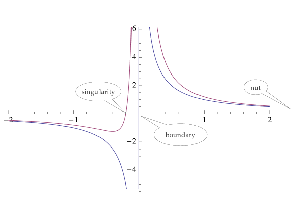
Figure 1: Generic solution $\Omega^{1}=\Omega^{2}<\Omega^{3}$.

The case where $\Omega^{1}\neq\Omega^{2}\neq\Omega^{3}$ is the most interesting in the present context since it involves quasimodular forms. The real Halphen solution (see Eq. (4.21) with $z=iT$ or $q=\exp-2\pi T$)) reads:

$$\begin{cases}\Omega^{1}_{\mathrm{H}}(T)=\frac{\pi}{6}\left(E_{2}-\vartheta_{2}^{4}-\vartheta_{3}^{4}\right)<0\\ \Omega^{2}_{\mathrm{H}}(T)=\frac{\pi}{6}\left(E_{2}+\vartheta_{3}^{4}+\vartheta_{4}^{4}\right)\\ \Omega^{3}_{\mathrm{H}}(T)=\frac{\pi}{6}\left(E_{2}+\vartheta_{2}^{4}-\vartheta_{4}^{4}\right)<\Omega^{2}_{\mathrm{H}}.\end{cases}$$ (5.8)

It is defined for $T>0$ with a pole at $T=0$:

$$\Omega^{1}_{\mathrm{H}}\approx-\frac{\pi}{2T^{2}},\quad\Omega^{2,3}_{\mathrm{H}}\approx\frac{1}{T}.$$ (5.9)

Around this pole, the behaviour of the metric is

$$\mathrm{d}s^{2}\approx-\left(\mathrm{d}\tau^{2}+\tau^{2}\left(\left(\sigma^{3}\right)^{2}+\left(\sigma^{2}\right)^{2}\right)+\frac{2}{\pi}\left(\sigma^{1}\right)^{2}\right),$$ (5.10)

and we recover a Taubian infinity ($S^{1}$ fiber over $\mathbb{R}^{3}$). The large-$T$ behaviour is exponential towards a constant

$$\Omega^{1,3}_{\mathrm{H}}\approx\mp 4\pi\exp{-\pi T},\quad\Omega^{2}_{\mathrm{H}}\approx\nicefrac{{\pi}}{{2}}+4\pi\exp{-2\pi T}$$ (5.11)

with

$$\mathrm{d}s^{2}\approx-\left(\mathrm{d}\tau^{2}+\frac{\pi}{2}\left(\left(\sigma^{1}\right)^{2}+\left(\sigma^{3}\right)^{2}\right)+4\tau^{2}\left(\sigma^{2}\right)^{2}\right).$$ (5.12)

This is precisely a bolt as in Eq. (5.2) with $n=4,\zeta=\sqrt{\nicefrac{{\pi}}{{2}}}$ and permutation of principal directions 2 and 3. All this is depicted in Fig. 2.

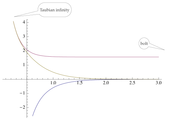
Figure 2: Halphen original solution ($\Omega^{1}_{\mathrm{H}}<0<\Omega^{3}_{\mathrm{H}}<\Omega^{2}_{\mathrm{H}}$).

As already quoted, the self-dual vacuum geometry corresponding to Halphen’s original solution is the Atiyah–Hitchin gravitational instanton [15]. Using modular transformations (4.9), one constructs all other real solutions with strict $SU(2)$ isometry (i.e. with all $\Omega^{i}$ different):

$$\Omega^{i}(T)=\frac{1}{\left(CT+D\right)^{2}}\Omega^{i}_{\mathrm{H}}\left(\frac{AT+B}{CT+D}\right)+\frac{C}{CT+D}.$$ (5.13)

Are those well behaved?

The answer is no because a root of one $\Omega$ always appears between the Taubian infinity and the bolt. This root is a curvature singularity, which spoils the regularity of the solution. In order to elaborate on that, we first observe that in Eq. (5.13), $\frac{AT+B}{CT+D}$ must be positive, as real $\Omega^{i}_{\mathrm{H}}$ are only defined for positive argument. Assume for concreteness that

$$\lim_{T\to\infty}\frac{AT+B}{CT+D}=\frac{A}{C}>0.$$ (5.14)

On the one hand, at large $T$

$$\Omega^{i}=\frac{1}{T}+\mathrm{O}\left(\nicefrac{{1}}{{T^{2}}}\right),$$ (5.15)

and trading $T$ for the local proper time one finds a nut (see (5.3)). On the other hand, the values $T_{\infty}=-\nicefrac{{D}}{{C}}<T_{0}=-\nicefrac{{B}}{{A}}$ correspond to two poles, and $\Omega^{i}(T)$ are defined for $T<T_{\infty}$ or $T_{0}<T$ with reflected behaviour. For $T_{0}\lessapprox T$

$$\Omega^{1}\approx-\frac{\pi}{2A^{2}}\frac{1}{\left(T-T_{0}\right)^{2}},\quad\Omega^{2,3}\approx\frac{1}{T-T_{0}}$$ (5.16)

(note the sign flip in $\Omega^{1}$) and

$$-\mathrm{d}s^{2}\approx\mathrm{d}\tau^{2}+\tau^{2}\left(\left(\sigma^{2}\right)^{2}+\left(\sigma^{3}\right)^{2}\right)+\frac{2A^{2}}{\pi}\left(\sigma^{1}\right)^{2}.$$ (5.17)

Therefore $T=T_{0}$ is a Taubian infinity ($S^{1}$ fiber over $\mathbb{R}^{3}$), and as $T$ moves from $T=T_{0}$ to $T\to+\infty$ one moves from the Taubian infinity (“boundary”) to a nut. A similar conclusion is reached when scanning $T$ from $T_{\infty}$ to $-\infty$.

The problem arises because there is always a value $T_{\ast}$ such that $T_{0}<T_{\ast}<\infty$ with $\Omega^{1}_{\ast}=0<\Omega^{3}_{\ast}<\Omega^{2}_{\ast}$ (see Fig. 3). This unavoidable root is a genuine curvature singularity of the metric. Because of this, no anisotropic solution of the Darboux–Halphen system other than the original one ((4.21) or (5.8)) provides a well-behaved Bianchi IX gravitational instanton.

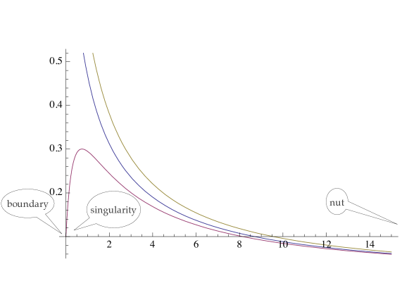
Figure 3: Generic solution for $T_{0}<T$ and $0<\Omega^{1}<\Omega^{3}<\Omega^{2}$.

5.3 A parenthesis on Ricci flows

Ricci flows describe the evolution of a metric on a manifold, governed by the following first-order equation:

$$\frac{\partial g_{ij}}{\partial t}=-R_{ij},$$ (5.18)

where $R_{ij}$ stands for the Ricci tensor of the Levi–Civita connection associated with $g_{ij}$ (see e.g. [55]). It was introduced by Hamilton in 1981 [56] in order to gain insight into the geometrization conjecture of Thurston (see e.g. [57]), a generalization of Poincaré’s 1904 conjecture for three-manifolds, finally demonstrated by Perel’man in 2003 [58]. Ricci flows are also important in modern physics as they describe the renormalization group evolution in two-dimensional sigma-models [59].

The case of homogeneous three-manifolds is important as it appears in the final stage of Thurston’s geometrization. Homogeneous three-manifolds include all 9 Bianchi groups plus 3 coset spaces, which are $H_{3}$, $H_{2}\times S^{1}$, $S^{2}\times S^{1}$ ($S^{n}$ and $H_{n}$ are spheres and hyperbolic spaces respectively) [60, 61]. The general asymptotic behaviour was studied in detail in [62]. A remarkable and already quoted result [45, 46, 47, 48] is the relationship between the parametric evolution of a metric

$$\mathrm{d}\tilde{s}^{2}=\sqrt{\frac{\Omega^{2}\Omega^{3}}{\Omega^{1}}}\left(\sigma^{1}\right)^{2}+\sqrt{\frac{\Omega^{3}\Omega^{1}}{\Omega^{2}}}\left(\sigma^{2}\right)^{2}+\sqrt{\frac{\Omega^{1}\Omega^{2}}{\Omega^{3}}}\left(\sigma^{3}\right)^{2}$$ (5.19)

on $\mathcal{M}_{3}$ of Bianchi type, and the time evolution inside a self-dual gravitational instanton on $\mathcal{M}_{4}=\mathbb{R}\times\mathcal{M}_{3}$ as given in (3.6): the equations are the same ($t$ in (5.18) and $T$ in (3.6) are related as $\mathrm{d}t=\sqrt{\Omega^{1}\Omega^{2}\Omega^{3}}\mathrm{d}T$). Ricci flow on three-spheres is therefore governed by the Darboux–Halphen equations (3.14).

Solutions of the Darboux–Halphen system describe Ricci-flow evolution if $\forall i\ \Omega^{i}(T)>0$, assuming that this holds at some initial time $T_{0}$. It is straightforward to see that this is always guaranteed. Indeed, it is true when at least two $\Omega$s are equal, as one can see directly from the algebraic solutions (5.4) and (5.5). More generally, suppose that $0<\Omega^{1}_{0}<\Omega^{2}_{0}<\Omega^{3}_{0}$ (the subscript refers to the initial time $T_{0}$) and that $\Omega_{1}$ has reached at time $T_{1}$ the value $\Omega_{1}^{1}=0$, while $\Omega^{2}_{1},\Omega^{3}_{1}>0$. From Eqs. (3.14) we conclude that at time $T_{1}$, $\dot{\Omega}_{2}^{1}=\dot{\Omega}_{3}^{1}=-\Omega_{2}^{1}\,\Omega_{3}^{1}<0$ and $\dot{\Omega}_{1}^{1}=\Omega_{2}^{1}\,\Omega_{3}^{1}>0$. This latter inequality implies that $\Omega_{1}$ vanishes at $T_{1}$ while it is increasing, passing therefore from negative to positive values. This could only happen if $\Omega^{1}_{0}$ were negative, which contradicts the original assumption. However, if indeed $\Omega^{1}_{0}<0$ and $\Omega^{2}_{0},\Omega^{3}_{0}>0$, there is a time $T_{1}$ where $\Omega^{1}$ becomes positive and remains positive together with $\Omega^{2}$ and $\Omega^{3}$ until they reach the asymptotic region.

Solutions (5.4) and (5.5) show that the asymptotic behaviour of $\Omega$s is clearly $\nicefrac{{1}}{{T}}$, when at least two $\Omega$s are equal. In the more general case, the large-$T$ behaviour is readily obtained thanks to the quasimodular properties of the solutions (see footnote 6):

$$\Omega^{1,2,3}(T)=-\frac{1}{T^{2}}\Omega^{2,1,3}\left(\frac{1}{T}\right)+\frac{1}{T}.$$ (5.20)

Therefore, for finite and positive $\Omega^{i}_{0}\equiv\Omega^{i}(0)$,

$$\Omega^{i}=\frac{1}{T}+\mathrm{subleading\ at\ large}\ T,$$ (5.21)

as one observes in Fig. 4. Note that this does not hold for the solution (5.8) because for the latter $T=0$ is a pole and $\Omega^{i}_{0}\equiv\Omega^{i}(0)$ is neither finite, nor positive for all $i$. The behaviour at large $T$ is not $\nicefrac{{1}}{{T}}$, but exponential (see Eq. (5.11) and Fig. 2).

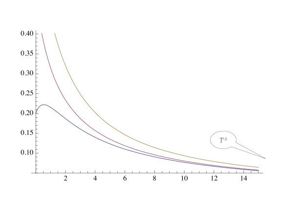
Figure 4: Generic behaviour for $0<\Omega^{1}_{0}<\Omega^{2}_{0}<\Omega^{3}_{0}$.

As a consequence of the generic behaviour (5.21) of $\Omega$s for positive and finite initial conditions, the late-time geometry on the $S^{3}$ under the Ricci flow is

$$\mathrm{d}s^{2}\approx\frac{1}{\sqrt{T}}\left(\left(\sigma^{1}\right)^{2}+\left(\sigma^{2}\right)^{2}+\left(\sigma^{3}\right)^{2}\right).$$ (5.22)

This is an isotropic (round) three-sphere of shrinking radius. It is worth stressing that this universal behaviour is specifically due to the quasimodular properties of the solution, reflected in the non-covariant $\nicefrac{{1}}{{T}}$ term of (5.20).

6 Bianchi IX foliations and conformal self-duality

So far, we have considered self-dual solutions of Einstein’s equations. These satisfy Eqs. (2.23) and are Ricci flat. Solutions of the Darboux–Halphen system involving quasimodular forms are relevant in particular when Bianchi IX foliations are considered. The Lagrange and Darboux–Halphen systems, and more general modular and quasimodular forms emerge, however, in set ups where no self-duality and/or Bianchi IX foliation is assumed. Einstein conformally (anti-)self-dual spaces i.e. quaternionic spaces turn out to exhibit such interesting relationships.

Conformally self-dual Einstein spaces satisfy (see Eqs. (2.29))

$$\widehat{\mathcal{W}}^{-}_{i}=0.$$ (6.1)

This two–form is defined in (2.28) as the anti-self-dual part of the on-shell Weyl tensor (2.26). The latter includes a cosmological constant $\Lambda$ and (6.1) implies that this space is Einstein ($R_{ab}=\Lambda g_{ab}$) on top of being conformally self-dual ($W^{-}=0$).

6.1 Conformally self-dual Bianchi IX foliations

Assuming the four-dimensional space be a foliation $\mathcal{M}_{4}=\mathbb{R}\times\mathcal{M}_{3}$ with $\mathcal{M}_{3}$ a general homogeneous three-sphere invariant under $SU(2)$ isometry, we can in general endow it with a metric (3.6). The Levi–Civita connection one–forms of the latter are given in (3.9) and (3.10)). Conformal self-duality condition (6.1) does not require the flatness of the anti-self-dual component of the connection $A_{i}$ as in (3.11). Hence, no first integral like (3.12) is available.

In order to take advantage of the conformal self-duality condition (6.1) and reach first-order differential equations as in the case of pure self-duality, we can parameterize the connection $A_{i}$ and $\Sigma_{i}$ and demand that (6.1) be satisfied. This is usually done by setting both $A_{i}$ and $\Sigma_{i}$ proportional to $\sigma^{i}$, as in (3.12), with a $T$-dependent coefficient though (see e.g. [63]):

$$\Sigma_{i} = -\frac{B_{i}}{2\Omega^{i}}\sigma^{i},$$ (6.2)

$$A_{i} = \frac{\Delta_{i}}{2\Omega^{i}}\sigma^{i}.$$ (6.3)

Using Eqs. (3.9) and (3.10), one obtains a relationship between $\left\{\dot{\Omega}^{i}\right\}$ and $\left\{B_{i},\Delta_{i}\right\}$:

$$\dot{\Omega}^{i}={\Omega^{j}\Omega^{k}}-\Omega^{i}\left(\Delta_{j}+\Delta_{k}\right)=-{\Omega^{j}\Omega^{k}}+\Omega^{i}\left(B_{j}+B_{k}\right).$$ (6.4)

Furthermore, Eqs. (2.27) and (2.28) lead to the following expressions for the on-shell Weyl tensor:

$$\widehat{\mathcal{W}}^{+}_{i} = -\left\{\frac{1}{4\Omega^{1}\Omega^{2}\Omega^{3}}\left(\dot{B}_{i}+B_{j}B_{k}-B_{i}\left(B_{j}+B_{k}\right)\right)+\frac{\Lambda}{6}\right\}\phi^{i}$$ (6.5)

$$-\left\{\frac{1}{4\Omega^{1}\Omega^{2}\Omega^{3}}\left(\dot{B}_{i}-B_{j}B_{k}-B_{i}\left(B_{j}+B_{k}\right)\right)+\frac{B_{i}}{2\left(\Omega^{i}\right)^{2}}\right\}\chi^{i},$$

$$\widehat{\mathcal{W}}^{-}_{i} = \left\{\frac{1}{4\Omega^{1}\Omega^{2}\Omega^{3}}\left(\dot{\Delta}_{i}+\Delta_{j}\Delta_{k}+\Delta_{i}\left(\Delta_{j}+\Delta_{k}\right)\right)-\frac{\Delta_{i}}{2\left(\Omega^{i}\right)^{2}}\right\}\phi^{i}$$ (6.6)

$$+\left\{\frac{1}{4\Omega^{1}\Omega^{2}\Omega^{3}}\left(\dot{\Delta}_{i}-\Delta_{j}\Delta_{k}+\Delta_{i}\left(\Delta_{j}+\Delta_{k}\right)\right)-\frac{\Lambda}{6}\right\}\chi^{i}.$$

The additional (with respect to (6.4)) first-order equations for $\left\{B_{i}\right\}$ or $\left\{\Delta_{i}\right\}$ are obtained by imposing on-shell conformal self-duality. The canonical method for that is to demand that both coefficients of $\phi^{i}$ and $\chi^{i}$ in (6.6) vanish. This guarantees (see (2.27)) a conformally self-dual, Einstein manifold with scalar curvature $R=4\Lambda$, in other words a quaternionic space.

Solving the system of equations obtained for conformally self-dual, Einstein manifolds depends drastically on whether or not the isometry is strictly $SU(2)$, i.e. the leaves of the Bianchi IX foliation are anisotropic, triaxial spheres. When the isometry is extended to $SU(2)\times U(1)$ (two equal $\Omega$s), the equations are algebraically integrable (as in the Darboux–Halphen system (3.14)) and no relationship appears with modular or quasimodular forms. This leads to a variety of well known biaxial solutions (see [16, 17, 63] as well as [64] for a detailed presentation of the resolution) such as (anti-)de Sitter–Taub–NUT, (anti-)de Sitter–Eguchi–Hanson, (pseudo-)Fubini–Study – $\mathbb{C}P_{2}$, Pedersen (the parentheses correspond to negative $\Lambda$) …When all $\Omega$s are equal, the leaves are round, uniaxial three-spheres, and the only four-geometries are the symmetric $S^{4}$ or $H_{4}$ (depending again on the sign of $\Lambda$).

Although straightforward, the above approach leads for the triaxial case to equations which are not known to be integrable. Hence, their resolution is not systematic and general. An alternative strategy has been proposed by Tod and Hitchin [65, 66], based on twistor spaces and isomonodromic deformations (see also [67, 68]). In a first step, one sets $\Lambda$ to zero in (6.6) and demands the coefficient of $\chi^{i}$ to vanish. This is equivalent to demanding conformal self-duality and zero scalar curvature ($W^{-}=s=0$) without setting $C^{-}_{ij}$ to zero. Thus, the space is not Einstein and has zero scalar curvature. The final step is to perform a conformal transformation, which allows to restore a non-vanishing scalar curvature, while simultaneously setting $C^{-}_{ij}=0$. One thus obtains a quaternionic space.

Explaining the details of this procedure is beyond our present scope, and we will therefore limit our presentation to the issues involving modular forms, which stem out of conditions $W^{-}=s=0$. These are imposed by demanding that the coefficient of $\chi^{i}$ vanishes in (6.6) and setting $\Lambda=0$:

$$\mathrm{I}\quad\begin{cases}\dot{\Delta}_{1}=\Delta_{2}\Delta_{3}-\Delta_{1}\left(\Delta_{2}+\Delta_{3}\right)\\ \dot{\Delta}_{2}=\Delta_{3}\Delta_{1}-\Delta_{2}\left(\Delta_{3}+\Delta_{1}\right)\\ \dot{\Delta}_{3}=\Delta_{1}\Delta_{2}-\Delta_{3}\left(\Delta_{1}+\Delta_{2}\right).\end{cases}$$ (6.7)

They are supplemented with Eqs. (6.4), which read for $\left\{\Delta_{i}\right\}$:

$$\mathrm{II}\quad\begin{cases}\dot{\Omega}^{1}=\Omega^{2}\Omega^{3}-\Omega^{1}\left(\Delta_{2}+\Delta_{3}\right)\\ \dot{\Omega}^{2}=\Omega^{3}\Omega^{1}-\Omega^{2}\left(\Delta_{3}+\Delta_{1}\right)\\ \dot{\Omega}^{3}=\Omega^{1}\Omega^{2}-\Omega^{3}\left(\Delta_{1}+\Delta_{2}\right).\end{cases}$$ (6.8)

Before pursuing the present investigation any further, it is worth making contact with the results of Sec. 3.2 on genuine self-duality equations. Assuming the system I and II satisfied i.e. $W^{-}=s=0$, $\mathcal{A}_{i}$ (Eq. (2.21)) reads:

$$\mathcal{A}_{i}=\frac{1}{2}C^{-}_{ij}\phi^{j}=\frac{1}{2\Omega^{i}}\left(\frac{\Delta_{j}\Delta_{k}}{\Omega^{j}\Omega^{k}}-\frac{\Delta_{i}}{\Omega^{i}}\right)\phi^{i}.$$ (6.9)

Purely self-dual Einstein vacuum spaces are obtained by demanding $C^{-}_{ij}=0$ (i.e. $R_{ab}=0$ since the scalar curvature vanishes). This leads to the two known possibilities for Bianchi IX vacuum self-dual Einstein geometries met in Sec. 3.2, and satisfying either one of the following systems:

• Lagrange (3.13) for $\Delta_{i}=0$,

• Darboux–Halphen (3.14) for $\Delta_{i}=\Omega^{i}$.

6.2 Solving I & II with Painlevé VI

Systems I and II (Eqs. (6.7) and (6.8)) describing general conformally self-dual Bianchi IX foliations with vanishing scalar curvature ($W^{-}=s=0$) were studied e.g. in [69, 70] prior to their uplift to quaternionic spaces. Further developments in relation with modular properties can be found in [71, 72].

As usual it is convenient to move to the complex plane, introduce $\omega^{\ell}(z)$ and $\delta_{\ell}(z)$ and trade the dot for a prime as derivative with respect to $z$ in (6.7) and (6.8). Real solutions are recovered as previously: $\Omega^{\ell}(T)=i\omega^{\ell}(iT)$ and $\Delta_{\ell}(T)=i\delta_{\ell}(iT)$.

The system I is that of Darboux–Halphen for $\delta_{i}(z)$ (see (3.14)). Given a solution $\delta_{i}(z)$ one can solve the system II for $\omega^{i}(z)$. Furthermore, the $SL(2,\mathbb{C})$ solution-generating technique described in (4.2) can be generalized in the present case: given a solution $\delta_{i}(z)$ and $\omega^{i}(z)$,

$$\tilde{\delta}_{i}(z)=\frac{1}{\left(cz+d\right)^{2}}\delta_{i}\left(\frac{az+b}{cz+d}\right)+\frac{c}{cz+d}$$ (6.10)

and

$$\tilde{\omega}^{i}(z)=\frac{1}{\left(cz+d\right)^{2}}\omega^{i}\left(\frac{az+b}{cz+d}\right)$$ (6.11)

provide another solution if $\left(\begin{smallmatrix}a&b\\ c&d\end{smallmatrix}\right)\in SL(2,\mathbb{C})$.

Assuming $\delta_{1}\neq\delta_{2}\neq\delta_{3}$ i.e. the triaxial situation (implying automatically $\omega^{1}\neq\omega^{2}\neq\omega^{3}$), we can readily obtain the general solution of the system I as in (4.7),

$$\delta_{i}(z)=-\frac{1}{2}\frac{\mathrm{d}}{\mathrm{d}z}\log\mathcal{E}^{i}(z),$$ (6.12)

with $\mathcal{E}^{i}(z)$ a triplet of weight-two modular forms of $\Gamma(2)\subset SL(2,\mathbb{Z})$. These can be expressed as in (4.12), where $\lambda$ is a solution of Schwartz’s equation (4.11). Define now a new set of functions $w_{i}(z)$ as

$$w_{i}=\frac{\omega^{i}}{\sqrt{\mathcal{E}^{j}\mathcal{E}^{k}}}$$ (6.13)

($i,j,k$ cyclic permutation of $1,2,3$), and insert the solutions (6.12) in system II (6.8). The latter becomes

$$\frac{\mathrm{d}w_{1}}{\mathrm{d}\lambda}=\frac{w_{2}w_{3}}{\lambda},\quad\frac{\mathrm{d}w_{2}}{\mathrm{d}\lambda}=\frac{w_{3}w_{1}}{\lambda-1},\quad\frac{\mathrm{d}w_{3}}{\mathrm{d}\lambda}=\frac{w_{1}w_{2}}{\lambda(\lambda-1)}.$$ (6.14)

Notice the first integral $w_{1}^{2}-w_{2}^{2}+w_{3}^{2}$. Even though the value of this integral is arbitrary, the uplift of the corresponding conformally self-dual geometry with zero scalar curvature to an Einstein manifold is possble only if the constant is $\nicefrac{{1}}{{4}}$ (see [65, 66]).

The system of equations (6.14) can be solved in full generality with $w_{i}$ expressed in terms of solutions $y(\lambda)$ of Painlevé VI equation [73] (see also [74] for a more general overview):

$$w_{1}^{2} = \frac{(y-\lambda)y^{2}(y-1)}{\lambda}\left(v-\frac{1}{2(y-1)}\right)\left(v-\frac{1}{2(y-\lambda)}\right),$$ (6.15)

$$w_{2}^{2} = \frac{(y-\lambda)y(y-1)^{2}}{\lambda-1},\left(v-\frac{1}{2y}\right)\left(v-\frac{1}{2(y-\lambda)}\right)$$ (6.16)

$$w_{3}^{2} = \frac{(y-\lambda)^{2}y(y-1)}{\lambda(\lambda-1)}\left(v-\frac{1}{2y}\right)\left(v-\frac{1}{2(y-1)}\right).$$ (6.17)

Here,

$$v=\frac{\lambda(\lambda-1)y^{\prime}}{2y(y-1)(y-\lambda)}+\frac{1}{4y}+\frac{1}{4(y-1)}-\frac{1}{4(y-\lambda)}$$ (6.18)

and $y$ is a solution of Painlevé VI equation ($f^{\prime}=\nicefrac{{\mathrm{d}f}}{{\mathrm{d}\lambda}}$):

$$y^{\prime\prime} = \frac{1}{2}\left(\frac{1}{y}+\frac{1}{y-1}+\frac{1}{y-\lambda}\right)(y^{\prime})^{2}-\left(\frac{1}{\lambda}+\frac{1}{\lambda-1}+\frac{1}{y-\lambda}\right)y^{\prime}$$ (6.19)

$$+\frac{(y-\lambda)y(y-1)^{2}}{8\lambda^{2}(\lambda-1)^{2}}\left({1}-\frac{\lambda}{y^{2}}+\frac{\lambda-1}{(y-1)^{1}}-\frac{3\lambda(\lambda-1)}{(y-\lambda)^{2}}\right).$$

6.3 Back to quasimodular forms

We will for concreteness concentrate on the original solution of system I, the Halphen solution corresponding to $\lambda_{\mathrm{H}}=\nicefrac{{\vartheta_{2}^{4}}}{{\vartheta_{3}^{4}}}$. This is sufficient as any other can be generated by $SL(2,\mathbb{C})$ transformations. Equations (6.14) (system II) read now

$$w_{1}^{\prime}=i\pi\vartheta_{4}^{4}w_{2}w_{3},\quad w_{2}^{\prime}=-i\pi\vartheta_{2}^{4}w_{3}w_{1},\quad w_{1}^{\prime}=-i\pi\vartheta_{3}^{4}w_{2}w_{3}.$$ (6.20)

In this form, the system can be solved in terms of Jacobi theta functions with characteristics [72], as an alternative to the solution (6.15)–(6.17). This makes it relevant in the present framework.

The solution with $w_{1}^{2}-w_{2}^{2}+w_{3}^{2}=\nicefrac{{1}}{{4}}$ – required for the subsequent promotion to quaternionic geometries – read:

$$w_{1}(z) = \frac{1}{2\pi\vartheta_{2}(0|z)\vartheta_{3}(0|z)}\frac{\partial_{v}\vartheta{a+1\atopwithdelims[ ]b}(0|z)}{\vartheta{a\atopwithdelims[ ]b}(0|z)},$$ (6.21)

$$w_{2}(z) = \frac{\mathrm{e}^{-i\pi\nicefrac{{a}}{{2}}}}{2\pi\vartheta_{3}(0|z)\vartheta_{4}(0|z)}\frac{\partial_{v}\vartheta{a\atopwithdelims[ ]b+1}(0|z)}{\vartheta{a\atopwithdelims[ ]b}(0|z)},$$ (6.22)

$$w_{3}(z) = \frac{-\mathrm{e}^{-i\pi\nicefrac{{a}}{{2}}}}{2\pi\vartheta_{2}(0|z)\vartheta_{4}(0|z)}\frac{\partial_{v}\vartheta{a+1\atopwithdelims[ ]b+1}(0|z)}{\vartheta{a\atopwithdelims[ ]b}(0|z)}.$$ (6.23)

Here $a,b\in\mathbb{C}$ are moduli, mapped under the $SL(2,\mathbb{C})$ transformations (6.10) and (6.11) to other complex numbers. If $a,b$ are integers and the transformation is in $SL(2,\mathbb{Z})$, the solution is left invariant, up to permutation of the three components.

It would be interesting to present the geometrical structure of the conformally self-dual zero-curvature spaces obtained with the solutions at hand, following the general procedure used in Sec. 5.2. This would definitely bring us far from the original goal. The interested reader can find useful information in the already quoted literature, both for these spaces and for their quaternionic uplift. Note in that respect that even though many families of solutions exist (here in the triaxial case, or more generally for biaxial three-sphere foliations), very few are singularity-free among which, the Fubini–Study or the Pedersen instanton ($SU(2)\times U(1)$ isometry), or the Hitchin–Tod solution (strict $SU(2)$ symmetry).

As a final remark, let us mention that (6.21), (6.22), (6.23) also capture the self-dual Ricci flat solutions discussed in Sec. 3 and given in Eqs. (4.21) i.e. the Atiyah–Hitchin gravitational instanton. They correspond to the choice $a=b=1\ \mathrm{mod}\ 2$, that must be implemented with care: consider $a=1+2\epsilon,b=1+2z_{0}\epsilon$ and take the limit $\epsilon\to 0$. One finds (a useful identity for this computation is given in (A.5):

$$w_{1} = -\frac{1}{\pi\vartheta_{2}^{2}\vartheta_{3}^{2}}\left(\frac{i}{z+z_{0}}-\frac{\pi}{6}\left(E_{2}-\vartheta_{2}^{4}-\vartheta_{3}^{4}\right)\right),$$ (6.24)

$$w_{2} = -\frac{i}{\pi\vartheta_{3}^{2}\vartheta_{4}^{2}}\left(\frac{i}{z+z_{0}}-\frac{\pi}{6}\left(E_{2}+\vartheta_{3}^{4}+\vartheta_{4}^{4}\right)\right),$$ (6.25)

$$w_{3} = -\frac{i}{\pi\vartheta_{2}^{2}\vartheta_{4}^{2}}\left(\frac{i}{z+z_{0}}-\frac{\pi}{6}\left(E_{2}+\vartheta_{2}^{4}-\vartheta_{4}^{4}\right)\right).$$ (6.26)

A modulus $z_{0}$ is left in the solution; under $SL(2,\mathbb{Z})$ it transforms as

$$z_{0}\to\frac{dz_{0}+b}{cz_{0}+a}.$$ (6.27)

For finite $z_{0}$ the corresponding metric is Weyl-self-dual with zero scalar curvature The $z_{0}\to i\infty$ limit corresponds to the Ricci-flat, Atiyah–Hitchin instanton (Riemann-self-dual).

6.4 Beyond Bianchi IX foliations

We would like to close our overview on conformally self-dual geometries with another family of quaternionic solutions, related to modular forms but not of the type $\mathcal{M}_{4}=\mathbb{R}\times\mathcal{M}_{3}$ with homogeneous $\mathcal{M}_{3}$. Indeed, self-duality (Eq. (2.23)) or conformal self-duality (Eqs. (2.24) and (2.25)) can be demanded outside ot the framework of foliations.

On can indeed assume an ansatz for the metric of the Gibbons–Hawking type [14]:

$$\mathrm{d}s^{2}=\Phi^{-1}\left(\mathrm{d}\tau+\varpi_{i}\mathrm{d}x^{i}\right)^{2}+\Phi\delta_{ij}\mathrm{d}x^{i}\mathrm{d}x^{j}.$$ (6.28)

Here $\Phi$ and $\varpi_{i}$ depend on $\mathbf{x}$ only, and thus $\partial_{\tau}$ is Killing. With this ansatz more general self-dual solutions are obtained with $U(1),U(1)\times U(1)$ or $U(1)\times\mathrm{Bianchi}$ isometry. Determining quaternionic spaces, i.e. conformally self-dual and Einstein, is however far more difficult. It is a real tour de force to find the most general quaternionic solution with $U(1)\times U(1)$ isometry and this was achieved by Calderbank and Pedersen in [21], following the original method of Lebrun [68]. This will be our last example, where a new kind of modular forms emerge.

In coordinates $\{\rho,\eta,\theta,\psi\}$ with frame

$$\alpha=\sqrt{\rho}\mathrm{d}\rho,\quad\beta=\frac{\mathrm{d}\psi+\eta\mathrm{d}\theta}{\sqrt{\rho}},\quad\gamma=\mathrm{d}\rho,\quad\delta=\mathrm{d}\eta,$$ (6.29)

The metric reads:

$$\mathrm{d}s^{2} = \frac{4\rho^{2}\left(F^{2}_{\rho}+F^{2}_{\eta}\right)-F^{2}}{4F^{2}\rho^{2}}\left(\gamma^{2}+\delta^{2}\right)$$ (6.30)

$$+\frac{\left[\left(F-2\rho F_{\rho}\right)\alpha-2\rho F_{\eta}\beta\right]^{2}+\left[\left(F+2\rho F_{\rho}\right)\beta-2\rho F_{\eta}\alpha\right]^{2}}{F^{2}\left[4\rho^{2}\left(F^{2}_{\rho}+F^{2}_{\eta}\right)-F^{2}\right]}.$$

Here $F_{\rho}=\partial_{\rho}F$ and $F_{\eta}=\partial_{\eta}F$, where $F(\rho,\eta)$ is a solution of

$$\rho^{2}\left(\partial^{2}_{\rho}+\partial^{2}_{\eta}\right)F=\tfrac{3}{4}F.$$ (6.31)

The metric (6.30) has generically two Killing vectors, $\partial_{\theta},\partial_{\psi}$ and $F(\rho,\eta)$ is a harmonic function on $H_{2}$ with eigenvalue $\nicefrac{{3}}{{4}}$. Indeed, the metric on the hyperbolic plane is

$$\mathrm{d}s_{H_{2}}^{2}=\frac{\mathrm{d}\rho^{2}+\mathrm{d}\eta^{2}}{\rho^{2}}$$ (6.32)

and Eq. (6.31) can be recast as

$$\triangle_{H_{2}}F=\tfrac{3}{4}F.$$ (6.33)

Solving (6.33) leads inevitably to modular forms of $\tau=\eta+i\rho$, even though algebraic solutions are also available.

Let us mention for example

$$F=\sqrt{\rho+\frac{\eta^{2}}{\rho}},$$ (6.34)

which leads to a metric on $\mathbb{C}P_{2}$ with $U(1)\times SU(2)$ isometry [18], or

$$F=\frac{\rho^{2}-\rho_{0}^{2}}{2\sqrt{\rho}}$$ (6.35)

with $U(1)\times\mathrm{Heisenberg}$ symmetry [75]. Solutions for $F(\rho,\eta)$ with strict $U(1)\times U(1)$ isometry open Pandora’s box for non-holomorphic Eisenstein series such as (see (A.9))

$$F=E_{\nicefrac{{3}}{{2}}}(\tau,\bar{\tau}),$$ (6.36)

which has a further discrete residual symmetry $SL(2,\mathbb{Z})\subset SL(2,\mathbb{R})$. These will be discussed in Sec. 7 and we refer to the appendix for some precise definitions. Very little is known at present on the geometrical properties of the corresponding quaternionic spaces, or on the fields of application these spaces could find in physics. In string theory, they are known to describe the moduli space of hypermultiplets in compactifications on Calabi–Yau threefolds [76]. The relevance of the Calderbank and Pedersen metrics in this context was recognized in [77]. For further considerations on the role of modular and quasimodular foms as string instantonic contributions to the moduli spaces of these compactifications, we refer to [78, 79, 80, 81, 82, 83] and in particular to the recent review [84].

7 Beyond the world of Eisenstein series

To end up this review we would like to elaborate on some connections between quantum field theory and modular forms. This originates from the specific structure of the perturbative expansions in string and field theory, and calls for develping more general modular functions than the non-holomorphic Eisenstein series discussed earlier in these notes.

7.1 The starting point: perturbation theory

Perturbative expansions in quantum field theory are expressed as sums of multidimensional integrals, obtained by applying Feynman rules or unitarity constraints. These integrals are plagued by various divergences that need to be regulated. It was remarked in [85, 86] that the coefficients of these divergences are given by multiple zeta values in four dimensions. Since this original work, it has become more and more important to further investigate the relationship between quantum field theory and the structure of multiple zeta values. This connection has fostered important mathematical results as in instance [87, 88], which have been reviewed in the recent Séminaire Bourbaki by Pierre Deligne [89].

The next observation is that the above mentioned field-theory Feynman integrals arise as certain limits of string-theory integrals defined on higher-genus Riemann surfaces. They are actually obtained from the boundary of the moduli of higher-genus punctured Riemann surfaces. This bridge to string theory sets a handle to the world of modular functions.

There are indeed two motivations for embedding the analysis into a string theory framework. The first is of physical nature: perturbative string theory is free of ultraviolet divergences, so it provides a well-defined prescription for regularizing field-theory divergences. In other words, string theory acts as a specific regularization from which we expect to learn more on the fundamental structure of the quantum field theories. The second motivation is directly related to the topic of this text: string theory is the ideal arena for exploring the number theoretic considerations of quantum field theory and their close connection with modular forms.

In the present notes we will focus on the case of the tree level and genus one, following the string analysis in [90, 22] and the mathematical analysis in [91]. We will explain in particular that (non-holomorphic) Eisenstein series are not enough for capturing all available information carried by the integrals under consideration. The presentation will be schematic, aiming at conveying a message rather that providing all technical details. For the latter, the interested reader is referred to the quoted literature.

Let us consider the following integral defined on the moduli space of the genus-$g$ Riemann surface with four marked points:

$$A^{(g)}(s,t,u)=\int_{\mathcal{M}_{g}}\mathrm{d}\mu\,\int_{\Sigma_{g}}\prod_{i=1}^{4}\mathrm{d}^{2}z_{i}\,\exp\left(\sum_{1\leq i<j\leq 4}2\alpha^{\prime}k_{i}\cdot k_{j}P(z_{i},z_{j})\right),$$ (7.1)

where $\mathcal{M}_{g}$ is the moduli space of the closed Riemann surface $\Sigma_{g}$ of genus $g$. There are four punctures whose positions $z_{i}$ are integrated over. We have introduced $k_{1}+k_{2}+k_{3}+k_{4}=0$ with $k_{i}\cdot k_{i}=0$ representing external massless momenta flowing into each puncture. We will also set the Mandelstam variables $s=2k_{1}\cdot k_{2}=2k_{3}\cdot k_{4}$, $t=2k_{1}\cdot k_{4}=2k_{2}\cdot k_{3}$ and $u=2k_{1}\cdot k_{3}=2k_{2}\cdot k_{4}$, obeying $s+t+u=0$ for the massless states at hand. The physical scale is the inverse tension of the string $\alpha^{\prime}$.

The propagator or Green’s function $P(z,w)$ is defined on this Riemann surface by

$$0 = \int_{\Sigma_{g}}\mathrm{d}^{2}z\,\sqrt{-g}\,P(z,w),$$ (7.2)

$$\partial_{z}\bar{\partial}_{\bar{z}}P(z,w) = 2\pi\delta^{(2)}(z)-{2\pi g_{z\bar{z}}\over\int_{\Sigma_{g}}\mathrm{d}^{2}z\sqrt{-g}},$$ (7.3)

$$\partial_{z}\bar{\partial}_{\bar{w}}P(z,w) = -2\pi\delta^{(2)}(z)+\pi\sum_{I=1}^{g}\omega_{I}(z)(\Im m\Omega)^{-1}_{IJ}\omega_{J}(w),$$ (7.4)

where the $\mathrm{d}s^{2}=g_{z\bar{z}}\mathrm{d}z\mathrm{d}\bar{z}$ is the metric on the Riemann, $\Omega$ the period matrix, and $\omega_{I}$ with $1\leq I\leq g$ the first Abelian differentials.

7.2 Genus zero: the Eisenstein series

At genus 0, i.e. for the Riemann sphere, the propagator is simply given by

$$P^{(0)}(z,w)=\log|z-w|^{2},$$ (7.5)

and the integral in (7.1) can be evaluated to give

$$A^{(0)}(s,t,u) = {1\over\alpha^{\prime 3}stu}\,{\Gamma\left(1+\alpha^{\prime}s\right)\Gamma\left(1+\alpha^{\prime}t\right)\Gamma\left(1+\alpha^{\prime}u\right)\over\Gamma\left(1-\alpha^{\prime}s\right)\Gamma\left(1-\alpha^{\prime}t\right)\Gamma\left(1-\alpha^{\prime}u\right)}$$ (7.6)

$$= {1\over\alpha^{\prime 3}stu}\,\exp\left(-\sum_{n=1}^{\infty}{2\zeta(2n+1)\over 2n+1}\left[(\alpha^{\prime}s)^{n}+(\alpha^{\prime}t)^{n}+(\alpha^{\prime}u)^{n}\right]\right).$$

The masses of string theory excitations are integer, quantized in units of $\nicefrac{{1}}{{\alpha^{\prime}}}$. It is therefore expected that the $\alpha^{\prime}$ expansion of the string amplitude in (7.6) is given by multiple sums over the integers, but it is remarkable that this expansion involves only odd zeta values of depth one. For $\alpha^{\prime}\ll 1$ a series expansion representation reads:

$$A^{(0)}(s,t,u)=\sum_{q\geq-1,p\geq 0}c_{(p,q)}\,\sigma_{2}^{p}\sigma_{3}^{q},$$ (7.7)

where we have introduced $\sigma_{2}=(\alpha^{\prime}s)^{2}+(\alpha^{\prime}t)^{2}+(\alpha^{\prime}u)^{2}$ and $\sigma_{3}=3\alpha^{\prime 3}stu$. Since $\sigma_{1}=(\alpha^{\prime}s)+(\alpha^{\prime}t)+(\alpha^{\prime}u)=0$, we immediately see that all $\sigma_{n}=(\alpha^{\prime}s)^{n}+(\alpha^{\prime}t)^{n}+(\alpha^{\prime}u)^{n}$ with $n\geq 2$ are given by [90]

$${\sigma_{n}\over n}=\sum_{2p+3q=n}{(p+q-1)!\over p!q!}\,\left(\sigma_{2}\over 2\right)^{p}\left(\sigma_{3}\over 3\right)^{q}.$$ (7.8)

The coefficients $c_{(p,q)}$ are polynomial in odd zeta values of weight $2p+3q-3$. It is notable that at a given order $n=2p+3q-3$, the space of these coefficients has dimension $d_{n}=\left\lfloor(n+2)/2\right\rfloor-\left\lfloor(n+2)/3\right\rfloor$, which coincides with the dimension of the space of the holomorphic Eisenstein series of weight $n$ (see appendix). This hint calls for further investigation, and we would like to mention the recent work connecting the $\alpha^{\prime}$ expansion in (7.7) and the motivic multiplet zeta values [92].

One can expand the integrand of (7.7) and obtain each coefficient $c_{(p,q)}$ as a linear combination of the multiple integrals of the propagator $P^{(0)}(z_{i},z_{j})$ (given in (7.5)):

$$c_{n_{12},n_{13},n_{14},n_{23},n_{24},n_{34}}=\int_{S^{2}}\prod_{1\leq i<j\leq 4}\mathrm{d}^{2}z_{i}\,\prod_{1\leq i<j\leq 4}P^{(0)}(z_{i},z_{j})^{n_{ij}}.$$ (7.9)

The integrand of this expression is the product of the propagators connecting the punctures with multiplicities $n_{ij}$, $1\leq i<j\leq 4$, as depicted on Fig. 5.

Figure 5: Graph of a vacuum Feynman diagram on the Riemann surface $\Sigma_{g}$. The punctures are connected by $n_{ij}\geq 0$ links representing the number of two-dimensional propagators.

The contributions in (7.7) are the lowest-order to the full string-theory amplitude of the four-point (four punctures) processes described here.

In Eqs. (7.6)–(7.7), we encountered the zeta values

$$\zeta(s)=\sum_{n\geq 1}{1\over n^{s}}.$$ (7.10)

Extending the sum over the integers $n$ to a lattice like $\mathbf{p}=m+\tau n\in\Lambda^{(1)}=\mathbb{Z}+\tau\mathbb{Z}$, where $\tau\in\mathfrak{h}=\{z\in\mathbb{C},\Im m(z)\geq 0\}$, one gets the (non-holomorphic) Eisenstein series

$$\hat{E}_{s}(\tau,\bar{\tau})=\sum_{\mathbf{p}\in\mathbb{Z}+\tau\mathbb{Z}}{1\over|\mathbf{p}|^{2s}},$$ (7.11)

where $|\mathbf{p}|^{2}=(m+n\tau)(m+n\bar{\tau})$ is the natural Euclidean norm on the lattice $\Lambda^{(1)}$. This expression can be made modular-invariant in a trivial way by multiplying by $\Im m(\tau)^{s}$,

$$E_{s}(\tau,\bar{\tau})=\sum_{\mathbf{p}\in\mathbb{Z}+\tau\mathbb{Z}}{\Im m(\tau)^{s}\over|\mathbf{p}|^{2s}}.$$ (7.12)

This Eisenstein series is an eigenfunction of the hyperbolic Laplacian (6.31) with eigenvalue $s(s-1)$:

$$\triangle_{H_{2}}E_{s}(\tau,\bar{\tau})=s(s-1)\,E_{s}(\tau,\bar{\tau}).$$ (7.13)

The case $s=\nicefrac{{3}}{{2}}$ was discussed in Sec. 6.4, Eqs. (6.34)–(6.36), from a different physical perspective.

7.3 Genus one: beyond

At this stage of the exposition the reader may wonder how the above generalization of the zeta values (7.10) into modular forms (7.12) arises in string theory. We will sketch how this goes and show that new automorphic forms are actually needed, standing beyond the well known Eisenstein series. This requires going beyond the sphere (7.5)–(7.7).

At genus one, the Green’s function is given by

$$P^{(1)}(z,0)=-\frac{1}{4}\log\left|\vartheta_{1}(z|\tau)\over\vartheta_{1}^{\prime}(0|\tau)\right|^{2}+{\pi\Im m(z)^{2}\over 2\tau_{2}}.$$ (7.14)

The amplitude in (7.1) reads:

$$A^{(1)}(s,t,u)=\int_{\mathcal{F}}{\mathrm{d}^{2}\tau\over\tau_{2}^{2}}\int_{\mathcal{T}}\prod_{1\leq i<j\leq 4}{\mathrm{d}^{2}z_{i}\over\tau_{2}}\,\mathcal{W}^{(1)}\,\mathrm{e}^{-\sum_{1\leq i<j\leq 4}2\alpha^{\prime}k_{i}\cdot k_{j}\hat{P}^{(1)}(z_{i}-z_{j})},$$ (7.15)

where $\mathcal{F}=\left\{\tau;|\Re e(\tau)|\leq\frac{1}{2},\Im m(\tau)>0,\Re e(\tau)^{2}+\Im m(\tau)^{2}\geq 1\right\}$ is a fundamental domain for $SL(2,\mathbb{Z})$, and $\mathcal{T}=\left\{z;|\Re e(z)|\leq\frac{1}{2},0\leq\Im m(z)\leq\Im m(\tau)\right\}$.

No closed form for the integral in (7.15) is known, in particular because of the presence of non-analytic contributions in the complex $(s,t)$-plane. For a rigorous definition of this integral we refer to [93]. The expression for the genus-one propagator in (7.14) has an alternative representation:

$$P^{(1)}(z,0)={1\over 2\pi}\sum_{\mathbf{p}\in\mathbb{Z}+\tau\mathbb{Z}}\,{\tau_{2}\over|\mathbf{p}|^{2}}\,\mathrm{e}^{-\pi{\Im m(\bar{z}\mathbf{p})\over\tau_{2}}}+C(\tau,\bar{\tau}),$$ (7.16)

where $C(\tau,\bar{\tau})=\log|\sqrt{2\pi}\eta(\tau)|$ is a modular anomaly. Since the latter is $z$-independent, it drops out of the sum in (7.15) because of the momentum-conservation condition $\sum_{i=1}^{4}k_{i}=0$. The integrand of (7.15) is therefore modular-invariant. From now on we will only consider the modular-invariant part of the propagator

$$\hat{P}^{(1)}(z,0)={1\over 2\pi}\sum_{\mathbf{p}\in\mathbb{Z}+\tau\mathbb{Z}}\,{\tau_{2}\over|\mathbf{p}|^{2}}\,\mathrm{e}^{-\pi{\Im m(\bar{z}\mathbf{p})\over\tau_{2}}}.$$ (7.17)

Following the developments on the sphere, we can analyze the expansion of the amplitude (7.15) for $\alpha^{\prime}\ll 1$. In this regime one gets integrals of the type (7.9), but this time with the genus-one propagator

$$D_{n_{12},n_{13},n_{14},n_{23},n_{24},n_{34}}(\tau,\bar{\tau})=\int_{\mathcal{T}}\prod_{1\leq i<j\leq 4}{\mathrm{d}^{2}z_{1}\over\tau_{2}}\,\prod_{1\leq i<j\leq 4}\hat{P}^{(1)}(z_{i},z_{j})^{n_{ij}}.$$ (7.18)

The product runs over the entire set of links with multiplicities $n_{ij}$, $1\leq i<j\leq 4$, of the graph $\Gamma$ depicted in Fig 5. By construction these integrals are modular functions for $SL(2,\mathbb{Z})$. Performing the integration over the position of the punctures one gets an alternative form for the modular function $D_{n_{12},\ldots,n_{34}}(\tau,\bar{\tau})$ given by

$$D_{n_{12},\ldots,n_{34}}(\tau,\bar{\tau})=\sum_{p_{i}\in\Gamma}\,\prod_{i=1}^{4}\delta\left(\sum_{j\to v_{i}}\mathbf{p}_{j}\right)\prod_{\mathrm{prop}\in\Gamma}{\Im m(\tau)\over|\mathbf{p}_{i}|^{2}},$$ (7.19)

where the sum is over all the propagators $p_{i}$ of the graph $\Gamma$. If there are $n_{12}$ propagators connecting the vertices 1 and 2, we have $n_{12}$ different elements of the lattice $p_{i}=m_{i}+\tau n_{i}\in\mathbb{Z}+\tau\mathbb{Z}$, $1\leq i\leq n_{12}$. At each vertex $v_{i}$ of the graph we impose momentum conservation by demanding that the sum of the incoming momenta $\mathbf{p}_{j}$ flowing to this vertex ($j\to v_{i}$) be zero. This is represented by the delta function constraint $\delta(\sum_{j\to v_{i}}\mathbf{p}_{j})$ with $\delta(m+\tau n)\equiv\delta(m)\delta(n)$.

The above sums $D_{n_{12},\ldots,n_{34}}(\tau,\bar{\tau})$, introduced in [22], are generalizations of the Eisenstein series, that we will call Kronecker–Eisenstein following [91]. With each modular function $D_{n_{12},\ldots,n_{34}}(\tau,\bar{\tau})$ we associate a weight given by the sum of the integer-valued indices $n_{ij}$. Let us focus for concreteness on the particular case of $n$ propagators between two punctures, and refer to [22] for the general case. We define

$$D_{n}(\tau,\bar{\tau}):=\sum_{\mathbf{p}_{i}\in\mathbb{Z}+\tau\mathbb{Z}}\,\delta\left(\sum_{i=1}^{n}\mathbf{p}_{i}\right)\prod_{i=1}^{n}{\Im m(\tau)\over 4\pi|\mathbf{p}_{i}|}.$$ (7.20)

The special cases $n=2$ and $3$ are given in [22, appendix B]

$$D_{2}(\tau,\bar{\tau}) = \frac{E_{2}(\tau,\bar{\tau})}{(4\pi)^{2}},$$ (7.21)

$$D_{3}(\tau,\bar{\tau}) = \frac{E_{3}(\tau,\bar{\tau})}{(4\pi)^{3}}+\frac{\zeta(3)}{64}.$$ (7.22)

However, in general these modular functions do not reduce to Eisenstein series, as it can easily be seen by evaluating the constant terms. For $n\geq 2$ it is always possible to decompose the modular form $D_{n}(\tau,\bar{\tau})$ as [22]

$$D_{n}(\tau,\bar{\tau})=P_{n}(E_{s}(\tau,\bar{\tau}))+\delta_{n}(\tau,\bar{\tau})$$ (7.23)

with $P_{n}(E_{s}(\tau,\bar{\tau}))$ a polynomial in the Eisenstein series $E_{s}(\tau,\bar{\tau})$ (see Eqs. (7.12) and (A.9)) of the form

$$P_{n}(E_{s}(\tau,\bar{\tau}))=p_{n}(\zeta(2n+1))+{b_{1}\over(4\pi)^{n}}\,E_{n}(\tau,\bar{\tau})+\sum_{r+s=n}{c_{r,s}\over(4\pi)^{n}}E_{r}(\tau,\bar{\tau})E_{s}(\tau,\bar{\tau}),$$ (7.24)

where $p_{n}(\zeta(2n+1))$ is polynomial of degree two in the odd zeta values of total weight $n$. The remainder $\delta_{n}(\tau,\bar{\tau})$ in (7.23) is a modular form whose constant Fourier coefficient does not vanish but tends to zero for $\tau_{2}\to\infty$.

Although the definition of the modular functions $D_{n_{12},\ldots,n_{34}}(\tau,\bar{\tau})$ given in (7.20) looks similar to the double-Eisenstein series introduced in [94], one finds that, as opposed to the latter, their constant term involves depth-one zeta values [22] only. Hence, they provide a natural modular-invariant generalization of the polynomials in the odd zeta values met in (7.9). One way to obtain multiple zeta values is to insert in (7.20) the generalized propagator used by Goncharov in [91]. Whether the generalization introduced by Goncharov does appear in string theory is an open question. From the original physical perspective, this question is relevant because it translates into the (im)possibility of appearance of multiple zeta values as counter-terms to ultraviolet divergences in quantum field theory. This might have important consequences in supergravity.

As a final comment, let us mention that although our discussion was confined to the case of modular functions for $SL(2,\mathbb{Z})$, most of the above can be generalized to the framework of automorphic functions for higher-rank group [23].

8 Concluding remarks

In the present lecture notes we have given a partial – in all possible senses – review of the emergence of (quasi)modular forms in the context of gravitational instantons and string theory. These forms often appear as the consequence of remarkable, explicit or hidden symmetries, and turn out to be valuable tools for unravelling a great deal of properties in a variety of physical set ups. The latter include monopole scattering, Ricci flows, non-perturbative (instantonic) corrections to string moduli spaces (via their Fourier coefficients), or perturbative expansions in quantum field theory (via string amplitudes).

We have described how the classical holomorphic Eisenstein series, whose theory is nicely presented in [95, 96], occurs in the context of gravitational instantons or in studying non-perturbative effects. We have also encountered the non-holomorphic Eisenstein series, the analytic properties of which are described in [97, 98]. This whole analysis has led us to argue that one needs novel types of modular functions, standing beyond the usual Eisenstein series. Although the analytic properties of these series are still poorly understood, they seem to be a corner stone for understanding the challenging nature of interactions in string theory and its consequences in quantum field theory.

Appendix A Theta functions and Eisenstein series

We collect here some conventions for the modular forms and theta functions used in the main text. General results and properties of these objects can be found in [95, 96].

Introducing $q=\exp 2i\pi z$, we first define

$$\eta(z) = q^{\nicefrac{{1}}{{24}}}\prod_{n=1}^{\infty}\left(1-q^{n}\right),$$ (A.1)

$$E_{2}(z) = \frac{12}{i\pi}\frac{\mathrm{d}}{\mathrm{d}z}\log\eta,$$ (A.2)

as the Dedekind function and the weight-two quasimodular form, whereas

$$\vartheta_{2}(z)=\sum_{p\in\mathbb{Z}}q^{\nicefrac{{1}}{{2}}\left(p+\nicefrac{{1}}{{2}}\right)^{2}},\quad\vartheta_{3}(z)=\sum_{p\in\mathbb{Z}}q^{\nicefrac{{p^{2}}}{{2}}},\quad\vartheta_{4}(z)=\sum_{p\in\mathbb{Z}}(-1)^{p}\,q^{\nicefrac{{p^{2}}}{{2}}}$$ (A.3)

are the Jacobi theta functions. More generally, one introduces

$$\vartheta{a\atopwithdelims[ ]b}(v|z)=\sum_{m\in\mathbb{Z}}\exp\left(i\pi z(m+\nicefrac{{a}}{{2}})^{2}+2i\pi(v+\nicefrac{{b}}{{2}})(m+\nicefrac{{a}}{{2}})\right)$$ (A.4)

with $\vartheta{1\atopwithdelims[ ]1}=\vartheta_{1},\vartheta{1\atopwithdelims[ ]0}=\vartheta_{2},\vartheta{0\atopwithdelims[ ]0}=\vartheta_{3},\vartheta{0\atopwithdelims[ ]1}=\vartheta_{4}$. Let us also mention the following relation

$$\vartheta{\alpha+2w\atopwithdelims[ ]\beta+2v}(0|z)=\vartheta{\alpha+2w\atopwithdelims[ ]\beta}(v|z)=\mathrm{e}^{i\pi w(w+1+2v)}\vartheta{\alpha\atopwithdelims[ ]\beta}(v+wz|z).$$ (A.5)

The first holomorphic Eisenstein series are

$$\begin{cases}E_{2}(z)=1-24\sum_{m=1}^{\infty}\frac{mq^{m}}{1-q^{m}}\\ E_{4}(z)=1+240\sum_{m=1}^{\infty}\frac{m^{3}q^{m}}{1-q^{m}}\\ E_{6}(z)=1-504\sum_{m=1}^{\infty}\frac{m^{5}q^{m}}{1-q^{m}}.\end{cases}$$ (A.6)

Notice that $E_{4}(z)$ and $E_{6}(z)$ are modular forms of weight 4 and 6, whereas $E_{2}(z)$ is the already quoted weight-two quasimodular form. The modular-invariant of weight two is the non-holomorphic combination $E_{2}(z)-\nicefrac{{3}}{{\pi\Im m(z)}}$. It is a classical result that the space of modular forms of weight $k$ is spanned by $E_{4}^{a}E_{6}^{b}$ with $2a+3b=k$. The dimension of this space is $d_{k}=\left\lfloor(k+2)/2\right\rfloor-\left\lfloor(k+2)/3\right\rfloor$.

In the main text we also consider non-holomorphic Eisenstein series $E_{s}(z,\bar{z})$ with $z=x+iy$, $y>0$ and $x\in\mathbb{R}$. These are defined as modular-invariant eigenfunctions of the hyperbolic Laplacian (see Eqs. (6.31), (7.12) and (7.13))

$$y^{2}(\partial_{x}^{2}+\partial_{y}^{2})\,E_{s}(z,\bar{z})=s(s-1)E_{s}(z,\bar{z}),$$ (A.7)

with polynomial growth at the cusps ($y\to\infty$):

$$E_{s}(z,\bar{z})=\sum_{(m,n)\neq(0,0)}{y^{s}\over|mz+n|^{2s}},$$ (A.8)

for $s\in\mathbb{C}$ with large enough real part for convergence. One can extend the definition by analytic continuation [97] for all $s\neq 1$ using the functional equation $\Gamma(s)\pi^{-s}E_{s}(z,\bar{z})=\Gamma(\nicefrac{{1}}{{2}}-s)\pi^{\nicefrac{{1}}{{2}}-s}\,E_{1-s}(z,\bar{z})$. These series have the following Fourier expansion:

$$2\xi(2s)E_{s}(z,\bar{z})=2\xi(2s)\,y^{s}+2\xi(2s-1)\,y^{1-s}+4y^{\nicefrac{{1}}{{2}}}\sum_{n\neq 0}{\sigma_{2s-1}(|n|)\over|n|^{s-\nicefrac{{1}}{{2}}}}K_{s-\nicefrac{{1}}{{2}}}(2\pi|n|y)\,\mathrm{e}^{2\pi inx}$$ (A.9)

where $\xi(s)=\zeta(s)\Gamma(\nicefrac{{s}}{{2}})\pi^{-\nicefrac{{s}}{{2}}}$ is the completed zeta function, $K_{s-\nicefrac{{1}}{{2}}}$ is the $K$-Bessel function and $\sigma_{\alpha}(n)=\sum_{d|n}d^{\alpha}$ (see e.g. [99] for details).

Finally, let us mention how the non-holomorphic series are connected to the holomorphic ones. For that, one considers the following generalization of the non-holomorphic Eisenstein functions:

$$E^{(w,\bar{w})}_{s}(z,\bar{z})=\sum_{(m,n)\neq(0,0)}\,{y^{s+w+\bar{w}}\over(mz+n)^{s+w}(m\bar{z}+n)^{s+\bar{w}}}.$$ (A.10)

These series transform under a modular transformation $\gamma=\left(\begin{smallmatrix}a&b\cr c&d\end{smallmatrix}\right)\in SL(2,\mathbb{Z})$ as

$$E_{s}^{(w,\bar{w})}(\gamma\cdot z,\gamma\cdot\bar{z})=(cz+d)^{w}(c\bar{z}+d)^{\bar{w}}\,E_{s}^{(w,\bar{w})}(z,\bar{z}).$$ (A.11)

Chosing $s=n\in\mathbb{N}$ and $\bar{w}=-n$, we recover the holomorphic Eisenstein series $E_{n}^{(0,-n)}(z,\bar{z})=E_{n}(z)$.

References

- [1] J.D. Jackson, Classical electrodynamics third edition, Wiley, New York, 1999.
- [2] C. Montonen and D.I. Olive, “Magnetic monopoles as gauge particles?”, Phys. Lett. 72B (1977) 117.
- [3] N. Seiberg and E. Witten, “Electric–magnetic duality, monopole condensation, and confinement in supersymmetric Yang–Mills theory”, Nucl. Phys. B426 (1994) 19; Erratum ibid. B430 (1994) 485.
- [4] H.A. Kramers and G.H. Wannier, “Statistics of the two-dimensional ferromagnet”, Phys. Rev. 60 (1941) 252.
- [5] L. Onsager, “Crystal statistics I: A two-dimensional model with an order-disorder transition”, Phys. Rev. 65 (1944) 117.
- [6] M.B.Green, J.H. Schwarz and E. Witten, Superstring theory vols. 1 & 2, Cambridge University Press, 1987.
- [7] A.R. Osborne and T.L.Burch, “Internal solitons in the Andaman sea”, Science 208 (1980) 451.
- [8] S. Coleman, Aspects of symmetry, Cambridge University Press, 1988.
- [9] A.A. Belavin, A.M. Polyakov, A.S. Shvarts and Yu.S. Tyupkin, “Pseudoparticle solutions of the Yang–Mills equations”, Phys. Lett. 59B (1975) 85.
- [10] G. ’t Hooft, “Symmetry breaking through Bell–Jackiw anomalies”, Phys. Rev. Lett. 37 (1976) 8.
- [11] E.T. Newman, L. Tamburino and T.J. Unti, “Empty-space generalization of the Schwarzschild metric”, Journ. Math. Phys. 4 (1963) 915.
- [12] T. Eguchi and A.J. Hanson, “Selfdual solutions to Euclidean gravity”, Annals Phys. 120 (1979) 82.
- [13] T. Eguchi and A.J. Hanson, “Gravitational Instantons”, Gen. Rel. Grav. 11 (1979) 315.
- [14] G.W. Gibbons and S.W. Hawking, “Gravitational multi-instantons”, Phys. Lett. 78B (1978) 430.
- [15] M.F. Atiyah and N.J. Hitchin, “Low energy scattering of non-abelian monopoles”, Phys. Lett. 107A (1985) 21.
- [16] G.W. Gibbons and C.N. Pope, “ as a gravitational instanton”, Comm. Math. Phys. 61 (1978) 239.
- [17] H. Pedersen, “Eguchi-Hanson metrics with cosmological constant”, Class. Quantum Grav. 2 (1985) 579.
- [18] H. Pedersen, “Einstein metrics, spinning top motions and monopoles”, Math. Ann. 274(1986) 35.
- [19] H. Pedersen and Y.S. Poon, “Hyper-Kähler metrics and a generalization of the Bogomolny equations”, Comm. Math. Phys. 117 (1988) 569.
- [20] D.M.J. Calderbank and H. Pedersen, “Selfdual spaces with complex structures, Einstein–Weyl geometry and geodesics”, Ann. Inst. Fourier 50 (2000) 921.
- [21] D.M.J. Calderbank and H. Pedersen, “Selfdual Einstein metrics with torus symmetry”, J. Diff. Geom. 60 (2002) 485.
- [22] M.B. Green, J.G. Russo and P. Vanhove, “Low-energy expansion of the four-particle genus-one amplitude in type II superstring theory”, JHEP 0802, 020 (2008) [arXiv:0801.0322 [hep-th]].
- [23] M.B. Green, S.D. Miller, J.G. Russo and P. Vanhove, “Eisenstein series for higher-rank groups and string theory amplitudes”, arXiv:1004.0163 [hep-th].
- [24] R.S. Ward, “Integrable and solvable systems, and relations among them”, Philos. Trans. R. Soc. London A315 (1985) 451.
- [25] B.S. Acharya and M. O’Loughlin, “Self-duality in -dimensional Euclidean gravity”, Phys. Rev. D55 (1997) 4521 [arXiv:hep-th/9612182].
- [26] E.G. Floratos and A. Kehagias, “Eight-dimensional self-dual spaces”, Phys. Lett. B427 (1998) 283 [arXiv:hep-th/9802107].
- [27] I. Bakas, E.G. Floratos and A. Kehagias, “Octonionic gravitational instantons”, Phys. Lett. B445 (1998) 69 [arXiv:hep-th/9810042].
- [28] D. Brecher and M.J. Perry, “Ricci-flat branes”, Nucl. Phys. B566 (2000) 151 [arXiv:hep-th/9908018].
- [29] M. Cahen, R. Debever and L. Defrise, “A complex vectorial formalism in general relativity”, Journal of Mathematics and Mechanics, 16 (1967) 761.
- [30] M.F. Atiyah, N.J. Hitchin and l.M. Singer, “Self-duality in four dimensional Riemannian geometry”, Proc. Roy. Soc. London A362 (1978) 425.
- [31] T. Eguchi, P.B. Gilkey and A.J. Hanson, “Gravitation, gauge theories and differential geometry”, Phys. Rept . 66 (1980) 213.
- [32] M.P. Ryan and L.C. Shepley, Homogeneous relativistic cosmologies, Princeton University Press, 1975.
- [33] E. Kasner, “Geometrical theorems on Einstein’s cosmological equations”, Am. J. Math. 43 (1921) 217.
- [34] D. Lorenz, “Gravitational instanton solutions for Bianchi types I–IX”, Acta Physica Polonica 14 (1983) 791.
- [35] D. Lorenz–Petzold, “Gravitational instanton solutions”, Prog. Theor. Phys. 81 (1989) 17.
- [36] F. Bourliot, J. Estes, P.M. Petropoulos and Ph. Spindel, “G3-homogeneous gravitational instantons”, Class. Quant. Grav. 27 (2010) 105007 [arXiv:0912.4848 [hep-th]].
- [37] Ph. Spindel, “Gravity before supergravity” in Supersymmetry, NATO ASI Series, Series B: Physics Vol. 125, Edited by K. Dietz, R. Flume, G. v Gehlen, V. Rittenberg, Plenum press, New York and london, 1985.
- [38] G.W. Gibbons and C.N. Pope, “The positive action conjecture and asymptotically Euclidean metrics in quantum gravity”, Commun. Math. Phys. 66 (1979) 267.
- [39] G. Darboux, “Mémoire sur la théorie des coordonnées curvilignes et des systèmes orthogonaux”, Ann. Ec. Normale Supér. 7 (1878) 101.
- [40] G.–H. Halphen, “Sur un système d’équations différentielles”, C.R. Acad. Sc. Paris 92 (1881) 1001; “Sur certains systèmes d’équations différentielles” C.R. Acad. Sc. Paris 92 (1881) 1004.
- [41] L.A. Takhtajan, “A simple example of modular forms as tau functions for integrable equations”, Theor. Math. Phys. 93, 1308 (1992) [Teor. Mat. Fiz. 93, 330 (1992)].
- [42] A.J. Maciejewski and J.–M. Strelcyn, “On the algebraic non-integrability of the Halphen system”, Phys. Lett. A201 (1995) 161.
- [43] M.J. Ablowitz, S. Chakravarty and R.G. Halburd, “Integrable systems and reductions of the self-dual Yang–Mills equations”, J. Math. Phys. 44 (2003) 3147.
- [44] V.A. Belinsky, G.W. Gibbons, D.N. Page and C.N. Pope, “Asymptotically Euclidean Bianchi IX metrics in quantum gravity”, Phys. Lett. 76B (1978) 433.
- [45] M. Cvetič, G.W. Gibbons, H. Lü and C.N. Pope, “Cohomogeneity one manifolds of Spin(7) and G(2) holonomy”, Phys. Rev. D65 (2002) 106004 [arXiv:hep-th/0108245].
- [46] K. Sfetsos, “T-duality and RG-flows”, talk given at the ERG2006, 18-22 September 2006 Lefkada, Greece, unpublished.
- [47] F. Bourliot, J. Estes, P.M. Petropoulos and Ph. Spindel, “Gravitational instantons, self-duality and geometric flows”, Phys. Rev. D81 (2010) 104001 [arXiv:0906.4558 [hep-th]].
- [48] P.M. Petropoulos, V. Pozzoli and K. Siampos, “Self-dual gravitational instantons and geometric flows of all Bianchi types”, Class. Quant. Grav. 28 (2011) 245004. [arXiv:1108.0003 [hep-th]].
- [49] R.P. Geroch, “A Method for generating solutions of Einstein’s equations”, J. Math. Phys. 12 (1971) 918.
- [50] G. Bossard, P.M. Petropoulos and P. Tripathy, “Darboux–Halphen system and the action of Geroch group”, unpublished.
- [51] J. Chazy, “Sur les équations différentielles dont l’intégrale générale possède une coupure essentielle mobile”, C.R. Acad. Sc. Paris 150 (1910) 456; “Sur les équations différentielles du troisième et d’ordre supérieur dont l’intégrale générale a ses points critiques fixés”, Acta Math. 34 (1911) 317.
- [52] N.S. Manton, “A remark on the scattering of BPS monopoles”, Phys. Lett. 110B (1982) 54.
- [53] G.W. Gibbons and N.S. Manton, “Classical and quantum dynamics of BPS monopoles”, Nucl. Phys. B274, 183 (1986).
- [54] G.W. Gibbons and S.W. Hawking, “Classification of gravitational instanton symmetries”, Commun. Math. Phys. 66 (1979) 291.
- [55] B. Chow and D. Knopf, The Ricci flow: an introduction, Mathematical Surveys and Monographs 110, Amer. Math. Soc. , Providence, 2004.
- [56] R. Hamilton, “Three-manifolds with positive Ricci curvature”, J. Diff. Geom. 17 (1982) 255.
- [57] W. Thurston, The geometry and topology of 3-manifolds, Princeton lecture notes (1978 – 1981).
- [58] G. Perel’man, “The entropy formula for the Ricci flow and its geometric applications”, arXiv:math.DG/0211159; “Ricci flow with surgery on three-manifolds”, arXiv:math.DG/0303109; “Finite extinction time for the solutions to the Ricci flow on certain three-manifolds”, arXiv:math.DG/0307245.
- [59] D.H. Friedan, “Nonlinear models in two + epsilon dimensions”, Phys. Rev. Lett. 45 (1980) 1057; “Nonlinear models in two + epsilon dimensions”, Ann. Phys. 163 (1985) 318.
- [60] J. Milnor, “Curvatures of left-invariant metrics on Lie groups”, Advances in Math. 21 (1976) 293.
- [61] P. Scott, “The geometries of 3-manifolds”, Bull. London Math. Soc. 15 (1983) 401.
- [62] J. Isenberg and M. Jackson, “Ricci flow of locally homogeneous geometries on closed manifolds”, J. Diff. Geom. 35 (1992) 723.
- [63] E. Ivanov and G. Valent, “Harmonic space construction of the quaternionic Taub - NUT metric”, Class. Quant. Grav. 16 (1999) 1039 [hep-th/9810005].
- [64] M. Cvetič, G.W. Gibbons, H. Lü and C. N. Pope, “Bianchi IX selfdual Einstein metrics and singular manifolds”, Class. Quant. Grav. 20 (2003) 4239 [hep-th/0206151].
- [65] K.P. Tod, “Self-dual Einstein metrics from the Painlevé VI equation”, Phys. Lett. A190 (1994) 221.
- [66] N.J. Hitchin, “Twistor spaces, Einstein metrics and isomonodromic deformations”, J. Diff. Geom. 42 (1995) 30.
- [67] R.S. Ward, “Self-dual space–times with cosmological constant”, Commun. Math. Phys. 78 (1980) 1.
- [68] C.R. Lebrun, “-space with a cosmological constant”, Proc. R. Soc. Lond. A380 (1982) 171.
- [69] H. Pedersen and Y.S. Poon, “Kähler surfaces with zero scalar curvature”, Class. Quant. Grav. 7 (1990) 1707.
- [70] K.P. Tod, “A comment on a paper of Pedersen and Poon”, Class. Quant. Grav. 8 (1991) 1049.
- [71] R. Maszczyk, L.J. Mason and N.M.J. Woodhouse, “Self-dual Bianchi metric and Painlevé transcendents”, Class. Quant. Grav. 11 (1994) 65.
- [72] M.V. Babich and D.A. Korotkin, “Self-dual -invariant Einstein metrics and modular dependence of theta functions”, Lett. Math. Phys. 46 (1998) 323 [arXiv:gr-qc/9810025].
- [73] M. Jimbo and T. Miwa, “Monodromy- preserving deformation of linear ordinary differential equations with rational coefficients II”, Physica 2D (1981) 407.
- [74] M.J. Ablowitz and P.A. Clarkson, Solitons, nonlinear evolution equations and inverse scattering, London Mathematical Society Lecture Note Series vol. 149, Cambridge University Press, Cambridge (1991).
- [75] N. Ambrosetti, I. Antoniadis, J.P. Derendinger and P. Tziveloglou, “The hypermultiplet with Heisenberg isometry in global and local supersymmetry”, JHEP 1106 (2011) 139 [arXiv:1005.0323 [hep-th]].
- [76] S. Ferrara and S. Sabharwal, “Quaternionic manifolds for type II superstring vacua of Calabi–Yau spaces”, Nucl. Phys. B332 (1990) 317.
- [77] I. Antoniadis, R. Minasian, S. Theisen and P. Vanhove, “String loop corrections to the universal hypermultiplet”, Class. Quant. Grav. 20 (2003) 5079 [arXiv:hep-th/0307268].
- [78] S. Alexandrov, B. Pioline, F. Saueressig and S. Vandoren, “Linear perturbations of hyperkähler metrics”, Lett. Math. Phys. 87 225 (2009) [arXiv:0806.4620 [hep-th]].
- [79] S. Alexandrov, B. Pioline, F. Saueressig and S. Vandoren, “Linear perturbations of quaternionic metrics”, Commun. Math. Phys. 296 353 (2010) [arXiv:0810.1675 [hep-th]].
- [80] L. Bao, A. Kleinschmidt, B.E.W. Nilsson, D. Persson and B. Pioline, “Instanton corrections to the universal hypermultiplet and automorphic Forms on ”, Commun. Num. Theor. Phys. 4 (2010) 187 [arXiv:0909.4299 [hep-th]].
- [81] L. Bao, A. Kleinschmidt, B.E.W. Nilsson, D. Persson and B. Pioline, “Rigid Calabi–Yau threefolds, Picard–Eisenstein series and instantons”, arXiv:1005.4848 [hep-th].
- [82] S. Alexandrov, D. Persson and B. Pioline, “On the topology of the hypermultiplet moduli space in type II/CY string vacua”, Phys. Rev. D83 (2011) 026001 [arXiv:1009.3026 [hep-th]].
- [83] S. Alexandrov, B. Pioline and S. Vandoren, “Self-dual Einstein spaces, heavenly metrics and twistors”, J. Math. Phys. 51, 073510 (2010) [arXiv:0912.3406 [hep-th]].
- [84] S. Alexandrov, “Twistor approach to string compactifications: a review”, arXiv:1111.2892 [hep-th].
- [85] D.J. Broadhurst and D. Kreimer, “Association of multiple zeta values with positive knots via Feynman diagrams up to 9 loops”, Phys. Lett. B393, 403 (1997) [hep-th/9609128].
- [86] D.J. Broadhurst and D. Kreimer, “Feynman diagrams as a weight system: four loop test of a four term relation”, Phys. Lett. B426 (1998) 339 [hep-th/9612011].
- [87] F.C.S Brown, “On the decomposition of motivic multiple zeta values”, arXiv:1102.1310 [math.NT].
- [88] F.C.S. Brown, “On the periods of some Feynman integrals”, arXiv:0910.0114 [math.AG].
- [89] P. Deligne, “Multizêtas [d’après Francis Brown]”, Séminaire Bourbaki, Janvier 2012.
- [90] M.B. Green and P. Vanhove, “The Low-energy expansion of the one loop type II superstring amplitude”, Phys. Rev. D61, 104011 (2000) [hep-th/9910056].
- [91] A.S. Goncharov, “Hodge correlators”, arXiv:0803.0297 [hep-th].
- [92] O. Schlotterer and S. Stieberger, “Motivic multiple zeta values and superstring amplitudes”, arXiv:1205.1516 [hep-th].
- [93] E. D’Hoker and D.H. Phong, “The box graph in superstring theory”, Nucl. Phys. B440 (1995) 24 [arXiv:hep-th/9410152].
- [94] H. Gangl, M. Kaneko, and D. Zagier, “Double zeta values and modular forms” in Automorphic forms and zeta functions, Proceedings of the conference in memory of Tsuneo Arakawa, World Scientific, 2006.
- [95] J.-P. Serre, Cours d’arithméthique, PUF, 1972.
- [96] N. Koblitz, Introduction to Elliptic Curves and Modular Forms’, Graduate Texts in Mathematics, Springer, 1993.
- [97] R. Langlands, On the functional equations satisfied by Eisenstein series, Lecture Notes in Mathematics 544, Springer, 1976.
- [98] C. Moeglin and J.L. Waldspurger, “Spectral decomposition and Eisenstein series”, A paraphrase of the scriptures, Cambridge Tracts in Mathematics – July 31, 2008.
- [99] A. Terras, Harmonic analysis on symmetric spaces and applications I, Springer, 1985.