QCD resummation for light-particle jets

Abstract

We construct an evolution equation for the invariant-mass distribution of light-quark and gluon jets in the framework of QCD resummation. The solution of the evolution equation exhibits a behavior consistent with Tevatron CDF data: the jet distribution vanishes in the small invariant-mass limit, and its peak moves toward the high invariant-mass region with the jet energy. We also construct an evolution equation for the energy profile of the light-quark and gluon jets in the similar framework. The solution shows that the energy accumulates faster within a light-quark jet cone than within a gluon jet cone. The jet energy profile convoluted with hard scattering and parton distribution functions matches well with the Tevatron CDF and the large-hadron-collider (LHC) CMS data. Moreover, comparison with the CDF and CMS data implies that jets with large (small) transverse momentum are mainly composed of the light-quark (gluon) jets. At last, we discuss the application of the above solutions for the light-particle jets to the identification of highly-boosted heavy particles produced at LHC.

I INTRODUCTION

It is known that a top quark produced almost at rest at the Tevatron can be identified by measuring isolated jets from its decay. However, this strategy does not work for identifying a highly-boosted top quark produced at the Large Hadron Collider (LHC). It has been observed that an ordinary high-energy QCD jet Skiba and Tucker-Smith (2007); Holdom (2007) can have an invariant mass close to the top quark mass. A highly-boosted top quark Agashe et al. (2008); Fitzpatrick et al. (2007); Baur and Orr (2007); Brooijmans et al. (2008), producing only a single jet, is then difficult to be distinguished from a QCD jet. This difficulty also appears in the identification of a highly-boosted new-physics resonance decaying into standard-model (SM) particles, or Higgs boson decaying into a bottom-quark pair Butterworth et al. (2008); Gabrielli et al. (2007). Hence, additional information needs to be extracted from jet internal structures in order to improve the jet identification at the LHC. The quantity, called planar flow Almeida et al. (2009a), has been proposed for this purpose, which utilizes the geometrical shape of a jet: a QCD jet with large invariant mass mainly involves one-to-two splitting, so it leaves a linear energy deposition in a detector. A top-quark jet, proceeding with a weak decay, mainly involves one-to-three splitting, so it leaves a planar energy deposition. Measuring this additional information, it has been shown with event generators that the top-quark identification can be improved to some extent. Investigations on various observables associated with jet substructures using event generators can be found in Refs. Krohn et al. (2010); Falkowski et al. (2011); Krohn et al. (2011); Fan et al. (2011); Jankowiak and Larkoski (2011); Hook et al. (2012); Butterworth et al. (2008); Krohn et al. (2009); Thaler and Wang (2008); Ellis et al. (2009); Thaler and Van Tilburg (2011); Kim (2011); Stewart et al. (2010); Butterworth et al. (2007); Feige et al. (2012); Yang and Yan (2012). For a review on recent theoretical progress and the latest experimental results in jet substructures, see Ref. Altheimer et al. (2012).

In this paper we shall propose to measure a jet substructure, called the energy profile, which describes the energy fraction accumulated in the cone of size $r$ within a jet cone $R$, with $r<R$. Its explicit definition is given by Acosta et al. (2005)

$$\Psi(r)=\frac{1}{N_{J}}\sum_{J}\frac{\sum_{r_{i}<r,i\in{J}}P_{Ti}}{\sum_{r_{i}<R,i\in{J}}P_{Ti}},$$ (1)

with the normalization $\Psi(R)=1$, where $P_{Ti}$ is the transverse momentum carried by the particle $i$ in the jet $J$, and $r_{i}<r$ $(r_{i}<R)$ means the flow of the particle $i$ into the jet cone $r$ $(R)$. Different types of jets are expected to exhibit different energy profiles. For example, a light-quark jet is narrower than a gluon jet; that is, energy is accumulated faster with $r$ in a light-quark jet than in a gluon jet. A heavy-particle jet certainly has a distinct energy profile, which will be studied in a forthcoming paper. The importance of higher-order corrections and their resummation for studying a jet energy profile have been first emphasized in Seymour (1998). The invariant mass distribution of a single jet has also been analyzed in Kidonakis et al. (1998) as part of a calculation of threshold effects in dijet cross section. In this work we shall apply the perturbative QCD (pQCD) resummation technique Li et al. (2011), which is extended from the Collins-Soper-Sterman resummation formalism Collins et al. (1985), to this jet substructure. An alternative approach based on the soft-collinear effective theory (SCET) and its application to jet production at an electron-positron collider can be found in Refs. Ellis et al. (2010); Kelley et al. (2011, 2012).

We first derive an evolution equation for the distribution of jet invariant mass $M_{J}$, starting with the definitions of a light quark jet and of a gluon jet with the four momentum $P_{J}^{\mu}$ Almeida et al. (2009b, a). The definition of a jet function contains a Wilson line along the light cone, which collects gluons collimated to the light parent particle and emitted from other parts of a hadron-hadron scattering process. To perform the resummation, we vary the Wilson line into an arbitrary direction $n^{\mu}$ with $n^{2}\not=0$ Li and Yu (1996). The jet function must depend on $P_{J}^{\mu}$ and $n^{\mu}$ through the invariants $P_{J}^{2}=M_{J}^{2}$ and $P_{J}\cdot n$ which are related to the jet transverse momentum $P_{T}=\sqrt{(P_{J}^{0})^{2}-M_{J}^{2}}$, and $n^{2}$. When $M_{J}$ approaches zero, the phase space of real radiation is strongly constrained, so the associated infrared enhancement does not cancel completely that in virtual correction. The infrared enhancement then generates the double logarithms of the ratio $(P_{J}\cdot n)^{2}/(M_{J}^{2}n^{2})$, and the variation of $n$ turns into the variation of $M_{J}$. All the different choices of the vector $n$ are equivalent in the viewpoint of collecting the collinear divergences associated with the jet. Therefore, the effect from varying $n$ does not involve the collinear divergences, which can then be factorized out of the jet, leading to an evolution equation in $n$ for the jet function.

The evolution equation for the jet function is constructed in the Mellin $N$ space, i.e., the space conjugate to $M_{J}/(RP_{T})$, through which the dependence on the jet cone size $R$ is introduced. Solving the evolution equation, we derive the jet function in $N$ as a result of the all-order summation of the double logarithms $\ln^{2}N$. An inverse transformation is then implemented to bring the distribution back to the $M_{J}$ space. At this step, a nonperturbative contribution in the large $N$ region is included to avoid the Landau pole of the running coupling constant and to phenomenologically parameterize effects from hadronization and underlying events. This contribution modifies the behavior of the jet function at small $M_{J}$, but not the behavior at large $M_{J}$. It will be shown that our resummation results for the jet distribution are consistent with the Tevatron CDF data Aaltonen et al. (2012). We also observe that a gluon jet has a higher invariant mass and a broader distribution due to stronger radiation caused by the larger color factor $C_{A}=3$, compared to $C_{F}=4/3$ for a light-quark jet.

The QCD resummation formula is then extended to the jet energy functions for a light quark jet and for a gluon jet, whose definitions are similar to the jet functions. They also contain the Wilson lines along the light cone, which collect gluons emitted from other parts of a collision process and collimated to the parent particles. The difference is that a step function $k_{iT}\Theta(r-r_{i})$ is associated with each final-state particle $i$ in the smaller jet cone $r$, where $k_{iT}$ and $r_{i}$ are the transverse momentum and the radial distance of the particle $i$ with respect to the jet axis. When $r$ approaches zero, the phase space of real radiation is strongly constrained, so the associated infrared enhancement does not cancel completely that in virtual correction, which then generates the double logarithms of the ratio $(P_{J}\cdot n)^{2}/(n^{2}r^{2})$. The derivation of the evolution equation for the jet energy function is basically the same as that for the jet function, and the variation of $n$ turns into the variation of $r$ in this case. Because we shall consider the energy profile with the jet invariant mass being integrated over, the nonperturbative contribution is not relevant in predicting the jet energy profile. The obtained jet energy function allows us to calculate the energy profile $\Psi(r)$ in Eq. (1). It will be shown that our resummation results for $\Psi(r)$ are in agreement with the Tevatron CDF Acosta et al. (2005) and LHC CMS CMS (2010) data. We also observe that a light-quark jet is narrower than a gluon jet, and that jets with high (low) transverse momentum are dominated by light-quark (gluon) jets in hadron collisions.

The above formalism is applicable to the study of a highly boosted heavy particle, with the associated collinear radiation being factorized into a heavy-particle jet function. The resultant definition is similar to the light-particle jet function, except that the light-particle field is replaced by the heavy-particle field. We then lower the scale to the heavy-particle mass $m_{Q}$, at which jets formed by the light particles, from the heavy-particle decay, are further factorized. This step is similar to the conventional heavy-quark expansion, and the factorization of the light-particle jet functions holds at leading power of $1/m_{Q}$. The heavy-particle jet function is thus written as a convolution of a heavy-particle kernel, involving specific decay dynamics, and the light-particle jet functions. The former is evaluated perturbatively to certain orders of the coupling constant, and results derived in the present work are employed as inputs for the latter. Hence, both the heavy-particle jet distribution in invariant mass and the energy profile within a heavy-particle jet can be predicted, which will improve the particle identification at LHC. Broad applications of our framework to jet physics are expected.

In Sec. II, we construct the evolution equations for the light-quark and gluon jet functions, and solve them in the Mellin space. The treatment of soft gluon contributions to the evolution equations is explained. A nonperturbative contribution is introduced into the resummation formula to mimic PYTHIA8.145 Sjostrand et al. (2008) predictions in the region of small jet invariant mass. After fixing the nonperturbative piece at a given $P_{T}$ value, the behavior of the jet functions in the whole range of invariant mass is derived via the inverse Mellin transformation numerically in Sec. III. It will be shown that our resummation predictions for the jet mass distribution agree well with the CDF data. The same formula is extended to calculating the energy profiles of the light-quark and gluon jets in Sec. IV by constructing and solving the evolution equations for the jet energy functions. Our resummation predictions are consistent with the CDF and CMS data. With the important logarithms being collected, the initial conditions of the jet functions and the jet energy functions can be evaluated up to a fixed order. Their next-to-leading order (NLO) expressions are presented in Appendices A and C, respectively. The contour choice for the inverse Mellin transformation is discussed in Appendix B. Before concluding this section, we note that the non-global logarithms and the clustering effects should be also considered, when comparing experimental data and theoretical predictions for the jet mass distribution at the next-to-leading-logarithmic (NLL) level, as discussed in Refs. Banfi et al. (2010); Khelifa-Kerfa (2012); Chien et al. (2013).

II RESUMMATION FOR JET FUNCTIONS

In this section we derive the evolution equation for the light-quark and gluon jet functions defined in Almeida et al. (2009b):

$$J_{q}(M_{J}^{2},P_{T},\nu^{2},R,\mu^{2}) = \frac{(2\pi)^{3}}{2\sqrt{2}(P_{J}^{0})^{2}N_{c}}\sum_{N_{J}}Tr\left\{\not\xi\langle 0|q(0)W_{n}^{(\bar{q})\dagger}(\infty,0)|N_{J}\rangle\langle N_{J}|W_{n}^{(\bar{q})}(\infty,0)\bar{q}(0)|0\rangle\right\}$$

$$\times\delta(M_{J}^{2}-\hat{M}_{J}^{2}(N_{J},R))\delta^{(2)}(\hat{e}-\hat{e}(N_{J}))\delta(P_{J}^{0}-\omega(N_{J})),$$

$$J_{g}(M_{J}^{2},P_{T},\nu^{2},R,\mu^{2}) = \frac{(2\pi)^{3}}{2(P_{J}^{0})^{3}N_{c}}\sum_{N_{J}}\langle 0|\xi_{\sigma}F^{\sigma\nu}(0)W_{n}^{(g)\dagger}(\infty,0)|N_{J}\rangle\langle N_{J}|W_{n}^{(g)}(\infty,0)F_{\nu}^{\rho}(0)\xi_{\rho}|0\rangle$$ (2)

$$\times\delta(M_{J}^{2}-\hat{M}_{J}^{2}(N_{J},R))\delta^{(2)}(\hat{e}-\hat{e}(N_{J}))\delta(P_{J}^{0}-\omega(N_{J})),$$

where $|N_{J}\rangle$ denotes the final state with $N_{J}$ particles within the cone of size $R$ centered in the direction of the unit vector $\hat{e}=(0,1,0,0)$, $\hat{M}_{J}(N_{J},R)$ ($\omega(N_{J})$) is the invariant mass (total energy) of all $N_{J}$ particles, and $\mu$ is the factorization scale. The above jet functions absorb the collinear divergences from all-order radiative corrections associated with the energetic light jet of momentum $P_{J}^{\mu}=P_{J}^{0}v^{\mu}$, where $P_{J}^{0}$ is the jet energy, and $v^{\mu}=(1,\beta,0,0)$ is a 4-vector with $\beta=\sqrt{1-(M_{J}/P_{J}^{0})^{2}}$. The coefficients in Eq. (2) have been chosen such that the lowest-order (LO) jet functions are equal to $\delta(M_{J}^{2})$ in perturbative expansion. The definition of the jet function in Eq. (2) contains a Wilson line, which collects gluons radiated from either initial states or other final states of a hadron-hadron scattering process, and collimated to the light-quark (or gluon) jet. Gluon exchanges between the quark fields $q$ (or the gluon fields $F^{\sigma\nu}$ and $F_{\nu}^{\rho}$) correspond to final-state radiation. Both initial-state and final-state radiations are leading-power effects in the factorization theorem, and have been included in the jet function definition. However, the contribution from multiple parton interaction, which is regarded as being higher-power, is not included. Nevertheless, it still makes sense to compare predictions for jet observables based on Eq. (2) at the current leading-power accuracy with experimental data .

The Wilson line represents the path-ordered exponential

$$W_{n}(\infty,0)=P\exp\left[-ig_{s}(\mu^{2})\int_{0}^{\infty}dzn\cdot A(zn)\right],\,$$ (3)

where the gauge field denotes $A=A^{a}t^{a}$ with $t^{a}$ being the gauge group generators in the fundamental (adjoint) representation for the light-quark (gluon) jet function, and $g_{s}(\mu^{2})$ is the QCD strong coupling at the energy scale $\mu$. As explained in the Introduction, the original Wilson line vector $\xi=(1,-1,0,0)$ Almeida et al. (2009b) can be replaced by the arbitrary vector $n$, while the spin projector $\not\!\xi$ in the light-quark jet, cf. Eq.(2), remains unchanged. The scale invariance of Eq. (3) in $n$ guarantees that the jet function depends on the ratio

$$\nu^{2}\equiv\frac{4(v\cdot n)^{2}}{R^{2}|n^{2}|},$$ (4)

where the dependence on $R$ is inspired by the logarithms observed in the NLO jet function. We then vary $n$ by considering the derivative Li and Yu (1996) of the jet function $J_{f}$:

$$-\frac{n^{2}}{v\cdot n}v_{\alpha}\frac{d}{dn_{\alpha}}J_{f}(M_{J}^{2},P_{T},\nu^{2},R,\mu^{2}),$$ (5)

with $f=q$ or $g$. The $n$ dependence appears only in the Feynman rules for the Wilson line, whose differentiation with respect to $n_{\alpha}$ leads to

$$-\frac{n^{2}}{v\cdot n}v_{\alpha}\frac{d}{dn_{\alpha}}\frac{n_{\mu}}{n\cdot l}=\frac{n^{2}}{v\cdot n}\left(\frac{v\cdot l}{n\cdot l}n_{\mu}-v_{\mu}\right)\frac{1}{n\cdot l}\equiv\frac{{\hat{n}}_{\mu}}{n\cdot l}.$$ (6)

The special vertex ${\hat{n}}_{\mu}$ defined in the above expression suppresses the collinear region of the loop momentum $l$ that flows through the special vertex: if $l$ is parallel to $P_{J}$, i.e., to $v$, the contribution from the first term is down by the ratio $M_{J}^{2}/P_{T}^{2}$. The second term $v_{\mu}$ also gives a power-suppressed contribution, after being contracted with a vertex in $J_{f}$, in which all momenta are mainly parallel to $P_{J}$, Hence, the leading regions of $l$ are soft and ultraviolet, but not collinear.

Figure 1: Diagram for the light-quark jet function with a special vertex at the outermost end of the Wilson line. The factorization gives the LO virtual soft kernel.

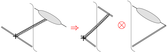
Figure 2: Factorization of the LO real soft kernel.

To obtain the leading logarithms (LL), the special vertex must appear at the outermost end of the Wilson line (nearest the final-state cut) as shown in Fig. 1(a). If the special vertex does not appear at the outermost end, the gluons emitted after the differentiated gluon must be soft too. Otherwise, their finite momenta will regularize the soft divergence associated with the differentiated gluon. In this case we will have more soft gluons, namely, a soft divergence at higher orders in the coupling constant, which corresponds to a subleading logarithm. To collect the LL in Fig. 1, the replacement $g^{\mu\nu}\to P_{J}^{\mu}l^{\nu}/(P_{J}\cdot l)$ Li (2001) is employed for the metric tensor of the differentiated gluon, where the vertex with the Lorentz index $\mu$ is located on the Wilson line, and the vertex $\nu$ on a line in the jet function. We explain this replacement by assuming that $P_{J}$ is in the plus direction for convenience. Then the component $g^{+-}$ among $g^{\mu\nu}$ leads to the leading contribution. The $+$ superscript is represented by the largest component $P_{J}^{+}$ of $P_{J}^{\mu}$ in the replacement. The components $l^{\nu}$ are arbitrary, but only $l^{-}$ is selected when $l^{\nu}$ is contracted with a vertex in the jet function, which is dominated by the momentum flow along $P_{J}$. Applying the Ward identity to the sum over all possible attachments of $l^{\nu}$ Li (2001), we factorize the differentiated gluon into the virtual soft kernel $K_{v}^{(1)}$ as displayed in Fig. 1. The factorization of the real soft kernel $K_{r}^{(1)}$ at LO is depicted in Fig. 2. The LO soft kernel $K^{(1)}$ is then written as the sum of the above two diagrams, i.e., $K^{(1)}=K_{v}^{(1)}+K_{r}^{(1)}$.

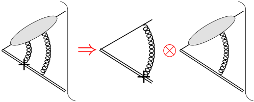
Figure 3: Diagram for the light-quark jet function with a special vertex at the innermost end of the Wilson line. The factorization gives the LO hard kernel.

To produce a LO ultraviolet divergence, the special vertex must appear at the innermost end of the Wilson line, and the differentiated gluon forms a loop correction to the quark-Wilson-line vertex as shown in Fig. 3. If this is not the case, we will have more off-shell lines, namely, a higher-order ultraviolet divergence, which leads to a subleading logarithm. The LO differentiated gluon can be factorized trivially by performing the Fierz transformation of the fermion flow,

$$I_{ij}I_{lk}=\frac{1}{4}I_{ik}I_{lj}+\frac{1}{4}(\gamma_{5})_{ik}(\gamma_{5})_{lj}+\frac{1}{4}(\gamma_{\alpha})_{ik}(\gamma^{\alpha})_{lj}+\frac{1}{4}(\gamma_{5}\gamma_{\alpha})_{ik}(\gamma^{\alpha}\gamma_{5})_{lj}+\frac{1}{8}(\sigma_{\alpha\beta})_{ik}(\sigma^{\alpha\beta})_{lj},$$ (7)

with $I$ being the identity matrix, and $\sigma_{\alpha\beta}\equiv i[\gamma_{\alpha},\gamma_{\beta}]/2$. The first and last terms contribute in the combined structure

$$I_{ij}I_{lk}\to\frac{1}{4}I_{ik}(\not\xi\not\bar{\xi})_{lj},$$ (8)

where the vector $\bar{\xi}$ lies on the light cone and satisfies $\xi\cdot\bar{\xi}=1$. The identity matrix $I_{ik}$ in Eq. (8) goes into the trace for the jet function. The matrix $(\not\xi\not\bar{\xi})_{lj}/4$ then leads to the loop integral for the hard kernel $G^{(1)}$ in Fig. 3.

The jet transverse momentum, the jet invariant mass, and the jet cone, under the factorization of the virtual differentiated gluons, remain as $P_{T}$, $M_{J}$ and $R$, respectively. The jet momentum and the jet cone are not modified by the soft real correction, but the jet invariant mass squared $M_{J}^{2}$, regarded as a small scale, is modified into $(P_{J}-l)^{2}=M_{J}^{2}-2P_{J}\cdot l$. For the light-quark jet function, we then arrive at the differential equation

$$-\frac{n^{2}}{v\cdot n}v_{\alpha}\frac{d}{dn_{\alpha}}J_{q}(M_{J}^{2},P_{T},\nu^{2},R,\mu^{2})=2(G+K)\otimes J_{q}(M_{J}^{2},P_{T},\nu^{2},R,\mu^{2}),$$ (9)

where the hard correction, the virtual soft correction, and the real soft correction to the NLO evolution kernels are written as

$$G^{(1)} = ig_{s}^{2}C_{F}\mu^{\prime\epsilon}\int\frac{d^{4-\epsilon}l}{(2\pi)^{4-\epsilon}}\frac{{\hat{n}}^{\nu}}{(n\cdot l+i\epsilon)(l^{2}+i\epsilon)}\left(\frac{1}{4}\frac{tr[\gamma_{\nu}(\not P_{J}-\not l)\not\xi\not\bar{\xi}]}{(P_{J}-l)^{2}+i\epsilon}+\frac{P_{J\nu}}{P_{J}\cdot l-i\epsilon}\right)-\delta G,$$ (10)

$$K_{v}^{(1)} = -ig_{s}^{2}C_{F}\mu^{\prime\epsilon}\int\frac{d^{4-\epsilon}l}{(2\pi)^{4-\epsilon}}\frac{{\hat{n}}\cdot P_{J}}{(n\cdot l+i\epsilon)(P_{J}\cdot l-i\epsilon)(l^{2}+i\epsilon)}-\delta K,$$ (11)

$$K_{r}^{(1)}\otimes J_{q} = g_{s}^{2}C_{F}\int\frac{d^{4}l}{(2\pi)^{4}}\frac{\hat{n}\cdot P_{J}}{(n\cdot l+i\epsilon)(P_{J}\cdot l-i\epsilon)}2\pi\delta(l^{2})J_{q}(M_{J}^{2}-2P_{J}\cdot l,P_{T},\nu^{2},R,\mu^{2}),$$ (12)

respectively. The first term in the parentheses of Eq. (10) is free of ultraviolet divergence, and the second term, representing the soft subtraction $-K_{v}^{(1)}$ to avoid double counting of the soft contribution, contains ultraviolet divergence. As adding $G^{(1)}$ and $K_{v}^{(1)}$ together, their ultraviolet divergences cancel. $K_{r}^{(1)}$ in Eq. (12) is ultraviolet finite, so the kernel $G+K=G+K_{v}+K_{r}$ is independent of renormalization scale $\mu^{\prime}$. In our regularization scheme, the additive counterterms $\delta G$ and $\delta K$ are chosen as

$$\delta G = \frac{\alpha_{s}}{2\pi}C_{F}\left[\frac{2}{\epsilon}+\ln(4\pi C_{2}^{2}\nu^{2})-\gamma_{E}\right]$$ (13)

$$= -\delta K,$$

where $\alpha_{s}=g_{s}^{2}/4\pi$, $\gamma_{E}$ is the Euler constant, and the arbitrary constant $C_{2}$ can be varied to estimate subleading logarithmic corrections to our formula.

The trace in Eq. (10) indicates that the $v^{\nu}$ term in the special vertex $\hat{n}^{\nu}$ gives a contribution suppressed by $M_{J}^{2}/P_{T}^{2}$, as compared to the contribution from the $n^{\nu}$ term. Equation (10) then reduces to

$$G^{(1)} = ig_{s}^{2}C_{F}\mu^{\prime\epsilon}\frac{n^{2}}{P_{J}\cdot n}\int\frac{d^{4-\epsilon}l}{(2\pi)^{4-\epsilon}}\left[\frac{\not n(\not P_{J}-\not l)P_{J}\cdot l}{(n\cdot l)^{2}(P_{J}-l)^{2}l^{2}}+\frac{P_{J}\cdot n}{(n\cdot l)^{2}l^{2}}\right]-\delta G,$$ (14)

$$= -\frac{\alpha_{s}}{2\pi}C_{F}\left[\ln\frac{(C_{2}\nu^{2}RP_{T})^{2}}{\mu^{\prime 2}}-1\right].$$

The virtual soft correction in Eq. (11) gives

$$K_{v}^{(1)} = -ig_{s}^{2}C_{F}\mu^{\prime\epsilon}n^{2}\int\frac{d^{4-\epsilon}l}{(2\pi)^{4-\epsilon}}\frac{2P_{J}\cdot l}{(n\cdot l)^{2}l^{2}(2P_{J}\cdot l+\lambda^{2})}-\delta K,$$ (15)

$$= \frac{\alpha_{s}}{2\pi}C_{F}\ln\frac{\lambda^{4}C_{2}^{2}}{R^{2}P_{T}^{2}\mu^{\prime 2}},$$

in which the infrared regulator $\lambda^{2}$ will be taken to be zero eventually.

It is more convenient to perform the resummation in the conjugate space via the Mellin transformation. The reason becomes evident as comparing the convolutions of the virtual and real soft corrections with the LO jet function: the former leads to $K_{v}^{(1)}\otimes J^{(0)}=K_{v}^{(1)}\delta(M_{J}^{2})$, while the latter leads to

$$K_{r}^{(1)}\otimes J_{q}^{(0)} = g_{s}^{2}C_{F}\int\frac{d^{4}l}{(2\pi)^{4}}\frac{\hat{n}\cdot P_{J}}{(n\cdot l+i\epsilon)(P_{J}\cdot l-i\epsilon)}2\pi\delta(l^{2})\delta(M_{J}^{2}-2P_{J}\cdot l),$$ (16)

$$= \frac{\alpha_{s}}{\pi}C_{F}\frac{1}{M_{J}^{2}}.$$

If transforming the above results into the Mellin space, the infrared divergences from $M_{J}\to 0$ in the virtual and real soft corrections cancel explicitly. Therefore, we introduce the Mellin transformation

$${\bar{J}}_{q}(N,P_{T},\nu^{2},R,\mu^{2})\equiv\int_{0}^{1}dx(1-x)^{N-1}J_{q}(x,P_{T},\nu^{2},R,\mu^{2}),$$ (17)

$x\equiv M_{J}^{2}/(RP_{T})^{2}$ being the dimensionless variable. The convolution in Eq. (12) is converted into a product

$$\int_{0}^{1}dx(1-x)^{N-1}K_{r}^{(1)}\otimes J_{q}={\bar{K}}_{r}^{(1)}(N){\bar{J}}_{q}(N,P_{T},\nu^{2},R,\mu^{2}),$$ (18)

with the definition

$${\bar{K}}_{r}^{(1)}(N)=g_{s}^{2}C_{F}\int_{0}^{1}dz(1-z)^{N-1}\int\frac{d^{4}l}{(2\pi)^{3}}\frac{2(P_{J}\cdot l)n^{2}}{(n\cdot l+i\epsilon)^{2}(2P_{J}\cdot l+\lambda^{2})}\delta(l^{2})\delta\left(z-2\frac{|{\bf l}|}{RP_{T}}(1-\cos\theta)\right).$$ (19)

To derive the above expression, we have made the small-mass approximation $1-\beta\cos\theta\approx 1-\cos\theta$, and inserted the identities $\int dz\delta(z-2|{\bf l}|(1-\cos\theta)/(RP_{T}))=1$ and $\int dy\delta(x-y-z)=1$. The approximation $1-x=1-y-z\approx(1-y)(1-z)$ has been also adopted, which holds in the dominant region with small $y$ and $z$.

We compute Eq. (19) by splitting it into two pieces

$${\bar{K}}_{r}^{(1)}(N) = g_{s}^{2}C_{F}\int_{0}^{1}dz[(1-z)^{N-1}-1]\int\frac{d^{4}l}{(2\pi)^{3}}\frac{n^{2}}{(n\cdot l+i\epsilon)^{2}}\delta(l^{2})\delta\left(z-2\frac{|{\bf l}|}{RP_{T}}(1-\cos\theta)\right)\Theta(R-\theta)$$ (20)

$$+g_{s}^{2}C_{F}\int_{0}^{1}dz\int\frac{d^{4}l}{(2\pi)^{3}}\frac{2(P_{J}\cdot l)n^{2}}{(n\cdot l+i\epsilon)^{2}(2P_{J}\cdot l+\lambda^{2})}\delta(l^{2})\delta\left(z-2\frac{|{\bf l}|}{RP_{T}}(1-\cos\theta)\right),$$

where the infrared regulator $\lambda^{2}$ has been neglected in the first term, because of the absence of the infrared divergence from $z\to 0$. Since the gluon momentum is finite in the first term, we require that its angle can not exceed the cone size $R$ by including the step function $\Theta(R-\theta)$, which then brings the $R$ dependence into our resummation formula. The soft effect dominates in the second term, so there is no need to constrain the range of the angle $\theta$. A straightforward calculation leads to

$${\bar{K}}_{r}^{(1)}(N) = \frac{\alpha_{s}}{\pi}C_{F}\ln\frac{R^{2}P_{T}^{2}}{\bar{N}\lambda^{2}},$$ (21)

with $\bar{N}\equiv N\exp(\gamma_{E})$. Combining Eqs. (15) and (21), we obtain

$${\bar{K}}^{(1)}(N)={\bar{K}}_{v}^{(1)}+{\bar{K}}_{r}^{(1)}(N)=\frac{\alpha_{s}}{\pi}C_{F}\left[\ln\frac{C_{1}RP_{T}}{{\bar{N}}\mu^{\prime}}+\ln\frac{C_{2}}{C_{1}}\right],$$ (22)

where ${\bar{K}}_{v}^{(1)}={K}_{v}^{(1)}$, and the dependence on the infrared regulator $\lambda^{2}$ has disappeared. Furthermore, an arbitrary constant $C_{1}$ has been introduced to estimate subleading logarithmic corrections to our formula.

Solving the renormalization-group (RG) equations,

$$\mu^{\prime}\frac{d}{d\mu^{\prime}}G=\lambda_{K}=-\mu^{\prime}\frac{d}{d\mu^{\prime}}K,$$ (23)

with the cusp anomalous dimension

$$\lambda_{K}\equiv\mu^{\prime}\frac{d}{d\mu^{\prime}}\delta K=-\mu^{\prime}\frac{d}{d\mu^{\prime}}\delta G,$$ (24)

we derive

$$K\left(\frac{C_{1}RP_{T}}{\bar{N}\mu^{\prime}},\alpha_{s}(\mu^{\prime 2})\right)+G\left(\frac{C_{2}\nu^{2}RP_{T}}{\mu^{\prime}},\alpha_{s}(\mu^{\prime 2})\right)$$

$$=K\left(1,\alpha_{s}\left(\frac{C_{1}^{2}R^{2}P_{T}^{2}}{\bar{N}^{2}}\right)\right)+G\left(1,\alpha_{s}\left(C_{2}^{2}\nu^{4}R^{2}P_{T}^{2}\right)\right)-\int_{C_{1}RP_{T}/\bar{N}}^{C_{2}\nu^{2}RP_{T}}\frac{d\mu^{\prime}}{\mu^{\prime}}\lambda_{K}(\alpha_{s}(\mu^{\prime 2})),$$

$$=\frac{C_{F}}{\pi}\alpha_{s}\left(\frac{C_{1}^{2}R^{2}P_{T}^{2}}{\bar{N}^{2}}\right)\ln\frac{C_{2}}{C_{1}}+\frac{C_{F}}{2\pi}\alpha_{s}\left(C_{2}^{2}\nu^{4}R^{2}P_{T}^{2}\right)-\int_{C_{1}/\bar{N}}^{C_{2}\nu^{2}}\frac{d\omega}{\omega}\lambda_{K}(\alpha_{s}(\omega^{2}R^{2}P_{T}^{2})).$$ (25)

With the large logarithms being removed, the LO expression for the initial condition $K(1,\alpha_{s})+G(1,\alpha_{s})$ of the RG evolution has been inserted into the last line. The cusp anomalous dimension $\lambda_{K}$ is process independent, and given, up to two loops, by

$$\lambda_{K}=\frac{\alpha_{s}}{\pi}C_{F}+\frac{1}{2}\left(\frac{\alpha_{s}}{\pi}\right)^{2}C_{F}\left[C_{A}\left(\frac{67}{18}-\frac{\pi^{2}}{6}\right)-\frac{5}{9}n_{f}\right],$$ (26)

for a light quark jet, where $n_{f}$ denotes the number of active light-quark flavors.

After organizing the large logarithms in the kernels, we solve the differential equation

$$-\frac{n^{2}}{v\cdot n}v_{\alpha}\frac{d}{dn_{\alpha}}{\bar{J}}_{q}(N,P_{T},\nu^{2},R,\mu^{2})=2\nu^{2}\frac{d}{d\nu^{2}}{\bar{J}}_{q}(N,P_{T},\nu^{2},R,\mu^{2})$$

$$=2\left[K\left(\frac{C_{1}RP_{T}}{\bar{N}\mu^{\prime}},\alpha_{s}(\mu^{\prime 2})\right)+G\left(\frac{C_{2}\nu^{2}RP_{T}}{\mu^{\prime}},\alpha_{s}(\mu^{\prime 2})\right)\right]{\bar{J}}_{q}(N,P_{T},\nu^{2},R,\mu^{2}).$$ (27)

The strategy is to evolve $\nu^{2}$ from the low value $\nu_{\rm in}^{2}=C_{1}/(C_{2}\bar{N})$ to the large value $\nu_{\rm fi}^{2}=1$, corresponding to the specific choices $n=n_{\rm in}\equiv(1,(4C_{2}\bar{N}-C_{1}R^{2})/(4C_{2}\bar{N}+C_{1}R^{2}),0,0)$ and $n=n_{\rm fi}\equiv(1,(4-R^{2})/(4+R^{2}),0,0)$, respectively. The former defines the initial condition of the jet function, which can be evaluated at a given fixed order, because of the vanishing of the logarithm $\ln(C_{2}\nu^{2}\bar{N}/C_{1})$. The latter defines the all-order jet function with the large logarithms being factorized and organized. Since the jet function collects the soft and collinear radiations, which mainly occur at a lower scale, $\mu^{2}$ should take a value of ${\mathcal{O}}(R^{2}P_{T}^{2}/{\bar{N}})$. This choice introduces an additional single logarithm, that needs to be summed to all orders by a RG evolution equation in $\mu$. To achieve it, we set $\mu^{2}\sim{\mathcal{O}}(R^{2}P_{T}^{2}/(\bar{N}\nu^{2}))$, which will be elaborated in Appendix A. The solution to Eq. (27) is derived as

$${\bar{J}}_{q}(N,P_{T},\nu_{\rm fi}^{2},R) = {\bar{J}}_{q}(N,P_{T},\nu_{\rm in}^{2},R)\exp[S_{q}(N,P_{T},R)],$$ (28)

with the Sudakov exponent

$$S_{q}(N,P_{T},R) = -\int_{C_{1}/\bar{N}}^{C_{2}}\frac{dy}{y}\left\{\int_{C_{1}/\bar{N}}^{y}\frac{d\omega}{\omega}\lambda_{K}(\alpha_{s}(\omega^{2}R^{2}P_{T}^{2}))-\frac{C_{F}}{2\pi}\alpha_{s}(y^{2}R^{2}P_{T}^{2})-\frac{C_{F}}{\pi}\alpha_{s}\left(\frac{C_{1}^{2}R^{2}P_{T}^{2}}{\bar{N}^{2}}\right)\ln\frac{C_{2}}{C_{1}}\right\}.$$ (29)

It is noted that the $R$ dependence appears in the single logarithmic term of the Sudakov exponent.

We further evolve $\alpha_{s}$ from the scale $C_{1}RP_{T}/\bar{N}$ to $yRP_{T}$ in the last term of Eq. (29),

$$-\frac{C_{F}}{\pi}\alpha_{s}\left(\frac{C_{1}^{2}R^{2}P_{T}^{2}}{\bar{N}^{2}}\right) = -\frac{C_{F}}{\pi}\left[\int_{\alpha_{s}(yRP_{T})}^{\alpha_{s}(C_{1}^{2}R^{2}P_{T}^{2}/\bar{N}^{2})}d\alpha_{s}+\alpha_{s}(y^{2}R^{2}P_{T}^{2})\right],$$ (30)

$$= C_{F}\left[\int^{yRP_{T}}_{C_{1}RP_{T}/\bar{N}}\frac{d\mu}{\mu}2\beta(\alpha_{s}(\mu^{2}))-\frac{\alpha_{s}(y^{2}R^{2}P_{T}^{2})}{\pi}\right],$$

and expand the QCD Beta function up to ${\mathcal{O}}(\alpha_{s}^{2})$, $\beta=-(\beta_{0}/4)(\alpha_{s}/\pi)^{2}$ with $\beta_{0}=11-2n_{f}/3$ Amsler et al. (2008). Inserting Eq. (30) into Eq. (29), and applying the integration by part, the exponent is rewritten as

$$S_{q}(N,P_{T},R) = -\int_{C_{1}/\bar{N}}^{C_{2}}\frac{dy}{y}\left\{A_{q}(\alpha_{s}(y^{2}R^{2}P_{T}^{2}))\ln\left(\frac{C_{2}}{y}\right)+B_{q}(\alpha_{s}(y^{2}R^{2}P_{T}^{2}))\right\},$$ (31)

with the anomalous dimensions

$$A_{q} = C_{F}\frac{\alpha_{s}}{\pi}+\frac{1}{2}C_{F}\left(\frac{\alpha_{s}}{\pi}\right)^{2}\left[C_{A}\left(\frac{67}{18}-\frac{\pi^{2}}{6}\right)-\frac{5}{9}n_{f}-\beta_{0}\ln\frac{C_{2}}{C_{1}}\right],$$

$$B_{q} = -C_{F}\frac{\alpha_{s}}{\pi}\left(\frac{1}{2}+\ln\frac{C_{2}}{C_{1}}\right).$$ (32)

The Sudakov exponent for the gluon jet function can be derived in a similar way:

$$S_{g}(N,P_{T},R) = -\int_{C_{1}/\bar{N}}^{C_{2}}\frac{dy}{y}\left\{A_{g}(\alpha_{s}(y^{2}R^{2}P_{T}^{2}))\ln\left(\frac{C_{2}}{y}\right)+B_{g}(\alpha_{s}(y^{2}R^{2}P_{T}^{2}))\right\},$$ (33)

where the anomalous dimension $A_{g}$ ($B_{g}$) is obtained by substituting $C_{A}$ for $C_{F}$ in $A_{q}$ ($B_{q}$). In this work the NLL terms have been included into the resummation by adopting $A_{f}$ at two-loop level and $B_{f}$ at one-loop level. Although the numerical evaluation of the Sudakov integral induces some next-to-next-to-leading logarithmic (NNLL) terms, the inclusion of the complete NNLL terms demands higher-order contributions to $A_{f}$ and $B_{f}$. Hence, we shall refer our resummation formalism presented here as one with the NLL accuracy. Finally, it is noted that the non-global logarithms discussed in Refs. Banfi et al. (2010); Khelifa-Kerfa (2012); Chien et al. (2013) are not included in our resummation formalism for the jet function definition in Eq. (2).

We evaluate the initial conditions of the Sudakov evolution for the light-quark and gluon jet functions up to NLO in Appendix A, and confirm that the large logarithms $\ln\bar{N}$ do not appear in these initial conditions as $\nu^{2}=\nu_{\rm in}^{2}$; namely, they have been collected into the Sudakov exponents. We note that the quark-loop contribution to the gluon jet function, which carries a different color factor, has to be handled separately as shown in the next section. The resummation formulas for the light-quark and gluon jets are summarized, in the Mellin space, as

$$\bar{J}_{q}(N,P_{T},R) = \frac{1}{R^{2}P_{T}^{2}}\left\{1+\frac{C_{F}}{\pi}\alpha_{s}\left(C_{3}^{2}R^{2}P_{T}^{2}\right)\left[\frac{1}{2}\ln\frac{C_{1}}{C_{2}}-\frac{1}{2}\ln^{2}\frac{C_{1}}{C_{2}}+\frac{1}{4}\ln\frac{C_{3}^{2}C_{1}}{C_{2}}+\frac{1}{2}\gamma_{E}-\frac{\pi^{2}}{4}-\frac{9}{8}\right]\right\}$$ (34)

$$\times S_{q}(N,P_{T},R),$$

$$\bar{J}_{g}(N,P_{T},R) = \frac{1}{R^{2}P_{T}^{2}}\left\{1+\frac{C_{A}}{\pi}\alpha_{s}\left(C_{3}^{2}R^{2}P_{T}^{2}\right)\left[\frac{1}{2}\ln\frac{C_{1}}{C_{2}}-\frac{1}{2}\ln^{2}\frac{C_{1}}{C_{2}}+\frac{5}{12}\ln\frac{C_{3}^{2}C_{1}}{C_{2}}-\frac{5}{12}\gamma_{E}-\frac{\pi^{2}}{4}+\frac{1}{2}(\ln 2-3)+\frac{1}{36}\right]\right\}$$ (35)

$$\times S_{g}(N,P_{T},R),$$

Here the third arbitrary constant $C_{3}$ has been introduced through the choice of the renormalization scale $\mu$ for the initial conditions, which denotes another source of theoretical uncertainty in our formalism.

III NUMERICAL ANALYSIS FOR JET FUNCTIONS

In this section we compare our predictions for jet mass distribution to the experimental data from the Tevatron and the LHC. As $x=M_{J}^{2}/(RP_{T})^{2}\to 0$, all moments in $N$ are equally weighted, since the suppression factor $(1-x)^{N-1}$ is not effective. The terms containing $\ln N$, being the dominant ones, have been summed to all orders in $\alpha_{s}$, so the predictions from Eqs. (34) and (35) are supposed to be reliable at small $x$. However, the running coupling constant $\alpha_{s}$, evaluated at the soft scale $RP_{T}/N$, increases with $N$, and the expansion parameter $\alpha_{s}\ln N$ may become much larger than order unity. In this region a perturbative calculation is not adequate and contributions from nonperturbative physics need to be included. Furthermore, the complex argument $\mu=yRP_{T}$ of $\alpha_{s}(\mu^{2})$ in Eqs. (31) and (33) tends to be small in magnitude at large $N$, even lower than the Landau pole scale. Therefore, in our numerical analysis we introduce a critical scale $\mu_{c}$ to avoid the Landau pole, below which the running coupling is frozen to the constant value $\alpha_{s}(\mu_{c}^{2})$. For an explicit treatment of $\alpha_{s}(\mu^{2})$, see Appendix B. As $x$ grows gradually, the large-$N$ moments are suppressed by $(1-x)^{N-1}$, and the resummation effects together with the nonperturbative inputs become less crucial. A fixed-order evaluation is then more reliable at large $x$, where Eqs. (34) and (35) are expected to coincide with the NLO jet mass distributions, cf. Appendix A.

In this work the following nonperturbative correction is implemented into the Sudakov exponent in the $N$ space

$$S_{f}^{\rm NP}(N,P_{T},R)=\frac{N^{2}Q_{0}^{2}}{R^{2}P_{T}^{2}}(C_{f}\alpha_{0}\ln N+\alpha_{1})+C_{f}\alpha_{2}\frac{NQ_{0}}{RP_{T}},$$ (36)

with $Q_{0}=1$ GeV and $C_{f}=C_{F}(C_{A})$ for the light-quark (gluon) jet function. The first two terms proportional to $N^{2}Q_{0}^{2}/P_{T}^{2}$ are similar to the singular terms in the nonperturbative contributions to the transverse-momentum resummation Collins and Soper (1981, 1982); Collins et al. (1985) and threshold resummation Li et al. (2009) formalisms. The last term, being a power correction Dasgupta et al. (1998), can be obtained from the asymptotic behavior of the Sudakov exponent. The powers in $NQ_{0}/P_{T}$ indicate that the nonperturbative effects are significant only in the extremely large $N$ region. We determine the nonperturbative parameters $\alpha_{0}$, $\alpha_{1}$ and $\alpha_{2}$ from fits to PYTHIA8.145 Sjostrand et al. (2008) predictions associated with SpartyJet Delsart et al. (2012) for the light-quark and gluon jets, separately. The resummation formulas including the nonperturbative inputs are then written as

$$\bar{J}_{q}^{\rm RES}(N,P_{T},R) = \bar{J}_{q}(N,P_{T},R)\exp[S_{q}^{\rm NP}(N,P_{T},R)],$$ (37)

$$\bar{J}_{g}^{\rm RES}(N,P_{T},R) = \bar{J}_{g}(N,P_{T},R)\exp[S_{g}^{\rm NP}(N,P_{T},R)]+\frac{n_{f}C_{F}}{3\pi R^{2}P_{T}^{2}}\alpha_{s}\left(\frac{C_{3}^{2}C_{1}R^{2}P_{T}^{2}}{C_{2}\bar{N}}\right)\left(\frac{1}{3}-\ln\frac{C_{1}C_{3}^{2}}{C_{2}}\right),$$ (38)

where the quark-loop contribution proportional to the flavor number $n_{f}$ has been added as the second term on the right-hand side of Eq. (38). Note that this contribution does not contain the large logarithm $\ln\bar{N}$ as $\mu^{2}\sim{\mathcal{O}}(R^{2}P_{T}^{2}/{\bar{N}})$, at which the final conditions of the jet functions are defined, so it is not organized into the resummation formula. The inverse Mellin transformation of the above expressions leads to

$$J_{f}^{\rm RES}(M_{J}^{2},P_{T},R)=\frac{1}{2\pi i}\int_{\rm C}dN(1-x)^{-N}\bar{J}_{f}^{\rm RES}(N,P_{T},R).$$ (39)

An appropriate contour $\rm C$ extending to infinity in the complex $N$ plane needs to be chosen for the numerical inverse transformation, which is specified in Appendix B.

As stated before, hard radiation is important at large $M_{J}$, although the probability of having a jet with large mass decreases quickly as $M_{J}$ increases. To describe the distribution at large $M_{J}$, we further perform the matching between the resummation and NLO results via

$$J_{q}^{\rm NLL/NLO}(M_{J}^{2},P_{T},R) = J_{q}^{\rm RES}(M_{J}^{2},P_{T},R)+\left[J_{q}^{(1)R}(M_{J}^{2},P_{T},R)-J_{q}^{(1)R,\rm asym}(M_{J}^{2},P_{T},R)\right],$$

$$J_{g}^{\rm NLL/NLO}(M_{J}^{2},P_{T},R) = J_{g}^{\rm RES}(M_{J}^{2},P_{T},R)+\left[J_{g}^{(1)R}(M_{J}^{2},P_{T},R)-J_{g}^{(1)R,\rm asym}(M_{J}^{2},P_{T},R)\right],$$ (40)

where $J_{f}^{(1)R}$ is the contribution from the NLO real emissions, $J_{f}^{(1)R,\rm asym}$ denotes its asymptotic expression in the $M_{J}\to 0$ limit, i.e., the so-called “singular piece” Li et al. (2011). The inclusion of the “regular piece”, i.e., the term in the square brackets on the right-hand side of Eq. (40), warrants that the expansion of $J_{f}^{\rm NLL/NLO}$ up to NLO coincides with the complete NLO QCD predictions of the jet functions. We note that the regular piece of the quark-loop contribution to the gluon jet function has been included into $J_{g}^{(1)R}-J_{g}^{(1)R,\rm asym}$, cf. Appendix A.

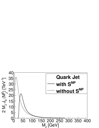
Figure 4: Quark (left) and gluon (right) jet mass distributions with $S^{\rm NP}$ (solid lines) and without $S^{\rm NP}$ (dotted lines) for $P_{T}=600$ GeV and $R=0.7$.

To be compared with the normalized jet mass distribution, we convolute Eq. (40) with the parton-level differential cross section $d\hat{\sigma}_{f}/dP_{T}$ evaluated at the renormalization scale $\mu=C_{3}RP_{T}$, the same as the initial scale in Eqs. (34) and (35), yielding the factorization formula

$$\frac{1}{\sigma}\frac{d\sigma}{dM_{J}^{2}}=\frac{1}{\sigma}\sum_{f}\int dP_{T}\frac{d\hat{\sigma}_{f}}{dP_{T}}(M_{J}^{2},P_{T})J_{f}^{\rm NLL/NLO}(M_{J}^{2},P_{T},R),$$ (41)

where $\sigma=\int(d\sigma/dM_{J}^{2})dM_{J}^{2}$ is the integrated jet cross section. We adopt the default choice $C_{1}=\exp(\gamma_{E})$, $C_{2}=\exp(-\gamma_{E})$, $C_{3}=1$, and $\mu_{c}=0.3$ GeV, and include the nonperturbative contributions in fits to PYTHIA predictions for the jet distributions with $P_{T}=600$ GeV and $R=0.7$. It is found that the nonperturbative parameter set $\alpha_{0}=-0.35$, $\alpha_{1}=0.50$ ($\alpha_{1}=-4.59$), and $\alpha_{2}=-1.66$ leads to a reasonably good fit to the light-quark (gluon) jet. It is also observed that the quark-loop contribution to the gluon jet function is negligible.

The quark and gluon jet mass distributions depicted in Fig. 4 indicate that including $S^{\rm NP}$ shifts their peak positions toward the larger jet mass region, and suppresses (enhances) the peak height of the quark (gluon) jet distribution. As stated in the Introduction, the nonperturbative contribution does not modify the behavior of the jet functions at large $M_{J}$. Given the nonperturbative parameters, we predict the jet mass distributions at any arbitrary value of collider energy $\sqrt{S}$, jet energy $P_{T}$ and jet cone size $R$. The resummation predictions for the normalized light-quark and gluon jet mass distributions as functions of $M_{J}/(RP_{T})$ for $R=0.4$, $0.5$, $0.6$ and $0.7$ with $RP_{T}=280$ GeV are presented in Fig. 5. It has been found in Ellis et al. (2008) that the NLO jet mass is remarkably well described by the simple rule-of-thumb $M_{J}\simeq 0.2RP_{T}$. However, Fig. 5 shows that not only the average jet mass but also the shapes of the light-quark and gluon jet mass distributions almost remain the same, when we vary the jet cone $R$ with $RP_{T}$ being fixed. This behavior is attributed to the fact that each component of the resummation formula, including the Sudakov factors in Eqs. (31) and (33), the initial conditions in Eqs. (34) and (35), and the nonperturbative contributions in Eq. (36), depends only on the scale $RP_{T}$. The scaling behavior is violated when the jet mass is large enough ($M_{J}/(RP_{T})>0.7$), as indicated in Fig. 5. Nevertheless, the probability to find a jet with such a large mass is low. We also note that the jet mass distribution as a function of $M_{J}/(RP_{T})$ is relatively independent of the collider energy $\sqrt{S}$, except that for substantially larger momenta the reduced phase space will lead to smaller predicted jet masses at the same momentum. Furthermore, our formalism also suggests that this conclusion holds for a similar jet (with the same $P_{T}$ and $R$) produced in any kind of hard scattering processes, such as the associated production of jets with gauge boson or Higgs boson.

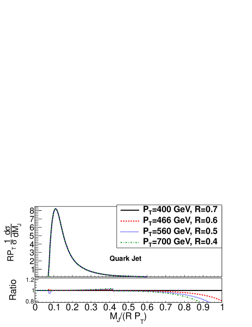
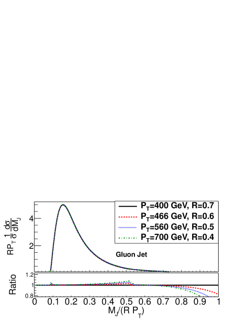
Figure 5: Resummation results for the light-quark (upper) and gluon (lower) jet mass distributions as functions of $M_{J}/(RP_{T})$ including the nonperturbative contributions for $R=0.4$, $0.5$, $0.6$ and $0.7$ with $RP_{T}=280$ GeV. The ratios relative to the predictions for $R=0.7$ are also shown.

Following Eq. (41), we convolute the light-quark and gluon jet functions with the constituent cross sections of LO partonic dijet processes at the Tevatron and the parton distribution functions (PDF) CTEQ6L Pumplin et al. (2002). Here we have neglected the soft gluon contribution Li (1997), equivalent to the soft function introduced in the Soft Collinear Effective Theory (SCET) Fleming et al. (2008), which couples the light-particle jet and the partonic processes. The resummation predictions for the jet mass distributions at $R=0.4$ and $R=0.7$ are compared to the Tevatron CDF data Aaltonen et al. (2012) in Fig. 6 with the kinematic cuts $P_{T}>400$ GeV and the rapidity interval $0.1<|Y|<0.7$ . The above data were obtained using the midpoint jet algorithm Blazey et al. (2000), and the data from the anti-$k_{t}$ algorithm Cacciari et al. (2008) do not vary much as shown in Aaltonen et al. (2012). The consistency of the resummation results with the CDF data is excellent at intermediate $M_{J}$. The resummation formula describes the shapes and the peak heights of the jet distributions in the small $M_{J}$ region, but with the peak positions being slightly lower than the CDF data. As indicated in Aaltonen et al. (2012), the PDF uncertainties could induce large variation in shapes of jet mass distributions around peak positions. The difference from the data in Fig. 6 is within the above variation. This is the first time that the pQCD factorization theorem explains the observed jet mass distributions successfully. Note that the jet mass distribution, which corresponds to the angularity distribution with $a=0$ Ellis et al. (2010), cannot be well described in the SCET formalism. In Fig. 7 we display the resummation predictions for the jet mass distributions at the Tevatron with $R=0.3$ and at the LHC with $R=0.7$, which can be tested by Tevatron data and LHC experiments.

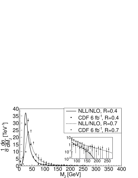
Figure 6: Comparison of resummation predictions for the jet mass distribution to Tevatron CDF data with the kinematic cuts $P_{T}>400$ GeV and $0.1<|Y|<0.7$ at $R=0.4$ and $R=0.7$. The inset shows the detailed comparison in large jet mass region.

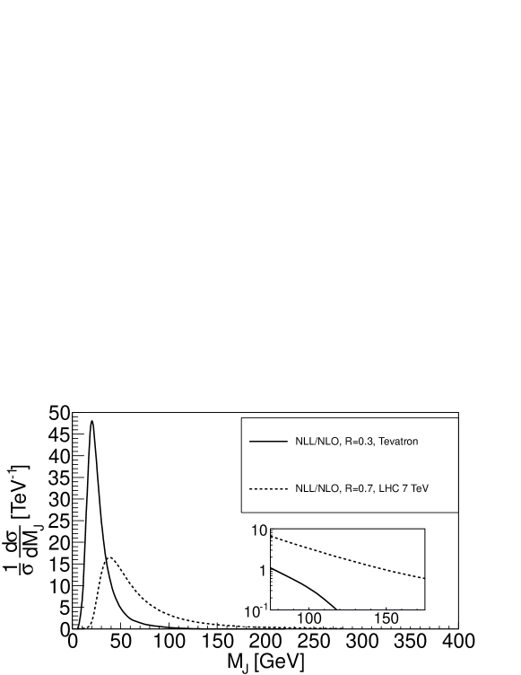
Figure 7: Resummation predictions for the jet mass distribution for Tevatron and LHC. The inset shows the detailed behaviors in large jet mass region.

IV JET ENERGY PROFILES

We define the jet energy functions $J^{E}_{f}(M_{J}^{2},P_{T},\nu^{2},R,r)$ with $f=q(g)$ denoting the light-quark (gluon), which describe the energy accumulation within the cone of size $r<R$. The definition is chosen, such that $J^{E(0)}_{f}=P_{T}\delta(M_{J}^{2})$ at LO. In this section we will study the energy profile of a light-particle jet in the framework of QCD resummation at leading power of $r$. The Feynman rules for $J^{E}_{f}$ are similar to those for the jet functions $J_{f}$ at each order of $\alpha_{s}$, except that a sum of the step functions $\sum_{i}k_{i}^{0}\Theta(r-\theta_{i})$ is inserted, where $k_{i}^{0}$ ($\theta_{i}$) is the energy (the angle with respect to the jet axis) of the final-state particle $i$. For example, the jet energy functions $J^{E}_{f}$ are expressed, at NLO, as

$$J_{q}^{E(1)}(M_{J}^{2},P_{T},\nu^{2},R,r,\mu^{2}) = \frac{(2\pi)^{3}}{2\sqrt{2}(P_{J}^{0})^{2}N_{c}}\sum_{\sigma,\lambda}\int\frac{d^{3}p}{(2\pi)^{3}2p^{0}}\frac{d^{3}k}{(2\pi)^{3}2k^{0}}[p^{0}\Theta(r-\theta_{p})+k^{0}\Theta(r-\theta_{k})]$$

$$\times{\rm Tr}\left\{\not\xi\langle 0|q(0)W_{n}^{(\bar{q})\dagger}(\infty,0)|p,\sigma;k,\lambda\rangle\langle k,\lambda;p,\sigma|W_{n}^{(\bar{q})}(\infty,0)\bar{q}(0)|0\rangle\right\}$$

$$\times\delta(M_{J}^{2}-(p+k)^{2})\delta^{(2)}(\hat{e}-\hat{e}_{\bf{p}+\bf{k}})\delta(P_{J}^{0}-p^{0}-k^{0}),$$

$$J_{g}^{E(1)}(M_{J}^{2},P_{T},\nu^{2},R,r,\mu^{2}) = \frac{(2\pi)^{3}}{2(P_{J}^{0})^{3}N_{c}}\sum_{\sigma,\lambda}\int\frac{d^{3}p}{(2\pi)^{3}2p^{0}}\frac{d^{3}k}{(2\pi)^{3}2k^{0}}[p^{0}\Theta(r-\theta_{p})+k^{0}\Theta(r-\theta_{k})]$$ (42)

$$\times\langle 0|\xi_{\sigma}F^{\sigma\nu}(0)W_{n}^{(g)\dagger}(\infty,0)|p,\sigma;k,\lambda\rangle\langle k,\lambda;p,\sigma|W_{n}^{(g)}(\infty,0)F_{\nu}^{\rho}(0)\xi_{\rho}|0\rangle$$

$$\times\delta(M_{J}^{2}-(p+k)^{2})\delta^{(2)}(\hat{e}-\hat{e}_{\bf{p}+\bf{k}})\delta(P_{J}^{0}-p^{0}-k^{0}),$$

where the expansion of the Wilson links in $\alpha_{s}$ is understood. As shown in the previous section, the quark-loop contribution to the gluon jet function is not important, cf. Eq. (38), with a proper choice of the factorization scale $\mu$ in the resummation calculation. Hence, the quark-loop contribution to the energy profile of the gluon jet can also be ignored with an appropriate choice of $\mu$.

When $r$ approaches zero, the phase space of real radiation is strongly constrained, so infrared enhancement does not cancel exactly with that in virtual contribution and results in large logarithms, e.g., $\alpha_{s}\ln^{2}r$. An evolution equation for summing these logarithms to all orders in $\alpha_{s}$ in the jet energy functions can be constructed, whose derivation is similar to that for the jet functions discussed in Sec. II: the variation of the Wilson line direction introduces the same special vertex in the differentiated jet energy functions. The virtual gluons emitted from the special vertex are factorized into the same hard kernel $G^{(1)}$ and the same virtual soft kernel $K_{v}^{(1)}$. For example, their expressions for the light-quark jet energy function $J_{q}^{E}$ are given by Eqs. (14) and (15), respectively. For the real soft gluon emitted from the special vertex, we split the sum of the step functions into

$$\sum_{i}k_{i}^{0}\Theta(r-\theta_{i})=\sum_{i^{\prime}}k_{i^{\prime}}^{0}\Theta(r-\theta_{i^{\prime}})+l^{0}\Theta(r-\theta),$$ (43)

in which $\sum_{i^{\prime}}$ means a summation over final-state particles with the real soft gluon being excluded. The first term in Eq. (43) gives

$$K_{r}^{(1)}\otimes J_{q}^{E} = g_{s}^{2}C_{F}\int\frac{d^{4}l}{(2\pi)^{4}}\frac{\hat{n}\cdot P_{J}}{(n\cdot l+i\epsilon)(P_{J}\cdot l-i\epsilon)}2\pi\delta(l^{2})\Theta\left(r-\frac{|{\bf l}|\sin\theta}{P_{T}}\right)J_{q}^{E}(M_{J}^{2}-2P_{J}\cdot l,P_{T},\nu^{2},R,r).$$ (44)

Because of the real soft gluon emission with the polar angle $\theta$, the jet axis of the rest of particles, described by $J_{q}^{E}$ on the right-hand side of the above expression, inclines by an angle $|{\bf l}|\sin\theta/P_{T}$ with respect to the jet momentum $P_{J}$. The step function in Eq. (44) imposes a phase-space constraint on the real soft gluon emission, such that the jet axis of the rest of particles cannot move outside of the jet cone $r$. Applying the Mellin transformation with respect to $x\equiv M_{J}^{2}/(RP_{T})^{2}$, we have

$$\int_{0}^{1}dx(1-x)^{N-1}K_{r}^{(1)}\otimes J_{q}^{E}={\bar{K}}_{r}^{(1)}(N){\bar{J}}_{q}^{E}(N,P_{T},\nu^{2},R,r),$$ (45)

with the definition

$${\bar{K}}_{r}^{(1)}(N) = g_{s}^{2}C_{F}\int_{0}^{1}dz(1-z)^{N-1}\int\frac{d^{4}l}{(2\pi)^{3}}\frac{2P_{J}\cdot ln^{2}}{(n\cdot l+i\epsilon)^{2}(2P_{J}\cdot l+\lambda^{2})}$$ (46)

$$\times\delta(l^{2})\delta\left(z-\frac{2|{\bf l}|}{RP_{T}}(1-\cos\theta)\right)\Theta\left(r-\frac{|{\bf l}|\sin\theta}{P_{T}}\right).$$

The second term in Eq. (43) leads to

$$K_{e}^{(1)}\otimes J_{q} = g_{s}^{2}C_{F}\int\frac{d^{4}l}{(2\pi)^{4}}\frac{\hat{n}\cdot P_{J}l^{0}\Theta(r-\theta)}{(n\cdot l+i\epsilon)(P_{J}\cdot l-i\epsilon)}2\pi\delta(l^{2})J_{q}(M_{J}^{2}-2P_{J}\cdot l,P_{T},\nu^{2},R),$$ (47)

whose Mellin transformation gives

$$\int_{0}^{1}dx(1-x)^{N-1}K_{e}^{(1)}\otimes J_{q}={\bar{K}}_{e}^{(1)}(N){\bar{J}}_{q}(N,P_{T},\nu^{2},R),$$ (48)

with the definition

$${\bar{K}}_{e}^{(1)}(N)=g_{s}^{2}C_{F}\int_{0}^{1}dz(1-z)^{N-1}\int\frac{d^{4}l}{(2\pi)^{3}}\frac{n^{2}l^{0}\Theta(r-\theta)}{(n\cdot l+i\epsilon)^{2}}\delta(l^{2})\delta\left(z-\frac{2|{\bf l}|}{RP_{T}}(1-\cos\theta)\right)\Theta\left(\frac{P_{T}}{2}-|{\bf l}|\right).$$ (49)

Strictly speaking, the energy $|{\bf l}|$ of a real gluon cannot approach infinity, so the step function at the end of the above expression has been introduced. Working out the above integration, we obtain

$${\bar{K}}_{e}^{(1)}(N) = \frac{\alpha_{s}}{2\pi}C_{F}\frac{1}{N}\int d\cos\theta\frac{n^{2}}{(n^{0}-n^{x}\cos\theta)^{2}}\frac{RP_{T}}{2(1-\cos\theta)}\left(1-\cos^{N}\theta\right)\Theta(r-\theta),$$ (50)

which is down by $1-\cos^{N}r$ and negligible in the small $r$ region. This result is attributed to the suppression of the second term in Eq. (43) by soft $l$. Hence, this piece will not be considered from now on.

The jet energy profiles are measured by summing over all jet invariant masses in experiments. Therefore, we perform a corresponding analysis with the $M_{J}^{2}$ dependence being integrated out of the jet energy profiles, namely, by considering only the $N=1$ moment. A straightforward computation leads Eq. (46) to

$${\bar{K}}_{r}^{(1)}(1) = \frac{\alpha_{s}}{2\pi}C_{F}\ln\frac{\nu^{2}R^{2}P_{T}^{4}r^{2}}{\lambda^{4}},$$ (51)

where the infrared regulator $\lambda^{2}$ will be taken to be zero eventually, and $\nu^{2}$ is defined as in Eq. (4). Using the same counterterm, Eqs. (15) and (51) are combined to form

$${\bar{K}}^{(1)}(1) = {\bar{K}}_{v}^{(1)}+{\bar{K}}_{r}^{(1)}(1)=\frac{\alpha_{s}}{2\pi}C_{F}\ln\frac{\nu^{2}P_{T}^{2}r^{2}C_{1}^{2}}{\mu^{\prime 2}}+\frac{\alpha_{s}}{2\pi}C_{F}\ln\frac{C_{2}^{2}}{C_{1}^{2}}.$$ (52)

which contains the large single logarithm $\ln r$.

Solving the RG equation for the kernels,

$$\mu^{\prime}\frac{d}{d\mu^{\prime}}G=\lambda_{K}=-\mu^{\prime}\frac{d}{d\mu^{\prime}}{\bar{K}},$$ (53)

we derive

$${\bar{K}}\left(\frac{\nu P_{T}rC_{1}}{\mu^{\prime}},\alpha_{s}(\mu^{\prime 2})\right)+G\left(\frac{\nu^{2}C_{2}RP_{T}}{\mu^{\prime}},\alpha_{s}(\mu^{\prime 2})\right)$$

$$={\bar{K}}\left(1,\alpha_{s}\left(\nu^{2}P_{T}^{2}r^{2}C_{1}^{2}\right)\right)+G\left(1,\alpha_{s}\left(\nu^{4}C_{2}^{2}R^{2}P_{T}^{2}\right)\right)-\frac{1}{2}\int_{C_{1}^{2}\nu^{2}P_{T}^{2}r^{2}}^{C_{2}^{2}\nu^{4}P_{T}^{2}R^{2}}\frac{d\mu^{\prime 2}}{\mu^{\prime 2}}\lambda_{K}(\alpha_{s}(\mu^{\prime 2})),$$

$$=\frac{C_{F}}{2\pi}\ln\frac{C_{2}^{2}}{C_{1}^{2}}\alpha_{s}\left(\nu^{2}P_{T}^{2}r^{2}C_{1}^{2}\right)+\frac{C_{F}}{2\pi}\alpha_{s}\left(\nu^{4}C_{2}^{2}R^{2}P_{T}^{2}\right)-\frac{1}{2}\int_{C_{1}^{2}\nu^{2}r^{2}}^{C_{2}^{2}\nu^{4}R^{2}}\frac{d\omega}{\omega}\lambda_{K}(\alpha_{s}(\omega P_{T}^{2})).$$ (54)

The light-quark jet energy function ${\bar{J}}_{q}^{E}$ then obeys a differential equation similar to Eq. (9):

$$-\frac{n^{2}}{v\cdot n}v_{\alpha}\frac{d}{dn_{\alpha}}{\bar{J}}_{q}^{E}(1,P_{T},\nu^{2},R,r,\mu^{2})=2\nu^{2}\frac{d}{d\nu^{2}}{\bar{J}}_{q}^{E}(1,P_{T},\nu^{2},R,r,\mu^{2})$$

$$=2\left[{\bar{K}}\left(\frac{\nu P_{T}rC_{1}}{\mu^{\prime}},\alpha_{s}(\mu^{\prime 2})\right)+G\left(\frac{\nu^{2}C_{2}RP_{T}}{\mu^{\prime}},\alpha_{s}(\mu^{\prime 2})\right)\right]{\bar{J}}_{q}^{E}(1,P_{T},\nu^{2},R,r,\mu^{2}).$$ (55)

A similar equation also holds for describing the energy profile of the gluon jet. As solving these equations, we choose the factorization scale $\mu^{2}\sim{\cal O}(r^{2}P_{T}^{2}/(R^{2}\nu^{2}))$, so that the quark-loop contribution to the gluon jet energy profile can be ignored, for the quark-loop contribution does not contain the large logarithm $\ln(R^{2}/r^{2})$ with this choice of the scale.

The strategy to solve the above equation is to evolve $\nu^{2}$ from the low value $\nu^{2}=\nu^{2}_{\rm in}\equiv C_{1}^{2}r^{2}/(C_{2}^{2}R^{2})$ to the large value $\nu^{2}=\nu^{2}_{\rm fi}\equiv 1$, which correspond to the specific choices $n=n_{\rm in}\equiv(1,(4C_{2}^{2}-r^{2}C_{1}^{2})/(4C_{2}^{2}+r^{2}C_{1}^{2}),0,0)$ and $n=n_{\rm fi}\equiv(1,(4-R^{2})/(4+R^{2}),0,0)$, respectively. The solution of the above equation is given by

$${\bar{J}}_{q}^{E}(1,P_{T},\nu_{\rm fi}^{2},R,r) = {\bar{J}}_{q}^{E}(1,P_{T},\nu_{\rm in}^{2},R,r)\exp\left[S_{q}(R,r)\right],$$ (56)

with the Sudakov exponent

$$S_{q}(R,r) = \int^{C}_{C\nu_{\rm in}^{2}}\frac{dy}{y}\left[\frac{C_{F}}{2\pi}\ln\frac{C_{2}^{2}}{C_{1}^{2}}\alpha_{s}\left(yP_{T}^{2}r^{2}C_{1}^{2}\right)+\frac{C_{F}}{2\pi}\alpha_{s}\left(y^{2}C_{2}^{2}R^{2}P_{T}^{2}\right)-\frac{1}{2}\int_{C_{1}^{2}yr^{2}}^{C_{2}^{2}y^{2}R^{2}}\frac{d\omega}{\omega}\lambda_{K}(\alpha_{s}(\omega P_{T}^{2}))\right],$$ (57)

$$= \int^{C}_{C\nu_{\rm in}^{2}}\frac{dy}{y}\left[\frac{C_{F}}{\pi}\alpha_{s}\left(y^{2}C_{2}^{2}R^{2}P_{T}^{2}\right)\left(\frac{1}{2}+\ln\frac{C_{2}}{C_{1}}\right)-\frac{1}{2}\int_{y\nu_{\rm in}^{2}}^{y^{2}}\frac{d\omega}{\omega}A_{q}(\alpha_{s}(\omega C_{2}^{2}R^{2}P_{T}^{2}))\right],$$

where the constant $C$ will be fixed below. The Sudakov exponent $S_{g}(R,r)$ for the gluon jet is obtained by substituting the color factor $C_{A}$ for $C_{F}$ in the above expression. The resummation formulas are summarized as

$${\bar{J}}_{f}^{E}(1,P_{T},\nu_{\rm fi}^{2},R,r) = {\bar{J}}_{f}^{E}(1,P_{T},\nu_{\rm in}^{2},R,r)\exp\left[S_{f}(R,r)\right],$$ (58)

with the subscript $f=q$ or $g$. The ${\cal O}(1)$ constants are chosen as $C_{1}=C_{2}=1$ and $C=\exp(5/2)$ ($C=\exp(17/6)$) in order to reproduce the single logarithm $\alpha_{s}\ln r$ in the NLO light-quark (gluon) jet energy function. The initial conditions ${\bar{J}}_{f}^{E}(1,P_{T},\nu_{\rm in}^{2},R,r)$ of the Sudakov evolution, in the absence of the large logarithms and with the factorization scale $\mu\sim{\cal O}(P_{T})$, are calculated up to NLO in Appendix D.

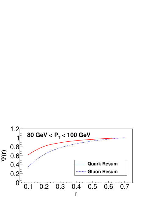
Figure 8: Resummation predictions for the energy profiles of the light-quark (solid curve) and gluon (dotted curve) jets with $\sqrt{S}=7$ TeV and 80 GeV $<P_{T}<$ 100 GeV.

Inserting the solutions in Eq. (58) into Eq. (1), the jet energy profile is written, in terms of the convolution with the parton-level differential cross section, as

$$\Psi(r)=\left[\sum_{f}\int\frac{dP_{T}}{P_{T}}\frac{d\hat{\sigma}_{f}}{dP_{T}}\bar{J}_{f}^{E}(1,P_{T},\nu_{\rm fi}^{2},R,R)\right]^{-1}\sum_{f}\int\frac{dP_{T}}{P_{T}}\frac{d\hat{\sigma}_{f}}{dP_{T}}\bar{J}_{f}^{E}(1,P_{T},\nu_{\rm fi}^{2},R,r),$$ (59)

which respects the normalization $\Psi(R)=1$, and vanishes as $r\to 0$. Note that a jet energy profile, with $N=1$, is not sensitive to the nonperturbative contribution, so our predictions are free of the nonperturbative parameter dependence, in contrast to the case of describing the jet invariant mass distribution, cf. Sec. II. We find that the light-quark jet has a narrower energy profile than the gluon jet, as exhibited in Fig. 8 for $\sqrt{S}=7$ TeV and the interval $80$ GeV $<P_{T}<$ $100$ GeV of the jet transverse momentum. The broader distribution of the gluon jet results from stronger radiations caused by the larger color factor $C_{A}=3$, compared to $C_{F}=4/3$ for a light-quark jet.

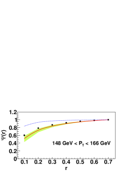
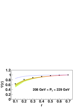
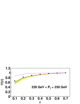
Figure 9: Comparison of resummation predictions for the jet energy profiles with $R=0.7$ to Tevatron CDF data in various $P_{T}$ intervals. The NLO predictions denoted by the dotted curves are also displayed.

We then convolute the light-quark and gluon jet energy functions with the constituent cross sections of the LO partonic subprocess and CTEQ6L PDFs Pumplin et al. (2002) at certain collider energy. The predictions are directly compared with experiment data, such as the Tevatron CDF data Acosta et al. (2005) using the midpoint jet algorithm Blazey et al. (2000), as shown in Fig. 9. The band represents the theoretical uncertainty caused by the variation of the parameters from $C_{1}=C_{2}=\exp(\gamma_{E})\approx 1.78$ to $C_{1}=C_{2}=\exp(-\gamma_{E})\approx 0.56$, which serves as an estimate of the subleading logarithmic effect that is not included in our formula. It is evident that the resummation predictions agree well with the data in all $P_{T}$ intervals. Although there is slight difference between the data and the central values of the resummation predictions, the deviation is within the theoretical uncertainty. The NLO predictions derived from $\bar{J}_{f}^{E(1)}(1,P_{T},\nu_{\rm fi}^{2},R,r)$ are also displayed for comparison, which obviously overshoot the data. The resummation predictions for the jet energy profiles are compared with the LHC CMS data at 7 TeV CMS (2010) from the anti-kt jet algorithm Cacciari et al. (2008) in Fig. 10, which are also consistent with the data in various $P_{T}$ intervals. Since we can separate the contributions from the light-quark jet and the gluon jet, the comparison with the CDF and CMS data implies that high-energy (low-energy) jets are mainly composed of the light-quark (gluon) jets. It indicates that our resummation formula has captured the dominant dynamics in a jet energy profile. Hence, a precise measurement of the jet energy profile as a function of jet transverse momentum can be used to experimentally test the production mechanism of jets in association with other particles, such as electroweak gauge bosons, top quarks and Higgs bosons.

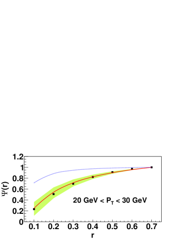
Figure 10: Resummation predictions for the jet energy profiles with $R=0.7$ compared to LHC CMS data in various $P_{T}$ intervals. The NLO predictions denoted by the dotted curves are also displayed.

A careful look at Figs. 9 and 10 reveals that the resummation predictions fall a bit below the data, as the jet transverse momentum $P_{T}$ increases. One of the reasons for this deviation may be traced back to the kinematic constraint for the real soft gluon emitted from the special vertex in Eq. (44). This constraint will include too much radiation outside the inner jet cone $r$ into the estimate of the energy profile, especially when the jet axis of the rest of particles moves toward the edge of the inner jet cone. The extra radiation can be regarded as a power correction to the energy profile in the small $r$ region, because its effect is proportional to $r$. Since more radiation will be included as $r$ increases, the energy profile at large $r$ has been overestimated in our formalism. The energy profile is normalized to unity at $r=R$, so the overestimate actually causes suppression of the distribution at small $r$, explaining the little falloff of the resummation predictions in comparison with the data. When $P_{T}$ grows, the power correction in the small $r$ region is strengthened due to the narrowness of the jet, explaining why the deviation becomes more obvious at high $P_{T}$. The above reasoning suggests a more restricted phase space for the real soft gluon in order to reduce the power correction and to improve the consistency between the predictions and the data. This subject will be investigated in a future work. Besides, we note that the effects from hadronization and underlying events on jet energy profiles have been estimated by using the PYTHIA code and removed from the published Tevatron CDF data Acosta et al. (2005). On the contrary, these effects have not been removed in the published LHC CMS data CMS (2010).

V CONCLUSION

We have developed a theoretical framework for studying jet physics based on the QCD resummation technique in this paper. The evolution equations for a light-quark jet function and for a gluon jet function have been derived and numerically solved in the Mellin ($N$) space. The inverse Mellin transformation from the $N$ space to the jet mass space was performed, which demands the inclusion of the nonperturbative contribution in the large $N$ region, in order to avoid the Landau pole, and to phenomenologically parameterize the effects from hadronization and underlying events. It has been observed that the nonperturbative contribution is crucial for describing the jet mass distribution in the low invariant mass region. The needed nonperturbative parameters were determined by fits of the resummation formula including the nonperturbative contribution to the PYTHIA predictions for the light-quark and gluon jet distributions at certain jet momentum and cone size, which were then employed to make predictions for other kinematic configurations. The above complete resummation formula, convoluted with the LO partonic hard scattering matrix elements and PDFs, have led to the jet mass distributions in good agreement with the Tevatron CDF data at different jet momenta and cone sizes. Our solutions for the light-particle jet functions are ready to be implemented into factorization formulas for jet production cross sections from various processes.

We have also derived the evolution equations for the light-quark and gluon jet energy functions. With the jet invariant mass being integrated out, the evolution equations can be straightforwardly solved in the Mellin space. The energy profiles were then predicted by convoluting the solutions with LO partonic hard scattering and PDFs. It has been checked that the resummation results for the energy profiles associated with a light-quark jet and a gluon jet agree with the PYTHIA simulations. We have demonstrated that the resummation predictions for the jet energy profiles are consistent with the Tevatron CDF data and the LHC CMS data within the theoretical uncertainty, while the NLO predictions overshoot the data. It should be emphasized that our formula for this jet substructure is insensitive to the nonperturbative contribution, and does not involve tunable parameters. Hence, the agreement with the data is a highly nontrivial success of the perturbative QCD theory. Besides, an improvement to reduce the power corrections to the predicted energy profiles can be done and will be investigated in a forthcoming paper.

Since final states observed in experiments are usually composed of quark and gluon jets, jet substructures are sensitive to the ratios between quark and gluon contributions in a given kinematic region. It is also known that the components of the quark and gluon jets are related to the initial-state PDFs. For example, the quark (gluon) jet component can be related to the initial-state gluon (quark) PDF in the $W$ boson and jet associated production. By analyzing the ratio between the quark and gluon contributions to jet substructures, we may extract additional information on the PDFs, especially on the gluon PDF in the small $x$ region. On the other hand, new physics beyond the SM introduces more hard subprocesses, which may contribute differently to quark and gluon productions in final states. Therefore, a jet substructure, e.g., the jet energy profile, can be used to search indirectly for new physics in the region, where PDFs are relatively stable, when both theoretical predictions and experiment data become precise enough.

At last, we reiterate that our framework is ready for the extension to the study of heavy-particle jets produced at the LHC, which contain energetic light decay products. For instance, a boosted top quark at the TeV scale will appear as an energetic jet, when it decays through its hadronic modes. Likewise, a boosted $W$, $Z$, or Higgs boson decaying into jet modes at the TeV scale will also appear as an energetic jet. The heavy-particle jet function and energy profile can be defined at a high energy scale in a similar way in the factorization theorem as presented in this work. The additional ingredient is the factorization of the light final states from the heavy-particle jet at the lower heavy-particle mass scale, for which the conventional heavy-quark expansion can be implemented. The solutions for the light-particle jet functions and energy profiles established in this work will serve as the inputs of this factorization formula for the heavy-particle jet. The above illustrations manifest potential and broad applications of our formalism to jet physics.

Appendix A NLO JET FUNCTIONS

In this Appendix we calculate the NLO light-quark and gluon jet functions by expanding Eq. (2) to ${\mathcal{O}}(\alpha_{s})$, and demonstrate the cancellation of infrared divergences between the virtual and real corrections in the Mellin space. After regularizing the UV divergence in the $\overline{\text{MS}}$ scheme, the NLO virtual correction to the light-quark and gluon jet functions are given by

$$J_{q}^{(1)V} = \frac{\alpha_{s}(\mu^{2})C_{F}}{\pi}\left[-\frac{1}{2}\ln^{2}\frac{4P_{T}^{2}(1-n_{x})}{\lambda^{2}(1+n_{x})}+\frac{3}{4}\ln\frac{4P_{T}^{2}(1-n_{x})}{\lambda^{2}(1+n_{x})}\right.$$ (60)

$$\left.+\frac{1}{4}\ln\frac{\mu^{2}}{R^{2}P_{T}^{2}}+\frac{1}{2}\gamma_{E}-\frac{\pi^{2}}{3}-\frac{9}{8}\right]\delta(M_{J}^{2}),$$

$$J_{g}^{(1)V} = \frac{\alpha_{s}(\mu^{2})C_{A}}{\pi}\left[-\frac{1}{2}\ln^{2}\frac{4P_{T}^{2}(1-n_{x})}{\lambda^{2}(1+n_{x})}+\frac{11}{12}\ln\frac{4P_{T}^{2}(1-n_{x})}{\lambda^{2}(1+n_{x})}\right.$$ (61)

$$\left.+\frac{5}{12}\left(\ln\frac{\mu^{2}}{R^{2}P_{T}^{2}}-\gamma_{E}\right)-\frac{\pi^{2}}{3}+\frac{1}{2}(\ln 2-3)+\frac{1}{36}\right]\delta(M_{J}^{2}),$$

respectively, where $\lambda^{2}$ is an infrared regulator, and the Wilson line direction has been chosen as $n=(1,n_{x},0,0)$ for convenience. The quark-loop contributions to the gluon jet function will be elaborated at the end of this Appendix.

The explicit expressions for the NLO real corrections to the light-quark and gluon jet functions are written as

$$J_{q}^{(1)R} = \frac{\alpha_{s}(\mu^{2})C_{F}\beta(1+\beta)}{8\pi M_{J}^{2}(\beta-n_{x})^{2}}\left\{\frac{(\beta-\cos R)(\beta-n_{x})[\beta(2n_{x}-1)+n_{x}-2]}{1-\beta\cos R}\right.$$ (62)

$$\left.+(1+\beta)^{2}(1-n_{x})^{2}\ln\frac{(1+\beta^{2})(1+n_{x}\cos R)-2\beta(n_{x}+\cos R)}{(1-\beta^{2})(1-\cos Rn_{x})}\right\},$$

$$J_{g}^{(1)R} = \frac{\alpha_{s}(\mu^{2})C_{A}\beta(1+\beta)^{2}}{96\pi M_{J}^{2}(\beta-n_{x})^{3}}\left\{\frac{(\beta-\cos R)(\beta-n_{x})}{(\beta\cos R-1)^{3}}\right.$$ (63)

$$\left.\times[\beta(\beta^{3}-3\beta+18+4(\beta^{2}-9\beta-3)\cos R+(7+18\beta-3\beta^{2})\beta\cos^{2}R)\right.$$

$$\left.+n_{x}^{2}(7\beta^{2}+18\beta-3-4\beta(3\beta^{2}+9\beta-1)\cos R+(6\beta^{4}+18\beta^{3}-3\beta^{2}+1)\cos^{2}R)\right.$$

$$\left.-2\beta n_{x}((9\beta^{3}+3\beta^{2}+9\beta+1)\cos^{2}R-2(9\beta^{2}+4\beta+9)\cos R+\beta^{2}+9\beta+3)-18n_{x}+6]\right.$$

$$\left.+3(1+\beta)^{3}(1-n_{x})^{3}\ln\frac{(1+\beta^{2})(1+\cos Rn_{x})-2\beta(\cos R+n_{x})}{(1-\beta^{2})(1-n_{x}\cos R)}\right\},$$

respectively, where the polar angle of the radiated particle momentum has been constrained to be within the cone size $R$. In the $M_{J}\to 0$ limit and without restricting the phase space of the soft radiation, i.e., with $R\to\pi$, the large logarithms in the above expressions are collected into

$$J_{q}^{(1)R,\rm asym} = \frac{\alpha_{s}(\mu^{2})C_{F}}{\pi M_{J}^{2}}\left[\ln\frac{4(1-n_{x})P_{T}^{2}}{(1+n_{x})M_{J}^{2}}-\frac{3}{4}\right],$$ (64)

$$J_{g}^{(1)R,\rm asym} = \frac{\alpha_{s}(\mu^{2})C_{A}}{\pi M_{J}^{2}}\left[\ln\frac{4(1-n_{x})P_{T}^{2}}{(1+n_{x})M_{J}^{2}}-\frac{11}{12}\right].$$ (65)

This isolation of the $R$-independent soft contributions at NLO has followed the treatment of the evolution kernel from the real soft gluon emission in Eq. (20).

Combining the NLO real and virtual corrections to the light-quark jet function in the Mellin space, we arrive at an infrared finite expression

$$\int_{0}^{1}dx(1-x)^{N-1}(J_{q}^{(1)V}+J_{q}^{(1)R,\rm asym}) = \frac{\alpha_{s}(\mu^{2})C_{F}}{\pi R^{2}P_{T}^{2}}\left[-\frac{1}{2}\ln^{2}(\nu^{2}\bar{N})+\frac{3}{4}\ln(\nu^{2}\bar{N})\right.$$ (66)

$$\left.+\frac{1}{4}\ln\frac{\mu^{2}}{R^{2}P_{T}^{2}}+\frac{1}{2}\gamma_{E}-\frac{\pi^{2}}{4}-\frac{9}{8}\right],$$

in which the infrared regulator $\lambda^{2}$ has disappeared. Those $N$-dependent terms suppressed by $1/\bar{N}$ have been dropped, whose effect is expected to be minor. Similarly, the NLO gluon jet function is given, in the Mellin space, by

$$\int_{0}^{1}dx(1-x)^{N-1}(J_{g}^{(1)V}+J_{g}^{(1)R,\rm asym}) = \frac{\alpha_{s}(\mu^{2})C_{A}}{\pi R^{2}P_{T}^{2}}\left[-\frac{1}{2}\ln^{2}(\nu^{2}\bar{N})+\frac{11}{12}\ln(\nu^{2}\bar{N})\right.$$ (67)

$$\left.+\frac{5}{12}\left(\ln\frac{\mu^{2}}{R^{2}P_{T}^{2}}-\gamma_{E}\right)-\frac{\pi^{2}}{4}+\frac{1}{2}(\ln 2-3)+\frac{1}{36}\right].$$

Applying the derivative $\nu^{2}d/d\nu^{2}$ in Eq. (27) to the above expressions, it is easy to see that the double logarithms reduce to single logarithms, which contribute to the kernel $G+K$ in Eq. (9). Since the double logarithms are $\mu^{\prime}$-independent, $G+K$ is $\mu^{\prime}$-independent, and satisfies the RG equations in Eq. (23). Choosing the renormalization scale $\mu^{2}=C_{3}^{\prime 2}R^{2}P_{T}^{2}/(\bar{N}\nu^{2})$, the above NLO jet functions become

$$\int_{0}^{1}dx(1-x)^{N-1}(J_{q}^{(1)V}+J_{q}^{(1)R,\rm asym})$$

$$=\frac{C_{F}}{\pi R^{2}P_{T}^{2}}\alpha_{s}\left(\frac{C_{3}^{\prime 2}R^{2}P_{T}^{2}}{\bar{N}\nu^{2}}\right)\left[-\frac{1}{2}\ln^{2}(\nu^{2}\bar{N})+\frac{1}{2}\ln(\nu^{2}\bar{N})+\frac{1}{4}\ln C_{3}^{\prime 2}+\frac{1}{2}\gamma_{E}-\frac{\pi^{2}}{4}-\frac{9}{8}\right],$$ (68)

$$\int_{0}^{1}dx(1-x)^{N-1}(J_{g}^{(1)V}+J_{g}^{(1)R,\rm asym})$$

$$=\frac{C_{A}}{\pi R^{2}P_{T}^{2}}\alpha_{s}\left(\frac{C_{3}^{\prime 2}R^{2}P_{T}^{2}}{\bar{N}\nu^{2}}\right)\left[-\frac{1}{2}\ln^{2}(\nu^{2}\bar{N})+\frac{1}{2}\ln(\nu^{2}\bar{N})+\frac{5}{12}\ln C_{3}^{\prime 2}-\frac{5}{12}\gamma_{E}-\frac{\pi^{2}}{4}+\frac{1}{2}(\ln 2-3)+\frac{1}{36}\right].$$ (69)

The choice of $\mu$ depends on $\nu^{2}$ in the way that we have $\mu\sim{\mathcal{O}}(RP_{T})$ as $\nu^{2}=\nu^{2}_{\rm in}\equiv C_{1}/(C_{2}\bar{N})$ for the initial conditions, which then do not contain the large logarithms $\ln\bar{N}$. The NLO initial conditions of the Sudakov evolution

$$\int_{0}^{1}dx(1-x)^{N-1}(J_{q}^{(1)V}+J_{q}^{(1)R,\rm asym})_{\rm initial}$$

$$=\frac{C_{F}}{\pi R^{2}P_{T}^{2}}\alpha_{s}\left(C_{3}^{2}R^{2}P_{T}^{2}\right)\left[\frac{1}{2}\ln\frac{C_{1}}{C_{2}}-\frac{1}{2}\ln^{2}\frac{C_{1}}{C_{2}}+\frac{1}{4}\ln\frac{C_{3}^{2}C_{1}}{C_{2}}+\frac{1}{2}\gamma_{E}-\frac{\pi^{2}}{4}-\frac{9}{8}\right],$$ (70)

$$\int_{0}^{1}dx(1-x)^{N-1}(J_{g}^{(1)V}+J_{g}^{(1)R,\rm asym})_{\rm initial}$$

$$=\frac{C_{A}}{\pi R^{2}P_{T}^{2}}\alpha_{s}\left(C_{3}^{2}R^{2}P_{T}^{2}\right)\left[\frac{1}{2}\ln\frac{C_{1}}{C_{2}}-\frac{1}{2}\ln^{2}\frac{C_{1}}{C_{2}}+\frac{5}{12}\ln\frac{C_{3}^{2}C_{1}}{C_{2}}-\frac{5}{12}\gamma_{E}-\frac{\pi^{2}}{4}+\frac{1}{2}(\ln 2-3)+\frac{1}{36}\right],$$ (71)

are derived from Eqs. (68) and (69), respectively, with $C_{3}^{2}=C_{3}^{\prime 2}C_{2}/C_{1}$. The original definitions of the jet functions in Eq. (2) involve the Wilson links on the light cone along the vector $\xi$. Setting $\nu^{2}=\nu_{\rm fi}^{2}\equiv 1$, Eqs. (68) and (69) reproduce the $\ln\bar{N}$ terms in these original definitions at NLO, leading to the final conditions

$$\int_{0}^{1}dx(1-x)^{N-1}(J_{q}^{(1)V}+J_{q}^{(1)R,\rm asym})_{\rm final}$$

$$=\frac{C_{F}}{\pi R^{2}P_{T}^{2}}\alpha_{s}\left(\frac{C_{3}^{2}C_{1}R^{2}P_{T}^{2}}{C_{2}\bar{N}}\right)\left[-\frac{1}{2}\ln^{2}\bar{N}+\frac{1}{2}\ln\bar{N}+\frac{1}{4}\ln\frac{C_{3}^{2}C_{1}}{C_{2}}+\frac{1}{2}\gamma_{E}-\frac{\pi^{2}}{4}-\frac{9}{8}\right],$$ (72)

$$\int_{0}^{1}dx(1-x)^{N-1}(J_{g}^{(1)V}+J_{g}^{(1)R,\rm asym})_{\rm final}$$

$$=\frac{C_{A}}{\pi R^{2}P_{T}^{2}}\alpha_{s}\left(\frac{C_{3}^{2}C_{1}R^{2}P_{T}^{2}}{C_{2}\bar{N}}\right)\left[-\frac{1}{2}\ln^{2}\bar{N}+\frac{1}{2}\ln\bar{N}+\frac{5}{12}\ln\frac{C_{3}^{2}C_{1}}{C_{2}}-\frac{5}{12}\gamma_{E}-\frac{\pi^{2}}{4}+\frac{1}{2}(\ln 2-3)+\frac{1}{36}\right].$$ (73)

It is seen that as the integration variable $\nu^{2}$ in Eq. (27) varies from $\nu_{\rm in}^{2}$ to $\nu_{\rm fi}^{2}$, the scale $\mu^{2}$ varies from ${\mathcal{O}}(R^{2}P_{T}^{2})$ to ${\mathcal{O}}(R^{2}P_{T}^{2}/{\bar{N}})$. The latter describes the soft and collinear radiations in the jet mass distribution appropriately, because they mainly occur at a lower scale.

The NLO terms in the expansion of the Sudakov exponent contain

$$\left.\exp[S_{f}(N)]\right|_{\alpha_{s}}=\frac{C_{f}}{\pi}\alpha_{s}\left(-\frac{1}{2}\ln^{2}\bar{N}+\frac{1}{2}\ln\bar{N}+\frac{1}{2}\ln\frac{C_{2}}{C_{1}}+\frac{1}{2}\ln^{2}\frac{C_{2}}{C_{1}}\right),$$ (74)

where $C_{f}=C_{F}$ or $C_{A}$, for $S_{q}$ or $S_{g}$, respectively. Combining the above expansion with Eqs. (70) and (71), it is straightforward to show that the resummed jet functions in Eqs. (37) and (38) indeed agree with the final conditions in Eqs. (72) and (73) at NLO, respectively. That is, our resummation formalism is matched to the NLO jet functions with $\mu^{2}\sim{\mathcal{O}}(R^{2}P_{T}^{2}/{\bar{N}})$, implying that the single logarithm introduced by our choice of $\mu^{2}$ has been also summed into the Sudakov factor. The all-order summation of this single logarithm corresponds to the RG evolution in $\mu^{2}$ from $\mu^{2}=C_{3}^{2}R^{2}P_{T}^{2}$ to $\mu^{2}=(C_{3}^{2}C_{1}R^{2}P_{T}^{2})/(C_{2}\bar{N})$.

At last, we discuss the treatment of the virtual and real quark-loop contributions to the gluon jet function

$$J_{g\to q\bar{q}}^{(1)V} = -\frac{\alpha_{s}(\mu^{2})n_{f}C_{F}}{3\pi}\left(\ln\frac{\mu^{2}}{\lambda^{2}}-\frac{1}{3}\right)\delta(M_{J}^{2}),$$ (75)

$$J_{g\to q\bar{q}}^{(1)R} = \frac{\alpha_{s}(\mu^{2})n_{f}C_{F}\beta^{3}(1+\beta)^{2}(\beta-\cos R)}{48\pi M_{J}^{2}(1-\beta\cos R)^{3}}\left[\beta^{2}(1+3\cos^{2}R)-8\beta\cos R+3+\cos^{2}R\right],$$ (76)

respectively. In the $M_{J}\to 0$ and $R\to\pi$ limits, Eq. (76) gives

$$J_{g\to q\bar{q}}^{(1)R,\rm asym} = \frac{\alpha_{s}(\mu^{2})n_{f}C_{F}}{3\pi M_{J}^{2}},$$ (77)

and the infrared finite expression

$$\int_{0}^{1}dx(1-x)^{N-1}(J_{g\to q\bar{q}}^{(1)V}+J_{g\to q\bar{q}}^{(1)R,\rm asym}) = -\frac{\alpha_{s}(\mu^{2})n_{f}C_{F}}{3\pi R^{2}P_{T}^{2}}\left(\ln\bar{N}-\frac{1}{3}+\ln\frac{\mu^{2}}{R^{2}P_{T}^{2}}\right).$$ (78)

With our choice of $\mu^{2}$, the final condition from the quark-loop contributions is written as

$$\int_{0}^{1}dx(1-x)^{N-1}(J_{g\to q\bar{q}}^{(1)V}+J_{g\to q\bar{q}}^{(1)R,\rm asym})_{\rm final}=\frac{n_{f}C_{F}}{3\pi R^{2}P_{T}^{2}}\alpha_{s}\left(\frac{C_{3}^{2}C_{1}R^{2}P_{T}^{2}}{C_{2}\bar{N}}\right)\left(\frac{1}{3}-\ln\frac{C_{1}C_{3}^{2}}{C_{2}}\right),$$ (79)

which has been added into Eq. (38). The absence of the logarithm $\ln\bar{N}$ implies that the quark-loop contribution is not important, as verified in the numerical analysis.

The initial conditions of the jet functions, namely, the prefactors of $S_{f}$ in Eqs. (34) and (35) are evaluated at the hard scale $\mu\sim{\mathcal{O}}(RP_{T})$. After applying the inverse Mellin transformation to obtain the jet functions $J_{f}^{\rm NLL/NLO}(M_{J}^{2},P_{T},R)$, which is inserted into Eq. (41) to obtain theoretical predictions, the hard scale $\mu\sim{\mathcal{O}}(RP_{T})$ remains. Since $J_{f}^{(1)V}+J_{f}^{(1)R,\rm asym}$ was organized in the resummation formalism, the regular piece $J_{f}^{(1)R}-J_{f}^{(1)R,\rm asym}$ has to be added back in order to reproduce the complete NLO corrections to the jet functions. This piece is also evaluated at the hard scale $\mu\sim{\mathcal{O}}(RP_{T})$ in Eq. (40). Similarly, the regular piece of the quark-loop contribution, $J_{g\to q\bar{q}}^{(1)R}-J_{g\to q\bar{q}}^{(1)R,\rm asym}$, should be included too, which has been combined into $J_{g}^{(1)R}-J_{g}^{(1)R,\rm asym}$ on the right-hand side of Eq. (40).

Appendix B INVERSE MELLIN TRANSFORMATION

Figure 11: Contour for the integration variable $y$ in Eqs. (31) and (33).

Because the evolution equations were solved in the Mellin space, we need to perform the inverse Mellin transformation to get the solutions in the space of the jet invariant mass. As stated in Sec. III, the argument $\mu^{2}$ of $\alpha_{s}(\mu^{2})$ in the Sudakov integrals should be treated as a complex number in the inverse Mellin transformation. Besides, the argument becomes very small (lower than the QCD scale $\Lambda_{\text{QCD}}$) in the large $N$ region, and the running coupling constant suffers the Landau pole problem Vogt (2001); Amsler et al. (2008). To avoid the Landau pole, we introduce a critical scale $\mu_{c}$, below which the running coupling constant is frozen to a constant value $\alpha_{s}(\mu_{c}^{2})$. To be precise, the following prescription is proposed

$$\alpha_{s}(\mu^{2})=\left\{\begin{array}[]{ll}\alpha_{s}(\mu_{c}^{2}\exp[2{\rm Arg}(\mu)]),&|\mu|<\mu_{c}\\ \alpha_{s}(\mu^{2}),&|\mu|>\mu_{c}\end{array}\right..$$ (82)

We have adopted the perturbative expansion of $\alpha_{s}$ in the numerical analysis

$$\alpha_{s}(Q^{2})=\frac{\alpha_{s}(\mu^{2})}{X}\left\{1-\frac{\alpha_{s}(\mu^{2})}{2\pi}\frac{\beta_{1}}{\beta_{0}}\frac{\ln X}{X}\right\},$$ (83)

with

$$X = 1+\frac{\alpha_{s}(\mu^{2})}{4\pi}\beta_{0}\ln\frac{Q^{2}}{\mu^{2}},$$

$$\beta_{0} = 11-\frac{2}{3}n_{f},\;\;\;\;\beta_{1}=51-\frac{19}{3}n_{f}.$$ (84)

The variable $N$, appearing in the lower bound of $y$ in Eqs. (31) and (33), should be also treated as a complex number in the inverse Mellin transformation. The contour in the complex $y$ plane is depicted in Fig. 11, according to which an integral over $y$ is handled in the following way,

$$\int^{C_{2}}_{C_{1}/\bar{N}}dyF(y) = \int^{C_{2}}_{C_{1}/|\bar{N}|}dy_{1}F(y_{1})+\int^{C_{1}/|\bar{N}|}_{C_{1}/\bar{N}}dy_{2}F(y_{2}),$$ (85)

$$= \int_{0}^{1}(C_{2}-C_{1}/|\bar{N}|)dt~{}F(y_{1})-\int_{0}^{1}y_{2}{\rm i}{\rm Arg}(1/\bar{N})dt~{}F(y_{2}),$$

with the variable changes $y_{1}\equiv C_{1}/|\bar{N}|+(C_{2}-C_{1}/|\bar{N}|)t$ and $y_{2}\equiv C_{1}/|\bar{N}|\exp({\rm i}{\rm Arg}(1/\bar{N})(1-t))$.

Figure 12: Conventional contour of $N$ adopted in inverse Mellin transformation.

Figure 13: Contour of $N$ adopted in our inverse Mellin transformation.

The inverse Mellin transformation for the jet function is defined as

$$J(M_{J}^{2},P_{T},\nu_{fi}^{2},R,\mu^{2})=\frac{1}{2\pi i}\int_{\rm C}dN(1-x)^{-N}\bar{J}(N,P_{T},\nu_{fi}^{2},R,\mu^{2}),$$ (86)

with $\rm C$ labelling a contour of $N$. The conventional contour of $N$ shown in Fig. 12 is not suitable for a numerical approach using a grid file, since different jet masses require different parameterizations of this contour in order to get enough information in the large $N$ region. Instead, we choose the contour depicted in Fig. 13. The inverse Mellin transformation along the upper-half part of this contour is written as

$$\frac{1}{2\pi i}\int_{C}dN(1-x)^{-N}F(N) = \frac{1}{2\pi i}\int_{0}^{\pi-\epsilon/c}N_{1}id\phi(1-x)^{-N_{1}}F(N_{1}\equiv ce^{i\phi})$$ (87)

$$+\frac{1}{2\pi i}\int_{c+i\epsilon}^{-\infty+i\epsilon}dN_{2}(1-x)^{-N_{2}}F(N_{2}),$$

$$= \frac{1}{2\pi i}\int_{0}^{1}N_{1}i(\pi-\epsilon/c)dt(1-x)^{-N_{1}}F\left[N_{1}\equiv c\exp(i(\pi-\epsilon/c)t)\right]$$

$$+\frac{1}{2\pi i}\int_{0}^{1}L\frac{-1}{(1-t)^{2}}dt(1-x)^{-N_{2}}F\left[N_{2}\equiv-c+i\epsilon+L\frac{-t}{1-t}\right].$$

The expression associated with the lower-half contour can be obtained by taking the complex conjugate of Eq. (87). The parameters involved in the integral variables $N_{1}$ and $N_{2}$ are set to $c=5$, $L=10$, and $\epsilon=10^{-6}$ in our numerical analysis.

Appendix C NLO JET ENERGY PROFILES

In this Appendix we calculate the NLO light-quark and gluon jet energy functions defined in Eq. (42). Due to their lengthy expressions, we focus only on the logarithmic terms below. The NLO virtual corrections with the factorization scale $\mu=P_{T}$ and the real corrections to the Mellin-transformed jet energy functions are given by

$$\bar{J}_{q}^{E(1),\rm V} = \frac{C_{F}\alpha_{s}}{\pi P_{T}}\left[-\frac{1}{2}\ln^{2}\frac{4P_{T}^{2}(1-n_{x})}{\lambda^{2}(1+n_{x})}+\frac{3}{4}\ln\frac{4P_{T}^{2}(1-n_{x})}{\lambda^{2}(1+n_{x})}\right],$$ (88)

$$\bar{J}_{g}^{E(1),\rm V} = \frac{C_{A}\alpha_{s}}{\pi P_{T}}\left[-\frac{1}{2}\ln^{2}\frac{4P_{T}^{2}(1-n_{x})}{\lambda^{2}(1+n_{x})}+\frac{11}{12}\ln\frac{4P_{T}^{2}(1-n_{x})}{\lambda^{2}(1+n_{x})}\right],$$ (89)

and

$$\bar{J}_{q}^{E(1),\rm R} = \frac{C_{F}\alpha_{s}}{\pi P_{T}}\left[\frac{1}{2}\ln^{2}\frac{\lambda^{2}}{P_{T}^{2}}-\left(\ln\frac{4(1-n_{x})}{(1+n_{x})r^{2}}-\frac{3}{4}\right)\ln\frac{\lambda^{2}}{P_{T}^{2}}\right.$$ (90)

$$\left.+\frac{1}{4}\ln^{2}\frac{4(1-n_{x})}{(1+n_{x})}-\frac{3}{2}\ln\frac{4(1-n_{x})}{(1+n_{x})}-\frac{1}{4}\ln^{2}r^{2}+\frac{1}{2}\ln r^{2}\ln\frac{4(1-n_{x})}{(1+n_{x})}+\frac{3}{4}\ln r^{2}\right].$$

$$\bar{J}_{g}^{E(1),\rm R} = \frac{C_{A}\alpha_{s}}{\pi P_{T}}\left[\frac{1}{2}\ln^{2}\frac{\lambda^{2}}{P_{T}^{2}}-\left(\ln\frac{4(1-n_{x})}{(1+n_{x})r^{2}}-\frac{11}{12}\right)\ln\frac{\lambda^{2}}{P_{T}^{2}}\right.$$ (91)

$$\left.+\frac{1}{4}\ln^{2}\frac{4(1-n_{x})}{(1+n_{x})}-\frac{11}{6}\ln\frac{4(1-n_{x})}{(1+n_{x})}-\frac{1}{4}\ln^{2}r^{2}+\frac{1}{2}\ln r^{2}\ln\frac{4(1-n_{x})}{(1+n_{x})}+\frac{11}{12}\ln r^{2}\right],$$

respectively. Combining the virtual and real corrections, we derive the infrared finite NLO expressions

$$\bar{J}_{q}^{E(1),\rm V}+\bar{J}_{q}^{E(1),\rm R}=\frac{\alpha_{s}C_{F}}{P_{T}\pi}\left[-\frac{1}{4}\ln^{2}\frac{4(1-n_{x})}{r^{2}(1+n_{x})}-\frac{3}{4}\ln\frac{4(1-n_{x})}{r^{2}(1+n_{x})}\right],$$ (92)

$$\bar{J}_{g}^{E(1),\rm V}+\bar{J}_{g}^{E(1),\rm R}=\frac{\alpha_{s}C_{A}}{P_{T}\pi}\left[-\frac{1}{4}\ln^{2}\frac{4(1-n_{x})}{r^{2}(1+n_{x})}-\frac{11}{12}\ln\frac{4(1-n_{x})}{r^{2}(1+n_{x})}\right],$$ (93)

in the $r\to 0$ limit, where the infrared regulator $\lambda^{2}$ has disappeared.

The singular NLO terms of the resumed jet energy functions in Eq. (56) are given by

$${\bar{J}}_{f}^{E(1)}(1,P_{T},\nu_{\rm fi}^{2},R,r)=\frac{C_{f}\alpha_{s}}{\pi P_{T}}\left[-\frac{1}{4}\ln^{2}\frac{R^{2}}{r^{2}}+\frac{1}{2}(1-\ln C)\ln\frac{R^{2}}{r^{2}}+\frac{1}{4}\ln^{2}\frac{C_{1}^{2}}{C_{2}^{2}}-\frac{1}{2}(1-\ln C)\ln\frac{C_{1}^{2}}{C_{2}^{2}}\right].$$ (94)

Substituting the vector $n_{\rm fi}\equiv(1,(4-R^{2})/(4+R^{2}),0,0)$ for $n$ in Eqs. (92) and (93) to obtain the final conditions, and choosing the ${\mathcal{O}}(1)$ constant $C=\exp(5/2)$ ($C=\exp(17/6)$) for the light-quark (gluon) jet in Eq. (94), we observe the consistency between Eqs. (92) and (93), and Eq. (94). That is, the resummation formula in Eq. (56) has collected the important logarithms in the NLO jet energy functions. The complete expressions for the NLO initial conditions corresponding to the choice $n_{\rm in}=(1,(4C_{2}^{2}-r^{2}C_{1}^{2})/(4C_{2}^{2}+r^{2}C_{1}^{2}),0,0)$, and their convolution formulas with the LO partonic subprocesses and PDFs, can be downloaded from the web site http://hep.pa.msu.edu/people/yuan/public_codes/JETENPRO/code_energy_convolute_public.zip.

References

Skiba and Tucker-Smith (2007)
W. Skiba and
D. Tucker-Smith,
Phys. Rev. D75,
115010 (2007).
Holdom (2007)
B. Holdom,
JHEP 0708, 069
(2007).
Agashe et al. (2008)
K. Agashe,
A. Belyaev,
T. Krupovnickas,
G. Perez, and
J. Virzi,
Phys. Rev. D77,
015003 (2008).
Fitzpatrick et al. (2007)
A. L. Fitzpatrick,
J. Kaplan,
L. Randall, and
L.-T. Wang,
JHEP 0709, 013
(2007).
Baur and Orr (2007)
U. Baur and
L. H. Orr,
Phys. Rev. D76,
094012 (2007).
Brooijmans et al. (2008)
G. H. Brooijmans,
A. Delgado,
B. A. Dobrescu,
C. Grojean,
M. Narain,
et al. (2008), eprint arXiv: 0802.3715
[hep-ph].
Butterworth et al. (2008)
J. M. Butterworth,
A. R. Davison,
M. Rubin, and
G. P. Salam,
Phys. Rev. Lett. 100,
242001 (2008).
Gabrielli et al. (2007)
E. Gabrielli
et al., Nucl. Phys.
B781, 64 (2007).
Almeida
et al. (2009a)
L. G. Almeida,
S. J. Lee,
G. Perez,
G. F. Sterman,
I. Sung, et al.,
Phys. Rev. D79,
074017 (2009a).
Krohn et al. (2010)
D. Krohn,
J. Thaler, and
L.-T. Wang,
JHEP 1002, 084
(2010).
Falkowski et al. (2011)
A. Falkowski,
D. Krohn,
L.-T. Wang,
J. Shelton, and
A. Thalapillil,
Phys.Rev. D84,
074022 (2011).
Krohn et al. (2011)
D. Krohn,
L. Randall, and
L.-T. Wang
(2011), eprint arXiv: 1101.0810 [hep-ph].
Fan et al. (2011)
J. Fan,
D. Krohn,
P. Mosteiro,
A. M. Thalapillil,
and L.-T. Wang,
JHEP 1103, 077
(2011).
Jankowiak and Larkoski (2011)
M. Jankowiak and
A. J. Larkoski,
JHEP 1106, 057
(2011).
Hook et al. (2012)
A. Hook,
M. Jankowiak,
and J. G.
Wacker, JHEP
1204, 007 (2012).
Krohn et al. (2009)
D. Krohn,
J. Thaler, and
L.-T. Wang,
JHEP 0906, 059
(2009).
Thaler and Wang (2008)
J. Thaler and
L.-T. Wang,
JHEP 0807, 092
(2008).
Ellis et al. (2009)
S. D. Ellis,
C. K. Vermilion,
and J. R. Walsh,
Phys. Rev. D80,
051501 (2009).
Thaler and Van Tilburg (2011)
J. Thaler and
K. Van Tilburg,
JHEP 1103, 015
(2011).
Kim (2011)
J.-H. Kim,
Phys. Rev. D83,
011502 (2011).
Stewart et al. (2010)
I. W. Stewart,
F. J. Tackmann,
and W. J.
Waalewijn, Phys. Rev. Lett.
105, 092002
(2010).
Butterworth et al. (2007)
J. Butterworth,
J. R. Ellis, and
A. Raklev,
JHEP 0705, 033
(2007).
Feige et al. (2012)
I. Feige,
M. Schwartz,
I. Stewart, and
J. Thaler,
Phys.Rev.Lett. 109,
092001 (2012).
Yang and Yan (2012)
S. Yang and
Q.-S. Yan,
JHEP 1202, 074
(2012).
Altheimer et al. (2012)
A. Altheimer,
S. Arora,
L. Asquith,
G. Brooijmans,
J. Butterworth,
et al., J.Phys.G
G39, 063001
(2012).
Acosta et al. (2005)
D. E. Acosta
et al. (CDF), Phys.
Rev. D71, 112002
(2005).
Seymour (1998)
M. Seymour,
Nucl.Phys. B513,
269 (1998).
Kidonakis et al. (1998)
N. Kidonakis,
G. Oderda, and
G. F. Sterman,
Nucl. Phys. B525,
299 (1998).
Li et al. (2011)
H.-n. Li,
Z. Li, and
C.-P. Yuan,
Phys. Rev. Lett. 107,
152001 (2011).
Collins et al. (1985)
J. C. Collins,
D. E. Soper, and
G. F. Sterman,
Nucl. Phys. B250,
199 (1985).
Ellis et al. (2010)
S. D. Ellis,
C. K. Vermilion,
J. R. Walsh,
A. Hornig, and
C. Lee,
JHEP 1011, 101
(2010).
Kelley et al. (2011)
R. Kelley,
M. D. Schwartz,
and H. X. Zhu
(2011), eprint arXiv: 1102.0561 [hep-ph].
Kelley et al. (2012)
R. Kelley,
M. D. Schwartz,
R. M. Schabinger,
and H. X. Zhu,
Phys.Rev. D86,
054017 (2012).
Almeida
et al. (2009b)
L. G. Almeida,
S. J. Lee,
G. Perez,
I. Sung, and
J. Virzi,
Phys. Rev. D79,
074012 (2009b).
Li and Yu (1996)
H.-n. Li and
H.-L. Yu,
Phys. Rev. D53,
4970 (1996).
Aaltonen et al. (2012)
T. Aaltonen et al.
(CDF Collaboration), Phys. Rev.
D85, 091101
(2012).
CMS (2010)
Report CMS–PAS–QCD–10–014
(2010).
Sjostrand et al. (2008)
T. Sjostrand,
S. Mrenna, and
P. Z. Skands,
Comput. Phys. Commun. 178,
852 (2008).
Banfi et al. (2010)
A. Banfi,
M. Dasgupta,
K. Khelifa-Kerfa,
and S. Marzani,
JHEP 1008, 064
(2010).
Khelifa-Kerfa (2012)
K. Khelifa-Kerfa,
JHEP 1202, 072
(2012).
Chien et al. (2013)
Y.-T. Chien,
R. Kelley,
M. D. Schwartz,
and H. X. Zhu,
Phys.Rev. D87,
014010 (2013).
Li (2001)
H.-n. Li,
Phys. Rev. D64,
014019 (2001).
Amsler et al. (2008)
C. Amsler et al.
(Particle Data Group), Phys.
Lett. B667, 1
(2008).
Collins and Soper (1981)
J. C. Collins and
D. E. Soper,
Nucl. Phys. B193,
381 (1981).
Collins and Soper (1982)
J. C. Collins and
D. E. Soper,
Nucl.Phys. B197,
446 (1982).
Li et al. (2009)
C. S. Li,
Z. Li, and
C.-P. Yuan,
JHEP 0906, 033
(2009).
Dasgupta et al. (1998)
M. Dasgupta,
G. E. Smye, and
B. R. Webber,
JHEP 9804, 017
(1998).
Delsart et al. (2012)
P.-A. Delsart,
K. L. Geerlings,
J. Huston,
B. T. Martin,
and C. K.
Vermilion (2012), eprint arXiv: 1201.3617
[hep-ex].
Ellis et al. (2008)
S. D. Ellis,
J. Huston,
K. Hatakeyama,
P. Loch, and
M. Tonnesmann,
Prog. Part. Nucl. Phys. 60,
484 (2008).
Pumplin et al. (2002)
J. Pumplin et al.,
JHEP 0207, 012
(2002).
Li (1997)
H.-n. Li,
Phys. Rev. D55,
105 (1997).
Fleming et al. (2008)
S. Fleming,
A. H. Hoang,
S. Mantry, and
I. W. Stewart,
Phys.Rev. D77,
074010 (2008).
Blazey et al. (2000)
G. C. Blazey,
J. R. Dittmann,
S. D. Ellis,
V. D. Elvira,
K. Frame,
et al., pp. 47–77 (2000),
eprint hep-ex/0005012.
Cacciari et al. (2008)
M. Cacciari,
G. P. Salam, and
G. Soyez,
JHEP 0804, 063
(2008).
Vogt (2001)
A. Vogt, Phys.
Lett. B497, 228
(2001).