Disk Masses at the end of the main accretion phase: CARMA Observations and Multi-Wavelength Modeling of Class I Protostars

Abstract

We present imaging observations at 1.3 mm wavelength of Class I protostars in the Taurus star forming region, obtained with the CARMA interferometer. Of an initial sample of 10 objects, we detected and imaged millimeter wavelength emission from 9. One of the 9 is resolved into two sources, and detailed analysis of this binary protostellar system is deferred to a future paper. For the remaining 8 objects, we use the CARMA data to determine the basic morphology of the millimeter emission. Combining the millimeter data with 0.9 $\mu$m images of scattered light, Spitzer IRS spectra, and broadband SEDs (all from the literature), we attempt to determine the structure of the circumstellar material. We consider models including both circumstellar disks and envelopes, and constrain the masses (and other structural parameters) of each of these components. We show that the disk masses in our sample span a range from $\lesssim 0.01$ to $\gtrsim 0.1$ M_⊙. The disk masses for our sample are significantly higher than for samples of more evolved Class II objects. Thus, Class I disk masses probably provide a more accurate estimate of the initial mass budget for star and planet formation. However, the disk masses determined here are lower than required by theories of giant planet formation. The masses also appear too low for gravitational instability, which could lead to high mass accretion rates. Even in these Class I disks, substantial particle growth may have hidden much of the disk mass in hard-to-see larger bodies.

1 Introduction

Stars form from clouds of dust and gas. As these clouds collapse and conserve angular momentum, matter that is not initially located near the polar axis falls onto a rotationally-supported disk, Most of the material that eventually makes up the star falls initially onto the disk, with some matter subsequently losing angular momentum and accreting onto the protostar. The basic picture of star formation thus involves the free-fall collapse of material from an extended envelope (or cloud) onto a disk, and then viscous accretion through the disk and onto a protostar.

At the earliest stages of collapse, one would see a roughly spherical cloud with no embedded protostar. These so-called starless cores have now been identified in a number of star forming regions (e.g., Schnee et al. 2007; Stutz et al. 2009). As collapse proceeds, a protostar and compact disk form, still surrounded by a substantial, roughly spherical envelope. Matter continues to fall onto the disk, while viscosity sources in the disk allow net outward angular momentum transport and inward mass accretion. In time the envelope completes its collapse, leaving a pre-main-sequence star surrounded by a massive disk. The disk continues to accrete onto the star, losing mass over time, eventually leaving the central pre-main sequence object surrounded by only tenuous circumstellar matter.

Each of these stages of protostellar evolution produces observational diagnostics, and an empirical picture has been developed that links evolutionary phases with properties of the emergent spectral energy distributions (Lada 1987; André et al. 1993). Class 0 objects show highly obscured SEDs that peak at sub-mm wavelengths. These are thought to be protostars still deeply embedded in massive envelopes. Class I sources show SEDs that peak in the mid-IR. Class I objects are thought to be surrounded by massive disks embedded in non-spherically-symmetric envelopes (e.g., Eisner et al. 2005). In Class II objects light from the central object is visible, although some short-wavelength emission is reprocessed and emitted at longer wavelengths. These are the T Tauri and Herbig Ae/Be stars, known to be pre-main-sequence stars surrounded by optically thick disks (e.g., Burrows et al. 1996; McCaughrean & O’Dell 1996; Corder et al. 2005). Finally, Class III sources are pre-main-sequence stars either devoid of circumstellar material or surrounded by only tenuous, optically thin circumstellar matter (e.g., Padgett et al. 2006).

The relative lengths of the Class 0, I, and II evolutionary stages can be estimated by counting the number of sources belonging to different classes in individual star-forming regions. Absolute timescales are determined by fitting the relatively unobscured Class II pre-main-sequence stellar photospheric properties to theoretical evolutionary tracks (e.g., White & Ghez 2001). The lifetime of the Class 0 phase has been estimated as $\sim 0.1$–0.2 Myr (Evans et al. 2009; Enoch et al. 2009), the Class I phase as $\sim 0.2$–0.5 Myr (Wilking et al. 1989; Greene et al. 1994; Kenyon & Hartmann 1995; Evans et al. 2009), and the Class II phase as $\sim 2$ Myr (e.g., Kenyon et al. 1990; Cieza et al. 2007).

The mass of circumstellar disks in each of the evolutionary stages outlined above has crucial implications for star and planet formation. Sufficiently massive disks may become gravitationally unstable, providing high effective viscosities and allowing rapid growth of protostellar mass. The disk mass at later stages is important to planet formation, since a certain mass is required to build giant planets (e.g., Weidenschilling 1977b).

During the Class 0 phase, disks are embedded in much more massive envelopes. High presumed infall rates ($\gtrsim 10^{-5}$ M_⊙ yr^-1; e.g., Shu 1977; Hartmann et al. 1997) from envelopes to disks likely mean that these disks are gravitationally unstable. At the Class I stage, envelopes are less massive and the disks may dominate the total system mass (e.g., Jørgensen et al. 2009). Disks in Class II objects generally appear gravitationally stable, accreting material slowly onto their central objects ($\dot{M}\lesssim 10^{-7}$ M_⊙ yr^-1; e.g., Basri & Bertout 1989; Hartigan et al. 1995). Class I sources thus offer the prospect of observing disks at an intermediate state when they may transitioning from roiling, gravitationally unstable disks, to more stable disks that could provide a hospitable environment for the early stages of planet formation.

The masses of disks surrounding Class I sources have been constrained previously using millimeter wavelength observations (e.g., Hogerheijde 2001; Osorio et al. 2003; Wolf et al. 2003; Eisner et al. 2005; Jørgensen et al. 2007, 2009). Because much of the circumstellar dust around Class I objects is expected to be optically thin, the observed millimeter flux is correlated with mass. However knowledge of the dust opacity and temperature (as a function of radius) is needed in order to convert flux to mass. Moreover, dense regions (e.g., close to the central protostars) may be optically thick. Radiative transfer modeling of multi-wavelength data is required to disentangle these effects and provide unambiguous circumstellar mass estimates.

Historically, constraints on the circumstellar matter in Class I sources came from modeling of SEDs (e.g., Adams et al. 1987; Kenyon et al. 1993a; Robitaille et al. 2007). These models include flattened, disk-like distributions of matter that are a consequence of angular momentum conservation (e.g., Ulrich 1976; Terebey et al. 1984). However, the SED data can often be explained with different models as well, including edge-on flared disk models (e.g., Chiang & Goldreich 1999). Imaging data, including scattered light images (e.g., Whitney et al. 2003) or millimeter images of continuum and line emission (e.g., Jørgensen et al. 2007, 2009), have also been used to constrain the circumstellar structure of Class I sources.

Modeling a single dataset—e.g., an SED or scattered light image—is subject to ambiguities. Modeling multi-wavelength images and fluxes simultaneously provides tighter constraints on geometry, since emission at different wavelengths arises in different layers of circumstellar material. Scattered light at short wavelength traces low-density surface layers, while longer-wavelength (e.g., millimeter) emission arises in deeper, denser regions. Such modeling has been applied to a number of Class I sources, yielding constraints on circumstellar morphology better than afforded by modeling any single dataset (Osorio et al. 2003; Wolf et al. 2003; Eisner et al. 2005).

Previous estimates of disk masses in Class I objects cover a broad range. Modeling millimeter images together with SEDs and scattered light images, disk masses of 0.01–1 M_⊙ (with most masses $\gtrsim 0.1$ M_⊙) were determined for a handful of Class I objects (Osorio et al. 2003; Wolf et al. 2003; Eisner et al. 2005). Somewhat lower masses, spanning $\lesssim 0.01$ up to $\sim 0.05$ M_⊙, were inferred from radiative transfer modeling of sub-millimeter continuum images of 10 Class I sources (Jørgensen et al. 2009) . Some disk mass estimates are consistent with simulations of protostellar evolution, which find disk masses of $\sim 0.2$ M_⊙ for Class I objects (Vorobyov 2011). For many objects, however, estimated disk masses are substantially lower.

For some objects, mass estimates place Class I disks near the limit of gravitational stability. This finding would fit naturally into the scenario of burst-mode accretion onto Class I protostars (Vorobyov & Basu 2005), and explain the discrepant infall rates from the envelope to the disk and from the disk onto the star (e.g., Kenyon & Hartmann 1987; White & Hillenbrand 2004). In a broader sense, the implied gravitational instability provides an easily-explained viscosity source to enable angular momentum transport in protostellar disks.

Estimated disk masses in Class Is appear higher than the disk masses determined for Class II objects. The median mass of disks in nearby star-forming regions is estimated as $\sim 0.005$ M_⊙ (e.g., Andrews & Williams 2005, 2007; Eisner et al. 2008). These disks are about an order of magnitude less massive than the minimum mass solar nebula (MMSN; Weidenschilling 1977b), suggesting that many stars in the Galaxy lack the circumstellar mass needed to form solar systems like ours. Higher inferred masses in Class I disks suggest that substantial particle growth (which depletes the observable population of small dust grains) has occurred between the Class I and II stages. Planet formation may already have advanced significantly during the first million years of disk evolution. Given the short lifetimes of particles with sizes of a few centimeters to a few meters (Weidenschilling 1977a), this would imply growth of large planetesimals in less than $\sim 1$ Myr.

Substantial uncertainties remain in the estimated Class I disk masses, placing the conjectures above on somewhat shaky footing. Our aim in this paper is to better constrain the disk masses around a relatively large sample of Class I sources. We will improve upon previous constraints using high angular resolution millimeter imaging from CARMA. We model these data together with existing data at other wavelengths, including broadband SEDs, Spitzer IRS spectra, and I-band images of scattered light.

2 Observations

2.1 Sample Selection

Our sample consists of Class I sources in Taurus (Table 1). We selected objects with existing 0.9 $\micron$ scattered light imaging (Eisner et al. 2005), Spitzer IRS spectra (Furlan et al. 2008, 2011), and well-sampled SEDs (e.g., Robitaille et al. 2007, and references therein). We choose among these the targets whose previously measured fluxes at millimeter wavelengths are $>50$ mJy (Motte & André 2001). We apply this flux cut to facilitate detection and mapping of millimeter emission at high angular resolution (§2.2). However the high fluxes in previous low resolution observations do not guarantee high fluxes in a smaller beam, as extended emission would be resolved out.

While the flux cut applied to the sample may lead to a bias toward higher circumstellar masses, this bias appears to be small. The mean 1.3 mm flux density for our sample, as measured by Motte & André (2001), is $\sim 270$ mJy. If we exclude the very luminous IRAS 04287+1801 (also known as L1551 IRS 5), then the mean 1.3 mm flux density is $\sim 130$ mJy. For all of the Taurus Class I sources in Motte & André (2001), the mean flux density is $\sim 190$ mJy, or $\sim 140$ mJy excluding IRAS 04287+1801. The flux distribution of our sources is thus not significantly different than the underlying population of Taurus protostars.

IRAS 04263+2426 (also known as GV Tau or Haro 6-10) is a $1\hbox to0.0pt{.\hss}^{\prime\prime}2$ separation binary (Leinert & Haas 1989; Koresko 2002; Doppmann et al. 2008), clearly resolved into two sources in our millimeter-wavelength observations. While we provide basic properties of the binary, we do not include this object in our detailed analysis and modeling. The binarity complicates the analysis, but also provides an opportunity to study two (presumably) coeval sources. We plan to devote a separate publication to this interesting object.

2.2 CARMA Imaging

We obtained images at 1.3 mm wavelengths for our sample using the Combined Array for Research in Millimeter-wave Astronomy (CARMA). CARMA consists of six 10.4 m and nine 6.1 m antennas. During our observations the antennas were in the “C”-configuration, which provides baseline separations between 30 and 350 m. The C array observations thus provide an angular resolution of $\sim 0\hbox to0.0pt{.\hss}^{\prime\prime}8$, with sensitivity to emission on angular scales smaller than $\sim 10^{\prime\prime}$.

Some of our continuum observations were obtained before the full correlator implementation, and used 2 GHz of continuum bandwidth. Later observations were taken with the full 8 GHz of continuum bandwidth. A log of observations is given in Table 1.

We used MIRIAD (Sault et al. 1995) to calibrate the CARMA data. Bandpass calibration utilized observations of bright, (nearly) spectrally flat sources (see Table 1). To calibrate time-dependent instrumental and atmospheric effects, we observed the blazar 3C 111 every 20 minutes. In between 3C 111 observations, we obtained data on two or three targets. Because our targets are bright enough to be detected in less than a full “track” (i.e., the length of time the source is above a reasonable elevation angle), we observed multiple targets in each track. Targets in a single track shared calibrators, and comparison of calibrated data for these targets provides a consistency check on the calibration procedure. In a few of the tracks, Uranus was observed and used to set the instrumental flux scale. For the other tracks we took the flux of the gain calibrator, 3C 111, directly from the SMA submillimeter calibrators page, extrapolating to our observing date when necessary.

Baselines with abnormally noisy phases or high system temperatures were deleted. In many cases, the deleted baselines included the longest ones, and hence the angular resolution of our observations is somewhat less than the highest resolution possible with CARMA’s C-array. The longest useable baselines in our data are typically $<250$ m.

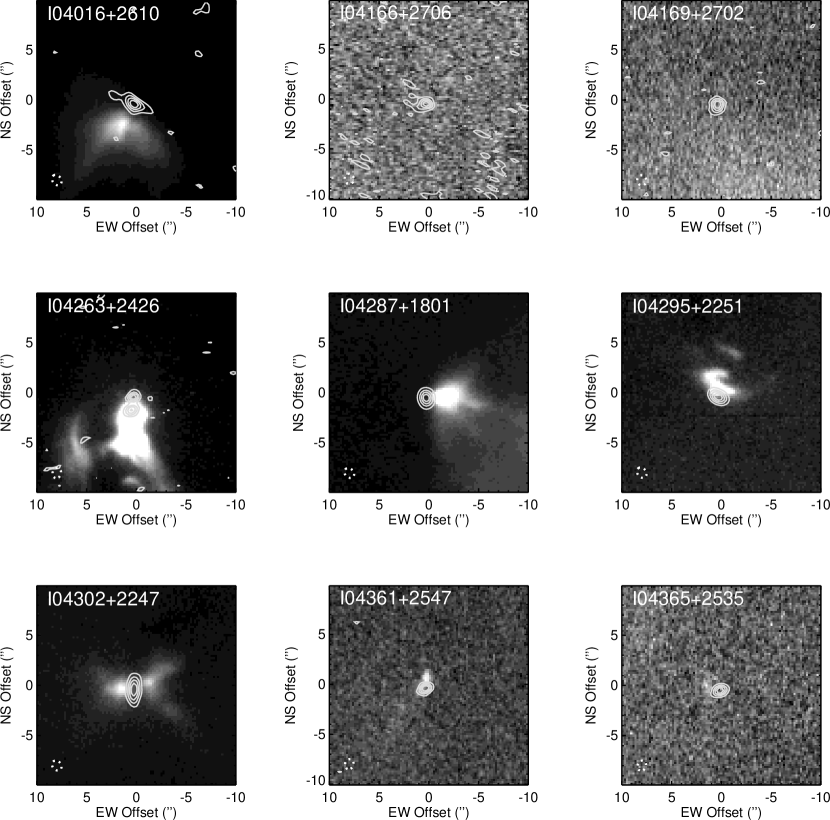
Figure 1: I-band scattered-light images in grayscale with millimeter images overplotted as contours. Contours are plotted in intervals of 20% of the peak flux. The dashed ellipse at the bottom left is the FWHM of the synthesized beams of the CARMA observations.

After passband, flux, and gain calibration, we INVERTed the Fourier data and created images. We also CLEANed the images, determined the correct PSF for the hybrid (6-meter and 10-meter dishes) CARMA array, and restored the final images using this PSF. For one of our targets, IRAS 04181+2654, no emission was detected in the map. For all other targets, the mapped emission is shown in contour plots in Figure 1. Properties of the millimeter images, including peak fluxes, 1$\sigma$ noise levels, absolute coordinates, and PSF FWHM dimensions, are listed in Table 2.

While the images are useful for visualization, the visibility data themselves are used in our analysis. Because they are the actual data, their uncertainties are better characterized than those of Fourier transformed, CLEANed images. We average the visibility data on a two-dimensional grid of $u$ and $v$ for subsequent comparison with synthetic visibility data from models. We compute weighted averages in each bin, using the weights output by MIRIAD.

The error in each bin is given by the weighted standard deviation in the mean, scaled by a factor that produces reasonable overall error bars. We select scale factors so that the error bars are similar in magnitude to the standard deviations in the means of unweighted data. For our data, we use a scale factor of five for all objects except IRAS 04287+1801, where we use a scale factor of two.

Averaged visibilities for our targets are shown in Figure 2. The visibilities computed by averaging over a two-dimensional grid of $u$ and $v$ are generally quite noisy. Azimuthally averaging these visibilities lowers the noise substantially and allows radial structure to be more easily discerned. We therefore plot the azimuthally averaged visibility amplitudes as well.

We fit inclined uniform disk models (e.g., Eisner et al. 2004) to the two-dimensional CARMA visibilities, to provide rough constraints on the geometry of the millimeter emission. We did not fit a uniform disk model to IRAS 04263+2426 because it is a binary. The fitted fluxes, sizes, inclinations, and position angles of these disk models are listed in Table 3. These fits show that the emission from most of our sample is resolved well in our observations. However, IRAS 04166+2706 appears to be unresolved, and the data for IRAS 04169+2702 and IRAS 04361+2547 lack the signal-to-noise and $uv$ coverage needed to constrain the geometry well.

2.3 Scattered Light Images

In our modeling we use Keck $I$-band imaging of our sample, published previously in Eisner et al. (2005). We calibrate the astrometry of these images by registering to the 2MASS coordinate system. In each of our $I$-band images we searched for stars also seen in 2MASS images. We then computed a plate solution for our $I$-band images. The residuals in these fits are typically smaller than $0\hbox to0.0pt{.\hss}^{\prime\prime}3$, which is comparable to the error in the 2MASS astrometry. For the angular resolution and signal-to-noise of our millimeter observations, we expect positional uncertainties of $\lesssim 0\hbox to0.0pt{.\hss}^{\prime\prime}1$ for the millimeter images. The registration of $I$-band and millimeter images is thus uncertain by $\lesssim 0\hbox to0.0pt{.\hss}^{\prime\prime}5$.

For IRAS 04263+2426 we were unable to find enough reference stars to compute a plate solution. This dearth of reference stars is caused, in part, by the shorter integration time on this bright $I$-band object (60 seconds, compared to 120–300 seconds for the other objects in our sample). For this source we attempted to line up the scattered light structure seen in $J$-band 2MASS imaging with the structure seen in the $I$-band data. We estimate uncertainties of $\sim 1^{\prime\prime}$ in this procedure.

The $I$-band images, registered to the 2MASS coordinate system, are plotted in Figure 1. The scattered light morphologies for our sample vary widely, from bright, extended emission for IRAS 04016+2610, IRAS 04263+2426, IRAS 04287+1801, IRAS 04295+2251, and IRAS 04302+2247; to weak, more compact emission for IRAS 04361+2547 and IRAS 04365+2535; to a lack of any detectable scattered light towards IRAS 04166+2706 and IRAS 04169+2702.

2.4 Spectral Energy Distributions

We compiled broadband spectral energy distributions, including Spitzer IRS spectra (Furlan et al. 2008, 2011), from the literature (Myers et al. 1987; Weaver & Jones 1992; Barsony & Kenyon 1992; Kenyon & Hartmann 1995; Padgett et al. 1999; Chandler & Richer 2000; Young et al. 2003; Moriarty-Schieven et al. 1994; Hogerheijde & Sandell 2000; Motte & André 2001; Andrews & Williams 2005; Kessler-Silacci et al. 2005; Eisner et al. 2005; Hartmann et al. 2005; Robitaille et al. 2007; Rebull et al. 2010). We ignore the error bars quoted for these photometric measurements (when available), and instead adopt a uniform uncertainty level. We adopt 10% errors for all photometric data. However, this value is somewhat arbitrary. As described in §3.3, we specify weights for various datasets in our modeling, and these weights effectively overrule the normalization of the internal uncertainties in a given dataset.

3 Modeling

Following previous work (e.g., Eisner et al. 2005), we consider a model that includes a rotating, collapsing envelope with an embedded, hydrostatic, Keplerian disk. We describe the density distribution of this model in §3.1. We use the two-dimensional Monte Carlo radiative transfer code RADMC (Dullemond & Dominik 2004) to compute the temperature distribution of our models. With the density and temperature distributions computed, we use RADMC to produce 0.9 $\mu$m images, 1.3 mm images, and SEDs spanning wavelengths from 0.1 $\mu$m to 1 cm. We convert the 1.3 mm images to two-dimensional visibilities over the same grid used to average the CARMA visibility data (§2.2). For ease of plotting, we also azimuthally average these 2D visibilities.

In all of our models we fix the dust opacities. We use dust opacities that were computed to fit extinction measurements in dense cores observed as part of the C2D project (Pontoppidan, private communication; see also Shirley et al. 2011). These opacities are computed for spherical dust grains with a size distribution described by Weingartner & Draine (2001). The dust is a mixture of approximately 30% amorphous Carbon, with grains between $6\times 10^{-4}$ and 7 $\mu$m, and 70% Silicate, with grains between $6\times 10^{-4}$ and 0.6 $\mu$m. The grains are covered with ice mantles (70% H₂O, 30% CO₂), with an assumed ice abundance of $3\times 10^{-4}$ per H₂ molecule. Changing dust opacities would affect the modeling, but we lack the computational power to vary these in concert with other parameters describing the stellar and circumstellar properties.

We consider three values of source luminosity in our analysis: 1, 3, and 10 L_⊙. Note that these are rough approximations of the true luminosities of our targets, which may lie between sampled values, but computational resources limit us to a few values. We take the stellar mass and temperature to be fixed in our modeling: $M_{\ast}$=0.5 M_☉ and $T_{\ast}$=4000 K. These values are compatible with dynamical mass estimates and effective temperature measurements (e.g., Hogerheijde 2001; White & Hillenbrand 2004). Thus, we are assuming in our modeling that the only stellar parameter that varies is the radius.

A range of viewing geometries are considered. We allow models to be inclined between 0 and 90^∘ with respect to the plane of the sky, and to have position angles spanning the full range from 0 to 360^∘. The position angle is defined east-of-north.

In §3.2, we present a parameter study that shows how synthetic data are affected by changes in various parameters. Varied parameters include properties of the circumstellar mass distribution (§3.1), protostellar luminosity, and viewing geometry. In §3.3, we describe the grid of models we computed, and discuss the procedure by which the best-fit model is found.

3.1 Input Density Distribution and Stellar Parameters

Our model includes both a collapsing envelope and an embedded disk. The density distributions of the two components are computed separately and then added together to produce the final model. We describe each of these components in turn, and demonstrate the effects of changing input parameters on synthetic data.

3.1.1 Collapsing Envelope

When a rotating, initially spherical cloud of material collapses, angular momentum conservation leads to a non-spherically symmetric distribution. Following Ulrich (1976), the density distribution of a rotating, infalling envelope is

$$\rho_{\rm env}(r,\theta)=\frac{\dot{M}}{4\pi}(GM_{\star}r^{3})^{-1/2}\bigg{(}1+\frac{\mu}{\mu_{0}}\bigg{)}^{-1/2}\bigg{(}\frac{\mu}{\mu_{0}}+2\mu_{0}^{2}\frac{R_{\rm c}}{r}\bigg{)}^{-1}.$$ (1)

Here $r$ is the stellocentric radius, $\dot{M}$ is the mass infall rate, $M_{\star}$ is the stellar mass, $\mu=cos(\theta)$, $\theta$ is the angle from the polar axis, $\mu_{0}=cos(\theta_{0})$, and $\theta_{0}$ is the initial angle of infalling material. The centrifugal radius, $R_{\rm c}$, is the location where material becomes rotationally supported against gravity and the density structure becomes less spherically distributed and more flattened:

$$R_{c}=\frac{R_{0}\Omega^{2}}{GM_{\rm env}}.$$ (2)

Here $R_{0}$ is the initial radius of the infalling matter, $\Omega$ is the angular velocity, and $M_{\rm env}$ is the envelope mass. In our modeling, we will leave the centrifugal radius as a free parameter.

For each point in the envelope, matter can only have arrived from a specific initial location. We can therefore solve for $\mu_{0}$. The particle trajectories obey the relation (see, e.g., Ulrich 1976)

$$\frac{r}{R_{c}}=\frac{\cos\theta_{0}\sin\theta_{0}^{2}}{\cos\theta_{0}-\cos\theta}=\frac{1-\mu_{0}^{2}}{1-\mu/\mu_{0}}.$$ (3)

There are three solutions to this equation. We require that the solution be real and that $\sin\theta_{0}$ and $\sin\theta$ have the same sign. This means that a particle that starts out in one quadrant of the model is required to remain in that quadrant. The analytic solution is:

$$\mu_{0}=\xi-\frac{(r-R_{c})}{3R_{c}\xi},$$ (4)

where $\xi$ is given by

$$\xi=\frac{\bigg{[}27\mu rR_{c}^{2}+\sqrt{729\mu^{2}r^{2}R_{c}^{4}+108R_{c}^{3}(r-R_{c})^{3}}\bigg{]}^{1/3}}{2^{1/3}3R_{c}}.$$ (5)

We modify this envelope model to include an outflow cavity along the rotation axis. We specify this cavity as

$$\rho_{\rm cav}(r,z>z_{0}+r^{\zeta})=\rho_{\rm env}\times f_{\rm cav}.$$ (6)

Here $z$ is the height above the midplane, $r$ is the stellocentric radius in the midplane, $z_{0}$ is the height above the midplane where the cavity begins, and $\zeta$ describes the shape and opening angle of the cavity. For simplicity we fix $z_{0}=1$ AU in our models, but we explore the effects of $\zeta$ and $f_{\rm cav}$ on synthetic data below.

The total envelope mass, $M_{\rm env}$, is obtained from the integral of $\rho_{\rm env}$. Since $M_{\rm env}\propto\rho_{\rm env}\propto\dot{M}$ (Equation 1), we may use the total envelope mass as a free parameter instead of $\dot{M}$. The envelope mass is more relevant for our purposes, since it allows a more direct comparison with the disk mass, $M_{\rm disk}$.

3.1.2 Flared Disk

The flared disk model was first described by Shakura & Sunyaev (1973), where the density distribution is given by

$$\rho_{disk}(r,z)=\rho_{0}\bigg{(}\frac{r}{r_{0}}\bigg{)}^{-\alpha}\textrm{exp}\bigg{(}-\frac{1}{2}\bigg{[}\frac{z}{h(r)}\bigg{]}^{2}\bigg{)}.$$ (7)

Here $r$ is the radial distance from the star, $z$ is the vertical distance above the midplane, and $r_{0}$ is assumed to be 1 AU. The scale height above the disk is given by

$$h(r)=h_{\rm 1AU}\bigg{(}\frac{r}{1\>{\rm AU}}\bigg{)}^{\beta}.$$ (8)

We adopt $\beta$=58/45, which is expected for a flared disk in hydrostatic equilibrium (e.g., Chiang & Goldreich 1997). This allows us to also fix the exponent of the radial volume density profile to $\alpha=3(\beta-\frac{1}{2})=$2.37 based on viscous accretion theory (Shakura & Sunyaev 1973). Note that this implies that the surface density, $\Sigma(r)\propto r^{-1.37}$. The value of $\alpha$ is similar to assumed values in previous modeling of circumstellar disks (e.g. D’Alessio et al. 1999; Chiang & Goldreich 1997), and to the inferred value for the protosolar nebula (Weidenschilling 1977b). The free parameters for the flared disk are $M_{\rm disk}$, $R_{\rm disk}$, and $h_{\rm 1AU}$. We assume that $R_{\rm disk}=R_{\rm c}$.

3.1.3 Disk+Envelope

To produce a disk+envelope model, we take the envelope model from §3.1.1 and the disk model from §3.1.2 and add their density distributions. In our modeling we vary the disk and envelope masses so that our models encompass both disk-dominated and envelope-dominated morphologies.

3.2 Parameter Study

Here we vary the input parameters of the disk+envelope model described above, and illustrate the effect these parameters have on synthetic SEDs, 0.9 $\mu$m scattered light images, and millimeter wavelength visibilities. We vary parameters about a baseline model, which has the following parameters: $M_{\rm disk}=0.1$ M_⊙, $h_{\rm 1AU}=0.05$ AU, $R_{\rm disk}=R_{\rm c}=30$ AU, $M_{\rm env}$ = 0.05 M_⊙, $R_{\rm out}=1000$ AU, $f_{\rm cav}=0.2$, $\zeta=1.0$, $L=3$ L_⊙, $i$=45^∘, and PA=$90^{\circ}$.

3.2.1 Disk Parameters

In our disk+envelope model we have assumed a power-law radial surface density profile declining with radius with an exponent of -1.37. Since the disk surface area grows as the square of radius, the radial mass distribution increases with radius: $M(r)\propto r^{0.63}$. However since the disk outer radius is equal to the envelope centrifugal radius, material in the disk is still compact compared to the envelope mass distribution. Note, too, that the temperature is higher at smaller radii, and the flux from optically thin material can still be centrally concentrated even if the mass distribution is weighted to larger radii.

A higher mass corresponds to an increased mm-wavelength flux. As seen in Figure 3, the long-wavelength SED as well as the normalization of the mm-wavelength visibility is increased as the disk mass is increased. The disk emission is unresolved for our baseline disk model radius ($R_{\rm disk}=30$ AU). However for $R_{\rm disk}\gtrsim 100$ AU, some disk emission may be resolved on the longest baselines.

The effect of disk mass on the scattered light image is small since most of the scattered light is generated on larger scales where the envelope component dominates. Figure 3 shows a slightly less extended scattered light morphology for the highest disk mass considered. However this may reflect the fact that fewer photons escaped the high optical depth during the radiative transfer calculation.

Larger disk scale heights mean that the disk is better at intercepting short-wavelength light and reprocessing it to longer wavelengths. Thus models with higher values of $h_{\rm 1AU}$ show depressed optical/near-IR fluxes and increased millimeter fluxes (Figure 4). Scattered light images become more compact for larger values of $h_{\rm 1AU}$, because photons can be scattered from vertically-extended disk regions at smaller radii.

A larger disk outer radius means more resolved millimeter visibilities (Figure 5). Larger disks also re-distribute mass to larger radii, thus decreasing the optical depth at small radii and allowing more infrared emission to escape. Because the disk outer radius is also the envelope centrifugal radius in our model, its effects on the synthetic data are somewhat more complicated. We discuss how centrifugal radius impacts the synthetic data below.

The disk surface density profile may also influence the observed radial profile of 1 mm emission, since the mostly-optically-thin dust emission correlates with mass. Shallower radial surface density profiles produce more millimeter emission at larger stellocentric radii, and hence more resolved visibilities. However, in the interest of minimizing the number of free parameters, we consider the surface density to be fixed in our modeling.

3.2.2 Envelope Parameters

Increasing the envelope mass increases the extinction toward the central object, thus decreasing the optical and infrared fluxes, and increases the mass of cooler material, thus increasing the millimeter fluxes (Figure 6). Unlike the disk mass, envelope mass is distributed over larger spatial scales, and much of the additional millimeter emission is resolved by the long-baseline CARMA observations. Increasing the envelope mass thus tends to increase the visibility amplitudes more at shorter baselines than at longer baselines.

We see in Figure 6 that the effect on the synthetic scattered light images of changing the envelope massis not monotonic. For lower envelope masses, the central object (protostar+inner disk) is less obscured and the extended scattered light is difficult to discern against the bright background. As envelope mass increases, the central light is blocked and it is easier to see the extended scattered component. For still higher envelope masses, scattered light simply can not escape efficiently, and we see the obscured central object at a very low level.

As discussed above, since $R_{\rm c}=R_{\rm disk}$, a larger value of $R_{\rm c}$ means that the disk mass is distributed over a larger range of radii. A larger centrifugal radius also implies that a larger fraction of the total envelope mass is distributed in a flattened distribution. The millimeter visibilities are thus more resolved for larger values of $R_{\rm c}$.

Because a larger centrifugal radius means that the more spherical component of the envelope begins at larger stellocentric radii, it also means that I-band emission can escape more easily. As seen in Figure 5, the strength of the scattered light increases with $R_{\rm c}$. We also see changes in the morphology of the scattered light images. It seems that when the disk size (defined by $R_{\rm c}$) becomes large enough, scattered light from the disk may dominate the image. For smaller disks, and $R_{\rm c}$ values, the scattering may come predominantly from the envelope component.

Figure 7 shows the effect on synthesized data of varying $R_{\rm out}$. Because the envelope mass is held fixed, a larger value of $R_{\rm out}$ means that the mass is more spread out and the mass on small scales is decreased. Models with larger outer radii are more resolved (i.e., display lower visibilities). They also show somewhat lower total millimeter fluxes, since more of the mass is shifted to lower temperature regions.

Envelopes with larger outer radii (and hence less mass on compact scales) let more short-wavelength flux escape to the observer. This is reflected clearly in the SED shown in Figure 7. For small $R_{\rm out}$ values, little light escapes and the scattered light image shows only highly extincted flux from the central object. For high values of $R_{\rm out}$, flux can escape from the less dense inner regions of the envelope. For still larger values of $R_{\rm out}$, the inner regions of the envelope become sufficiently tenuous that the denser disk component produces most of the scattered light.

3.2.3 Outflow Cavity Properties

The outflow cavity in our models is described by three parameters: $z_{0}$, $\zeta$, and $f_{\rm cav}$ (Equation 6). $z_{0}$ is not particularly important to the synthetic data and so we fix its value. $\zeta$ and $f_{\rm cav}$ influence both the shape of the cavity and its contrast with respect to the rest of the envelope (and whether there is a cavity at all).

A smaller value of $f_{\rm cav}$, corresponding to a higher contrast between the densities within and outside the outflow cavity, facilitates the escape of short-wavelength emission. Smaller $f_{\rm cav}$ values lead to more compact scattered light images, since more light from the central disk is visible. For very large values of $f_{\rm cav}$, very little scattered light escapes, and we see the central source at a low level (Figure 8).

In Figure 9 we show the effects of varying $\zeta$ on the synthetic data. While Equation 6 describes a curved outflow surface, we can equate opening angles with various values of $\zeta$. The considered values of $\zeta=0.8,1.0$, and 1.2 correspond roughly with half-opening-angles of $70^{\circ}$, $45^{\circ}$, and $20^{\circ}$, respectively. Because mass is conserved, larger outflow opening angles (smaller $\zeta$) mean more mass is distributed in a flattened density distribution. This facilitates the escape of short-wavelength emission. Larger values of $\zeta$ produce scattered light images with larger offsets from the central object, since the observed line of sight intersects the cavity at larger radii than for smaller values of $\zeta$.

3.2.4 Source Luminosity

The central luminosity of the model strongly influences the synthetic fluxes. However, the fluxes do not scale simply with luminosity. As seen in Figure 10, the infrared fluxes increase much more than then mm fluxes as source luminosity rises. The morphology of the millimeter emission, as well as the scattered light emission, are relatively unaffected by the central luminosity.

3.2.5 Viewing Geometry

Viewing geometry dictates whether we see the disk+envelope model through the outflow cavity, through the dense disk midplane, or through some intermediate region. For more edge-on inclinations, the central regions of the disk and envelope are more heavily obscured. Scattered light is thus more extended and offset from the center (Figure 11). While inclination does not change the size of the millimeter emission, it does affect the azimuthally averaged visibilities (since the minor axis becomes less resolved for higher inclinations). The position angle (PA) simply rotates the scattered light images. PA does not alter the azimuthally averaged visibilities, but it does affect the 2D synthetic visibilities actually used in the modeling.

3.3 Model Fitting

We generate a grid of models and compute the $\chi^{2}$ residuals between each model and the combined dataset. Each model takes $\gg 1$ hour to generate, and so we are limited to a fairly small grid. We can not afford to vary all of the parameters discussed above simultaneously. We have chosen to vary $M_{\rm disk}$, $h_{\rm 1AU}$, $R_{\rm disk}=R_{\rm c}$, $M_{\rm env}$, $R_{\rm out}$, $f_{\rm cav}$, $L$, $i$, and PA. We fix $\zeta=1.0$ and $\alpha=-2.37$.

We generated models for: $M_{\rm disk}=0.005,0.01,0.1$,and $0.5$ M_⊙; $h_{\rm 1AU}=0.05$ and 0.15 AU; $R_{\rm disk}=R_{\rm c}=30,100,250$, and 450 AU; $M_{\rm env}=0.005,0.01,0.05$, and 0.1 M_⊙; $R_{\rm out}=500,1000$, and 2000 AU; $f_{\rm cav}=1$ and 5; and $L=1,3$, and 10 L_⊙. The inclination and position angle can be varied after the temperature distribution has been computed, and so generating a large range of viewing geometries is relatively inexpensive. We thus consider all inclinations in steps of $5^{\circ}$ and all position angles in steps of $10^{\circ}$ in our modeling.

Because the weights of different datasets are somewhat arbitrary (for example, they depend on number of observed datapoints), we adjust the weights to ensure a roughly equal weighting of the different datasets. Following Eisner et al. (2005), we divide each dataset by the minimum $\chi^{2}$ residual between all models and that dataset:

$$\chi_{\rm TOT}^{2}=\frac{\chi_{\rm mm}^{2}}{\rm min(\chi_{\rm mm}^{2})}+\frac{\chi_{\rm Iband}^{2}}{\rm min(\chi_{\rm Iband}^{2})}+\frac{\chi_{\rm SED}^{2}}{\rm min(\chi_{\rm SED}^{2})}.$$ (9)

We include additional scaling factors here that we may adjust to ensure roughly equal weights given to each dataset. Adjusting these scale factors also enables us to illustrate the constraints arising from individual datasets. The reduced $\chi^{2}$ we adopt is given by

$$\chi_{r}^{2}=\left(w_{\rm mm}\frac{\chi_{\rm mm}^{2}}{\rm min(\chi_{\rm mm}^{2})}+w_{\rm Iband}\frac{\chi_{\rm Iband}^{2}}{\rm min(\chi_{\rm Iband}^{2})}+w_{\rm SED}\frac{\chi_{\rm SED}^{2}}{\rm min(\chi_{\rm SED}^{2})}\right)/\left(w_{\rm mm}+w_{\rm Iband}+w_{\rm SED}\right),$$ (10)

where $w$ indicates the weighting factor for an individual dataset.

4 Results

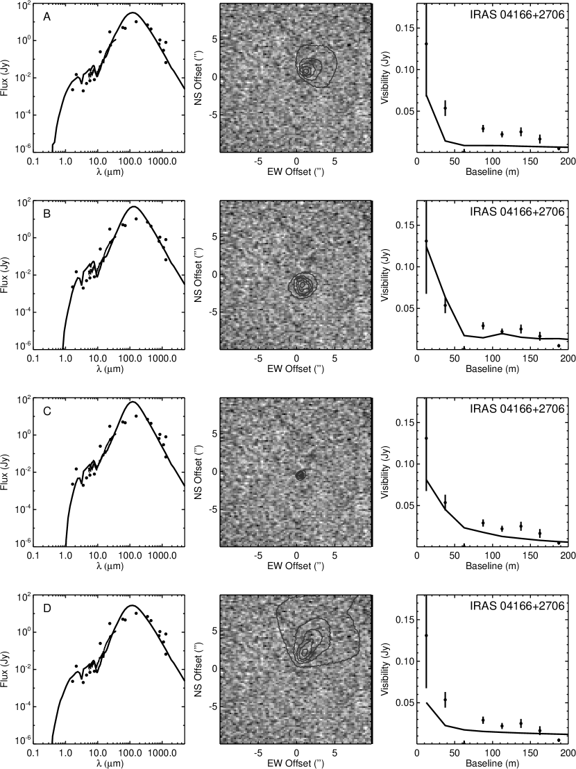
Figure 13: Observed and synthetic data for IRAS 04166+2706. See Figure 12 for a description of the various panels.

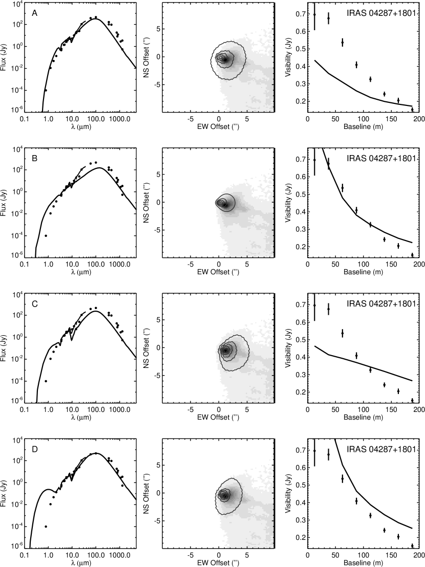
Figure 15: Observed and synthetic data for IRAS 04287+1801. See Figure 12 for a description of the various panels.

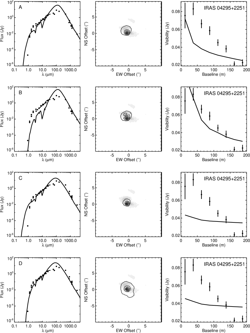
Figure 16: Observed and synthetic data for IRAS 04295+2251. See Figure 12 for a description of the various panels.

Table 4 lists the best fit model parameters for each object in our sample, and Figures 12–19 show observed and synthetic data for these models. For each object, we varied the relative weights of different datasets, to highlight the constraints imposed by each set of observations. Changing the relative weights allows us to explore the region around the $\chi^{2}$ minimum, and hence to determine how shallow the $\chi^{2}$ surface is when projected onto different parameters. For example, if a parameter is very well constrained then it will remain constant as data weights are varied. In contrast, some parameters may explore large values without significantly affecting fit quality.

In general, several parameters are well constrained, staying roughly constant as relative weights are varied. These include $M_{\rm disk}$, $L_{\ast}$, inclination, and position angle. This probably reflects the fact that these parameters tend to strongly influence one dataset, and to produce an effect that does not strongly resemble the effects of other model parameters. The main effect of $M_{\rm disk}$ is on the shape and strength of the millimeter visibilities (Figure 3). While $L_{\ast}$ does not directly translate into a flux normalization, its effects are mainly observed in the SED and the normalization of the millimeter visibilities. Since inclination and position angle produce strong, easily discernible effects on the synthetic scattered light images, their values can be constrained well.

In contrast, other parameters explore a wide range of values without significantly changing the overall fit quality. For example, $R_{\rm out}$ can vary over the entire range of explored values (from 500 to 2000 AU) in some cases. To some extent this reflects degeneracy among different parameters. As seen in Table 4, $M_{\rm env}$ varies in concert with $R_{\rm out}$. This is because larger $R_{\rm out}$ means that a given envelope mass is divided over a larger range of radii. As described in §3.2, other model parameters may also produce degenerate effects on various synthetic data.

The sparse sampling of our model grid occasionally leads to large apparent differences between models. In particular we only sample values of 1, 3, and 10 $L_{\odot}$ for $L_{\ast}$. Fitted values of 3 and 10 $L_{\odot}$ for a given source (e.g., IRAS 04016+2610; Table 4) do not necessarily indicate a factor of 3 uncertainty in the source luminosity. Rather, this probably reflects that the true source luminosity lies between these values. This point can be generalized to all parameters in our grid, which are sampled sparsely.

The main goals of our study are to constrain the disk mass, envelope mass, and their ratio. From Table 4, values for each of these can be extracted. We compute the average disk mass for each of the four best-fit models. The median disk mass for all the objects (using these averages) is 0.008 M_⊙. The median envelope mass is 0.08 M_⊙. For the overall sample, the envelope mass is $\sim 10$ times higher than the disk mass.

Another way to describe disk and envelope masses is to estimate the amount of mass on small scales relative to the more extended mass distribution. This circumvents uncertain interpretations of how much of the mass in our envelope model–which includes some material in a flattened, disk-like distribution within $R_{\rm c}$–should be counted as part to the disk mass.

In Figure 20 we plot the azimuthally-averaged mass distributions for all of the models listed in Table 4. It is evident that for most objects in our sample, the majority of the mass is found at larger radii. This is true even for the disk component, since the assumed surface density profile ($\Sigma\propto r^{-1.37}$) implies a radially increasing mass distribution. Moreover, Table 4 shows that envelope masses typically exceed disk masses in best-fit models.

Table 5 lists the total (disk+envelope) masses within 100 AU for each object and model. This scale corresponds roughly with the resolution of our $\lambda$1.3 mm observations. Constraints on the mass distribution on still more compact scales are uncertain. The mass found in the inner 100 AU has a median value of 0.007 M_⊙ for our sample (with large variations). The fractional contribution of this “compact” mass distribution to the total mass varies from 0.03 to 0.44, with a median value of 0.18.

Even though the mass within 100 AU is often a small fraction of the total mass, it produces a relatively large fraction of the millimeter flux (Figure 22). The circumstellar material is considerably hotter at small stellocentric radii. At long wavelengths where emission strength is approximately proportional to temperature and circumstellar mass, even a modest temperature gradient can lead to higher millimeter fluxes at smaller radii. Thus our modeling can constrain disk mass and geometry (as seen in Table 4) even if the disk contributes modestly to the total mass.

4.1 Comments on Individual Sources

4.1.1 IRAS 04016+2610

Models of this source generally fit all of the multi-wavelength data well. However, as seen in Figure 12, fitting the positional offset of the millimeter and I-band emission well leads to a somewhat worse fit to the SED data (third row of Figure 12 and Table 4). If we allow our modeled scattered light image to have a smaller offset than seen in the data, we can easily reproduce other aspects of the data. Furthermore, the offset in the model image is affected strongly by the outflow cavity parameter $\zeta$ (Figure 9), and so it seems that tweaking this parameter could improve the overall fits.

Our modeling of this source indicates a disk mass of 0.005 M_⊙, a disk radius of 250–450 AU, an envelope mass of 0.05–0.10 M_⊙, a luminosity of $\gtrsim 3$ $L_{\odot}$, an inclination of $\sim 35$–65^∘, and a PA of $\sim 60^{\circ}$. The disk scale height, outer radius, and envelope outflow cavity properties are less well constrained.

The envelope appears to be relatively massive around this source, with $\sim 10$ times more mass in the envelope than in the disk. The ratio of compactly distributed (within 100 AU) to the total mass is $\sim 0.03$ (Table 5). The large ratio of envelope to disk mass suggests a younger, less evolved object. On the other hand, the values of $R_{\rm disk}=R_{\rm c}$ are $\geq 250$ AU, comparable to disk sizes in T Tauri stars (e.g., Dutrey et al. 1996). Thus, the disk may be fully formed in this object, despite continuing infall from an extended envelope.

Earlier modeling of millimeter wavelength continuum and line data suggested a higher disk mass ($\sim 0.02$ M_⊙) with a more highly inclined (60–90^∘) viewing angle (Hogerheijde 2001). However more recent millimeter data has been interpreted in the context of a model including disk and envelope masses close to those derived here (Jørgensen et al. 2009). Analysis of scattered light images also produces geometric parameters consistent with those derived here (e.g., Gramajo et al. 2007). This well-studied object has even been subjected to previous modeling of combined multi-wavelength data (Eisner et al. 2005; Brinch et al. 2007a, b); again results of this modeling are consistent with those presented here. We note, finally, that the luminosity inferred in our modeling is compatible with the effective temperature of this source compared to other objects in our sample (Doppmann et al. 2005; Prato et al. 2009; Connelley & Greene 2010).

4.1.2 IRAS 04166+2706

For this object our models are able to reproduce well the observed SED and millimeter visibilities. Since no scattered light is detected from this source, the model scattered light image morphologies are not terribly important. However models with low scattered light fluxes are more consistent with the data. The models shown in the second and third rows of Figures 13 (and seen in the second and third entries for IRAS 04166+2706 in Table 4) have smaller optical/near-IR fluxes. These models still reproduce well the SED and millimeter visibilities.

Inferred disk masses for this object are $\sim 0.01$ M_⊙. While a heavy weighting of the scattered light imaging data produces a disk mass of 0, we note that this model has a much smaller value of $R_{\rm c}$ than others, which means that it still has a significant amount of compactly distributed mass. Indeed, the mass within 100 AU is 0.003–0.005 M_⊙ (Table 5) for all model fits to this object listed in Table 4.

The envelope mass is $\sim 0.10$ M_⊙, and the ratio of mass within 100 AU to the total is $\sim 0.05$. The large ratio of extended mass to compact mass suggests a young age. While the large inferred disk radius ($\sim 450$ AU) suggests a possible older age, we note that a similar fit can be achieved with no disk at all, but with an envelope including a flattened density distribution within $R_{\rm c}=30$ AU.

The luminosity for this object is inferred to be $\sim 1$–3 L_⊙. The inclination and position angle are 50-65^∘, and 120–240^∘, respectively. The large range in allowed inclination and position angle (compared with some other objects in our sample) is due to the lack of scattered light emission, which provides strong constraints on geometry. The disk scale height and envelope outer radius are not well constrained.

The results presented here are generally compatible with previous models of spectral energy distributions (e.g., Kenyon et al. 1993a; Furlan et al. 2008). However, our study is the first to model multi-wavelength images and the SED simultaneously.

4.1.3 IRAS 04169+2702

Our models for this source provide a reasonable fit to all of the data, although we deem the fits to be worse when we weight the scattered light imaging or SED data heavily. In these cases, models tend to under-predict the observed millimeter visibilities. However, as seen in the second row of Figure 14, additional weighting of the millimeter data leads to a model that fits all datasets well.

The scattered light images show no detectable emission, and the weak I-band flux in our models in compatible with this observation. The scattered light morphology in our models is also consistent with weak scattered light emission seen in previous work (e.g., Kenyon et al. 1993b).

The best-fit models, listed in Table 4, yield a disk mass of $\sim 0.01$ M_⊙, a disk radius of $\sim 250$–450 AU, and an envelope mass of $\sim 0.1$ M_⊙. The mass within 100 AU is $\sim 0.004$ M_⊙, which accounts for $\sim 0.04$ of the total mass (Table 5). The inferred luminosity is $\sim 1$ L_⊙, and the inclination and position angle are 30–35^∘ and 90^∘, respectively. As for other objects in our sample, the disk scale height, envelope outer radius, and outflow cavity filling factor, are not well-constrained.

4.1.4 IRAS 04287+1801 (L1551 IRS 5)

As seen in Figure 15, we were not able to provide a perfect fit to our entire multi-wavelength dataset. We can fit the SED and scattered light image well together, but that model under-predicts the millimeter visibilities (top row of Figure 15). If we fit the scattered light image and millimeter visibilities well, the SED fit quality is degraded (second row of Figure 15). We can fit all of the data reasonably well if we allow the model to over-predict the optical/near-IR fluxes (bottom row of Figure 15). Some additional extinction, for example from a different shape of the outflow cavity (Figure 9), may provide an even better fit.

The difficulty in achieving a high-quality fit to this object is due, in part, to the sparse sampling of parameter values in our modeling. Best-fit models often choose the highest sampled values of $M_{\rm disk}$, $M_{\rm env}$, and $L_{\ast}$. In particular, a value of $L_{\ast}>10L_{\odot}$ would produce a higher peak SED and larger overall millimeter visibilities (Figure 10). Thus, a luminosity larger than 10 $L_{\odot}$ would probably result in a better fit to the data.

IRAS 04287+1801 is also known to be a multiple system, which may complicate fitting of our simple models to the data. This object is clearly resolved as a $\sim 0\hbox to0.0pt{.\hss}^{\prime\prime}3$ binary (Rodriguez et al. 1998), and even shows evidence for a third component $<0\hbox to0.0pt{.\hss}^{\prime\prime}1$ away from the northern component in high resolution observations (Lim & Takakuwa 2006). All of these components would be within the resolution of our CARMA observations.

Previous authors have modeled SED data, scattered light imaging, and even millimeter imaging data for this source. Osorio et al. (2003) attempted to fit the SED and low-resolution sub-millimeter imaging with a binary protostar model. Their model specifies a circumbinary disk mass of 0.4 M_⊙, a disk radius of 300 AU, an envelope mass of $\sim 1$ M_⊙, $L_{\ast}=25$ L_⊙, and $i$=50^∘. Subsequent modeling of the SED (Furlan et al. 2008) or scattered light imaging (Gramajo et al. 2007) finds similar results, but with smaller envelope masses and disk/centrifugal radii.

Inferred parameter values from our modeling are: $M_{\rm disk}=0.1$–0.5 M_⊙, $R_{\rm disk}=100$–450 AU, $M_{\rm env}=0.05$–0.1 M_⊙, $L_{\ast}\sim 10$ L_⊙, $i=40$–50^∘, and PA=160–180^∘ (Table 4). These are generally consistent with previous results, with the exception of a lower $L_{\ast}$. It seems that we recover most of the details of the circumstellar mass distribution, even for this complicated multiple system, using relatively simple disk+envelope models.

4.1.5 IRAS 04295+2251

Best-fit models provide a reasonable fit to the combined dataset for IRAS 04295+2251, although better fits to individual datasets are possible at the expense of degrading the fits to other data (Figure 16). For example, the best-fit model to the millimeter visibility data does not fit the SED as well as other models. This may reflect the sparse sampling in our model grid to some extent. However, the fact that none of our models provide an excellent fit to the SED suggests that certain assumed parameters (e.g., dust opacities or outflow cavity shape) need to be adjusted to improve the overall fits.

Our modeling implies a disk mass of 0.01 M_⊙ and a relatively compact disk radius of 30–100 AU. The envelope mass is inferred to be 0.005-0.05 M_⊙, the envelope radius is 500–1000 AU, $L_{\ast}=1L_{\odot}$, and the inclination and position angle are 45–55^∘ and 300^∘, respectively (Table 4). This source has a high fraction of compact-to-extended mass, with $\sim 44\%$ of the matter distributed within 100 AU (Table 5).

While most of the inferred parameter values are similar to those found in previous modeling of multi-wavelength data (Eisner et al. 2005), the disk mass presented here is substantially lower. We find 0.01 M_⊙, while Eisner et al. (2005) found 1 M_⊙. However, Eisner et al. (2005) assumed the disk mass was distributed over radii out to 500 AU, while the modeling presented here places the disk mass within 30–100 AU. Given the higher resolution of the data presented here, it is not surprising that the disk mass is now constrained to smaller radii. Since the matter at smaller radii produces most of the emission (Figure 22), a smaller disk requires less total mass to reproduce the observations.

4.1.6 IRAS 04302+2247

We are unable to find a single model that reproduces the combined multi-wavelength dataset for this source. We can fit well the SED and millimeter data together, or the SED and scattered light data together, but not the millimeter and scattered light data together (Figure 17). However, the best-fit models for different data weightings produce fairly consistent values for some parameters. Disk mass is 0.005–0.01 M_⊙, and the disk radius is 100–250 AU. The envelope mass is not well constrained, spanning values between 0.005 and 0.1 M_⊙, while the envelope outer radius appears to be $\sim 500$ AU. The inclination is 70–89^∘, and the PA is 10^∘. The mass within 100 AU is found to be $\sim 0.006$ M_⊙, accounting for $\sim 20\%$ of the total mass (Table 5).

Previous modeling of millimeter and scattered light imaging data argued for different dust grain properties in the disk and envelope components (Wolf et al. 2003). We have not included such effects in our modeling, which may explain why we have difficulty fitting the millimeter visiblities and the scattered light images simultaneously. With a detailed model for this single object, Wolf et al. (2003) derived $M_{\rm disk}=0.07$ AU, $R_{\rm disk}=300$ AU, $h_{\rm 1\>AU}=0.15$ AU, $M_{\rm env}=0.05$ M_⊙, and $R_{\rm out}=450$ AU. For the most part, our modeling (Table 4) is consistent with these results. The disk mass we infer is substantially lower, however, perhaps due to a somewhat smaller fitted disk radius, as well as different assumed opacities.

4.1.7 IRAS 04361+2547

We are able to fit the data for this source quite well, especially when the imaging data is given some additional weight compared to the SED data (Figure 18). The disk mass is inferred to be 0.005–0.01 M_⊙, and the envelope mass is comparable, $\sim 0.01$ M_⊙. The disk radius is not well constrained, while the outer radius of the envelope is inferred to be 500 AU. The total luminosity is 3 $L_{\odot}$, the inclination is $\sim 45^{\circ}$, and the position angle is $\sim 280^{\circ}$. This source exhibits a relatively high fraction of compact-to-extended mass content, with $\sim 40\%$ of the mass distributed within 100 AU (Table 5).

The disk mass we derive is consistent with Jørgensen et al. (2009, who found $M_{\rm disk}=0.009$ M_⊙), but the envelope mass we infer here is somewhat lower. This is probably a consequence of the fact that our millimeter observations are not sensitive to emission more extended than $\sim 1000$ AU, while Jørgensen et al. (2009) used single-dish observations to detect more extended emission. We predict a somewhat lower inclination than found in previous scattered light imaging (Kenyon et al. 1993b; Gramajo et al. 2007); however yet lower inclination is inferred in previous SED modeling (Kenyon et al. 1993a). Thus our inferred geometry is generally consistent with previous work.

4.1.8 IRAS 04365+2535

Our models for IRAS 04365+2535 fit the combined multi-wavelength dataset well, regardless of data weighting factors (Figure 19). Best-fit models imply $M_{\rm disk}=0.005$ M_⊙, $R_{\rm disk}=100$ AU, $M_{\rm env}=0.05$–0.1 M_⊙, $R_{\rm out}=500$–1000 AU, $L_{\ast}=1$ $L_{\odot}$, inclination$=25^{\circ}$, and position angle$=310^{\circ}$. The mass enclosed within 100 AU is $\sim 0.007$ M_⊙, which comprises $\sim 11\%$ of the total mass.

Previous analysis of millimeter visibility data determined a disk mass of 0.03 M_⊙ and an envelope mass of 0.12 M_⊙ (Jørgensen et al. 2009). The disk mass in particular is higher than we infer in our analysis. This discrepancy is probably due to the lower angular resolution in the previous observations: $\sim 2\hbox to0.0pt{.\hss}^{\prime\prime}5=350$ AU. In contrast, we infer a disk size of 100 AU. With a larger beam, the earlier observations could have easily inferred a larger mass. The results of our modeling also appear consistent with previous modeling of the SED or scattered light imaging (Kenyon et al. 1993a, b; Gramajo et al. 2007), although our inferred inclination is somewhat lower than previous estimates.

5 Discussion

The disk mass is a crucial parameter in understanding both star and planet formation. High disk masses, on the order of a tenth of the stellar mass, would imply that gravitational instability may be important. Such instability can lead to rapid accretion onto the central protostar, and may explain why accretion rates onto the star appear low compared to estimated time-averaged accretion from the envelope onto the disk. Episodes of gravitationally-enhanced accretion can lead to larger time-averaged rates but low typical instantaneous accretion rates (e.g., White & Hillenbrand 2004; Eisner et al. 2005).

Disk mass is also a critical initial condition for planet formation. To form gas giants like Jupiter and Saturn requires $>0.01$ M_⊙ of matter (Weidenschilling 1977b). While measured disk masses around T Tauri stars are smaller (e.g., Andrews & Williams 2005; Eisner et al. 2008), this may reflect the agglomeration of small particles into larger bodies rather than a mass deficit. Data for the less evolved protostars in our sample can provide masses in systems where dust grain agglomeration is presumably less advanced.

We begin by examining the distribution of disk masses for our sample, drawing values from Table 4. Disk masses range from 0.005 to 0.5 M_⊙ across the sample, and the median disk mass is 0.008 M_⊙. The majority ($\sim 60\%$) of objects have disk masses $\geq 0.01$ M_⊙, and $\sim 10\%$ have $M_{\rm disk}\geq 0.1$ M_⊙. For comparison, across $>150$ (more evolved) Class II disks in Taurus, Andrews & Williams (2005) find a median mass of 0.005 M_⊙. In this sample of Class II objects, $\sim 20\%$ of disks are more massive than 0.01 M_⊙ and only $\sim 2\%$ are more massive than 0.1 M_⊙ (Andrews & Williams 2005).

Our sample of Taurus Class I objects has significantly more massive disks than the Class II population. Indeed, many of them may still possess sufficient mass in small ($\sim$mm-sized) dust grains for the eventual formation of planetary systems like our own (depending on how the mass is distributed on scales smaller than 100 AU). The lower masses in Class II disks likely reflect that some of the mass of small particles available at the Class I stage has grown into large ($>$ meter-sized) bodies within $\sim 1$ Myr.

This argument can easily be extended to Class I sources themselves. While Class I disks appear more massive than Class II disks—at least as traced by small ($\lesssim$ mm-sized) dust grains—particles in Class I disks may already have undergone substantial processing. That is, planet formation may already be underway even at these ages. Extending the analysis in this paper to younger, less evolved Class 0 objects provides a clear path to improving the estimates of the initial mass content of protoplanetary disks.

The range of disk masses observed for our sample indicates that few Class I disks are at the limit of gravitational instability. Even IRAS 04287+1801, which has a disk mass $\geq 0.1$ M_⊙, may remain stable against gravitational collapse because of the higher stellar mass contained in the multiple central system. If, however, substantial mass is hidden in larger bodies, gravitational instability may still be possible in these systems.

Measured envelope masses can be used to estimate the mass infall rate from the envelope onto the disk, $\dot{M}$. Estimates of $\dot{M}$ can then be compared to the accretion rate measured from the inner disk onto the star (e.g., White & Hillenbrand 2004). Such comparisons typically conclude that the infall rate from the envelope is higher than the accretion rate onto the star, suggesting that matter piles up in the disk and periodically accretes quickly in bursts (e.g., Kenyon & Hartmann 1987; White & Hillenbrand 2004; Eisner et al. 2005; Vorobyov & Basu 2005). The results presented here are generally compatible with this view.

However the envelope masses estimated here are highly uncertain. For example, the range of $M_{\rm env}$ allowed for IRAS 04016+2610 (Table 4) correspond to $\dot{M}$ between $\sim 10^{-6}$ and $10^{-5}$ M_⊙ yr^-1. Much of this uncertainty is due to degeneracies with other parameters (primarily $R_{\rm out}$; see §3.2). Additional uncertainties arise because of the limited $uv$ coverage (i.e., range of telescope baseline separations) in our millimeter observations. The shortest baselines correspond to linear resolutions of $\sim 1000$ AU at the distance to our targets. More extended emission is largely resolved out. Thus, we are not sensitive to extended emission and, as a result, our total envelope masses are likely underestimated.

Despite uncertainties in inferred values of $M_{\rm env}$, clear differences in the ratio of $M_{\rm disk}/M_{\rm env}$ are observed across our sample. The disk-to-envelope mass ratio ranges from $<0.1$ for some objects (IRAS 04016+2610) to $>1$ for others (IRAS 04287+1801). In most cases, the disk-to-envelope mass ratio is around 0.1. This suggests our sample is at an earlier evolutionary stage than Class II objects, which are essentially 100% disk. Furthermore, one might be tempted to assign relative ages to sample objects based on $M_{\rm disk}/M_{\rm env}$ values.

Another method to constrain relative ages in our sample is to examine the disk/centrifugal radii. For collapsing, rotating envelopes, the centrifugal radius grows with time because of the inside-out nature of the collapse. For the envelope models used here, one expects the centrifugal, and hence disk, radius to grow with time as $R(t)\propto t^{3}$. If our sample objects had similar initial specific angular momenta (which is by no means guaranteed), then the inferred centrifugal radii can be used to estimate relative ages.

The disk radii inferred in our modeling have substantial uncertainties, but do reveal trends between objects (Table 4). For example, IRAS 04016+2610 seems to have a larger disk/centrifugal radius than IRAS 04295+2251. However, IRAS 04016+2610 has a lower disk-to-envelope mass ratio than IRAS 04295+2251. While a smaller disk/centrifugal radius suggests a younger source, a larger ratio of disk-to-envelope mass suggests an older object. We therefore do not place much confidence in our ability to distinguish ages amongst our sample.

To compare our inferred disk masses with expected minimum masses for planet formation theory, we turn now to the masses listed in Table 5. The Table lists circumstellar masses enclosed within 100 AU, including both disk and inner envelope components. Since the inner regions of the envelope have a flattened density distribution (Equation 1), they may appear disk-like, and may contribute to the mass budget for planet formation.

We choose 100 AU because this is approximately the smallest scale we can resolve with our millimeter imaging data. However we would ideally like to probe smaller scales, since planet formation theories usually require a minimum mass within radii or 30–50 AU (e.g., Weidenschilling 1977b; Hayashi 1981). Thus, even our 100-AU-masses (Table 5) may over-estimate the mass available for planet formation. Even so, the masses listed in Table 5 are typically lower than the 0.01–0.1 M_⊙ usually required to form planetary systems like ours. As discussed above, this may reflect growth of small, observable dust grains into larger bodies. Probing younger sources may provide a clearer picture of how much mass is truly available to planet formation.

6 Summary and Future Directions

We described new millimeter imaging observations of a sample of Class I protostars, obtained with the CARMA interferometer. We presented basic properties of the millimeter emission, and a more detailed analysis of the millimeter data in conjunction with imaging and flux data at other wavelengths. We constructed models consisting of rotating, infalling envelopes and embedded, compact disks, and generated a grid of synthetic multi-wavelength datasets using the radiative transfer code RADMC. We fitted these models to the multi-wavelength dataset for each target.

Our focus in this study is measuring disk and envelope masses. We found disk masses for our sample ranging from $\lesssim 0.01$ to $\gtrsim 0.1$ M_⊙. The compact disks typically only comprise a small percentage of the total mass ($\lesssim 10\%$), although this percentage is higher in a few objects. Envelope masses—and by extension, the disk-to-envelope mass ratios—are usually poorly constrained by our modeling. This is due, in large part, to the limited sensitivity of our observations to emission more extended than $\sim 1000$ AU. Better $uv$ coverage, for example combining extended and compact configurations of CARMA or ALMA, will alleviate this problem in the future.

The disk masses inferred for our sample are significantly higher than for samples of more evolved Class II objects. Thus, Class I disk masses probably provide a more accurate estimate of the initial mass budget for star and planet formation, before particle growth and planetesimal formation lock up mass in hard-to-see larger bodies. However, such particle agglomeration may already be underway by the Class I epoch, and so measured disk masses may still be underestimates. Observing Class I sources at multiple millimeter and sub-millimeter wavelengths with ALMA will help to constrain grain properties and how these depend on location in the disk, providing tighter constraints on disk masses and the extent of grain growth.

Another obvious extension of this project is to observe larger samples of protostars over a range of evolutionary states. In particular, observations and modeling of Class 0 protostars can reveal if their disk masses are larger than those inferred around Class I objects. Comparing disk masses for samples of objects at different ages will constrain how the mass in small dust grains evolves, and give a better estimate of the true initial disk mass distribution.

The angular resolution of our observations is sufficient to constrain the disk mass distribution within $\sim 100$ AU. In contrast, planet formation models generally only consider the mass within 30–50 AU. Future work, using more extended array configurations of CARMA or ALMA, can reach these scales and provide constraints on disk masses that are directly comparable to critical initial conditions of planet formation theories.

Figure 2: Averaged visibility amplitudes for our targets. Visibilities computed on a two-dimensional grid are shown with open circles. The error bars on these points are typically fairly large (often comparable to the plotted range) and are not shown here. We also plot the azimuthally averaged visibilities with solid points. The additional averaging leads to substantially smaller uncertainties, indicated here with plotted error bars. Note that the averaging is done coherently, and phase noise may lead to average amplitudes below the amplitudes measured for unaveraged data.

Figure 3: Fluxes (top left), normalized $\lambda$1.3mm visibility profiles (top right), and 0.9 $\micron$ images (bottom) for disk+envelope models with different disk masses. Contours are plotted for 10%, 30%, 50%, 70%, and 90% of the peak flux levels. As listed in §3.2, all models have $M_{\rm env}=0.05$ M_⊙, $\alpha=-2.37$, $h_{\rm 1\>AU}=0.05$ AU, $R_{\rm disk}=R_{\rm c}=30$ AU, $R_{\rm out}=1000$ AU, $f_{\rm cav}=0.2$, $\zeta=1.0$, $L_{\ast}=3$ L_⊙, $i=45^{\circ}$, and position angle $=90^{\circ}$.

Figure 4: Fluxes (top left), normalized $\lambda$1.3mm visibility profiles (top right), and 0.9 $\micron$ images (bottom) for disk+envelope models with different disk scale heights. Contours are plotted for 10%, 30%, 50%, 70%, and 90% of the peak flux levels. Parameters of the basic model are listed in §3.2 and in the caption of Figure 3.

Figure 5: Fluxes (top left), normalized $\lambda$1.3mm visibility profiles (top right), and 0.9 $\micron$ images (bottom) for disk+envelope models with different disk/centrifugal radii. Contours are plotted for 10%, 30%, 50%, 70%, and 90% of the peak flux levels. Parameters of the basic model are listed in §3.2 and in the caption of Figure 3.

Figure 6: Fluxes (top left), normalized $\lambda$1.3mm visibility profiles (top right), and 0.9 $\micron$ images (bottom) for disk+envelope models with different envelope masses. Contours are plotted for 10%, 30%, 50%, 70%, and 90% of the peak flux levels. Parameters of the basic model are listed in §3.2 and in the caption of Figure 3.

Figure 7: Fluxes (top left), normalized $\lambda$1.3mm visibility profiles (top right), and 0.9 $\micron$ images (bottom) for disk+envelope models with different envelope outer radii. Contours are plotted for 10%, 30%, 50%, 70%, and 90% of the peak flux levels. Parameters of the basic model are listed in §3.2 and in the caption of Figure 3.

Figure 8: Fluxes (top left), normalized $\lambda$1.3mm visibility profiles (top right), and 0.9 $\micron$ images (bottom) for disk+envelope models with different density contrasts within the outflow cavity. Contours are plotted for 10%, 30%, 50%, 70%, and 90% of the peak flux levels. Parameters of the basic model are listed in §3.2 and in the caption of Figure 3.

Figure 9: Fluxes (top left), normalized $\lambda$1.3mm visibility profiles (top right), and 0.9 $\micron$ images (bottom) for disk+envelope models with different outflow cavity shapes. Contours are plotted for 10%, 30%, 50%, 70%, and 90% of the peak flux levels. Parameters of the basic model are listed in §3.2 and in the caption of Figure 3.

Figure 10: Fluxes (top left), normalized $\lambda$1.3mm visibility profiles (top right), and 0.9 $\micron$ images (bottom) for disk+envelope models with different source luminosities. Contours are plotted for 10%, 30%, 50%, 70%, and 90% of the peak flux levels. Parameters of the basic model are listed in §3.2 and in the caption of Figure 3.

Figure 11: Fluxes (top left), normalized $\lambda$1.3mm visibility profiles (top right), and 0.9 $\micron$ images (bottom) for disk+envelope models with different viewing geometries. Contours are plotted for 10%, 30%, 50%, 70%, and 90% of the peak flux levels. Parameters of the basic model are listed in §3.2 and in the caption of Figure 3.

Figure 12: Observed and synthetic data for IRAS 04016+2610. We plot: broadband SEDs, including Spitzer/IRS spectra (left panels); I-band scattered light images (middle panels); and azimuthally-averaged $\lambda$1.3mm visibilities (right panels). Models are represented by solid curves in the left and right panels, and by contours in the middle panels. The different rows show best-fit models for different relative weightings of the datasets. The plotted models follow the same ordering (top-to-bottom) as the entries in Table 4, where data weights and parameters of best-fit models are listed.

Figure 14: Observed and synthetic data for IRAS 04169+2702. See Figure 12 for a description of the various panels.

Figure 17: Observed and synthetic data for IRAS 04302+2247. See Figure 12 for a description of the various panels.

Figure 18: Observed and synthetic data for IRAS 04361+2547. See Figure 12 for a description of the various panels.

Figure 19: Observed and synthetic data for IRAS 04365+2535. See Figure 12 for a description of the various panels.

Figure 20: Radial mass distributions for all the models listed in Table 4. We show the mass distributions for the disk components (dotted curves), the envelope components (dashed curves), and the total disk+envelope models (solid curves). Each row show the mass profiles for model fits to a single object, with the ordering of columns (left-to-right) corresponding to the ordering of rows (top-to-bottom) in Table 4.

Figure 21: Figure 20 continued.

Figure 22: Radial mass distribution (left) and azimuthally averaged $\lambda$1.3 mm flux distribution (right) for the disk+envelope model listed in the first row (model “A” for IRAS 04016+2610) of Table 4. The disk component contributes most of the mass within 100 AU, although this represents only a small percentage of the total mass. However the disk component dominates the observed flux at $\lambda$1.3 mm, at least on the relatively compact scales ($\lesssim 1000$ AU) probed by our CARMA observations. Note that the component fluxes were determined from models where the disk or envelope mass was set to zero, while the flux of the disk+envelope model is determined from radiative transfer modeling for the combined density distribution.

Table 1: Log of Observations

Source	Observation Date	Baselines	Passband Calibrators	Gain Calibrator
	(UT)	(m)
IRAS 04016+2610	2008 Oct 18, 22; 2008 Nov 17	18–199	3C84, 3C454.3	3C111
IRAS 04166+2706	2010 Oct 27	20-251	3C279, 3C273	3C111
IRAS 04169+2702	2010 Oct 27	20-250	3C279, 3C273	3C111
IRAS 04181+2654	2010 Oct 27	20-250	3C279, 3C273	3C111
IRAS 04263+2426	2010 Oct 29	19-251	3C84, 3C111	3C111
IRAS 04287+1801	2008 Oct 21, 22	18–197	3C84, 3C454.3	3C111
IRAS 04295+2251	2008 Oct 18, 22; 2008 Nov 17	17–198	3C84, 3C454.3	3C111
IRAS 04302+2247	2008 Oct 21, 22	18–199	3C84, 3C454.3	3C111
IRAS 04361+2547	2010 Oct 29	19-251	3C84, 3C111	3C111
IRAS 04365+2535	2010 Oct 29	19-232	3C84, 3C111	3C111

Table 2: Properties of 1.3-mm wavelength images

Source	$\alpha$	$\delta$	Peak Flux	RMS	$\theta_{\rm maj}$	$\theta_{\rm min}$	$\theta_{\rm PA}$
	(J2000)	(J2000)	(mJy)	(mJy)	(′′)	(′′)	(∘)
IRAS 04016+2610	04:04:43.07	+26:18:56.3	17	1	1.13	0.85	54.
IRAS 04166+2706	04:19:42.50	+27:13:36.0	66	13	1.03	0.90	74.0
IRAS 04169+2702	04:19:58.48	+27:09:57.0	65	8	1.02	0.90	75.9
IRAS 04181+2654	…	…	…	5	1.03	0.90	75.4
IRAS 04263+2426N	04:29:23.72	+24:33:01.0	37	4	1.02	0.85	-72.5
IRAS 04263+2426S	04:29:23.74	+24:32:59.8	31	4	1.02	0.85	-72.5
IRAS 04287+1801	04:31:34.16	+18:08:04.8	404	4	1.09	0.86	44.9
IRAS 04295+2251	04:32:32.07	+22:57:26.3	53	1	1.13	0.86	53.5
IRAS 04302+2247	04:33:16.49	+22:53:20.3	46	2	1.07	0.86	49.3
IRAS 04361+2547	04:39:13.90	+25:53:20.44	50	4	1.03	0.84	-69.7
IRAS 04365+2535	04:39:35.21	+25:41:44.2	147	5	1.04	0.83	-68.6

Note. — Coordinates indicate the positions of the peak fluxes. The major axis, minor axis, and position angle (east-of-north) of the beam FWHM are listed as $\theta_{\rm maj}$, $\theta_{\rm min}$, and $\theta_{\rm PA}$, respectively.

Table 3: Uniform Disk Model Fits to CARMA Visibility Amplitudes

Source	Flux	$\theta_{\rm UD}$	$i$	PA
	(mJy)	(′′)	(∘)	(∘)
IRAS 04016+2610	$18\pm 2$	$2.49\pm 0.19$	$68\pm 7$	$66\pm 4$
IRAS 04166+2706	$36\pm 8$	$0.75\pm 1.00$	$90\pm 90$	$130\pm 130$
IRAS 04169+2702	$71\pm 16$	$1.30\pm 0.64$	$50\pm 50$	$0\pm 180$
IRAS 04287+1801	$536\pm 35$	$1.61\pm 0.07$	$55\pm 9$	$167\pm 6$
IRAS 04295+2251	$78\pm 8$	$2.05\pm 0.12$	$60\pm 7$	$73\pm 7$
IRAS 04302+2247	$29\pm 15$	$2.76\pm 1.26$	$67\pm 22$	$33\pm 20$
IRAS 04361+2547	$62\pm 28$	$1.76\pm 0.84$	$60\pm 60$	$160\pm 160$
IRAS 04365+2535	$110\pm 48$	$2.14\pm 0.72$	$89\pm 44$	$84\pm 25$

Note. — For each source, we list the flux, angular diameter ($\theta_{\rm UD}$), inclination, and position angle for best-fit inclined uniform disk models.

Table 4: Best-fit Disk+Envelope Models

Source		$w_{mm}$	$w_{\rm Iband}$	$w_{\rm SED}$	$\chi_{r}^{2}$	$M_{\rm disk}$	$R_{\rm disk}$	$h_{\rm 1AU}$	$M_{\rm env}$	$R_{\rm out}$	$f_{\rm cav}$	$L_{\ast}$	$i$	PA
					(M⊙)	(AU)	(AU)	(M⊙)	(AU)		(L⊙)	(∘)	(∘)
IRAS 04016+2610	A	1	1	1	5.0	0.005	250	0.05	0.10	2000	1	3	35	60
IRAS 04016+2610	B	10	1	1	3.0	0.005	250	0.05	0.10	2000	1	3	40	60
IRAS 04016+2610	C	1	10	1	3.9	0.005	450	0.05	0.05	1000	0.2	10	65	60
IRAS 04016+2610	D	1	1	10	2.8	0.005	450	0.15	0.05	500	0.2	3	35	60
IRAS 04166+2706	A	1	1	1	1.6	0.01	450	0.15	0.10	1000	0.2	1	55	210
IRAS 04166+2706	B	10	1	1	1.4	0.01	450	0.05	0.10	500	0.2	1	50	120
IRAS 04166+2706	C	1	10	1	1.2	0.0	30	…	0.05	500	0.02	3	60	140
IRAS 04166+2706	D	1	1	10	1.9	0.01	450	0.15	0.10	2000	0.2	1	65	240
IRAS 04169+2702	A	1	1	1	2.1	0.01	450	0.15	0.10	2000	1	1	30	90
IRAS 04169+2702	B	10	1	1	1.6	0.01	250	0.05	0.10	500	0.2	1	35	90
IRAS 04169+2702	C	1	10	1	1.4	0.01	450	0.15	0.10	2000	1	1	30	90
IRAS 04169+2702	D	1	1	10	2.4	0.0	100	…	0.05	500	0.02	1	55	90
IRAS 04287+1801	A	0.1	1	1	6.6	0.10	250	0.05	0.05	1000	1	10	40	160
IRAS 04287+1801	B	0.5	1	1	8.1	0.50	450	0.05	0.10	1000	0.2	3	40	180
IRAS 04287+1801	C	0.1	10	1	2.8	0.10	100	0.05	0.10	2000	0.2	10	50	160
IRAS 04287+1801∗	D	1	1	10	9.0	0.50	450	0.05	0.01	2000	0.2	10	50	160
IRAS 04295+2251	A	1	1	1	3.3	0.01	100	0.05	0.05	1000	0.2	1	45	300
IRAS 04295+2251	B	10	1	1	2.2	0.01	100	0.05	0.05	500	0.2	1	45	300
IRAS 04295+2251	C	1	10	1	1.9	0.01	30	0.05	0.005	500	0.2	1	50	300
IRAS 04295+2251	D	1	1	10	1.9	0.01	30	0.05	0.005	500	1	1	55	300
IRAS 04302+2247	A	1	1	1	3.8	0.01	250	0.05	0.05	500	0.2	1	70	10
IRAS 04302+2247	B	10	1	1	3.0	0.01	250	0.05	0.10	500	0.2	1	75	10
IRAS 04302+2247	C	1	10	1	2.2	0.005	100	0.15	0.005	500	1	1	89	10
IRAS 04302+2247	D	1	1	10	3.7	0.01	250	0.15	0.05	2000	0.2	1	70	10
IRAS 04361+2547	A	1	1	1	4.8	0.005	30	0.15	0.005	500	1	3	55	310
IRAS 04361+2547	B	10	1	1	2.6	0.01	450	0.15	0.01	500	1	3	45	280
IRAS 04361+2547	C	1	10	1	2.1	0.005	100	0.15	0.01	500	1	3	45	280
IRAS 04361+2547	D	1	1	10	5.5	0.005	30	0.15	0.005	500	1	3	55	310
IRAS 04365+2535	A	1	1	1	1.3	0.005	100	0.05	0.05	500	0.2	1	25	310
IRAS 04365+2535	B	10	1	1	1.3	0.005	100	0.15	0.10	1000	1	1	25	310
IRAS 04365+2535	C	1	10	1	1.1	0.005	100	0.05	0.05	500	0.2	1	25	310
IRAS 04365+2535	D	1	1	10	1.5	0.005	100	0.05	0.05	500	0.2	1	25	310

Note. — The reduced $\chi^{2}$ is defined by Equation 10. For each source, the first row represents our best attempt at providing equal weights to each dataset. The following three rows show the best-fit models when one dataset is weighted up relative to the others. We label each row A,B,C, or D. In some cases, the best-fit model is the same for different weights, although the reduced $\chi^{2}$ values may differ. Note that $R_{\rm disk}=R_{\rm c}$, and so this column is meaningful even when $M_{\rm disk}=0$.

^∗—for this model we increased the weight of the IRS data relative to the remaining SED data. With normal weighting of the IRS data, the SED-weighted data is fit best with the first model listed for this object.

Table 5: Model Mass Distributions

Source	Mass within 100 AU					Mass within 100 AU
	(M⊙)					/ Total Mass
	A	B	C	D	Mean
IRAS 04016+2610	0.003	0.003	0.002	0.002	$0.002\pm 0.0004$	$0.03\pm 0.008$
IRAS 04166+2706	0.003	0.005	0.005	0.003	$0.004\pm 0.0009$	$0.05\pm 0.03$
IRAS 04169+2702	0.003	0.007	0.003	0.002	$0.004\pm 0.002$	$0.04\pm 0.01$
IRAS 04287+1801	0.05	0.18	0.09	0.18	$0.12\pm 0.06$	$0.37\pm 0.07$
IRAS 04295+2251	0.01	0.01	0.01	0.01	0.01 $\pm$ 0.0008	$0.44\pm 0.30$
IRAS 04302+2247	0.006	0.007	0.005	0.005	$0.006\pm 0.001$	$0.18\pm 0.18$
IRAS 04361+2547	0.005	0.003	0.005	0.005	$0.005\pm 0.0008$	$0.40\pm 0.17$
IRAS 04365+2535	0.007	0.006	0.007	0.007	$0.007\pm 0.0007$	$0.11\pm 0.04$

Note. — For each source, we list the mass within 100 AU for the four models listed in Table 4. We then give the mean value and the standard deviation. Finally, we list the fractional mass within 100 AU compared to the total mass.

References

- Adams et al. (1987) Adams, F. C., Lada, C. J., & Shu, F. H. 1987, ApJ, 312, 788
- André et al. (1993) André, P., Ward-Thompson, D., & Barsony, M. 1993, ApJ, 406, 122
- Andrews & Williams (2005) Andrews, S. M., & Williams, J. P. 2005, ApJ, 631, 1134
- Andrews & Williams (2007) —. 2007, ApJ, 671, 1800
- Barsony & Kenyon (1992) Barsony, M., & Kenyon, S. J. 1992, ApJ, 384, L53
- Basri & Bertout (1989) Basri, G., & Bertout, C. 1989, ApJ, 341, 340
- Brinch et al. (2007a) Brinch, C., Crapsi, A., Hogerheijde, M. R., & Jørgensen, J. K. 2007a, A&A, 461, 1037
- Brinch et al. (2007b) Brinch, C., Crapsi, A., Jørgensen, J. K., Hogerheijde, M. R., & Hill, T. 2007b, A&A, 475, 915
- Burrows et al. (1996) Burrows, C. J., Stapelfeldt, K. R., Watson, A. M., Krist, J. E., Ballester, G. E., Clarke, J. T., Crisp, D., Gallagher, J. S., Griffiths, R. E., Hester, J. J., Hoessel, J. G., Holtzman, J. A., Mould, J. R., Scowen, P. A., Trauger, J. T., & Westphal, J. A. 1996, ApJ, 473, 437
- Chandler & Richer (2000) Chandler, C. J., & Richer, J. S. 2000, ApJ, 530, 851
- Chiang & Goldreich (1997) Chiang, E. I., & Goldreich, P. 1997, ApJ, 490, 368
- Chiang & Goldreich (1999) —. 1999, ApJ, 519, 279
- Cieza et al. (2007) Cieza, L., Padgett, D. L., Stapelfeldt, K. R., Augereau, J.-C., Harvey, P., Evans, II, N. J., Merín, B., Koerner, D., Sargent, A., van Dishoeck, E. F., Allen, L., Blake, G., Brooke, T., Chapman, N., Huard, T., Lai, S.-P., Mundy, L., Myers, P. C., Spiesman, W., & Wahhaj, Z. 2007, ApJ, 667, 308
- Connelley & Greene (2010) Connelley, M. S., & Greene, T. P. 2010, AJ, 140, 1214
- Corder et al. (2005) Corder, S., Eisner, J., & Sargent, A. 2005, ApJ, 622, L133
- D’Alessio et al. (1999) D’Alessio, P., Calvet, N., Hartmann, L., Lizano, S., & Cantó, J. 1999, ApJ, 527, 893
- Doppmann et al. (2005) Doppmann, G. W., Greene, T. P., Covey, K. R., & Lada, C. J. 2005, AJ, 130, 1145
- Doppmann et al. (2008) Doppmann, G. W., Najita, J. R., & Carr, J. S. 2008, ApJ, 685, 298
- Dullemond & Dominik (2004) Dullemond, C. P., & Dominik, C. 2004, A&A, 417, 159
- Dutrey et al. (1996) Dutrey, A., Guilloteau, S., Duvert, G., Prato, L., Simon, M., Schuster, K., & Menard, F. 1996, A&A, 309, 493
- Eisner et al. (2005) Eisner, J. A., Hillenbrand, L. A., Carpenter, J. M., & Wolf, S. 2005, ApJ, 635, 396
- Eisner et al. (2004) Eisner, J. A., Lane, B. F., Hillenbrand, L., Akeson, R., & Sargent, A. 2004, ApJ, 613, 1049
- Eisner et al. (2008) Eisner, J. A., Plambeck, R. L., Carpenter, J. M., Corder, S. A., Qi, C., & Wilner, D. 2008, ApJ, 683, 304
- Enoch et al. (2009) Enoch, M. L., Evans, N. J., Sargent, A. I., & Glenn, J. 2009, ApJ, 692, 973
- Evans et al. (2009) Evans, N. J., Dunham, M. M., Jørgensen, J. K., Enoch, M. L., Merín, B., van Dishoeck, E. F., Alcalá, J. M., Myers, P. C., Stapelfeldt, K. R., Huard, T. L., Allen, L. E., Harvey, P. M., van Kempen, T., Blake, G. A., Koerner, D. W., Mundy, L. G., Padgett, D. L., & Sargent, A. I. 2009, ApJS, 181, 321
- Furlan et al. (2011) Furlan, E., Luhman, K. L., Espaillat, C., D’Alessio, P., Adame, L., Manoj, P., Kim, K. H., Watson, D. M., Forrest, W. J., McClure, M. K., Calvet, N., Sargent, B. A., Green, J. D., & Fischer, W. J. 2011, ApJS, 195, 3
- Furlan et al. (2008) Furlan, E., McClure, M., Calvet, N., Hartmann, L., D’Alessio, P., Forrest, W. J., Watson, D. M., Uchida, K. I., Sargent, B., Green, J. D., & Herter, T. L. 2008, ApJS, 176, 184
- Gramajo et al. (2007) Gramajo, L. V., Whitney, B. A., Kenyon, S. J., Gómez, M., & Merrill, K. M. 2007, AJ, 133, 1911
- Greene et al. (1994) Greene, T. P., Wilking, B. A., Andre, P., Young, E. T., & Lada, C. J. 1994, ApJ, 434, 614
- Hartigan et al. (1995) Hartigan, P., Edwards, S., & Ghandour, L. 1995, ApJ, 452, 736
- Hartmann et al. (1997) Hartmann, L., Cassen, P., & Kenyon, S. J. 1997, ApJ, 475, 770
- Hartmann et al. (2005) Hartmann, L., Megeath, S. T., Allen, L., Luhman, K., Calvet, N., D’Alessio, P., Franco-Hernandez, R., & Fazio, G. 2005, ApJ, 629, 881
- Hayashi (1981) Hayashi, C. 1981, Progress of Theoretical Physics, 70, 35
- Hogerheijde (2001) Hogerheijde, M. R. 2001, ApJ, 553, 618
- Hogerheijde & Sandell (2000) Hogerheijde, M. R., & Sandell, G. 2000, ApJ, 534, 880
- Jørgensen et al. (2007) Jørgensen, J. K., Bourke, T. L., Myers, P. C., Di Francesco, J., van Dishoeck, E. F., Lee, C., Ohashi, N., Schöier, F. L., Takakuwa, S., Wilner, D. J., & Zhang, Q. 2007, ApJ, 659, 479
- Jørgensen et al. (2009) Jørgensen, J. K., van Dishoeck, E. F., Visser, R., Bourke, T. L., Wilner, D. J., Lommen, D., Hogerheijde, M. R., & Myers, P. C. 2009, A&A, 507, 861
- Kenyon et al. (1993a) Kenyon, S. J., Calvet, N., & Hartmann, L. 1993a, ApJ, 414, 676
- Kenyon & Hartmann (1987) Kenyon, S. J., & Hartmann, L. 1987, ApJ, 323, 714
- Kenyon & Hartmann (1995) —. 1995, ApJS, 101, 117
- Kenyon et al. (1990) Kenyon, S. J., Hartmann, L. W., Strom, K. M., & Strom, S. E. 1990, AJ, 99, 869
- Kenyon et al. (1993b) Kenyon, S. J., Whitney, B. A., Gomez, M., & Hartmann, L. 1993b, ApJ, 414, 773
- Kessler-Silacci et al. (2005) Kessler-Silacci, J. E., Hillenbrand, L. A., Blake, G. A., & Meyer, M. R. 2005, ApJ, 622, 404
- Koresko (2002) Koresko, C. D. 2002, AJ, 124, 1082
- Lada (1987) Lada, C. J. 1987, in IAU Symp. 115, Star Forming Regions, ed. M. Peimbert & J. Jugaku (Dordrecht: Reidel), 1
- Leinert & Haas (1989) Leinert, C., & Haas, M. 1989, ApJ, 342, L39
- Lim & Takakuwa (2006) Lim, J., & Takakuwa, S. 2006, ApJ, 653, 425
- McCaughrean & O’Dell (1996) McCaughrean, M. J., & O’Dell, C. R. 1996, AJ, 111, 1977
- Moriarty-Schieven et al. (1994) Moriarty-Schieven, G. H., Wannier, P. G., Keene, J., & Tamura, M. 1994, ApJ, 436, 800
- Motte & André (2001) Motte, F., & André, P. 2001, A&A, 365, 440
- Myers et al. (1987) Myers, P. C., Fuller, G. A., Mathieu, R. D., Beichman, C. A., Benson, P. J., Schild, R. E., & Emerson, J. P. 1987, ApJ, 319, 340
- Osorio et al. (2003) Osorio, M., D’Alessio, P., Muzerolle, J., Calvet, N., & Hartmann, L. 2003, ApJ, 586, 1148
- Padgett et al. (1999) Padgett, D. L., Brandner, W., Stapelfeldt, K. R., Strom, S. E., Terebey, S., & Koerner, D. 1999, AJ, 117, 1490
- Padgett et al. (2006) Padgett, D. L., Cieza, L., Stapelfeldt, K. R., et al. 2006, ApJ, 645, 1283
- Prato et al. (2009) Prato, L., Lockhart, K. E., Johns-Krull, C. M., & Rayner, J. T. 2009, AJ, 137, 3931
- Rebull et al. (2010) Rebull, L. M., Padgett, D. L., McCabe, C.-E., Hillenbrand, L. A., Stapelfeldt, K. R., Noriega-Crespo, A., Carey, S. J., Brooke, T., Huard, T., Terebey, S., Audard, M., Monin, J.-L., Fukagawa, M., Güdel, M., Knapp, G. R., Menard, F., Allen, L. E., Angione, J. R., Baldovin-Saavedra, C., Bouvier, J., Briggs, K., Dougados, C., Evans, N. J., Flagey, N., Guieu, S., Grosso, N., Glauser, A. M., Harvey, P., Hines, D., Latter, W. B., Skinner, S. L., Strom, S., Tromp, J., & Wolf, S. 2010, ApJS, 186, 259
- Robitaille et al. (2007) Robitaille, T. P., Whitney, B. A., Indebetouw, R., & Wood, K. 2007, ApJS, 169, 328
- Rodriguez et al. (1998) Rodriguez, L. F., D’Alessio, P., Wilner, D. J., Ho, P. T. P., Torrelles, J. M., Curiel, S., Gomez, Y., Lizano, S., Pedlar, A., Canto, J., & Raga, A. C. 1998, Nature, 395, 355
- Sault et al. (1995) Sault, R. J., Teuben, P. J., & Wright, M. C. H. 1995, in ASP Conf. Ser. 77: Astronomical Data Analysis Software and Systems IV, 433
- Schnee et al. (2007) Schnee, S., Caselli, P., Goodman, A., Arce, H. G., Ballesteros-Paredes, J., & Kuchibhotla, K. 2007, ApJ, 671, 1839
- Shakura & Sunyaev (1973) Shakura, N. I., & Sunyaev, R. A. 1973, A&A, 24, 337
- Shirley et al. (2011) Shirley, Y. L., Huard, T. L., Pontoppidan, K. M., et al. 2011, ApJ, 728, 143
- Shu (1977) Shu, F. H. 1977, ApJ, 214, 488
- Stutz et al. (2009) Stutz, A. M., Rieke, G. H., Bieging, J. H., Balog, Z., Heitsch, F., Kang, M., Peters, W. L., Shirley, Y. L., & Werner, M. W. 2009, ApJ, 707, 137
- Terebey et al. (1984) Terebey, S., Shu, F. H., & Cassen, P. 1984, ApJ, 286, 529
- Ulrich (1976) Ulrich, R. K. 1976, ApJ, 210, 377
- Vorobyov (2011) Vorobyov, E. I. 2011, ApJ, 729, 146
- Vorobyov & Basu (2005) Vorobyov, E. I., & Basu, S. 2005, ApJ, 633, L137
- Weaver & Jones (1992) Weaver, W. B., & Jones, G. 1992, ApJS, 78, 239
- Weidenschilling (1977a) Weidenschilling, S. J. 1977a, MNRAS, 180, 57
- Weidenschilling (1977b) —. 1977b, Ap&SS, 51, 153
- Weingartner & Draine (2001) Weingartner, J. C., & Draine, B. T. 2001, ApJ, 548, 296
- White & Ghez (2001) White, R. J., & Ghez, A. M. 2001, ApJ, 556, 265
- White & Hillenbrand (2004) White, R. J., & Hillenbrand, L. A. 2004, ApJ, 616, 998
- Whitney et al. (2003) Whitney, B. A., Wood, K., Bjorkman, J. E., & Wolff, M. J. 2003, ApJ, 591, 1049
- Wilking et al. (1989) Wilking, B. A., Lada, C. J., & Young, E. T. 1989, ApJ, 340, 823
- Wolf et al. (2003) Wolf, S., Padgett, D. L., & Stapelfeldt, K. R. 2003, ApJ, 588, 373
- Young et al. (2003) Young, C. H., Shirley, Y. L., Evans, N. J., & Rawlings, J. M. C. 2003, ApJS, 145, 111