Deep Near-infrared spectroscopy of passively evolving galaxies at $z\gtrsim 1.4$ 

Abstract

We present the results of new near-IR spectroscopic observations of passive galaxies at $z\gtrsim 1.4$ in a concentration of BzK-selected galaxies in the COSMOS field. The observations have been conducted with Subaru/MOIRCS, and have resulted in absorption lines and/or continuum detection for 18 out of 34 objects. This allows us to measure spectroscopic redshifts for a sample that is almost complete to $\mathit{K}_{\text{AB}}=21$. COSMOS photometric redshifts are found in fair agreement overall with the spectroscopic redshifts, with a standard deviation of $\sim 0.05$; however, $\sim 30\%$ of objects have photometric redshifts systematically underestimated by up to $\sim 25\%$. We show that these systematic offsets in photometric redshifts can be removed by using these objects as a training set. All galaxies fall in four distinct redshift spikes at $z=1.43$, $1.53$, $1.67$ and $1.82$, with this latter one including 7 galaxies. SED fits to broad-band fluxes indicate stellar masses in the range of $\sim 4$–$40\times 10^{10}\,M_{\odot}$ and that star formation was quenched $\sim 1$ Gyr before the cosmic epoch at which they are observed. The spectra of several individual galaxies have allowed us to measure their H$\delta_{\text{F}}$ indices and the strengths of the 4000 Å break, which confirms their identification as passive galaxies, as does a composite spectrum resulting from the coaddition of 17 individual spectra. The effective radii of the galaxies have been measured on the COSMOS HST/ACS $i_{\rm F814W}$-band image, confirming the coexistence at these redshifts of passive galaxies which are substantially more compact than their local counterparts with others that follow the local effective radius-stellar mass relation. For the galaxy with best S/N spectrum we were able to measure a velocity dispersion of $270\pm 105$ km s^-1 (error bar including systematic errors), indicating that this galaxy lies closely on the virial relation given its stellar mass and effective radius.

1. Introduction

Galaxy formation and evolution in the cosmological context is one of the leading themes in observational cosmology today, with much effort being currently dedicated using all facilities both on the ground and in space. The goal is to map the evolution of the population of galaxies as a function of redshift (cosmic epoch) and environment, with each population being described by distribution functions of mass, star formation rate (SFR), morphology, AGN activity, etc. This is accomplished through a full multiwavelength approach, covering the whole electromagnetic spectrum, so to ensure the most robust characterization of each individual galaxy. This growing body of observational evidence has started to provide enough data for a fully empirical reconstruction of the main trends in the evolution of galaxies, such as their mass growth via star formation and merging, and the quenching of their star formation activity, turning them into passively-evolving, early type galaxies (e.g., Peng et al., 2010b, 2011). In parallel, these observational constraints are continuously fed into theoretical simulations, forcing them to match closer and closer the picture that is progressively emerging from observations.

Quenching of star formation is perhaps the most dramatic event in the evolution of galaxies, turning them into passively-evolving galaxies (PEGs). Hence, properly mapping this transformation across cosmic times and in a range of environments must be central in our attempt to understand galaxy evolution. Indeed, massive PEGs represent the culmination of the galaxy evolution process and are known to be the most strongly clustered galaxies locally as well as at $z\sim 2$ (Kong et al., 2006; McCracken et al., 2010). Besides marking the highest density peaks, PEGs (ellipticals) are extremely interesting on their own. In the local Universe PEGs (including bulges) encompass almost 60% of the total stellar mass (Baldry et al., 2004), and therefore the formation and evolution of this type of galaxies are central to the broader problem of galaxy evolution in general.

A most extended and coherent effort to map galaxy evolution up to $z\sim 3$ is certainly the COSMOS project (Scoville et al., 2007) with full multiwavelength imaging coverage of an equatorial 2 square degree field. Besides the imaging campaign extending from the X-rays to radio, a major spectroscopic effort over this field has been conducted with the Very Large Telescope (VLT), targeting galaxies all the way to $z\sim 3$ (the zCOSMOS project, Lilly et al., 2007, 2009, and in preparation). As a result, spectra and redshifts have been obtained for $\sim 20,000$ galaxies up to $z\simeq 1.2$ over the full COSMOS field (zCOSMOS-Bright) and for $\sim 5,000$ galaxies at $1.4\lesssim z\lesssim 3$ over its central square degree (zCOSMOS-Deep).

Thus, mapping the evolution of PEGs as a function of mass, redshift and environment has been fairly well accomplished up to $z\sim 1$, especially as part of the zCOSMOS-Bright project (e.g., Scarlata et al., 2007; Bolzonella et al., 2010; Pozzetti et al., 2010), and there is a claim that the most massive PEGs are virtually all in place by $z\sim 1$ (Cimatti et al., 2006; Pozzetti et al., 2010). However, their number density rapidly falls at higher redshifts as suggested by the number density of PEGs at $\langle z\rangle=1.7$ being only $\sim 20\%$ of that of local ellipticals of similar mass (Kong et al., 2006, see also Daddi et al. 2005; Brammer et al. 2009, 2011; Taylor et al. 2009; Williams et al. 2009; Ilbert et al. 2010; Cassata et al. 2011).

However, much of the current statistics of $z\gtrsim 1.4$ PEGs relies on photometric redshifts, which are not accurate enough to properly map the density field at these high redshifts. This is especially the case for the highest density regions, where environmental effects are presumably strongest, and likely to be preferentially inhabited by PEGs which are the most strongly clustered population at $1.4\lesssim z\lesssim 3$ (Kong et al., 2006; McCracken et al., 2010). As a consequence, it is not currently possible to measure the fraction of red (quenched) galaxies at $z\gtrsim 1.4$ as a function of overdensity, as done at lower redshifts by Peng et al. (2010b). In fact, due to instrumental limitations the high-redshift component of the zCOSMOS survey has been designed to observe only star-forming galaxies (down to $B_{\text{AB}}\lesssim 25$), and therefore none of the $\sim 4,000$ $z>1.4$ passively evolving galaxies brighter than $K_{\rm AB}\sim 23$ was included among the targets. Thus, with zCOSMOS-Deep alone one cannot study this important galaxy population, hence one cannot properly map the highest peaks of the density field at these redshifts.

Beyond $z\simeq 1.4$, only a handful of such galaxies have been observed spectroscopically (e.g., Cimatti et al., 2004, 2008; McCarthy et al., 2004; Daddi et al., 2005, see Damjanov et al. 2011 for a recent compilation), and their stellar populations dated. Except for such rare cases, the stellar population properties of high-$z$ PEGs have been explored only via their broad-band spectral energy distribution (SED), or with intermediate-width passbands (e.g., Whitaker et al., 2011). Besides locating individual PEGs relative to the density field, full spectroscopic coverage is instead essential to alleviate the age–metallicity degeneracy and to get dynamical information, in particular in the rest-frame optical where features are extensively used and calibrated for this purpose in local elliptical galaxies.

At redshifts below $\sim 1.4$ the strong spectral features that allow one to measure the redshift of PEGs are the Ca II H&K lines and the 4000 Å break, but by $z=1.4$ these features move to the near-IR. The only useful spectral feature for optical spectroscopy then remains the complex of rest-frame UV absorption lines of neutral and ionized iron and magnesium in the $2650<\lambda_{\text{rest}}(\text{\AA})<2850$ spectral range, where the continuum of PEGs is very faint. Nevertheless, this feature has been used to derive redshifts and stellar ages for most of the few passive galaxies at $z>1.4$ with spectroscopic information (see references above). However, reaching the extremely faint UV continuum of a passive galaxy requires extremely long integrations, which in the case of Cimatti et al. (2008) ranged from $\sim 30$ to 60 hours per object.

Alternatively, one can try to follow the Ca II H&K lines and the 4000 Å break in the near-IR, where the continuum flux is much higher (but also the background). This was attempted with long-slit spectroscopy with GNIRS on Gemini by Kriek et al. (2006, 2008, 2009) resulting in 17 spectroscopic redshifts of PEGs at $z\simeq 2.3$ judged from the absence of emission lines. Multi-object spectroscopy in the near-IR offers decisive advantages over optical or single-channel near-IR spectroscopy of high-redshift PEGs, and the Multi-Object InfraRed Camera and Spectrograph (MOIRCS; Ichikawa et al., 2006; Suzuki et al., 2008) mounted on the Subaru telescope offered an unique opportunity amongst 8–10m class telescopes. In 2006 we then started a project exploiting this opportunity and, after a few unsuccessful runs, useful data have started to accumulate from 2009 on and the results are presented in this paper.

The paper is organized as follows. In Section 2 we describe our dataset; redshift identifications are presented and compared to photometric redshifts in Section 3, whereas the presence of several PEG redshift spikes is discussed in Section 4. In Section 5 a composite spectrum corresponding to $\sim 140$ hours of integration is presented. The properties of the stellar populations of the program galaxies are investigated in detail in Section 6. In Section 7 the structural and kinematical properties of these high-$z$ PEGs are derived and compared to those of other high-$z$ PEGs with spectroscopic redshifts and of local early-type galaxies. The number and mass densities of our PEGs are discussed in Section 8. Finally, we summarize our main results and conclusions in Section 9.

Throughout this paper, we assume a flat cosmology with $H_{0}=70\,\text{km}~{}\text{s}^{-1}\,\text{Mpc}^{-1}$, $\Omega_{\text{M}}=0.3$, and $\Omega_{\Lambda}=0.7$. Photometric magnitudes are expressed in the AB system (Oke & Gunn, 1983).

2. Sample, Observations, and Data Reduction

2.1. Sample Selection

Our MOIRCS spectroscopic targets are primarily BzK-selected candidate PEGs (pBzKs, Daddi et al., 2004) extracted from the K-band selected catalog for the COSMOS field (McCracken et al., 2010). Among its $\sim 4,000$ pBzKs down to $K<23$, we selected 34 pBzKs with $19.4<K<21.9$ among the brightest objects that satisfied as many of the following additional criteria as possible:

• no detection at $24$ µm in the COSMOS Spitzer/MIPS data (Sanders et al., 2007; Le Floc’h et al., 2009) down to $80\,\mu\text{Jy}$, corresponding to a $\sim 3\sigma$ detection limit, to exclude star-forming galaxies and AGNs. About 3,100 of 4,000 pBzKs satisfy this criterion. At $z\gtrsim 1.4$, where the pBzKs are expected to be located, this flux limit corresponds to a SFR of roughly $50M_{\odot}\,\text{yr}^{-1}$, which still fairly high. As an exception to this criterion, one pBzK object with higher $24$ µm flux was also included in the target list;

• a higher $4.5$ µm flux compared to that at $3.6$ µm in the Spitzer/IRAC bands, i.e., $m_{3.6}-m_{4.5}>0$, which is satisfied by about 2,900 pBzKs. The IRAC photometry is taken from the publicly available S-COSMOS catalog (Sanders et al., 2007). A red $m_{3.6}-m_{4.5}$ color makes likely that the object is at $z>1.4$, hence enabling us to access major rest-frame optical absorption features.;

• photometric redshift (from Ilbert et al., 2009) $z_{\text{phot}}>1.4$ to detect 4000 Å break in the observed wavelength range. About 2,400 pBzKs have $z_{\text{phot}}>1.4$. Several pBzK objects with $z_{\text{phot}}$ slightly below 1.4 were also included to account for photometric redshift errors. About 30% of our selection have $z_{\text{phot}}<1.4$;

• high projected concentration of pBzK galaxies over each MOIRCS field of view (FoV), to make sure that the highest possible number of suitable targets is observed for each telescope pointing, thus exploiting the multiplex of the instrument. Bright pBzKs are strongly clustered whereas their surface number density on the sky is relatively low ($r_{0}\simeq 7$ Mpc and $\Sigma\simeq 0.4$ arcmin^-2 to the $K=22$ limit, respectively; Kong et al., 2006; McCracken et al., 2010). Besides maximizing the yield, targeting pBzK concentrations allows us to check whether such concentrations are mere statistical fluctuations in surface density, or real physical structures. Thanks to the wide 2 square degree field of COSMOS, several concentrations with at least 15 pBzKs with $K\lesssim 22$ per MOIRCS field of view were identified;

• regions including some of the 12 brightest pBzKs studied by Mancini et al. (2010), hence ensuring the brightest possible continuum emission and the detection of absorption features with as high a S/N as possible.

Considering the above constraints, we selected a FoV containing the object 254025 at $z=1.82$ (Onodera et al., 2010) which is one of the 12 brightest galaxies in Mancini et al. (2010), and observed it in 2009 finding a possible overdensity of pBzKs with spectroscopic redshift at $z=1.82$ (see Section 4). Motivated by this finding, we then selected two more adjacent FoVs to cover a possible large scale structure around it as well as to maximize the number of the brightest pBzKs in each mask. Thus, the three selected MOIRCS FoVs cluster around a concentration of bright pBzKs, but the selected fields lie outside the central square degree covered by zCOSMOS-Deep (Lilly et al., 2007).

Figure 1 shows the projected density map of pBzKs in the COSMOS field with $K<22$, along with the position of the three MOIRCS pointings for which the data presented here have been taken. Besides 254025, two other bright pBzKs (namely 217431 and 307881) were also included in the sample of 12 ultra-massive PEGs whose structural parameters have been measured by Mancini et al. (2010). Together with 254025, these are the three brightest objects in our sample, and therefore are listed at the top of the tables in this paper.

One MIPS 24 µm detected object (313880, see Section 3.3) with $f_{24}=130\,\mu\text{Jy}$ was included because of geometrical constraints there is no alternative pBzK object that could be placed in the MOIRCS mask. The list of the 34 pBzK targets along with their photometric redshifts and magnitudes are reported in Table 1. Note that all the pBzKs down to $K=21$ included in the MOIRCS explored area have been included in the target list. Figure 2 displays the BzK plot for the COSMOS field (adapted from McCracken et al. 2010) with the observed pBzK targets shown with red symbols. These same objects are also shown in the $(\mathit{z}-\mathit{K})-\mathit{K}$ color-magnitude diagram displayed in Figure 3.

After including in the MOIRCS masks the highest possible number of pBzKs, the residual fibres were used to observe star-forming BzK-selected galaxies (sBzKs, shown as blue symbols in Figures 2 and 3). The results for these sBzKs will be presented and discussed in a future paper.

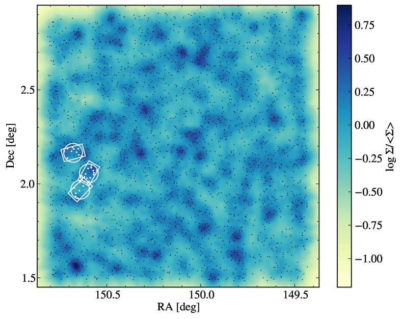
Figure 1.— The density map of the pBzK galaxies in the COSMOS 2 square degree field covered by the K-band image from McCracken et al. (2010). Black and white dots show the location of the $\sim 2800$ pBzKs down to $\mathit{K}=22$ and the spectroscopically observed pBzKs, respectively. White rectangles and circles show the FoVs covered by MOIRCS observations (the mask IDs are B, A, and C from north to south, respectively). Slits were placed in the overlapping regions between a circle and the corresponding rectangle. Background shows the surface density of pBzKs as calculated from 10-th nearest neighbour and normalized by an average surface density of 0.41 arcmin^-2.

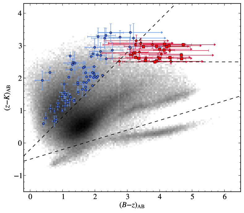
Figure 2.— The BzK 2-color diagram for objects in the COSMOS field. The K-selected objects are shown in gray scale as a background and the pBzKs in our spectroscopic sample are shown in red. Red squares and circles show pBzKs with and without continuum detection, respectively. Blue circles represent star-forming BzK-selected galaxies that were also included in the MOIRCS masks which will be described in a forthcoming paper.

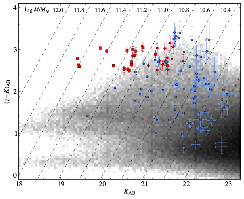
Figure 3.— The $(\mathit{z}-\mathit{K})$–K color–magnitude diagram for objects in the COSMOS field. Symbols are the same as in Figure 2. Dashed lines show constant stellar mass derived by using Equation (6) and (7) of Daddi et al. (2004), i.e., $\log(M_{*}/10^{11}\,M_{\odot}=-0.4(\mathit{K}^{\text{tot}}-21.38)+0.218(\mathit{z}-\mathit{K}-2.29)$, converted to the Chabrier IMF adopted in this paper.

Table 1Photometric properties of observed pBzKs

ID	RA	Dec	$B$	$z$	$K$	$B-z$	$z-K$	$z_{\text{phot}}$	Mask ID	Exp. Time
	(deg)	(deg)	(mag)	(mag)	(mag)	(mag)	(mag)			(min)
Identified
254025	150.6187115	2.0371363	$25.15\pm 0.03$	$22.19\pm 0.02$	$19.41\pm 0.01$	$3.23\pm 0.04$	$2.78\pm 0.02$	1.7407	A	490
217431	150.6646939	1.9497545	$26.11\pm 0.10$	$22.07\pm 0.03$	$19.43\pm 0.01$	$4.32\pm 0.10$	$2.63\pm 0.03$	1.2457	C	450
307881	150.6484873	2.1539903	$26.47\pm 0.13$	$22.06\pm 0.03$	$19.46\pm 0.01$	$4.68\pm 0.13$	$2.60\pm 0.03$	1.4201	B	550
233838	150.6251048	1.9889180	$27.44\pm 0.29$	$22.98\pm 0.05$	$19.95\pm 0.01$	$4.73\pm 0.29$	$3.03\pm 0.05$	1.8428	C	450
277491	150.5833512	2.0890266	$26.31\pm 0.10$	$23.08\pm 0.06$	$20.11\pm 0.01$	$3.50\pm 0.12$	$2.97\pm 0.06$	1.7936	A	490
313880	150.6603061	2.1681129	$25.97\pm 0.07$	$22.88\pm 0.05$	$20.27\pm 0.02$	$3.36\pm 0.09$	$2.61\pm 0.05$	1.3430	B	550
250093	150.6053729	2.0288998	$27.21\pm 0.25$	$23.57\pm 0.09$	$20.59\pm 0.02$	$3.90\pm 0.27$	$2.98\pm 0.09$	1.4234	A	490
263508	150.5677283	2.0594318	$26.77\pm 0.14$	$23.14\pm 0.06$	$20.61\pm 0.02$	$3.90\pm 0.15$	$2.53\pm 0.06$	1.5658	A	490
269286	150.5718552	2.0712204	$26.73\pm 0.14$	$23.14\pm 0.06$	$20.64\pm 0.02$	$3.85\pm 0.15$	$2.50\pm 0.06$	1.6654	A	490
240892	150.6432950	2.0073169	$>27.90$	$23.40\pm 0.08$	$20.69\pm 0.02$	$>4.67$	$2.71\pm 0.08$	1.5474	C	450
205612	150.6542714	1.9233323	$26.32\pm 0.09$	$23.33\pm 0.06$	$20.70\pm 0.02$	$3.26\pm 0.11$	$2.64\pm 0.06$	1.2932	C	450
251833	150.6293675	2.0336620	$26.36\pm 0.12$	$23.07\pm 0.06$	$20.52\pm 0.02$	$3.56\pm 0.13$	$2.55\pm 0.06$	1.1874	A	490
228121	150.5936156	1.9754018	$27.75\pm 0.38$	$23.73\pm 0.10$	$20.73\pm 0.02$	$4.29\pm 0.39$	$3.00\pm 0.10$	1.7198	C	450
321998	150.7093826	2.1863891	$27.50\pm 0.32$	$23.63\pm 0.09$	$20.77\pm 0.02$	$4.13\pm 0.33$	$2.87\pm 0.09$	1.4320	B	550
299038	150.7091894	2.1369001	$>27.90$	$24.02\pm 0.13$	$20.97\pm 0.02$	$>4.15$	$3.05\pm 0.13$	1.7667	B	550
209501	150.6645174	1.9325604	$>27.90$	$24.17\pm 0.14$	$21.56\pm 0.04$	$>4.00$	$2.61\pm 0.15$	1.3413	C	450
253431	150.6408360	2.0378335	$>27.90$	$24.17\pm 0.13$	$21.27\pm 0.03$	$>4.00$	$2.89\pm 0.13$	1.5583	A	490
275414	150.5822420	2.0857211	$>27.90$	$23.76\pm 0.12$	$20.80\pm 0.02$	$>4.22$	$2.96\pm 0.12$	1.4332	A	490
No detection
222961	150.6455001	1.9637953	$>27.90$	$24.76\pm 0.25$	$21.69\pm 0.05$	$>3.41$	$3.07\pm 0.25$	1.4755	C	450
229536	150.6724126	1.9780668	$26.58\pm 0.14$	$24.08\pm 0.16$	$21.56\pm 0.05$	$2.75\pm 0.21$	$2.52\pm 0.17$	1.6066	C	450
243138	150.5947944	2.0130046	$27.46\pm 0.27$	$24.65\pm 0.23$	$21.93\pm 0.06$	$3.08\pm 0.35$	$2.72\pm 0.24$	1.9387	A	280
251051	150.5881329	2.0320317	$27.10\pm 0.20$	$24.21\pm 0.14$	$21.50\pm 0.04$	$3.15\pm 0.24$	$2.72\pm 0.15$	1.4514	A	280
255465	150.6336861	2.0423782	$27.35\pm 0.24$	$24.43\pm 0.16$	$21.66\pm 0.05$	$3.19\pm 0.29$	$2.77\pm 0.17$	1.8805	A	280
258867	150.5698729	2.0491841	$>27.90$	$24.77\pm 0.25$	$21.62\pm 0.05$	$>3.28$	$3.15\pm 0.25$	2.3654	A	280
260120	150.6126504	2.0523735	$>27.90$	$23.82\pm 0.10$	$21.31\pm 0.03$	$>4.35$	$2.51\pm 0.10$	0.9670	A	280
268884	150.5525002	2.0719597	$>27.90$	$24.34\pm 0.17$	$21.31\pm 0.03$	$>3.78$	$3.03\pm 0.17$	1.6244	A	280
273534	150.5994479	2.0819904	$27.50\pm 0.27$	$24.52\pm 0.20$	$21.49\pm 0.04$	$3.25\pm 0.34$	$3.03\pm 0.20$	1.5801	A	280
281751	150.5802008	2.1000786	$27.03\pm 0.18$	$23.72\pm 0.09$	$21.10\pm 0.02$	$3.58\pm 0.20$	$2.62\pm 0.09$	1.1811	A	280
305677	150.6343972	2.1488364	$27.11\pm 0.33$	$23.04\pm 0.09$	$20.52\pm 0.02$	$4.34\pm 0.34$	$2.52\pm 0.09$	1.3697	B	340
315704	150.6874049	2.1729448	$>27.90$	$24.10\pm 0.14$	$21.37\pm 0.04$	$>4.05$	$2.74\pm 0.15$	2.5197	B	550
316338	150.7264016	2.1721785	$>27.90$	$24.08\pm 0.15$	$21.44\pm 0.04$	$>3.95$	$2.64\pm 0.16$	1.1895	B	340
321193	150.6749498	2.1850247	$27.45\pm 0.25$	$24.34\pm 0.16$	$21.54\pm 0.04$	$3.37\pm 0.30$	$2.80\pm 0.16$	1.5988	B	550
322048	150.6514093	2.1861803	$27.18\pm 0.27$	$24.03\pm 0.14$	$20.95\pm 0.03$	$3.42\pm 0.30$	$3.08\pm 0.14$	1.5022	B	340
325564	150.6824812	2.1934154	$>27.90$	$23.57\pm 0.10$	$20.72\pm 0.02$	$>4.31$	$2.85\pm 0.10$	1.3220	B	550

Note. — Upper limits are $3\sigma$.

2.2. Observations

The near-IR multi-object spectroscopic observations have been carried out with Subaru/MOIRCS. The imaging FoV of MOIRCS is $7\times 4$ arcmin² with 2 detectors (channel 1 and 2, respectively) and slits can be placed within the intersection with the 6 arcmin diameter circular region as illustrated in Figure 1. The low resolution zJ500 grism was used with $0.7$ arcsec width slits, which covers about 9000–17500 Å with a resolution $R\simeq 500$. The slit length ranges from 8 to 14 arcsec, adequate to subtract the sky background.

Six masks in total, two masks per FoV, were observed during six separate observing runs as reported in Table 2. We replaced targets with alternative ones when neither continuum emission nor emission lines were seen in the first observing runs, but the majority of the targets are common between the masks targeting the same FoVs (cf. Table 2). Sequences of 600–1200 sec integrations were made in a standard two-position “AB” dithering pattern separated by 2 arcsec. At the beginning and/or end of the nights A0V-type standard stars were observed for flux calibration (i.e., atmospheric absorption and instrument response) with the identical instrumental setup as the targets and with similar airmass as for the COSMOS field observations.

In 2009, observations were affected by cloudy weather and $\sim 1.2$ arcsec seeing whereas in 2010 we took advantage of clear nights and $\sim 0.4$–$1.0$ arcsec seeing conditions. Each FoV was integrated for 7–9 hours (about half of this if targets were replaced between runs). Table 2 summarizes our observations.

Table 2Observation Logs

Mask ID	Date	Exp Time	Number of pBzKs	Number of sBzKs
		(min)
A	13, 14 Mar 2009	280	16 string	16 string
	29, Mar 2010	210	8 (8)	20 (8)
B	6 Feb 2010	340	10 string	17 string
	1 Apr 2010	210	7 (7)	15 (7)
C	7 Feb 2010	330	8 string	15 string
	21 Feb 2010	120	8 (8)	14 (9)

Note. — Column 1: ID of the three MOIRCS pointings (masks); Column 2: observing date; Column 3: exposure time; Column 4: number of pBzKs in the mask; Column 5: number of sBzKs in the mask

2.3. Data Reduction

The data were reduced with the MCSMDP pipeline (Yoshikawa et al., 2010) and with custom scripts. The data are first flat-fielded using dome-flat frames taken with the same configuration of the science frames. Bad pixels were then removed using the bad-pixel map bundled in MCSMDP and cosmic ray hits were removed using the pair of images in the dithering. The counts of the rejected pixels were replaced by linear interpolations from neighboring pixels along the spatial direction. After removing bad pixels and cosmic rays, the sky background was removed by subtracting the “B” frame from the “A” frame. Then the distortion of the detectors was corrected by using the same coefficients used in the MOIRCS imaging data reduction.

Each frame was then rotated to correct the tilt of the spectra on the detector by making the edges of each slit almost parallel to the $x$-direction (dispersion direction) of the detector. We applied a rotation angle of $\sim-0.56$ and $\sim-0.73$ degrees for the channel 1 and 2, respectively.

Individual spectra were cut from the frames and wavelength calibration was made for each extracted 2-dimensional spectrum based on the location of the OH-airglow lines (Rousselot et al., 2000) present in the observed wavelength range. The uncertainty of the wavelength calibration is typically one half the pixel size, i.e., $\sim 2.5$ Å. Then the frame was transformed to align the sky lines along the $y$-direction (spatial direction) and to make wavelength a linear function of pixel coordinates. Because sky background residuals are expected due to the time variation of sky brightness (in particular in the OH-line strength) we performed an additional residual sky-subtraction by subtracting at each wavelength a mean of the spatial pixels outside those occupied by the objects.

The spectra of the A0V-type stars were processed in the same manner as for the targets, and the 2D frames were co-added. Then the 1D spectra of the standard stars were extracted by using the apall task in IRAF. The system response curves including atmospheric, telescope, and instrumental throughputs were obtained by dividing the observed spectra of the standard stars by spectra from the stellar spectral library of Pickles (1998). After the residual sky-subtraction, the 2D spectra of the targeted galaxies were flux-calibrated by dividing them by the system response curve and co-added with appropriate offsets derived either from the location of reference stars or bright compact objects to which slits had been assigned or from the fits header information. In performing these co-additions we applied weights proportional to the exposure time and inversely proportional to the seeing size and the square of the S/N of each individual 2D spectrum.

Finally, for the objects with continuum detection the 1D spectra were extracted from the stacked 2D frames by using the apall task in IRAF. The 1D spectra from the different observing runs were extracted separately, and then the pairs of 1D spectra were stacked together with a weight to maximize the S/N of the final 1D spectra. These 1D spectra were calibrated to absolute flux scale by comparing them with the $J$- and $H$-band fluxes. The uncertainty of the absolute flux calibration is $\lesssim 20$% indicated by the difference of the scaling factor between the $J$ and the $H$ band.

The cutouts from the COSMOS HST/ACS $i$-band image (Koekemoer et al., 2007) and 1D spectra of the 18 pBzKs with continuum detection for which the determination of the spectroscopic redshifts was attempted are shown respectively in the left and middle panels of Figure 4.

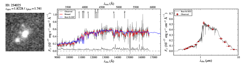
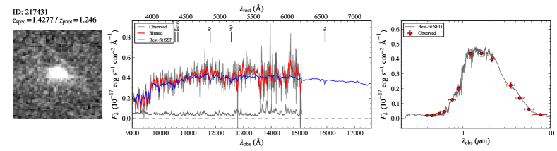
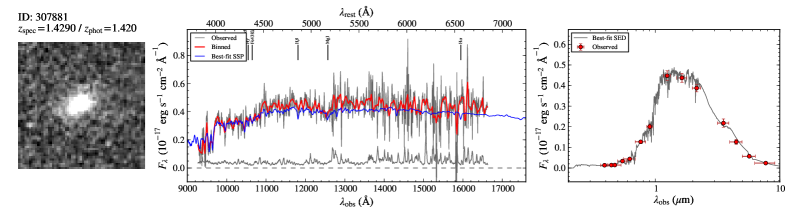
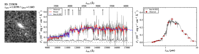
Figure 4.— HST/ACS stamps, MOIRCS spectra, and broad-band SEDs of the continuum detected pBzKs in this study. Left: HST/ACS cutouts made from the publicly available COSMOS HST-ACS Mosaic v2.0 from Koekemoer et al. (2007). The images are 3 arcsec on a side; Middle: MOIRCS spectra. The observed spectrum, its 50 Å median smoothed version, and its best-fit SSP template from Bruzual & Charlot (2003) library are shown respectively in gray, orange, and blue. The gray spectra at the bottom show the $1\sigma$ noise. The positions of major absorption lines are indicated by the vertical lines; Right: Broad-band SEDs. The red circles show the observed fluxes and the gray line shows the best-fit template. The panels from the top to bottom are ordered with increasing total $K$-band magnitude. The IDs and spectroscopic and photometric redshifts are indicated.

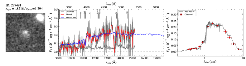
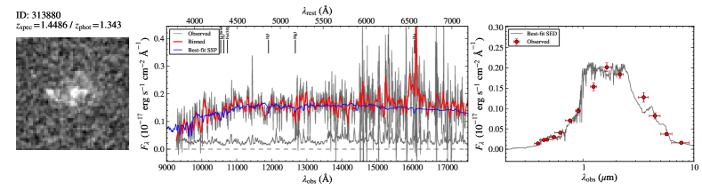
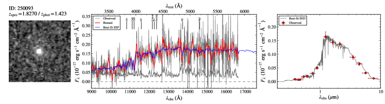
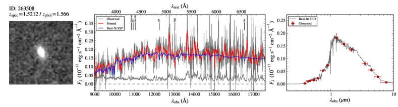
Figure 4.— Continued.

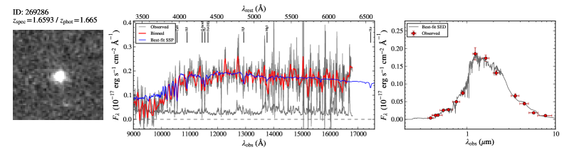
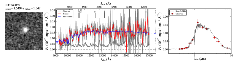
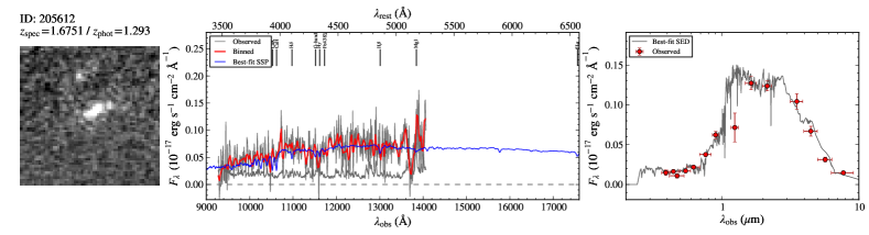
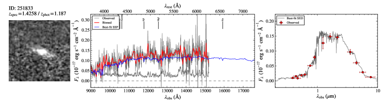
Figure 4.— Continued.

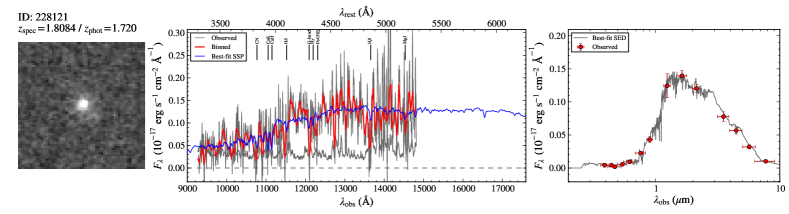
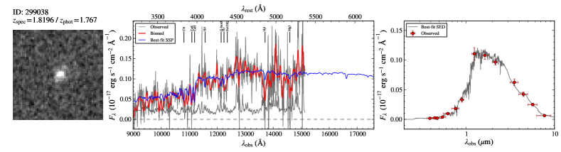
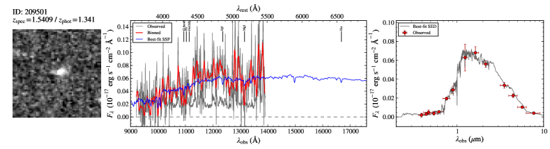
Figure 4.— Continued.

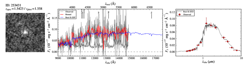
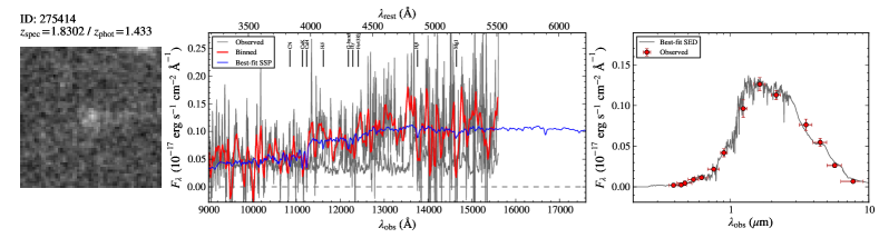
Figure 4.— Continued.

3. Spectroscopic Redshifts

3.1. Redshift Measurement

None of the target objects shows emission lines in the observed spectral range, which supports their identification as PEGs. The measurement of spectroscopic redshifts was therefore attempted from stellar absorption features such as Ca II H+K, the 4000 Å break and Balmer lines. The spectroscopic redshifts were then derived using the Penalized Pixel-Fitting method (pPXF; Cappellari & Emsellem, 2004), using template stellar spectra from the MILES stellar library (Sánchez-Blázquez et al., 2006). We have paid special attention to the error analysis, including systematic effects, in particular those that could be introduced by the spurious sky residuals and the correlated noise. Thus, we have adopted the standard bootstrapping technique of resampling residuals to adjacent groups of spectral pixels, rather than to the individual pixels, to account for the correlated noise, then randomly reshuffling the best-fitting residuals in groups of 50 pixels (300 $\,\text{km}~{}\text{s}^{-1}$), allowing for duplication. These residuals were added to the galaxy spectrum, then fitting the data with pPXF. To account for the sensitivity of the fits to the polynomial degree for each noise realization we adopted a random degree between 0 and 4 for the additive and another random one for the multiplicative polynomials. In the new fits we repeated the entire pPXF procedure, namely redetermining the set of best fitting MILES stellar templates thus finding a new set of $\sigma$-clipped residuals. This procedure was repeated for 300 random realizations and $1\sigma$ errors were derived from the distribution of the output redshifts from the realizations. The results are reported in Table 3 along with their errors.

As a cross-check, redshifts were also derived by cross-correlating with simple stellar population (SSP) templates from Bruzual & Charlot (2003, hereafter BC03) with various ages and metallicities after broadening to $\sigma=300$ $\,\text{km}~{}\text{s}^{-1}$. For all the objects, the resulting redshifts are consistent within $1\sigma$ errors with those derived using stellar templates.

The 18 identified objects are shown with squares in Figure 3. Since the identification is nearly complete (16 out of 19 objects) at the brighter magnitude, $\mathit{K}\lesssim 21$, the primary factor of the spectroscopic identification in this kind of observations appears to be the total K-band magnitude. Moreover, since we have selected all pBzKs brighter than $\mathit{K}<21$ in the observed FoVs, the completeness of the spectroscopic identification is 85% down to this depth.

A redshift confidence class was assigned to each object according to the following criteria: Class 4 is assigned to the objects which clearly show both the 4000 Å break and some absorption lines; Class 3 is assigned to objects with a clear 4000 Å break but without unambiguously recognizable absorption lines; Class 2 refers to redshifts derived from the overall shape of the continuum, i.e., the 4000 Å break is not so prominent; Class 1 is for an insecure redshift. The assigned redshift classes are reported in Table 3. A redshift class $\geq 1$ was assigned to the 18 objects for which the continuum could be detected, whereas for 16 objects no continuum was detected and they are listed separately in Table 1.

Table 3Spectroscopic Properties

ID	$z_{\text{spec}}$	Class	Dn4000	H$\delta_{\text{F}}$
				(Å)
254025	$1.82283\pm 0.00055$	4	$1.40\pm 0.03$	$\phantom{string}2.84\pm 1.30$
217431	$1.42769\pm 0.0015\phantom{0}$	4	$2.03\pm 0.10$	$\phantom{string}6.23\pm 1.10$
307881	$1.42904\pm 0.00089$	4	$2.06\pm 0.08$	$\phantom{string}5.59\pm 1.15$
233838	$1.8199\phantom{0}\pm 0.0016\phantom{0}$	4	$1.53\pm 0.05$	$\phantom{string}2.95\pm 1.30$
277491	$1.8163\phantom{0}\pm 0.0038\phantom{0}$	3	$2.74\pm 0.25$	$\phantom{string}1.30\pm 1.51$
313880	$1.4486\phantom{0}\pm 0.0018\phantom{0}$	2	$1.42\pm 0.09$	$-2.66\pm 1.78$
250093	$1.8270\phantom{0}\pm 0.0010\phantom{0}$	4	$1.49\pm 0.10$	$\phantom{string}6.47\pm 1.22$
263508	$1.52122\pm 0.00094$	2	$1.47\pm 0.09$	$\phantom{string}5.40\pm 1.20$
269286	$1.6593\phantom{0}\pm 0.00058$	3	$1.38\pm 0.06$	$\phantom{string}4.86\pm 1.19$
240892	$1.54939\pm 0.00092$	2	$1.55\pm 0.10$	$\phantom{string}9.03\pm 0.84$
205612	$1.6751\phantom{0}\pm 0.0045\phantom{0}$	2	$1.52\pm 0.09$	$-3.92\pm 1.76$
251833	$1.42578\pm 0.00057$	2	$1.71\pm 0.18$	$-1.80\pm 1.69$
228121	$1.8084\phantom{0}\pm 0.0015\phantom{0}$	2	$1.38\pm 0.12$	$\phantom{string}2.84\pm 1.52$
321998	$1.52263\pm 0.00087$	3	$2.13\pm 0.14$	$-1.25\pm 1.59$
299038	$1.81957\pm 0.00098$	3	$2.06\pm 0.12$	$-4.18\pm 1.77$
209501	$1.5401\phantom{0}\pm 0.0078\phantom{0}$	1	$2.02\pm 0.33$	$\phantom{string}2.07\pm 1.72$
253431	$1.5423\phantom{0}\pm 0.0037\phantom{0}$	1	$1.61\pm 0.21$	$-1.47\pm 1.72$
275414	$1.8302\phantom{0}\pm 0.0147\phantom{0}$	1	$2.01\pm 0.24$	$-1.59\pm 1.63$
Stacked	$\cdots$		$1.54\pm 0.03$	$\phantom{string}4.26\pm 0.40$

3.2. Comparison between Spectroscopic and Photometric Redshifts

Figure 5 shows the comparison between the spectroscopic redshifts derived above and photometric redshifts from Ilbert et al. (2009). This is virtually the first attempt to systematically test the COSMOS 30-band photometric redshift against measured spectroscopic redshift of PEGs at $z>1.4$. A majority of the objects show fairly good agreement between photometric and spectroscopic redshifts, but several outliers also exist. Of course, such outliers can be ascribed to either of the two methods to measure redshifts, and here we briefly try to identify the (main) culprit.

First notice that two outliers have quite secure spectroscopic redshift, having assigned Class 4 (namely, objects 217431 and 250093). For these objects the photometric redshifts are clearly in error. In Figure 6 we show the stacked spectrum (see Section 5) of the 9 objects with low confidence class (1 and 2): several strong features are clearly present in this spectrum, namely Ca II H&K, the G band and Mg$b$, and these features are still recognizable in the stacked spectrum including only the five Class 1 and 2 outliers seen in Figure 5. We conclude that the spectroscopic redshifts are correct also for the majority of these two classes of objects and therefore in the present sample $\sim 30$% of the PEG photometric redshifts are systematically underestimated.

More quantitatively, the average offsets are $\langle z_{\text{spec}}-z_{\text{phot}}\rangle=0.12$ or $\langle(z_{\text{spec}}-z_{\text{phot}})/(1+z_{\text{spec}})\rangle=0.04$, and the standard deviations of $z_{\text{spec}}-z_{\text{phot}}$ and $(z_{\text{spec}}-z_{\text{phot}})/(1+z_{\text{spec}})$ are 0.14 and 0.053, respectively. The normalized median absolute deviation (NMAD; Hoaglin et al., 1983), $\sigma_{\text{NMAD}}=1.48\times\text{median}(\left|z_{\text{spec}}-z_{\text{phot}}\right|/(1+z_{\text{spec}}))$, which is used to estimate the accuracy of the COSMOS photometric redshift by Ilbert et al. (2009), is calculated as 0.050. This is similar to $\sigma_{\text{NMAD}}=0.054$ for the $1.5<z<3$ zCOSMOS-Deep sample with $i^{+}\simeq 24$ (Lilly et al., 2007). However, they found that $\sim 20$% of the 147 zCOSMOS-Deep galaxies at $1.5<z<3$ show catastrophic failure defined as $\left|z_{\text{spec}}-z_{\text{phot}}\right|/(1+z_{\text{spec}})>0.15$, whereas no such large catastrophic failures are found in the pBzK sample presented here. Still, these results indicate that the photometric redshifts from Ilbert et al. (2009) would lead to a systematic underestimate of the volume density of high redshift PEGs, though the present statistics is too limited to precisely quantify the effect.

Notice that all our pBzK selected objects with detected continuum have $z_{\text{spec}}>1.4$, including those with $z_{\text{phot}}<1.4$, indicating that the passive BzK-selection is indeed quite effective to identify bona fide PEGs at $z>1.4$ (see also Section 3.2.1), especially when disregarding mid- and/or far-IR detected objects.

We also note that the clustering of the spectroscopic redshifts around a few redshift spikes (including Class 1 and 2 redshifts, see Section 4) lends support to the correct identification of such redshifts. No such clustering would indeed be expected from random errors in the spectroscopic redshifts, unless spurious breaks were introduced by the flux calibration, which does not appear to be the case.

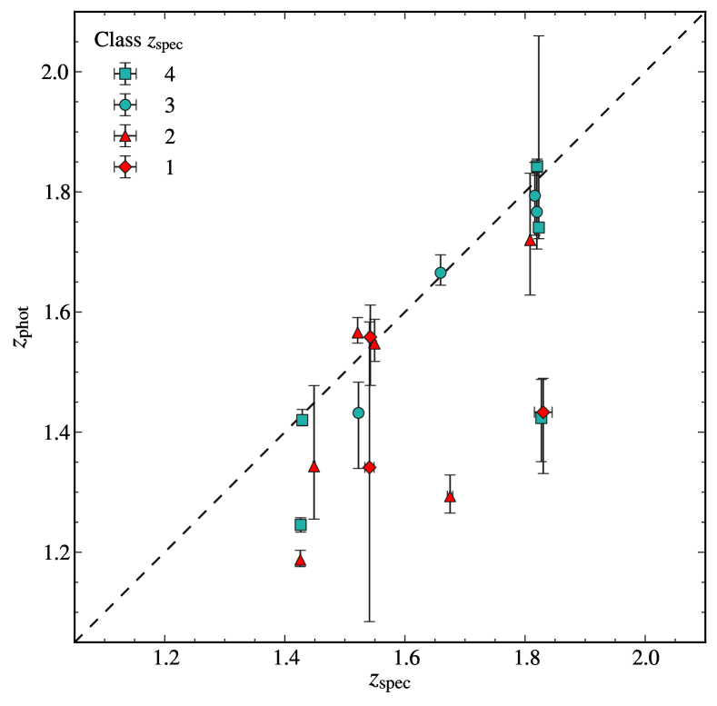
Figure 5.— Comparison between the spectroscopic redshifts of the present study and the photometric redshifts from Ilbert et al. (2009). Different symbols refer to the quality Class of the derived spectroscopic redshifts as defined in the text and shown on the top-left corner of the figure.

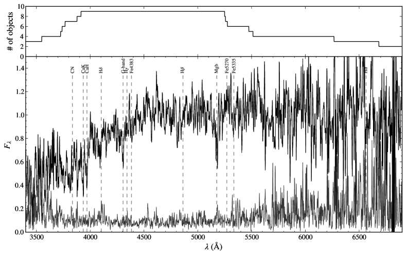
Figure 6.— The composite spectrum of up to 9 pBzKs whose redshifts have Class 1 and 2 (i.e., lower quality). The bottom panel shows the composite spectrum and its $1\sigma$ noise. The locations of major absorption lines are labeled and indicated by dashed-lines. The top panel shows the number of objects used for stacking at each wavelength.

3.2.1 Improving photometric redshifts for high redshift PEGs

To explore the possibility of improving the performance of photometric redshifts, specifically for high-redshift PEGs, we have calculated new photometric redshifts using the 18 spectroscopic redshifts in this work as a training sample. We used EAZY (Brammer et al., 2008) to fit the 14-passband SEDs (UBgVrizJHKs and the 4 IRAC bands, see Section 6.1) of the 18 PEGs, and different sets of templates, namely the EAZY default templates (cf. Brammer et al., 2008, 2011; Whitaker et al., 2011), as well as passive synthetic populations built with Maraston (2005, hereafter M05) and BC03 models, with a suitable range of ages and metallicities.

Following Ilbert et al. (2009), we estimated systematic photometric offsets relative to the default EAZY templates by running EAZY on the 18 PEGs having fixed the redshift to their spectroscopic value. This was done by measuring, for each band, the median offset between the observed flux of the galaxies and the flux of the best-fitting templates, iteratively correcting all passbands until convergence. We note that, besides correcting for possible systematic errors in the photometric zero-points, aperture corrections, and/or in the filter transmission curves, such systematic offsets are specific to the adopted set of templates and reflect their possible limitations. Nonetheless, we show below that adopting the systematic offsets determined with the EAZY templates we obtain consistent photometric redshift estimates also when using the passive BC03 and M05 template sets.

In Figure 7 the resulting $z_{\text{phot}}$ values are compared to the corresponding $z_{\text{spec}}$ for the sample of our 18 PEGs, separately for each of the three template sets. The improvement with respect to the original photometric redshifts is immediately evident. Using EAZY default templates the median of the discrepancy $(z_{\text{spec}}-z_{\text{phot}})/(1+z_{\text{spec}})$ is 0.006, with a scatter $\sigma_{\text{NMAD}}=0.017$. When using M05 and BC03 templates the median of the discrepancy is 0.004 and 0.0009, respectively and $\sigma_{\text{NMAD}}\simeq 0.02$ in both cases.

Of course, we are comparing $z_{\text{spec}}$ and $z_{\text{phot}}$ for the same 18 galaxies used as training sample to determine the systematics offsets. However, within the limits due to the poor statistics, similarly small median discrepancies and scatters are found when using a random half of the sample for training and the other half for checking $z_{\text{spec}}$ vs. $z_{\text{phot}}$. This suggests that the quoted accuracy of the new photometric redshifts is in fact reliable, at least for sources with similar SED, magnitudes and redshift as the PEGs considered here. We note that the Ilbert et al. photometric redshifts were optimized for $z\lesssim 1.3$, using a set of medium bands at optical wavelengths. While they reached better than $\sim 1\%$ accuracy up to $z\sim 1.3$ for bright sources, the performance for fainter sources ($\mathit{i}>24$) and particularly for galaxies at $z\gtrsim 1.3$ is significantly degraded (Ilbert et al., 2009). The larger systematic offset and scatter of the original photometric redshifts (Ilbert et al., 2009) illustrated in Figure 5 may at least partly be ascribed to the lack of PEGs in the zCOSMOS-Deep spectroscopic sample (Lilly et al., 2007) that was used as a training sample, as it was designed to contain only star-forming galaxies.

The 18 PEGs we used for tuning photometric redshifts and determining their accuracy are clearly on the bright tail of the general PEG population at these redshifts. Nonetheless, assuming that photometric redshifts derived as above remain reasonably accurate also for fainter PEGs, we measured the photometric redshifts for all the pBzK MIPS-undetected galaxies in the COSMOS sample (McCracken et al., 2010) and compared their distribution to that obtained with the original photometric redshifts from Ilbert et al. (2009).

Figure 8 shows the $z_{\text{phot}}$ distribution of 90% of the full sample, for which a reliable $z_{\text{phot}}$ could be obtained as judged from the $\chi^{2}$ of the best-fit and from the $z_{\text{phot}}$ probability distribution (dotted black and dark-gray lines, for $z_{\text{phot}}$ estimated with standard EAZY and passive M05 templates, respectively). The solid lines show the distribution of the 50% of the sample with best constrained $z_{\text{phot}}$ (i.e., with the best $\chi^{2}$ values and tightest probability distribution). The dashed light-gray line shows the distribution of photometric redshifts from Ilbert et al. (2009), for 85% of their full sample (after removing 2% of the sources unmatched in the Ilbert et al. catalog or identified as X-ray sources, and a further 13% of sources located in masked areas). Apart from a small shift in the peak of the distribution (from $z\sim 1.5$ to $z\sim 1.7$), it is worth emphasizing that about one third of the sources are located at $z_{\rm phot}<1.4$ according to the Ilbert et al., compared to only a few percent with the new determination trained on the present 18 spectroscopic PEGs. This exercise shows that using spectroscopic high-$z$ PEGs as a training sample can substantially improve the estimation of photometric redshifts for this kind of galaxies, as illustrated by a comparison of Figure 5 and Figure 7.

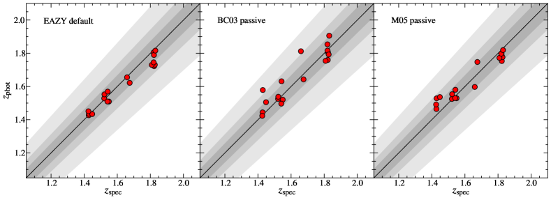
Figure 7.— Comparison between the spectroscopic redshifts from the present study and the corresponding photometric redshifts from different determinations: Left: $z_{\text{phot}}$ from this work using standard EAZY templates; Middle and Right: $z_{\text{phot}}$ from this work using EAZY with passive BC03 and M05 models, respectively (see Section 3.2.1). All EAZY photometric redshifts were obtained using the 18 PEG spectroscopic redshifts in the present study as a training sample. The solid line traces the bisector whereas the filled areas show deviations of $0.025$, $0.05$, and $0.1\times(1+z)$. Readers can refer to Figure 5 for a comparison with the photometric redshift by Ilbert et al. (2009).

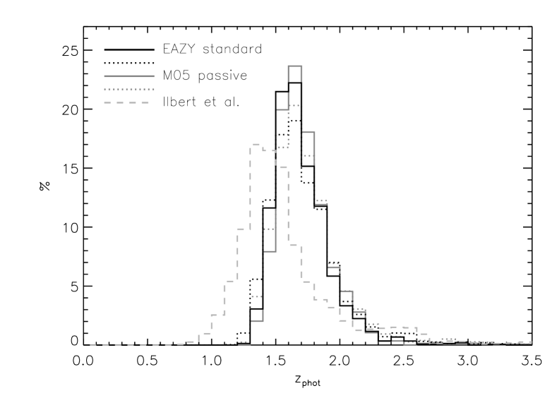
Figure 8.— The distribution of photometric redshifts for pBzK-selected PEGs. The solid/dotted lines show the redshift distribution of 50%/90% of the full PEG sample over the COSMOS field using the photometric redshifts measured in this work using different sets of templates (standard EAZY and passive M05 templates in black and dark gray, respectively). The dashed light-gray line shows the redshift distribution of 85% of the full PEG sample using Ilbert et al. (2009) photometric redshifts. All EAZY photometric redshifts were obtained using the 18 PEG spectroscopic redshifts in this paper as a training sample.

3.3. Note on a MIPS 24 µm source

One of our galaxies pre-selected as a pBzK, i.e., 313880 at $z=1.45$, is detected at Spitzer/MIPS 24 µm with a flux of 130 $\mu\text{Jy}$ which corresponds to a SFR of $\sim 90M_{\odot}\text{yr}^{-1}$, adopting a conversion based on infrared SED templates of Chary & Elbaz (2001) and the Chabrier initial mass function (IMF; Chabrier, 2003). The HST/ACS $i$-band (F814W filter) morphology in Figure 4 suggests that this object has a clumpy disk structure which could be the site of intense star formation (Förster Schreiber et al., 2011; Genzel et al., 2011). Surface profile fitting (see Section 7.1) also shows this object is best fit by an exponential profile. Looking at the spectra in Figure 4, there seems to be an excess of flux at $\sim 1.6$ µm, indicating the presence of H$\alpha$ emission as expected from the relatively high 24 µm flux and infrared-based SFR. However, in the 2D spectra taken during two nights separately as shown in Figure 9, there is no evidence of emission lines and the excess is apparently caused by the residual of the OH sky line subtraction. Other emission lines such as [O III]$\lambda\lambda 4959,5007$ and H$\beta$ are also expected in the J-band where the sky line contamination is less severe than in the H-band, but none of them are detected. The other explanation for non-detection of emission lines is that the object has large amount of dust which attenuates the emission lines below the detection limit, ($3$–$10$)$\times 10^{-17}$ erg s^-1 cm^-2 ($3\sigma$). The SED fit gives $A_{V}=0.55^{+0.34}_{-0.45}$ mag which is one of the highest among the objects in the present sample, but it does not seem enough to attenuate emission lines below detection limits. Given the degeneracy of parameters in SED fitting, the derived $A_{V}$ could possibly be underestimated in this particular case. Here we conclude that this object is probably a star-forming galaxy suffering from heavy dust extinction, and therefore, we excluded it from the stacking analysis (see Section 5).

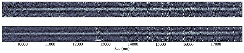
Figure 9.— The two dimensional spectra of the MIPS $24\,\mu\text{m}$ detected source, 313880, taken on February 6, 2010 (Top) and on April 1, 2010 (Bottom). The spectra are 1.9 arcsec wide in the spatial direction.

4. Overdensities of Passively Evolving Galaxies at $z>1.4$

A cursory inspection of Figure 5 is sufficient to realize that spectroscopic redshifts are not randomly distributed, but instead tend to cluster around a few spikes. Indeed, Figure 10 shows the redshift distribution of the 18 spectroscopically identified pBzKs in our 3 masks. There is a clear redshift spike of 7 pBzKs at $z\simeq 1.82$ with $1\sigma$ scatter of 0.006. The projected spatial extent of the overdensity is $\sim 6$ Mpc in diameter and $z=1.82\pm 0.006$ corresponds to $\sim 19$ comoving Mpc along the line of sight. To our knowledge this is the first spectroscopically confirmed overdensity of PEGs at such high redshift.

Another possible redshift-spike at $z\simeq 1.43$ includes 4 pBzKs. Although the significance does not seem high, this $z=1.43$ spike is also noticeable because two of its galaxies are the K-band brightest pBzKs over the whole COSMOS field (Mancini et al., 2010).

A third spike appears to be present at $z\simeq 1.53$, including 5 pBzKs, and the last two galaxies have also close redshifts, around $z\simeq 1.67$. Unfortunately, this area lies outside the zCOSMOS-Deep field, and therefore it is not possible to use its redshifts of star-forming galaxies to check for the presence of spikes at the same redshifts of those reported here. However, a fair number of sBzKs was included in our MOIRCS masks (cf. Table 2) and a comparison of the redshift distributions of pBzKs and sBzKs will be done in a future paper.

Figure 11 shows the location on the sky of the galaxies in these three redshift spikes at $z=1.43$, $1.53$, and $1.82$, together with that of other photo-$z$ selected galaxies with $\Delta z=\pm 0.02$ and $K<23$ from the mean redshift of each spike. There may well be large spikes at these redshifts extending spatially well beyond the area explored by the three MOIRCS FoVs, but our data do not allow us to claim the presence of bound clusters.

The XMM-Newton data (Hasinger et al., 2007; Finoguenov et al., 2007) indicate that there is no extended X-ray emission associated to these redshift spikes down to ($6$–$8$)$\times 10^{-15}$ erg s^-1 cm^-2 ($2\sigma$) in $0.5$–$2$ keV band, which corresponds to the $2\sigma$ limit of $L_{\text{X}}\simeq(1$–$2)\times 10^{44}$ erg s^-1 and $M_{200}\simeq 1.5\times 10^{14}\,M_{\odot}$ at the redshifts of the spikes (A. Finoguenov, private communication).

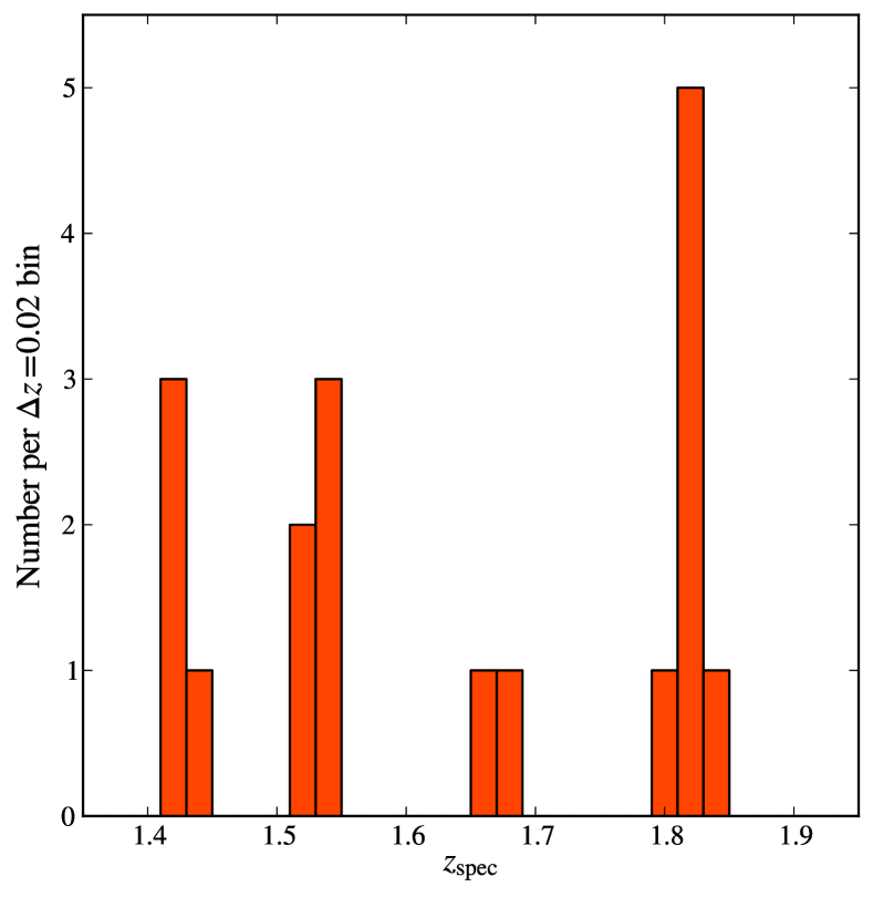
Figure 10.— The redshift distribution of spectroscopically identified pBzKs in the present sample.

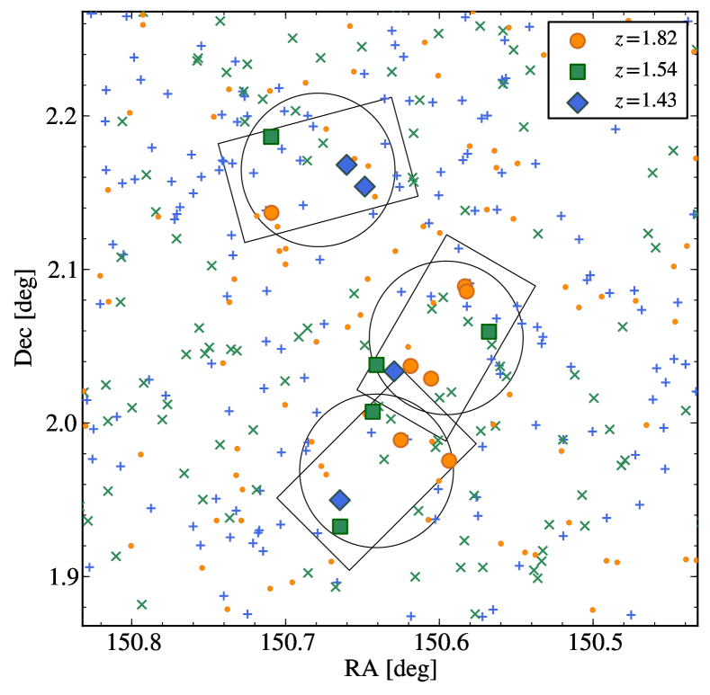
Figure 11.— The spatial distribution of the pBzKs in the three major redshift spikes. The symbols are redshift-coded as indicated in the insert. Small blue pluses, green crosses, and orange circles show objects with $K<23$ and photometric redshift within $\Delta z=\pm 0.02$ from the mean redshifts of the spikes at $z=1.43$, $1.54$, and $1.82$, respectively. Solid boxes and circles represent the position of MOIRCS detectors and masks, respectively.

5. The Composite Spectrum of pBzKs

A composite spectrum has been constructed by stacking 17 out of the 18 spectroscopically identified pBzKs. We excluded the object 313880 because of the MIPS $24\,\mu\text{m}$ detection (see Section 3.3), which could cause a contamination of a star-forming galaxy into a passively evolving population. We did not exclude objects with Class 1 and 2 since the spectroscopic identifications appear to be correct as investigated in Section 3.2 and low-S/N does not affect the result after weighting as described below.

After being de-redshifted to the rest-frame, each individual spectrum was first normalized by the mean flux at rest-frame $4500<\lambda(\text{\AA})<5200$. Then the spectra were linearly interpolated into a 1 Å linearly spaced wavelength grid. The associated noise spectra were normalized by the same factor as that for the object spectrum and interpolated to the rest-frame in quadrature. The spectra were then coadded with weights proportional to the inverse square of the noise spectra at each rest-frame wavelength.

To estimate a realistic error and any biases related to the stacking, we applied the jackknife method to the spectra used for stacking. We made 17 composite spectra in the same way, but removing one object at a time from the stacking. Then the standard deviation of the flux at each wavelength pixel is estimated as

$$\sigma_{\text{Jack}}^{2}=\frac{N-1}{N}\sum_{i=1}^{N}\left(f-f_{(i)}\right)^{2},$$ (1)

where $N$ is a number of objects in the sample (i.e., $N=17$ here), $f$ is a flux of composite spectrum of $N$ spectra, and $f_{(i)}$ is the flux of the composite spectrum made of $(N-1)$ spectra by removing $i$-th spectrum. We use $\sigma_{\text{Jack}}$ as the $1\sigma$ error of the composite spectrum. The composite spectrum was also corrected for a sampling bias derived from the jackknife estimator as

$$f^{\prime}=f-\left(N-1\right)\left(\langle f_{(i)}\rangle-f\right),$$ (2)

where $\langle f_{(i)}\rangle$ is the average of $f_{(i)}$. The typical correction factor due to the bias estimate is $<2$%. We adopt the bias corrected spectrum $f^{\prime}$ as the final composite spectrum, which is inevitably dominated by the objects with highest S/N ratios as well as by observed-frame wavelength less contaminated by the sky residuals.

The composite spectrum obtained in this way (equivalent to a MOIRCS integration time of about 140 hours) is shown in Figure 12. At least 11 spectral lines/features are clearly visible in this spectrum, and identified in Figure 12; specifically, CN, Ca II H&K, H$\delta$, the G band, H$\gamma$, Fe4383, Fe5270, Fe5335, H$\beta$, and Mg$b$. Although the number of stacked objects are small at longer wavelength where contamination from the residual OH-airglow subtraction is severe, there could be an indication of excess flux at the location of H$\alpha$. We have measured the equivalent width (EW) of the potential H$\alpha$ emission line from the stacked spectrum divided by the best-fit model (see Section 6.4) accounting the underlying absorption, and we found $\text{EW}(\text{H$\alpha$})=3.5$–$5$ Å depending on the width of the integration window to derive the EW (1–2.5 times of FWHM of the instrument). In case of $EW=5$ Å, it can be translated into $\text{SFR}=5.6\,M_{\odot}\,\text{yr}^{-1}$ and $1.9\,M_{\odot}\,\text{yr}^{-1}$ for a object at $z=1.69$ with the brightest and median H-band magnitudes, respectively. In addition to H$\alpha$, we have also carried out a similar measurement on the position of [O II]$\lambda 3727$, and found corresponding SFR of $4\,M_{\odot}\,\text{yr}^{-1}$ and $1.6\,M_{\odot}\,\text{yr}^{-1}$ for the brightest and median cases with an error of about 20-40%. Looking at the individual spectra extending to H$\alpha$, 307881 is the brightest and could mainly contribute to this feature in the composite spectrum. However, the feature around H$\alpha$ in the spectra of 307881 appears to be rather broad, mostly contaminated by adjacent OH residuals. Indeed, when we remove this object from the stacking, the feature disappeared, while the estimated SFR at the position of [O II] still remains the same. Therefore, the residual star formation, if any, could be at most $\sim 5\,M_{\odot}\,\text{yr}^{-1}$ and most likely $<1$–$2\,M_{\odot}\,\text{yr}^{-1}$, which is $>100$–$200$ times smaller than those of galaxies with $M_{\star}=10^{11}\,M_{\odot}$ on the star formation main sequence at $z=2$ (e.g., Daddi et al., 2007; Pannella et al., 2009; Rodighiero et al., 2011). The composite spectrum is analyzed is Section 6.4.

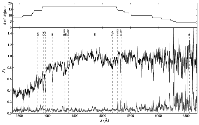
Figure 12.— The same as Figure 6, but now co-adding the spectra of all 17 MIPS-undetected pBzKs in the present sample.

6. Stellar Population Properties of the Program Galaxies

6.1. Broad-band SED Fitting

Having fixed the redshifts to their spectroscopic values, we have derived the physical properties of the galaxies from their broad-band SEDs. Besides the Subaru/Suprime-Cam B and z’ band and CFHT/WIRCam $K$-band photometry to apply the BzK selection technique, we used the multi-band photometry including the CFHT/MegaCam u band, the Subaru/Suprime-Cam g’, V, r’, and i’ bands, and the CFHT/WIRCam J and H bands as well as the four Spitzer/IRAC bands. All magnitudes from u to $K$ are converted to total magnitudes by applying aperture corrections both for point sources and for extended objects (McCracken et al., 2010; Mancini et al., 2011). The IRAC band magnitudes are corrected to the total magnitude following Ilbert et al. (2009).

The SED fitting was carried out by using FAST (Fitting and Assessment of Synthetic Templates; Kriek et al., 2009). FAST includes internal dust reddening and provides various physical quantities of the galaxies such as stellar mass, age, and metallicity. For the templates, we used the composite stellar population models generated from the SSPs of Charlot & Bruzual (2007, in preparation; hereafter CB07) with the Chabrier IMF. It has been argued that the IMF may not be universal among local early-type galaxies, but could depend on the galaxy stellar mass (Cappellari et al., 2012). If so, the masses derived here would be underestimated by up to a factor 2–3 for the most massive objects. We assume a universal IMF in this paper, as it was done in all other similar studies to which we compare our results.

The adopted star formation histories (SFHs) assume an exponentially declining SFR with various $e$-folding times ($\tau$) ranging from $\log(\tau/\text{yr})=7.0$ to $10$ with an interval of $\Delta\log\tau=0.1$ and ages ranging between $\log\text{(age/yr)}=7.0$ to $10$ with an interval of $\Delta\log\text{age}=0.05$. The metallicity $Z$ is fixed for each model (no attempt is made at mimicking chemical evolution) and is chosen from the set $Z=0.004$, $0.008$, $0.02$, and $0.05$. Dust extinction was also applied following the recipe by Calzetti et al. (2000) with $A_{V}=0$–$3$ mag with an intervals of $0.05$ mag. Ages are required to be less than the age of the Universe at the observed redshift. The time-like free parameters in the fit are therefore the age and $\tau$.

Then the best values and 68% confidence intervals of the stellar mass, timescale of the star-formation ($\tau$), age from the onset of star formation, reddening, and metallicity for each galaxy are derived based on the likelihood distribution of each template. The SFR-weighted ages are also computed by using the best-fit $\tau$ and age. Derived physical parameters are listed in Table 4 and the observed galaxy SEDs and the best-fit templates are shown in the right panels of Figure 4.

All but a few of the pBzKs have SEDs consistent with $A_{V}<0.4$ or $E(B-V)<0.1$, i.e., as expected the derived dust extinction is very small for most of the objects. When considering that reddening and age are partly degenerate one can conclude that none of our objects suffers major dust obscuration, as expected for passive galaxies. Stellar population age of the pBzKs are typically $\gtrsim 2$ Gyr. All best-fit SEDs have a short e-folding time $\tau\lesssim 500\,\text{Myr}$ which is typically much shorter than the derived age, i.e., the present star formation is already well suppressed. Stellar masses range from $\sim 4\times 10^{10}\,M_{\odot}$ to $\sim 4\times 10^{11}\,M_{\odot}$, whereas best fit metallicities are near-solar or slightly sub-solar with large uncertainties that cover well above the solar metallicity.

It has been recently argued that an increasing SFR is more appropriate than a declining one in the case of high-redshift star-forming galaxies (e.g., Renzini, 2009; Maraston et al., 2010; Papovich et al., 2011). In particular, an exponentially increasing SFR has been suggested, with $\text{SFR}\propto\tau^{-1}\exp(+t/\tau)$ where $\tau\simeq 500$ Myr. In the case of pBzKs such SFR needs to be truncated at some point, in order mimic the quenching of their star formation. Most galaxies in the present sample show a strong 4000 Å break and some of them strong Balmer absorption lines (see Section 6.3), indicating that the age of the dominant stellar populations must be $\gtrsim 1$ Gyr, hence star formation has to be quenched $\gtrsim 1$ Gyr before the observed epoch. As shown in Table 4, assuming instead a declining SFR the best fit star formation timescale turns out to be typically about 10 times shorter than the age of the galaxies which is well in excess of 1 Gyr. Therefore, for these quenched galaxies both exponentially declining and increasing star formation scenarios would result in almost identical stellar population properties being selected by the best fit procedure.

Table 4Physical Parameters from Broad-band SED Fitting

ID	$\log M_{\star}$	$\log\tau$	$\log t_{0}$	$\log t_{\text{sf}}$	$A_{V}$	$Z$
	($M_{\odot}$)	(yr)	(yr)	(yr)	(mag)
254025	$11.39_{-0.03}^{+0.15}$	$8.20_{-0.15}^{+0.20}$	$9.10_{-0.11}^{+0.20}$	$9.04$	$0.20_{-0.20}^{+0.09}$	$0.008_{-0.004}^{+0.018}$
217431	$11.57_{-0.15}^{+0.03}$	$8.70_{-0.25}^{+0.01}$	$9.60_{-0.23}^{+0.00}$	$9.54$	$0.25_{-0.10}^{+0.25}$	$0.008_{-0.004}^{+0.011}$
307881	$11.50_{-0.11}^{+0.03}$	$8.60_{-0.24}^{+0.04}$	$9.55_{-0.17}^{+0.04}$	$9.50$	$0.20_{-0.11}^{+0.15}$	$0.008_{-0.003}^{+0.008}$
233838	$11.39_{-0.25}^{+0.16}$	$8.30_{-1.30}^{+0.22}$	$9.30_{-0.31}^{+0.20}$	$9.25$	$0.20_{-0.15}^{+0.34}$	$0.008_{-0.004}^{+0.013}$
277491	$11.31_{-0.12}^{+0.11}$	$8.20_{-0.11}^{+0.35}$	$9.05_{-0.06}^{+0.31}$	$8.98$	$0.60_{-0.59}^{+0.05}$	$0.020_{-0.013}^{+0.030}$
313880	$10.85_{-0.27}^{+0.19}$	$8.10_{-1.10}^{+0.48}$	$9.05_{-0.13}^{+0.34}$	$9.00$	$0.55_{-0.45}^{+0.34}$	$0.008_{-0.004}^{+0.016}$
250093	$11.00_{-0.08}^{+0.13}$	$8.10_{-0.14}^{+0.35}$	$9.05_{-0.12}^{+0.26}$	$9.00$	$0.20_{-0.12}^{+0.41}$	$0.020_{-0.014}^{+0.013}$
263508	$10.86_{-0.21}^{+0.10}$	$7.90_{-0.90}^{+0.59}$	$9.00_{-0.11}^{+0.38}$	$8.96$	$0.35_{-0.35}^{+0.22}$	$0.020_{-0.015}^{+0.015}$
269286	$11.01_{-0.28}^{+0.02}$	$8.40_{-1.40}^{+0.12}$	$9.40_{-0.43}^{+0.06}$	$9.35$	$0.00_{-0.00}^{+0.16}$	$0.004_{-0.000}^{+0.017}$
240892	$11.04_{-0.13}^{+0.19}$	$8.40_{-1.40}^{+0.22}$	$9.40_{-0.17}^{+0.20}$	$9.35$	$0.00_{-0.00}^{+0.24}$	$0.020_{-0.013}^{+0.005}$
205612	$10.90_{-0.06}^{+0.13}$	$8.30_{-0.11}^{+0.15}$	$9.15_{-0.07}^{+0.11}$	$9.08$	$0.20_{-0.20}^{+0.10}$	$0.020_{-0.004}^{+0.014}$
251833	$10.74_{-0.05}^{+0.27}$	$8.20_{-0.35}^{+0.43}$	$9.10_{-0.22}^{+0.35}$	$9.04$	$0.30_{-0.20}^{+0.57}$	$0.020_{-0.014}^{+0.019}$
228121	$11.14_{-0.03}^{+0.14}$	$8.40_{-0.20}^{+0.21}$	$9.35_{-0.10}^{+0.20}$	$9.30$	$0.00_{-0.00}^{+0.30}$	$0.020_{-0.014}^{+0.010}$
321998	$11.03_{-0.09}^{+0.12}$	$8.50_{-0.14}^{+0.21}$	$9.45_{-0.12}^{+0.15}$	$9.40$	$0.05_{-0.05}^{+0.28}$	$0.020_{-0.012}^{+0.016}$
299038	$11.05_{-0.15}^{+0.08}$	$8.40_{-1.40}^{+0.12}$	$9.40_{-0.42}^{+0.10}$	$9.35$	$0.10_{-0.10}^{+0.34}$	$0.008_{-0.002}^{+0.017}$
209501	$10.62_{-0.13}^{+0.19}$	$8.40_{-1.40}^{+0.30}$	$9.35_{-0.35}^{+0.25}$	$9.30$	$0.00_{-0.00}^{+0.41}$	$0.020_{-0.013}^{+0.012}$
253431	$10.73_{-0.30}^{+0.23}$	$8.40_{-1.40}^{+0.32}$	$9.35_{-0.43}^{+0.25}$	$9.30$	$0.35_{-0.35}^{+0.36}$	$0.008_{-0.004}^{+0.018}$
275414	$11.05_{-0.24}^{+0.16}$	$8.30_{-1.30}^{+0.23}$	$9.30_{-0.35}^{+0.18}$	$9.25$	$0.20_{-0.20}^{+0.37}$	$0.008_{-0.004}^{+0.018}$

6.2. Rest-frame UVJ colors

Passively evolving galaxies are known to lie in a distinct region on rest-frame $(\mathit{U}-\mathit{V})$ vs. $(\mathit{V}-\mathit{J})$ two-color diagram (e.g., Wuyts et al., 2007; Whitaker et al., 2011). This can be used to check the passive nature of pBzKs in the present sample. Figure 13 shows the UVJ diagram where we have adopted the identical filter combination as that used in Whitaker et al. (2011), namely the Johnson UBV system (Maíz Apellániz, 2006) and the 2MASS J band. The rest-frame UVJ colors were computed by convolving the best-fit templates with the filter response curves without applying atmospheric and instrumental throughputs. The selection box for passive galaxies is defined as $(\mathit{U}-\mathit{V})>0.8\times(\mathit{V}-\mathit{J})+0.7$, $(\mathit{U}-\mathit{V})>1.3$, and $(\mathit{V}-\mathit{J})<1.5$, and young and old galaxies are further separated at $(\mathit{V}-\mathit{J})=0.9$ following Whitaker et al. (2012).

As shown in Figure 13, most of objects have rest-frame UVJ colors consistent with passive evolution. The colors of some outliers are still within $\sim 0.2$ mag from the selection box, and have an offset consistent with possible systematics in the SED fitting and photometric errors. In fact, galaxies with stellar ages of $\gtrsim 1$ Gyr can still be found around $(\mathit{U}-\mathit{V})\simeq 1.7$ and $(\mathit{V}-\mathit{J})\simeq 1.5$ (Whitaker et al., 2012). The MIPS 24 µmsource, 313880, is well within the selection box for passive galaxies, which suggests that the object may be a contaminant to the UVJ selection, or is affected by systematics in the SED fitting. From this UVJ color test we conclude that in all 18 objects star formation has been already quenched, or is very low.

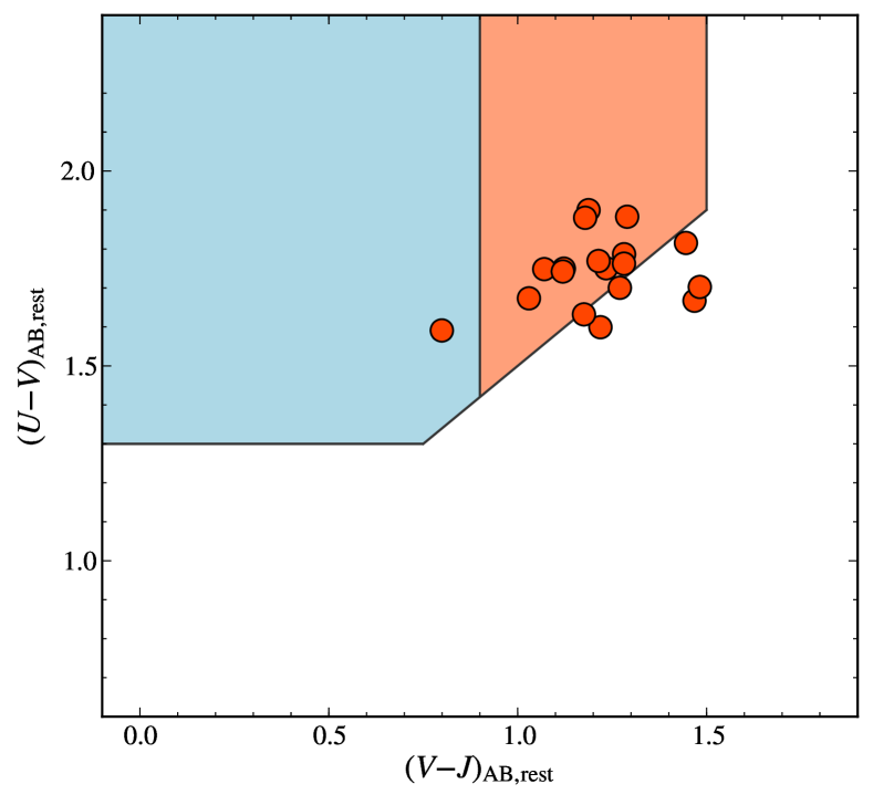
Figure 13.— The rest-frame $(\mathit{U}-\mathit{V})$–$(\mathit{V}-\mathit{J})$ diagram for the 18 pBzKs in the sample (circles). The colored areas represent the selection box for young (blue) and old (red) passively evolving galaxies, respectively, following the definition by Whitaker et al. (2012).

6.3. Rest-frame Optical Absorption Line Indices and the Dn4000 Index

To further characterize the stellar population content of the pBzKs in this sample some of the Lick indices and the strength of the 4000 Å break were measured on our rest-frame optical spectra. To this end we used the Lick_EW program as a part of the EZ_Ages IDL code package (Graves & Schiavon, 2008; Schiavon, 2007), following the definition of the Lick indices by Worthey et al. (1994) and Worthey & Ottaviani (1997). For this purpose one needs to specify a stellar velocity dispersion and the instrument dispersion: we adopted 27 Å in the observed frame for the FWHM of the instrument configuration, and a stellar velocity dispersion of $\sigma_{*}=270$ $\,\text{km}~{}\text{s}^{-1}$ for 254025 (see Section 7.4). For all other objects we used the stellar mass–stellar velocity dispersion relation of local galaxies at $0.05<z<0.07$, determined by using stellar velocity dispersions from the NYU Value-Added Galaxy Catalog (Blanton et al., 2005) and stellar masses from the MPA-JHU catalog (Kauffmann et al., 2003; Salim et al., 2007). The stellar masses of SDSS galaxies are converted to a Chabrier IMF from a Kroupa IMF Kroupa (2001), albeit the correction factor for the velocity dispersions is small ($\sim 10$% and $3.5$% increases for the stellar mass and stellar velocity dispersion, respectively). It is quite possible that high redshift PEGs are more compact than local ones (cf. Section 7.1 below), hence may have higher velocity dispersion compared to the local $M_{*}-\sigma$ relation. However, we use here the local relation because with the exception of the value reported by van Dokkum et al. (2009), all other objects at $z>1.4$ with measured $\sigma$ still follow such relation (Cappellari et al., 2009; Cenarro & Trujillo, 2009; Onodera et al., 2010; van de Sande et al., 2011).

Given the low-S/N of our spectra (typically $\text{S/N}<5$ in the 60 $\,\text{km}~{}\text{s}^{-1}$ interval) and the pixel to pixel fluctuations in S/N due to sky emission lines, we modified the Lick_EW code to use median flux values to compute the pseudo-continua for the indices. Moreover, absorption lines are not clearly visible in most of the spectra, and therefore we restricted our analysis only to objects in which lines are clearly detected and allow a fairly accurate measurement of the relative index. Measurements have been carried out for all objects. In particular, here we focus on the H$\delta_{\text{F}}$ index, which is less affected by OH lines and by emission line filling, if any. Ideally, $\text{H}\beta$ would be a more useful index because it is relatively isolated from other metal absorption lines, hence independent of metallicity of the stellar population. However, for many of our objects $\text{H}\beta$ is strongly contaminated by sky emission lines.

Besides the H$\delta_{\text{F}}$ index, we measured the strength of 4000 Å break as quantified by the Dn4000 index, for which we follow the definition of Balogh et al. (1999) which uses relatively narrow wavelength windows ($\Delta\lambda=100$ Å) for red and blue continua. The Dn4000 index is more robustly derived because the wavelength intervals are wider than those used for absorption line indices. Errors on Dn4000 were estimated through Monte Carlo simulations by artificially adding random noise assuming the normal distribution based on the error spectra at each wavelength pixel. Then 68-percentile intervals are derived from 10,000 realizations per object.

Figure 14 shows the zoom-in of the spectra around H$\delta$ for the objects with high-S/N ($\text{S/N}>5$) for which the absorption line is relatively well detected. On the other hand, Figure 15 shows the spectra around the 4000 Å break for all objects with spectroscopic redshift. For almost all the objects, Dn4000 appears to be measured reasonably well, while for the objects not shown in Figure 14 the region around H$\delta$ is dominated by the noise.

Figure 16 shows the Dn4000 and H$\delta_{\text{F}}$ as a function of the stellar mass, along with the corresponding relation for local galaxies at $z\simeq 0.06$ extracted from the MPA-JHU SDSS database (Kauffmann et al., 2003), corrected for emission line filling. Local galaxies fall in two sequences, one for passive galaxies with higher Dn4000 and lower H$\delta_{\text{F}}$ at a given stellar mass, and another for star-forming galaxies with lower Dn4000 and higher H$\delta_{\text{F}}$.

The objects with S/N $>5$ are also the most massive pBzKs in the sample. As illustrated in Figure 17 which shows H$\delta_{\text{F}}$ as a function of Dn4000, two among them (217431 and 307881) show simultaneously high Dn4000 ($\sim 2$, comparable to those of the local early-type galaxies) and high H$\delta_{\text{F}}$ ($\sim 5$ Å), much stronger than typical of local PEGs of similar stellar mass. A combination of high Dn4000 ($>1.5$) and high H$\delta_{\text{F}}$ ($>3$ Å) appears to be typical of local and moderate redshift post-starburst galaxies (e.g., Vergani et al., 2010), although in this particular case the combination (Dn4000, H$\delta_{\text{F}}$) $\simeq(2,5)$ appears to be rather extreme (cf. e.g., Le Borgne et al., 2006). This can be also seen in Figure 17 in which the location of these two objects cannot be explained by any of the overplotted star formation histories, namely instantaneous burst, exponentially declining SFR, constant and exponentially increasing SFR with truncation. We cannot exclude that Dn4000 may have been somewhat overestimated, given the relatively narrow wavelength range available shortwards of the break (see the corresponding spectra in Figure 4), although the sensitivity curves used for the flux calibration are still smooth and do not suffer from a sharp drop at the edge. By taking these indices at face value, we suggest that these two galaxies may have been quenched a relatively long time ago compared to the star formation timescale, which makes Dn4000 larger, and experienced a recent episode of star formation which has enhanced the H$\delta$ absorption, although it appears to be difficult to enhance H$\delta_{\text{F}}$ without changing significantly Dn4000.

The spectra of the two other objects with high S/N and the composite spectrum show a Dn4000 and H$\delta_{\text{F}}$ combination more akin that of local star-forming galaxies. However, there are virtually no local star forming galaxies with comparable stellar mass and Dn4000 as at this stellar mass almost all local galaxies are already passive since many Gyr. This is also the case for H$\delta_{\text{F}}$ as there is almost no local counterpart with similar stellar mass and H$\delta_{\text{F}}$. The location of these two galaxies in Figure 17, i.e., $\text{Dn4000}\simeq 1.5$ and $\text{H$\delta_{\text{F}}$}\simeq 3$ Å, are typical of the early stages of a post-starburst, i.e., of a very recently quenched galaxy (Balogh et al., 1999).

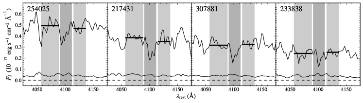
Figure 14.— Zoom-in of the spectra around H$\delta$ for the four objects with the highest S/N ratio. The solid line in each panel shows the object spectrum and the corresponding $1\sigma$ noise. The left and right gray-shaded regions indicate respectively the blue and red continuum windows used used in the definition of the $\text{H}\delta_{F}$ index, whereas the central ones show the window including the H$\delta$ absorption line. The horizontal thick lines indicate the level of blue and red continua for each object. The noise spectrum is shown at the bottom of each panel.

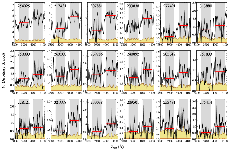
Figure 15.— Zoom-in of the spectra around the 4000Å break. The solid line in each panel shows the spectrum and their $1\sigma$ noise is shown by the light-yellow shaded regions. The gray shaded regions indicate the blue and red continuum windows used to measure the Dn4000 index, and the horizontal thick lines indicate the adopted continuum level on each side of the break. The brown shaded region at the bottom of each panel represents the $1\sigma$ noise divided by $\sqrt{100}$ (the size of each continuum window), which shows the level of the effective noise associated to the flux in these continuum windows.

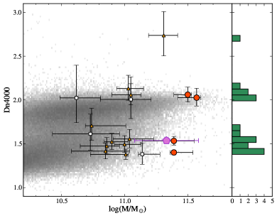
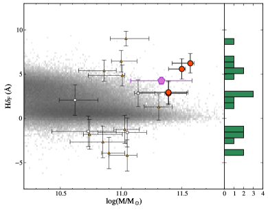
Figure 16.— Left: the Dn4000 index as a function of stellar mass for the 18 pBzKs with spectroscopic redshifts. Right: the H$\delta_{F}$ index as a function of stellar mass. The number of objects in each bin of Dn4000 and H$\delta_{\text{F}}$ are shown as histograms on the right panel of each plot. Individual objects are shown with red circles, yellow triangles, and white squares corresponding to $\text{S/N}>5$, $3<\text{S/N}<5$, and $\text{S/N}<3$ in 60 $\,\text{km}~{}\text{s}^{-1}$ bins, respectively. The pink pentagon refers to the composite spectrum where the stellar mass is a S/N-weighted average among those used for the stacking. The underlying gray shaded area shows the distribution of the local SDSS galaxies including both passive and star-forming objects, after correction for emission line filling in the case of emission line galaxies.

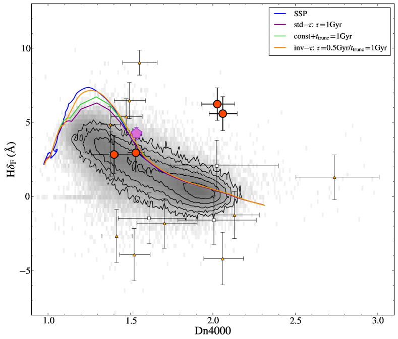
Figure 17.— The $\text{H}\delta_{F}$ vs. Dn4000 plot; symbols correspond to those in Figure 16. The contours show the distribution of the local SDSS passive galaxies whereas the gray shaded area refers to both passive and star-forming local SDSS galaxies. The solid lines show the evolution of stellar populations with various star formation histories (SFH): an instantaneous burst (i.e., a SSP, blue), exponentially declining SFHs with $e$-folding time of 1 Gyr (purple), constant star formation rate over 1 Gyr followed by instantaneous quenching to $\text{SFR}=0$ (green), and exponentially increasing star formation rate with $\tau=0.5$ Gyrs with a truncation at 1 Gyr (orange), as also indicated in the insert. The CB07 evolutionary synthesis models have been used.

6.4. Stellar Populations and Star Formation History from the Composite Spectrum

The high S/N of the composite spectrum allows us to study the “average” stellar population content of our PEGs at $z>1.4$ by using both the detailed shape of the continuum and the absorption lines. For this purpose, we used STARLIGHT (Cid Fernandes et al., 2005, 2009). STARLIGHT is a program to fit an observed spectrum with a combination of template spectra which usually consist of population synthesis models. These template spectra are selected from the CB07 SSP library spanning 29 ages logarithmically spaced between 10 Myrs and 5 Gyrs (the age of the Universe at $z=1.4$ is $\sim 4.5$ Gyrs) and 4 metallicities from $Z=0.004$ to $Z=0.05$. No intrinsic reddening was assumed as there are no emission lines in the composite spectrum indicative of a star formation activity. We leave the total velocity dispersion and velocity offset as free parameters.

The results of the fitting by STARLIGHT are shown in Figure 18. The composite spectrum is well reproduced by the model with the rms of the residual being $\lesssim 8\%{}$ of the observed flux and with a reduced-$\chi^{2}=1.02$. The composition of stellar populations giving the best fitting spectra is shown in the leftmost panels of Figure 19. The light at 4020 Å is dominated by $400$–$800$ Myr stellar populations with $Z=2.5Z_{\odot}$, whereas the mass is dominated by $\sim 3$ Gyr old stellar populations, again with $Z=2.5Z_{\odot}$. The luminosity and mass weighted ages are $\langle\log t/\text{yr}\rangle_{L}=9.01$ and $\langle\log t/\text{yr}\rangle_{M}=9.59$, respectively.

To check the dependence on the choice of template spectra, the composite spectrum was fitted by restricting the metallicity within the range $Z=0.008$–$0.02$ and/or dropping the templates with age less than $100$ Myrs. The quality of the fit is essentially indistinguishable from the previous one, with a reduced-$\chi^{2}=1.02$–$1.14$ and the resulting SFHs are also shown in Figure 19. There is no indication for the presence of young stellar population with age of $\lesssim 400$ Myr in all fitting results, i.e., there is no detectable B-type star contribution, consistent with the strong Balmer absorption lines (mainly produced by A-type stars) seen in the composite spectrum. The lack of B-type stars is also consistent with no emission line being detected in the residual spectrum in Figure 18. When the metallicity range is limited to sub-solar (two rightmost panels, using only templates with $Z=0.004$ and $0.008$), the composite spectrum is reproduced by a $\sim 1$ Gyr old stellar population formed in an almost instantaneous burst. On the other hand, if solar or super-solar metallicities are allowed in the fitting, the mass results to be dominated by $\gtrsim 3$ Gyr old stellar populations with a small amount of younger, $\sim 400$–$800$ Myr old stellar populations, very similar to SFR-weighted ages derived from SED fitting.

An independent check has been carried out by doing the spectral fitting using the pPXF routine (Cappellari & Emsellem, 2004). The fit used as templates a set of 210 MILES SSP (Vazdekis et al., 2010; Falcón-Barroso et al., 2011) with a Kroupa IMF Kroupa (2001) arranged in a regular grid of 35 different ages, logarithmically spaced between 0.1 and 5 Gyr, and 6 metallicities, namely $\text{[M/H]}=-1.71$, $-1.31$, $-0.71$, $-0.40$, $0.00$, and $0.20$. To reduce the noise in the recovery of the SFH and metallicity distribution we employed linear regularization of the weights during the fitting (Press et al., 1992), as implemented in the current version of pPXF. The regularization level was adjusted to increase the $\chi^{2}$ from the best un-regularized fit by $\Delta\chi^{2}=\sqrt{2\times N_{\rm pix}}$, with $N_{\rm pix}$ the number of spectral pixels. In this way the solution represents the smoothest one that is still consistent with the observed spectrum. The obtained result is shown in Figure 20 as a mass fraction within each age and metallicity interval. Since the best-fit spectrum is indistinguishable from that from STARLIGHT, we do not show it here. The inferred distribution is dominated by a $\sim 2.5$ Gyr stellar populations with solar to super-solar metallicities, with at most a small ($<1$%) contribution from young (100-200 Myr) populations. The mass-weighted age is $\langle\log t/{\rm yr}\rangle_{M}=9.40$, which is very close to that found using STARLIGHT.

These results show once more the effects of the well known age–metallicity degeneracy, in particular, from the fit with pPXF which produces nearly constant contours along a line with decreasing age and increasing metallicity. Combining the two completely independent experiments, derived by using different codes and spectral libraries, any significant contribution from young populations can be excluded and we can conclude that the composite spectrum is well fitted by old ($\gtrsim 1$ Gyr), metal-rich stellar populations. The very small contributions by $\lesssim 400$ Myr old populations found by STARLIGHT and by $\sim 200$ Myr old populations found by pPXF are not significant, and should rather be interpreted as upper limits.

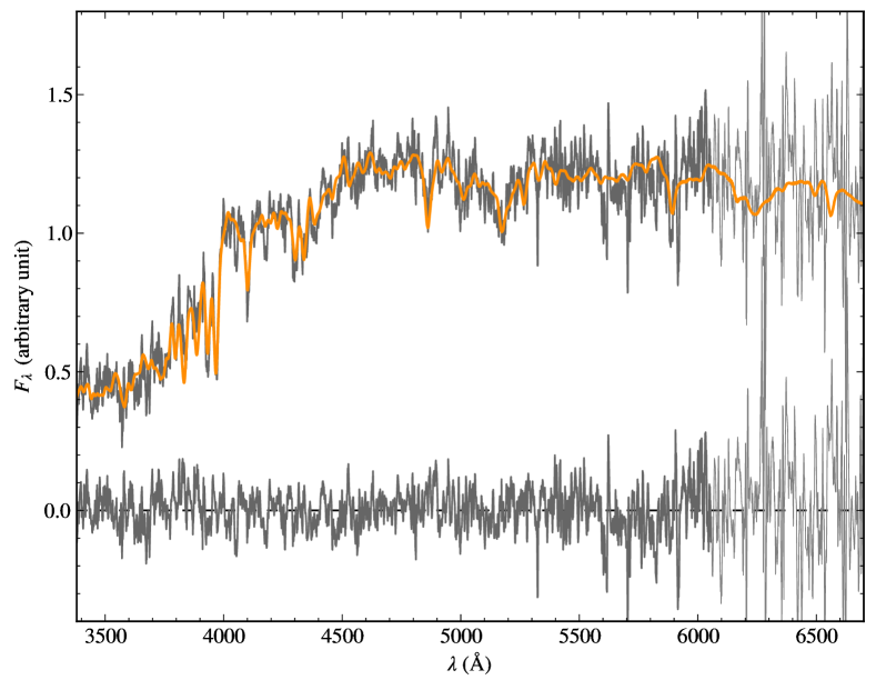
Figure 18.— The STARLIGHT fit to the composite spectrum. The gray line is the composite spectrum being thicker in the wavelength range used for the fit. The orange line shows the STARLIGHT best fit model having allowed age and metallicity to span the $0.01<\text{Age(Gyr)}<5$ and $0.004<Z<0.05$ ranges. The gray line around zero gives the difference between the model and composite spectrum.

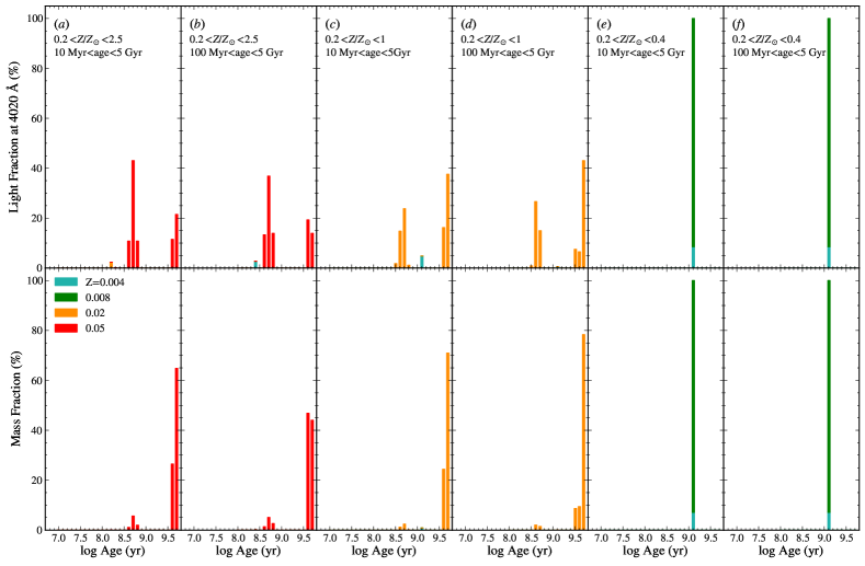
Figure 19.— The age and metallicity distributions of the stellar populations resulting from the STARLIGHT best fit to the composite spectrum. The distributions refer to the fractional contributions to the light at 4020 Å (top) and mass (bottom). On each top panel the age and metallicity ranges allowed during the fit are indicated, whereas metallicities are color-coded on the bottom-left panel.

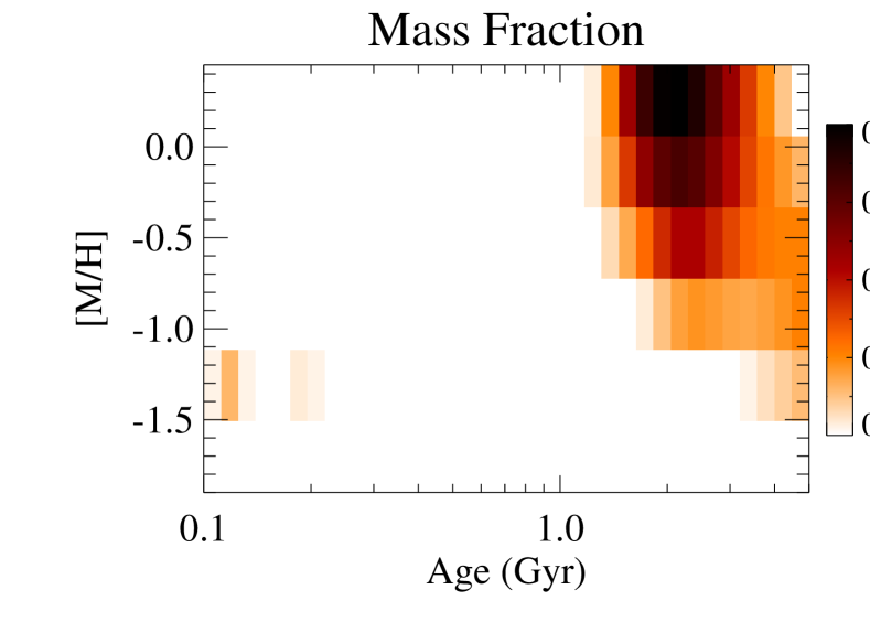
Figure 20.— The age and metallicity distribution obtained from the spectral fitting to the composite spectrum with pPXF (Cappellari & Emsellem, 2004). The colors indicate the mass fraction in each age and metallicity bin.

7. Structural and Kinematical Parameters

A puzzling property of high-redshift PEGs has emerged in recent years and is currently much debated in the literature. Indeed, several of them appear to have effective radii $\sim 2$–$5$ smaller compared to local ellipticals of the same stellar mass (e.g., Daddi et al., 2005; Trujillo et al., 2007; Cimatti et al., 2008; van Dokkum et al., 2008; Saracco et al., 2009; Cassata et al., 2011), which implies densities within their respective effective radius that are $\sim 10-100$ times higher than that to their counterparts at $z=0$. No general consensus has yet emerged about the physical mechanisms that would cause such observed size evolution, although accretion of an extended envelope via minor mergers is one widely-proposed scenario. On the other hand, $z>1.4$ PEGs with size comparable to that of local ellipticals do also exist (Mancini et al., 2010; Saracco et al., 2010), indicating that galaxies with a diversity of structural properties co-exists at these high redshifts. Possible biases that could lead to size underestimates have also been discussed (e.g., Daddi et al., 2005; Hopkins et al., 2009; Mancini et al., 2010), but it is understood that observational biases could account for only part of the effect. An independent way to check this issues is by measuring the stellar velocity dispersion ($\sigma_{*}$) from absorption lines. If they are truly compact and highly dense, their $\sigma_{*}$ should be higher than that of local ellipticals. So far $\sigma_{*}$ has been measured for only 5 or 6 individual PEGs at $z>1.4$ (Cappellari et al., 2009; Cenarro & Trujillo, 2009; van Dokkum et al., 2009; Newman et al., 2010; Onodera et al., 2010; van de Sande et al., 2011), and with one exception (van Dokkum et al., 2009) they appear structurally and dynamically similar to local ellipticals.

The structural parameters of the galaxies in the present sample are then presented and discussed in this section. We attempted the extraction of the velocity dispersion with pPXF for all galaxies. However, due to (i) the low S/N, combined with (ii) the presence of systematic sky residuals, and (iii) the low spectral resolution, a reliable results could be obtained only for the galaxy with the highest S/N.

7.1. Surface Brightness Fits and Measurement of Galaxy Sizes

We have measured the structural properties of these galaxies by fitting the 2D Sérsic profile with GALFIT version 3.0 (Peng et al., 2002, 2010a) on the HST/ACS i-band (F814W) mosaic version 2.0 over the COSMOS field which has a reduced pixel scale of 0.03 arcsec pix^-1 (Koekemoer et al., 2007; Massey et al., 2010), obtained from the original images with the MultiDrizzle routine (Koekemoer et al., 2002). The structural properties of three of these 18 galaxies (namely 254025, 307881, and 217431) have already been measured by Mancini et al. (2010) on the previous COSMOS HST/ACS release which used the original ACS pixel scale of 0.05 arcsec pix^-1. This difference has slightly affected the GALFIT results (see the next section). Here we have paid special attention to the treatment of neighboring objects, such as in object 254025 which has one bright and two faint neighbors. Therefore, in this and similar cases we used the segmentation map generated by SExtractor (Bertin & Arnouts, 1996) to mask out the faint neighbors and fit the brightest ones together with the main object.

For each galaxy, we constructed the PSF by combining unsaturated stars in the field as close as possible to each target, though using the single nearest star does not change the result at all. Indeed, the Sérsic index $n$ and effective radius $r_{\text{e}}$ vary on average within 2% of the values reported in Table 5. Some of the objects are not bright enough in the i-band (e.g., $\mathit{i}_{\text{AB}}>24$) to allow a robust estimate of the structural parameters, though we have carried out the measurement for the whole sample.

The level of the sky background is the most crucial parameter which affects the estimates of $r_{\text{e}}$ and the Sérsic index whereas the estimate of the $i$-band magnitude, position angle, and axial ratio are less affected by the adopted sky level. To account for the effect of the sky background, we ran GALFIT with different assumptions for the sky value: (i) sky as free parameter in the fit, (ii) sky fixed to the so-called “pedestal” GALFIT estimate, and (iii) sky manually measured from empty regions near the main object. By combining the results from such GALFIT runs, we derived $r_{\text{e}}$, $n$, i-band magnitude, and axial ratio as the mid point between their maximum and minimum values and quoted half such range as the corresponding error. This method provides a more reliable estimate of the actual uncertainties of these measurements compared to the small formal GALFIT errors from the $\chi^{2}$ test.

Four of the 18 galaxies (namely, 250093, 275414, 277491, and 313880) are better fit with a pure exponential profile rather than a Sérsic profile with $n>1$. For these objects the normal GALFIT fit did not converge when leaving $n$ as a free parameter, whereas an acceptable fit can be achieved when $n$ is fixed to unity. The resulting structural parameters are reported in Table 5, where effective radii are circularized (i.e., $r_{\text{e}}=a_{\text{e}}\sqrt{b/a}$ where $a_{\text{e}}$ is the effective semi-major axis as given by GALFIT and $b/a$ is the axis ratio). The disk scale lengths for the objects best-fit with the exponential profile are translated into effective radii by multiplying by 1.678.

Concerning the three galaxies included in the Mancini et al. (2010) sample, we note that the $r_{\text{e}}$ values reported in their Table 1 and Figure 4 do not refer to the circularized effective radii, but still to the effective semi-major axes $a_{\text{e}}$. Like for the other PEGs, here we use properly circularized effective radii for objects 307881, 254025, and 217431, using $b/a=0.58$, $0.65$, and $0.50$, respectively (Mancini et al. Erratum in preparation). We conclude that the radius of 307881 is in good agreement (within 10% and $1\sigma$) with the value reported in Mancini et al. (2010). Instead, the effective radii of 254025, and 217431 are $\sim 30\%$, and $\sim 45\%$ smaller, respectively, than derived in Mancini et al. (2010), though still within $\sim 1.5\sigma$ of the previous value given the large errors on $r_{\text{e}}$. The Sérsic indices are all in agreement within $\sim 20\%$ (and within $\sim 1$–$1.5\sigma$), and the other free parameters of the fit (i.e., magnitude, position angle, and axial ratio) are fully consistent (within $2$–$6$%, and $1\sigma$) within the published values. All these differences can be traced back to the different pixel size (hence PSF sampling) of the new data and to the different methods of estimating the sky background.

Table 5Structural Properties

ID	$r_{\text{e}}$		Sérsic $n$	$i_{814}$
	(arcsec)	(kpc)		(mag)
(1)	(2)	(3)	(4)	(5)
254025	$\phantom{0}0.375\pm\phantom{0}0.072$	$3.16\pm 0.61$	$3.36\pm 0.42$	$22.83\pm 0.13$
217431	$\phantom{0}0.851\pm\phantom{0}0.231$	$7.19\pm 1.95$	$3.83\pm 0.56$	$22.38\pm 0.18$
307881	$\phantom{0}0.318\pm\phantom{0}0.014$	$2.68\pm 0.12$	$2.29\pm 0.10$	$22.92\pm 0.04$
233838	$\phantom{0}0.266\pm\phantom{0}0.037$	$2.25\pm 0.31$	$3.07\pm 0.34$	$23.74\pm 0.09$
277491	$\phantom{0}0.292\pm\phantom{0}0.013$	$2.46\pm 0.11$	$1.00$	$24.31\pm 0.05$
313880	$\phantom{0}0.460\pm\phantom{0}0.063$	$3.89\pm 0.53$	$1.00$	$23.53\pm 0.19$
250093	$\phantom{0}0.356\pm\phantom{0}0.018$	$3.00\pm 0.15$	$1.00$	$24.33\pm 0.05$
263508	$\phantom{0}0.101\pm\phantom{0}0.004$	$0.86\pm 0.03$	$3.23\pm 0.21$	$23.76\pm 0.03$
269286	$\phantom{0}0.122\pm\phantom{0}0.014$	$1.03\pm 0.12$	$4.96\pm 0.72$	$23.82\pm 0.06$
240892	$\phantom{0}0.153\pm\phantom{0}0.016$	$1.29\pm 0.13$	$3.01\pm 0.34$	$24.24\pm 0.07$
205612	$\phantom{0}0.245\pm\phantom{0}0.033$	$2.08\pm 0.28$	$2.36\pm 0.26$	$24.17\pm 0.11$
251833	$\phantom{0}0.190\pm\phantom{0}0.011$	$1.61\pm 0.09$	$2.13\pm 0.13$	$24.01\pm 0.04$
228121	$\phantom{0}0.329\pm\phantom{0}0.102$	$2.78\pm 0.86$	$4.07\pm 0.89$	$24.40\pm 0.20$
321998	$\phantom{0}0.216\pm\phantom{0}0.040$	$1.83\pm 0.34$	$4.40\pm 0.65$	$24.15\pm 0.10$
299038	$\phantom{0}0.114\pm\phantom{0}0.002$	$0.96\pm 0.02$	$1.89\pm 0.05$	$24.94\pm 0.02$
209501	$\phantom{0}0.077\pm\phantom{0}0.000$	$0.65\pm 0.00$	$1.63\pm 0.01$	$24.97\pm 0.00$
253431	$\phantom{0}0.317\pm\phantom{0}0.022$	$2.69\pm 0.18$	$4.23\pm 0.19$	$24.46\pm 0.04$
275414	$\phantom{0}0.269\pm\phantom{0}0.015$	$2.27\pm 0.13$	$1.00$	$25.07\pm 0.05$

Note. — (1) ID; (2) effective radius in arcseconds; (3) effective radius in kpc; (4) Sérsic index; (5) HST/ACS $i$-band magnitude recovered by GALFIT. The effective radii are circularized and the disk scale lengths for the objects best fitted with the exponential profile are converted into effective radii.

7.2. Stellar mass–size relation

Figure 21 shows the resulting effective radii of the program galaxies as a function of the stellar mass. For comparison, the local relation derived by Newman et al. (2012) is also shown, together with the subset of $z>1.4$ PEGs from the compilation of 465 PEGs with spectroscopic redshift by Damjanov et al. (2011). For both data sets we have converted the stellar masses into those appropriate for the Chabrier IMF by using correction factors shown in Table 2 of Bernardi et al. (2010). The majority of these galaxies appear to be more compact compared to local PEGs of the same mass, although about a third of them lies on, or close to, the local relation (within $\sim 2\sigma$), whereas 7 of them (i.e., $\sim 40$%) are more than $3\sigma$ from the local relation. When only the brighter objects with $\mathit{i}<24$ are considered, then $\sim 50$% are classified as compact.

Note that the sizes of high-$n$ galaxies, in particular the fainter ones, may have been systematically underestimated as shown by simulations (Mancini et al., 2010), an effect that may not be confined only to high redshift galaxies. For example, the measured effective radius of M87 can vary by up to a factor of two, depending on the depth of the adopted photometry (Kormendy et al., 2009). These uncertainties may well affect the derived fractions of normal and compact objects in our sample.

Figure 22 shows the effective radius of the 18 galaxies (normalized to the local relation) vs. their spectroscopic redshift, along with the objects in the compilation of Damjanov et al. (2011). About 40% of our sample show $r_{\text{e}}/r_{\text{e},z=0}<0.3$ while previous studies have found a slightly stronger evolution with $\gtrsim 50\%$ of PEGs at $z\simeq 1.6$ with $M\gtrsim 10^{11}\,M_{\odot}$ having $r_{\text{e}}/r_{\text{e},z=0}\lesssim 0.3$ (e.g., Trujillo et al., 2007; Buitrago et al., 2008; Damjanov et al., 2011; Newman et al., 2012). Cooper et al. (2012) have shown that PEGs at $0.4<z<1.2$ in high density regions tend to be bigger by up to $\sim 25\%$ than those in low density regions. If this trend were to continue towards higher redshifts then the present PEG sample may be slightly biased towards larger sizes compared to those in the general field, as our galaxies are preferentially located in overdense regions (see Section 4).

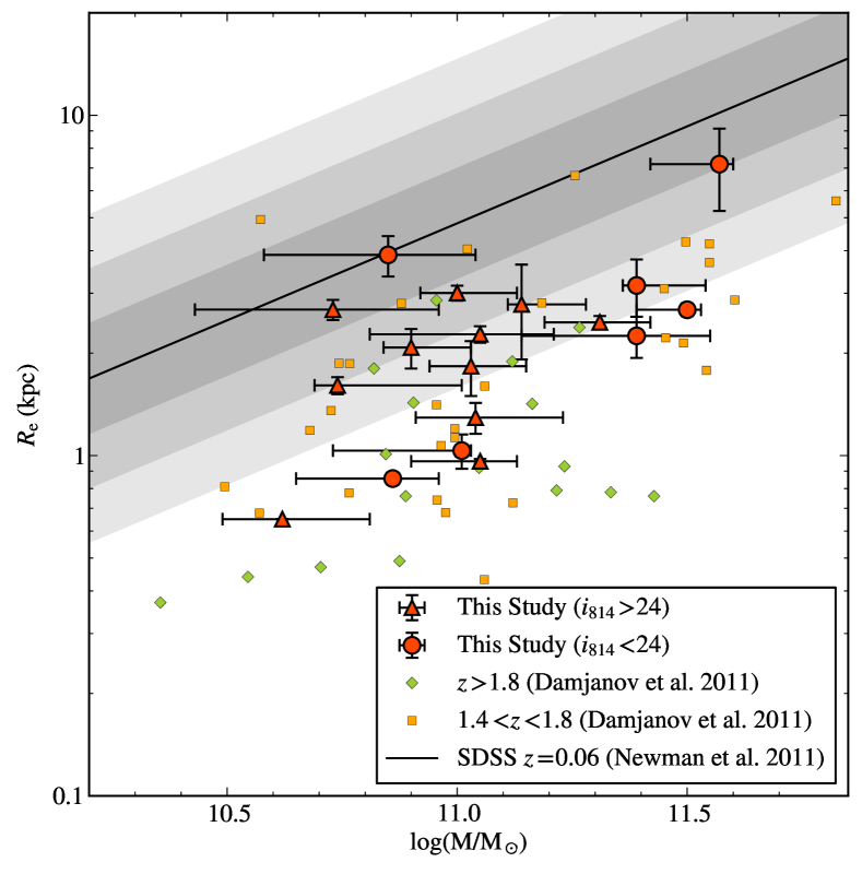
Figure 21.— The stellar mass–size relation of our spectroscopically identified pBzKs at $1.4\lesssim z\lesssim 1.8$ with $\mathit{i}_{814}<24$ (red circles) and $\mathit{i}_{814}>24$ (red triangles), where $\mathit{i}_{814}$ is the HST/ACS F814W magnitude recovered by GALFIT. The orange squares and green diamonds represent passively evolving galaxies from the compilation of Damjanov et al. (2011) with spectroscopic redshifts respectively in the range $1.4<z<1.8$ (the same as in our study) and at $z>1.8$. The solid line refers to the mean mass–size relation for $z=0.06$ passive galaxies in SDSS from Newman et al. (2012) and the gray shaded bands show the $1\sigma$, $2\sigma$ and $3\sigma$ deviations from such relation.

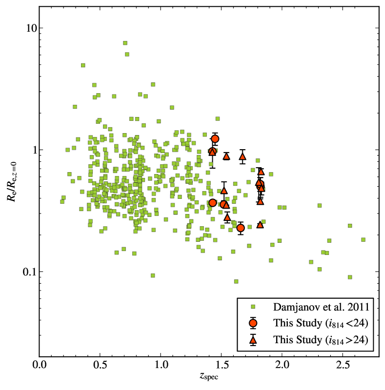
Figure 22.— The effective radii of the pBzKs presented here (circles) and those of the passive galaxies with spectroscopic redshift from Damjanov et al. (2011), normalized to the mass–size relation at $z=0.06$ from Newman et al. (2012) at the same stellar mass.

7.3. Relation between Size and Age Indicators

One effect contributing to the evolution of the mass–size relation of PEGs comes from the progressive quenching of larger star-forming galaxies (van der Wel et al., 2009; Valentinuzzi et al., 2010; Cassata et al., 2011). In this scenario, one expect that younger, i.e., recently quenched, PEGs have size close to the local relation, while older ones, i.e., quenched at an earlier time, are more compact. If so, one would expect some correlation between the SED-derived age and a departure from the local mass-size relation. Based on the SED ages of 62 spectroscopically identified PEGs at $0.9<z<2$, Saracco et al. (2011) claimed that the normal size high-$z$ elliptical galaxies have relatively younger stellar population ages compared to the compact ones that would show a wider range of formation redshifts with a large fraction of them having formed at $z>5$. In contrast, Whitaker et al. (2012) found that younger PEGs at $1.5<z<2.0$ are more centrally concentrated and may have slightly smaller sizes. To check for this effect in our sample, we have compared the size and age indicators, namely ages from broad-band SED fitting and Dn4000 indices.

The left panel of Figure 23 compares the size normalized to the local mass-size relation with the age from the SED fitting. Besides the present pBzK sample, the SED ages of spectroscopically identified PEGs at similar redshifts from Cimatti et al. (2008) and Saracco et al. (2011) are also shown for comparison. As pointed out by Saracco et al. (2011), in their data there appears to be a weak trend with compact galaxies showing a wider range of SED ages compared to normal-size ones that tend to show younger ages. Splitting our sample at $\log(r_{\text{e}}/r_{\text{e},z=0})=-0.48$ ($3\sigma$ deviation from the local mass–size relation), the median of $\log(\text{Age/yr})$ are 9.15 and 9.40 for the normal and compact galaxies, respectively, i.e., the compact galaxies appear to be $\sim 70\%$ (or about 1 Gyr) older than the normal ones. When only the objects with $\mathit{i}_{814}<24$ are considered, the median $\log(\text{Age/yr})$ are 9.10 and 9.35 for normal and compact objects, respectively. Note that the uncertainties in the SED ages are typically comparable to these differences.

The right panel of Figure 23 shows the relation between the normalized size and Dn4000, which can be taken as a proxy for stellar population age. For comparison, a compact quenched galaxy at $z=2.2$ (Kriek et al., 2009) is also shown. Excluding the object with exceptionally large Dn4000 ($\sim 2.75$), there seems to be essentially no trend between size and Dn4000. The median Dn4000 of the normal and compact objects are 1.61 and 1.55, respectively, a difference comparable to the typical $1\sigma$ error in Dn4000 measurement. Restricting the sample to the brightest objects, the median Dn4000 of normal and compact objects are 1.42 and 1.50, respectively.

We conclude that in our sample there is no strong correlation between the size of high redshift PEGs and stellar population age. A Similar conclusion is also found for the brightest objects for which the size measurements are more reliable. To draw any firm conclusions it is essential to construct a larger sample with robustly measured size and Dn4000.

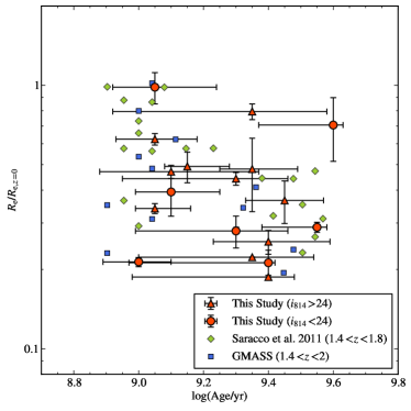
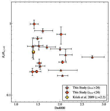
Figure 23.— Left: The effective radius of passively evolving galaxies with spectroscopic redshifts at $z>1.4$ as a function of their stellar population age from SED fitting. Red circles and triangles, green diamonds, and blue squares represent the pBzK sample in our study (depending on their F814W magnitude as in Figure 21), the passively evolving galaxies studied by Saracco et al. (2011) at $1.4<z<1.8$, and those from the GMASS survey (Cimatti et al., 2008) at $1.4<z<2$. Right: Same as the left panel, but expressed as a function of Dn4000. Red symbols are the same as in the left panel, and a yellow square represents a galaxy at $z=2.2$ from Kriek et al. (2009).

7.4. Stellar Velocity Dispersion of the pBzK Galaxy 254025

For the brightest object in the sample (254025) a $1\sigma$ upper limit to its stellar velocity dispersion ($\sigma_{*}<304$ $\,\text{km}~{}\text{s}^{-1}$) was placed by Onodera et al. (2010) based on our MOIRCS 2009 data. By adding the data taken in 2010 we have been able to upgrade this upper limit to a true measurement of $\sigma_{*}$. We used a FWHM of 27 Å at the observed wavelength for the instrumental profile and assumed the resolution to be constant in linear wavelength scale across the wavelength range of interest. We have restricted the analysis to the $3550$–$4450$ Å rest frame wavelength range with $\text{S/N}=11.5$ in 60 km s^-1 spectral interval, which encompasses features such as CN, Ca II H&K, H$\delta$, the G band, H$\gamma$ and Fe 4383. We determined a dispersion $\sigma_{*}=270\pm 105$ $\,\text{km}~{}\text{s}^{-1}$ from 300 realizations of pPXF fits that consider not only the effect of random noise, but also explore the effect of sky residuals and different input parameters in pPXF, as described in Section 3.1. Here for $\sigma_{*}$ we take the median of the distribution and the $1\sigma$ error is determined as $(\sigma_{*,84}-\sigma_{*,16})/2$ where $\sigma_{*,84}$ and $\sigma_{*,16}$ correspond respectively to the 84- and 16-percentiles of the probability distribution. We emphasize that the quoted error is very conservative, as a formal random error of only 32 $\,\text{km}~{}\text{s}^{-1}$ is indicated by single pPXF fits. We quote instead an error of 105 $\,\text{km}~{}\text{s}^{-1}$ derived above as a more realistic value that includes an estimate of the systematic errors.

Figure 24 compares the structural and dynamical properties of the galaxy 254025 with those of local early type galaxies and with those from the small sample of $z>1$ PEGs for which a stellar velocity dispersion has been measured. Dynamical masses are derived as $M_{\text{dyn}}=5r_{\text{e}}\sigma_{*}^{2}/G$ where $G$ is the gravitational constant, and we obtained $\log(M_{\text{dyn}}/M_{\odot})=11.43\pm 0.35$ for the galaxy 254025. Figure 24 is an update of the similar figure presented in Onodera et al. (2010). We can thus confirm that this galaxy closely follows all the local relations involving the dynamical mass, the effective radius and the stellar velocity dispersion within the error bars. Again, this is a proof of the coexistence at high redshifts of PEGs that appear structurally and dynamically similar to their local counterparts with other galaxies that are more compact and are correspondingly characterized by a higher velocity dispersion.

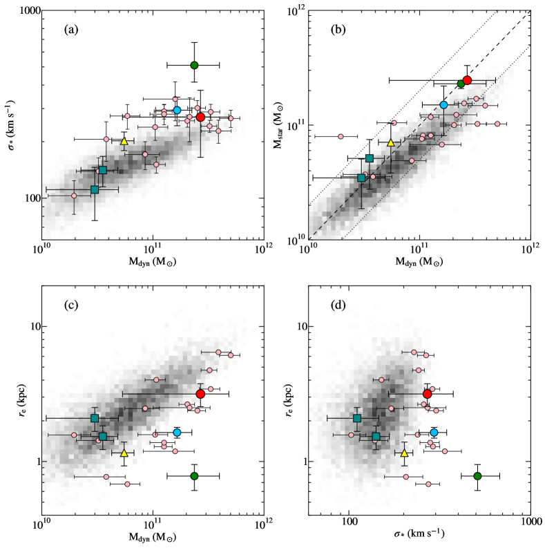
Figure 24.— A comparison of the structural/dynamical properties of high-redshift early-type galaxies with measured velocity dispersions (symbols with error bars) with those from SDSS elliptical galaxies at $z\simeq 0.06$ (shown as gray scale). (a): The stellar velocity dispersions vs. the dynamical mass. (b): Comparison between the dynamical and the stellar masses; the diagonal dashed line refers to equal mass and the dotted lines show the range around it by a factor of 2. (c): The effective radii vs. the dynamical masses. (d): The effective radii vs. the stellar velocity dispersions. In all panels, the symbols refer to: the galaxy 254025 from the present study (red filled circle); an object at $z=2.19$ (green filled circle; van Dokkum et al., 2009); two GMASS galaxies at $z=1.41$ and the stacked properties of the GMASS galaxies at $1.6<z<2.0$ (blue squares and yellow triangle, respectively; Cappellari et al., 2009); an object at $z=1.80$ (cyan circle; van de Sande et al., 2011); and objects at $1.05<z<1.60$ (small pink circles; Newman et al., 2010).

8. Number and Stellar Mass Densities

As our spectroscopic identification of the PEGs with $K<21$ or $M_{*}\gtrsim 10^{11}\,M_{\odot}$ is nearly complete over the surveyed area, we can estimate the abundance of massive PEGs at $z>1.4$, to within cosmic variance errors. The redshift range covered by the present sample $1.43\lesssim z\lesssim 1.83$ over the survey area of 66.2 arcmin² contains a comoving volume of $\sim 82,000$ Mpc³. Thus, from the 16 objects with $K<21$ we estimate a comoving number density of $1.9\times 10^{-4}$ Mpc^-3, and the corresponding stellar mass density is $3.0\times 10^{7}\,M_{\odot}$ Mpc^-3, with an uncertainty of $\sim 25\%{}$ from Poisson statistics. These should be regarded as upper limits since the field was chosen for its overdensity of PEGs. However they are in agreement with estimates derived from a complete sample of galaxies in the Hubble Ultra Deep Field of $3.4\times 10^{-4}$ Mpc^-3 and $1.9$–$4.6\times 10^{7}\,M_{\odot}$ Mpc^-3 (after converting to Chabrier IMF), as measured by Daddi et al. (2005) for spectroscopically identified PEGs at $1.39<z<2.00$ down to the limit $K=23$, although their explored comoving volume is $\sim 4$ times smaller.

Brammer et al. (2011) have derived number and mass densities of PEGs at $0.4<z_{\rm phot}<2.2$ from the NEWFIRM Medium Band Survey (NMBS), covering an area of $\sim 0.4$ deg², and for the mean redshift of our galaxies ($z=1.69$) found $(1.0\pm 0.3)\times 10^{-4}$ Mpc^-3 and $(1.6\pm 0.4)\times 10^{7}\,M_{\odot}$ Mpc^-3, respectively. Our estimates are somewhat higher, as expected given the mentioned overdensity bias.

Comparing to the corresponding local values, respectively $\sim 4\times 10^{-4}$ Mpc^-3 and $\sim 8\times 10^{7}\,M_{\odot}$ Mpc^-3 from Baldry et al. (2004), taken at face value our result suggests that PEGs at $1.4\lesssim z\lesssim 1.8$ account for $\sim 50\%$ of the number density and $\sim 35$–$40\%$ of the stellar mass density of local PEGs with $M_{*}>10^{11}\,M_{\odot}$.

9. Summary and Conclusions

Mapping the 3D space distribution of passively evolving galaxies at high redshift is an endeavour of critical importance in the broader context of galaxy evolution and observational cosmology. However, it is perhaps also the most challenging observationally, as it requires many hundreds of hours of 8m-class telescope time with current instrumentation. Emission lines are absent (or very weak) in the spectra of PEGs, and therefore measuring redshifts and velocity dispersions must rely uniquely on absorption lines. With spectrometers working at optical wavelengths, for such objects at $z\gtrsim 1.4$ this is possible using absorption lines over an intrinsically very faint UV continuum, which requires extremely long integration times. Using near-IR, multiobject spectrometers offers a potentially attractive alternative, as the strongest spectral features over a strong continuum become accessible. However, ground based, infrared spectroscopy of faint, high redshift objects is affected by a higher sky and thermal background which largely limits this advantage. Using the MOIRCS instrument at the Subaru telescope we have started a pilot experiment aimed at studying a sample of bright PEGs at $z\gtrsim 1.4$ while assessing the feasibility of a more ambitious project.

With this objective, we have first identified the strongest concentrations of high-$z$ candidate PEGs over the COSMOS field, and focused our observational effort over one such concentration and its immediate vicinity. A sample of 34 objects has been observed, with integration times ranging from 280 to 550 minutes, and the continuum has been detected in 18 of them. The redshift of these detected galaxies are concentrated in three spikes at $z=1.43$, 1.53 and 1.82, and the last two galaxies have quite similar redshifts around 1.67. This spectroscopically confirms the strong clustering of high redshift PEGs, previously hinted only from their 2-point correlation function (e.g., Kong et al., 2006; McCracken et al., 2010). A comparison with COSMOS photometric redshifts shows that $\sim 2/3$ of them agree closely with the spectroscopic redshifts, whereas the other $\sim 1/3$ of them are systematically underestimated by up to $\sim 25\%$. Thus, these photometric redshifts can lead to a sizable underestimate of the volume density of PEGs at $z\gtrsim 1.4$. However, we show that photometric redshift training with these spectroscopic redshifts can significantly improve their performance for high-$z$ PEGs.

Having fixed the redshifts to their spectroscopic values, we have explored the stellar population content of these galaxies, measuring their masses, luminosity-weighted ages and metallicities using various SED-fitting techniques. Stellar masses range from $\sim 4\times 10^{10}$ to $\sim 4\times 10^{11}\,M_{\odot}$, ages from $\sim 1$ to $\sim 3$ Gyr, whereas near-solar metallicity is found for most galaxies.

The Lick H$\delta_{\text{F}}$ and the Dn4000 indices allowed us to investigate further the stellar population content and evolutionary stage of the sample galaxies. We find that about 40% of the pBzKs show large Dn4000 (around 2) which indicates that these galaxies are already quenched long ago compared to their timescale of star formation. On the other hand, about 60% of them have Dn4000 values close to those of young star-forming or post-starburst galaxies, which indicates that these galaxies have been quenched more recently, given the lack of the star-forming activity (except for one object with a mid-IR detection). This is also confirmed for the four most massive and brightest objects and the composite spectrum with measurable H$\delta$ absorption line. Two of them (as well as the composite spectrum, see below) show moderate Dn4000 and H$\delta_{\text{F}}$, consistent with the early stages of a post-starburst galaxy where star formation has been quenched very recently. The other two bright galaxies show both large Dn4000 and H$\delta_{\text{F}}$ and appear to be already passive, possibly with a recent episode of star-formation, though the combination of two indices seems rather extreme.

The composite spectrum of the 17 galaxies exhibits several well-detected spectral features, notably CN, Ca II H&K, the G band, H$\beta,\gamma,\delta$, Mg$b$ and various iron lines. A fit to this composite spectrum indicates that it is dominated by old, metal-rich stellar populations with a mass-weighted age of $\sim 3.5$ Gyr. The fit is somewhat dependent on the allowed age and metallicity ranges, but the existence of stellar population younger than $\sim 400$ Myr is always excluded by the fits, which is confirmed by the use of another fitting code adopting a different input SSP library.

The structural parameters, (circularized) effective radius and Sérsic index, have been measured for these galaxies over the HST/ACS i-band image of the COSMOS field. A majority of the 18 galaxies have effective radii somewhat lower than equally massive galaxies in the local Universe, with some up to three times lower. However, almost about a third of the galaxies appear to be on, or close to, the local $r_{\text{e}}-M_{*}$ relation, confirming that compact and apparently normal PEGs coexist at these redshifts.

Finally, the stellar velocity dispersion of the brightest galaxy in the sample was measured as $\sigma_{*}=270\pm 105$ $\,\text{km}~{}\text{s}^{-1}$. Combined with its effective radius and stellar mass, this value of $\sigma_{*}$ confirms that this $z=1.82$ galaxy closely follows all the local structural and dynamical relations for PEGs.

The nearly complete identification of PEGs at the top end of their stellar mass function at the observed redshift range allows us to estimate their number and stellar mass densities, still with the proviso that they refer to an overdensity region. Thus, the PEGs with $M*\gtrsim 10^{11}\,M_{\odot}$ at $1.4\gtrsim z\gtrsim 1.8$ we found in the studied field correspond to about 50% of the number and about 35–40% of the stellar mass densities of local PEGs with similar stellar mass.

Without counting the time lost to technical problems and bad weather, this project has used 4–5 nights of Subaru telescope time. Over the whole 2 square degree COSMOS field one can roughly count $\sim 20$ concentrations of candidate high-$z$ PEGs similar to the one explored in the present study. Thus, some 80–100 nights would be required to map all such concentrations in a similar fashion with Subaru/MOIRCS. Obviously, even more would be required to map the distribution of all massive PEGs over the entire COSMOS field. A coordinated effort with the upcoming near-IR multi-object spectrographs at 8–10 m class telescopes (such as Gemini/FLAMINGOS-II, VLT/KMOS, and Keck/MOSFIRE) would be required to make such large project feasible in the near future.

References

- Baldry et al. (2004) Baldry, I. K., Glazebrook, K., Brinkmann, J., Ivezić, Ž., Lupton, R. H., Nichol, R. C., & Szalay, A. S. 2004, ApJ, 600, 681
- Balogh et al. (1999) Balogh, M. L., Morris, S. L., Yee, H. K. C., Carlberg, R. G., & Ellingson, E. 1999, ApJ, 527, 54
- Bernardi et al. (2010) Bernardi, M., Shankar, F., Hyde, J. B., Mei, S., Marulli, F., & Sheth, R. K. 2010, MNRAS, 404, 2087
- Bertin & Arnouts (1996) Bertin, E., & Arnouts, S. 1996, A&AS, 117, 393
- Blanton et al. (2005) Blanton, M. R., et al. 2005, AJ, 129, 2562
- Bolzonella et al. (2010) Bolzonella, M., et al. 2010, A&A, 524, A76
- Brammer et al. (2008) Brammer, G. B., van Dokkum, P. G., & Coppi, P. 2008, ApJ, 686, 1503
- Brammer et al. (2009) Brammer, G. B., et al. 2009, ApJ, 706, L173
- Brammer et al. (2011) —. 2011, ApJ, 739, 24
- Bruzual & Charlot (2003) Bruzual, G., & Charlot, S. 2003, MNRAS, 344, 1000
- Buitrago et al. (2008) Buitrago, F., Trujillo, I., Conselice, C. J., Bouwens, R. J., Dickinson, M., & Yan, H. 2008, ApJ, 687, L61
- Calzetti et al. (2000) Calzetti, D., Armus, L., Bohlin, R. C., Kinney, A. L., Koornneef, J., & Storchi-Bergmann, T. 2000, ApJ, 533, 682
- Cappellari & Emsellem (2004) Cappellari, M., & Emsellem, E. 2004, PASP, 116, 138
- Cappellari et al. (2009) Cappellari, M., et al. 2009, ApJ, 704, L34
- Cappellari et al. (2012) —. 2012, Nature, 484, 485
- Cassata et al. (2011) Cassata, P., et al. 2011, ApJ, 743, 96
- Cenarro & Trujillo (2009) Cenarro, A. J., & Trujillo, I. 2009, ApJ, 696, L43
- Chabrier (2003) Chabrier, G. 2003, PASP, 115, 763
- Chary & Elbaz (2001) Chary, R., & Elbaz, D. 2001, ApJ, 556, 562
- Cid Fernandes et al. (2005) Cid Fernandes, R., Mateus, A., Sodré, L., Stasińska, G., & Gomes, J. M. 2005, MNRAS, 358, 363
- Cid Fernandes et al. (2009) Cid Fernandes, R., et al. 2009, in Revista Mexicana de Astronomia y Astrofisica Conference Series, Vol. 35, Revista Mexicana de Astronomia y Astrofisica Conference Series, 127–132
- Cimatti et al. (2006) Cimatti, A., Daddi, E., & Renzini, A. 2006, A&A, 453, L29
- Cimatti et al. (2004) Cimatti, A., et al. 2004, Nature, 430, 184
- Cimatti et al. (2008) —. 2008, A&A, 482, 21
- Cooper et al. (2012) Cooper, M. C., et al. 2012, MNRAS, 419, 3018
- Daddi et al. (2004) Daddi, E., Cimatti, A., Renzini, A., Fontana, A., Mignoli, M., Pozzetti, L., Tozzi, P., & Zamorani, G. 2004, ApJ, 617, 746
- Daddi et al. (2005) Daddi, E., et al. 2005, ApJ, 626, 680
- Daddi et al. (2007) —. 2007, ApJ, 670, 156
- Damjanov et al. (2011) Damjanov, I., et al. 2011, ApJ, 739, L44
- Falcón-Barroso et al. (2011) Falcón-Barroso, J., Sánchez-Blázquez, P., Vazdekis, A., Ricciardelli, E., Cardiel, N., Cenarro, A. J., Gorgas, J., & Peletier, R. F. 2011, A&A, 532, A95
- Finoguenov et al. (2007) Finoguenov, A., et al. 2007, ApJS, 172, 182
- Förster Schreiber et al. (2011) Förster Schreiber, N. M., et al. 2011, ApJ, 739, 45
- Genzel et al. (2011) Genzel, R., et al. 2011, ApJ, 733, 101
- Graves & Schiavon (2008) Graves, G. J., & Schiavon, R. P. 2008, ApJS, 177, 446
- Hasinger et al. (2007) Hasinger, G., et al. 2007, ApJS, 172, 29
- Hoaglin et al. (1983) Hoaglin, D. C., Mosteller, F., & Tukey, J. W. 1983, Understanding robust and exploratory data anlysis, ed. Hoaglin, D. C., Mosteller, F., & Tukey, J. W.
- Hopkins et al. (2009) Hopkins, P. F., Bundy, K., Murray, N., Quataert, E., Lauer, T. R., & Ma, C.-P. 2009, MNRAS, 398, 898
- Ichikawa et al. (2006) Ichikawa, T., et al. 2006, in Society of Photo-Optical Instrumentation Engineers (SPIE) Conference Series, Vol. 6269, Society of Photo-Optical Instrumentation Engineers (SPIE) Conference Series
- Ilbert et al. (2009) Ilbert, O., et al. 2009, ApJ, 690, 1236
- Ilbert et al. (2010) —. 2010, ApJ, 709, 644
- Kauffmann et al. (2003) Kauffmann, G., et al. 2003, MNRAS, 341, 33
- Koekemoer et al. (2002) Koekemoer, A. M., Fruchter, A. S., Hook, R. N., & Hack, W. 2002, in The 2002 HST Calibration Workshop : Hubble after the Installation of the ACS and the NICMOS Cooling System, ed. S. Arribas, A. Koekemoer, & B. Whitmore (Baltimore, MD: STScI), 337, ed. S. Arribas, A. Koekemoer, & B. Whitmore, 337
- Koekemoer et al. (2007) Koekemoer, A. M., et al. 2007, ApJS, 172, 196
- Kong et al. (2006) Kong, X., et al. 2006, ApJ, 638, 72
- Kormendy et al. (2009) Kormendy, J., Fisher, D. B., Cornell, M. E., & Bender, R. 2009, ApJS, 182, 216
- Kriek et al. (2009) Kriek, M., van Dokkum, P. G., Labbé, I., Franx, M., Illingworth, G. D., Marchesini, D., & Quadri, R. F. 2009, ApJ, 700, 221
- Kriek et al. (2006) Kriek, M., et al. 2006, ApJ, 649, L71
- Kriek et al. (2008) —. 2008, ApJ, 677, 219
- Kroupa (2001) Kroupa, P. 2001, MNRAS, 322, 231
- Le Borgne et al. (2006) Le Borgne, D., et al. 2006, ApJ, 642, 48
- Le Floc’h et al. (2009) Le Floc’h, E., et al. 2009, ApJ, 703, 222
- Lilly et al. (2007) Lilly, S. J., et al. 2007, ApJS, 172, 70
- Lilly et al. (2009) —. 2009, ApJS, 184, 218
- Maíz Apellániz (2006) Maíz Apellániz, J. 2006, AJ, 131, 1184
- Mancini et al. (2010) Mancini, C., et al. 2010, MNRAS, 401, 933
- Mancini et al. (2011) —. 2011, ApJ, 743, 86
- Maraston (2005) Maraston, C. 2005, MNRAS, 362, 799
- Maraston et al. (2010) Maraston, C., Pforr, J., Renzini, A., Daddi, E., Dickinson, M., Cimatti, A., & Tonini, C. 2010, MNRAS, 407, 830
- Massey et al. (2010) Massey, R., Stoughton, C., Leauthaud, A., Rhodes, J., Koekemoer, A., Ellis, R., & Shaghoulian, E. 2010, MNRAS, 401, 371
- McCarthy et al. (2004) McCarthy, P. J., et al. 2004, ApJ, 614, L9
- McCracken et al. (2010) McCracken, H. J., et al. 2010, ApJ, 708, 202
- Newman et al. (2012) Newman, A. B., Ellis, R. S., Bundy, K., & Treu, T. 2012, ApJ, 746, 162
- Newman et al. (2010) Newman, A. B., Ellis, R. S., Treu, T., & Bundy, K. 2010, ApJ, 717, L103
- Oke & Gunn (1983) Oke, J. B., & Gunn, J. E. 1983, ApJ, 266, 713
- Onodera et al. (2010) Onodera, M., et al. 2010, ApJ, 715, L6
- Pannella et al. (2009) Pannella, M., et al. 2009, ApJ, 698, L116
- Papovich et al. (2011) Papovich, C., Finkelstein, S. L., Ferguson, H. C., Lotz, J. M., & Giavalisco, M. 2011, MNRAS, 412, 1123
- Peng et al. (2002) Peng, C. Y., Ho, L. C., Impey, C. D., & Rix, H.-W. 2002, AJ, 124, 266
- Peng et al. (2010a) —. 2010a, AJ, 139, 2097
- Peng et al. (2011) Peng, Y., Lilly, S. J., Renzini, A., & Carollo, M. 2011, ArXiv e-prints
- Peng et al. (2010b) Peng, Y.-j., et al. 2010b, ApJ, 721, 193
- Pickles (1998) Pickles, A. J. 1998, PASP, 110, 863
- Pozzetti et al. (2010) Pozzetti, L., et al. 2010, A&A, 523, A13
- Press et al. (1992) Press, W. H., Teukolsky, S. A., Vetterling, W. T., & Flannery, B. P. 1992, Numerical recipes in FORTRAN. The art of scientific computing, ed. Press, W. H., Teukolsky, S. A., Vetterling, W. T., & Flannery, B. P.
- Renzini (2009) Renzini, A. 2009, MNRAS, 398, L58
- Rodighiero et al. (2011) Rodighiero, G., et al. 2011, ApJ, 739, L40
- Rousselot et al. (2000) Rousselot, P., Lidman, C., Cuby, J., Moreels, G., & Monnet, G. 2000, A&A, 354, 1134
- Salim et al. (2007) Salim, S., et al. 2007, ApJS, 173, 267
- Sánchez-Blázquez et al. (2006) Sánchez-Blázquez, P., et al. 2006, MNRAS, 371, 703
- Sanders et al. (2007) Sanders, D. B., et al. 2007, ApJS, 172, 86
- Saracco et al. (2009) Saracco, P., Longhetti, M., & Andreon, S. 2009, MNRAS, 392, 718
- Saracco et al. (2010) Saracco, P., Longhetti, M., & Gargiulo, A. 2010, MNRAS, 408, L21
- Saracco et al. (2011) —. 2011, MNRAS, 412, 2707
- Scarlata et al. (2007) Scarlata, C., et al. 2007, ApJS, 172, 494
- Schiavon (2007) Schiavon, R. P. 2007, ApJS, 171, 146
- Scoville et al. (2007) Scoville, N., et al. 2007, ApJS, 172, 1
- Suzuki et al. (2008) Suzuki, R., et al. 2008, PASJ, 60, 1347
- Taylor et al. (2009) Taylor, E. N., et al. 2009, ApJ, 694, 1171
- Trujillo et al. (2007) Trujillo, I., Conselice, C. J., Bundy, K., Cooper, M. C., Eisenhardt, P., & Ellis, R. S. 2007, MNRAS, 382, 109
- Valentinuzzi et al. (2010) Valentinuzzi, T., et al. 2010, ApJ, 721, L19
- van de Sande et al. (2011) van de Sande, J., et al. 2011, ApJ, 736, L9
- van der Wel et al. (2009) van der Wel, A., Bell, E. F., van den Bosch, F. C., Gallazzi, A., & Rix, H.-W. 2009, ApJ, 698, 1232
- van Dokkum et al. (2009) van Dokkum, P. G., Kriek, M., & Franx, M. 2009, Nature, 460, 717
- van Dokkum et al. (2008) van Dokkum, P. G., et al. 2008, ApJ, 677, L5
- Vazdekis et al. (2010) Vazdekis, A., Sánchez-Blázquez, P., Falcón-Barroso, J., Cenarro, A. J., Beasley, M. A., Cardiel, N., Gorgas, J., & Peletier, R. F. 2010, MNRAS, 404, 1639
- Vergani et al. (2010) Vergani, D., et al. 2010, A&A, 509, A42
- Whitaker et al. (2012) Whitaker, K. E., Kriek, M., van Dokkum, P. G., Bezanson, R., Brammer, G., Franx, M., & Labbé, I. 2012, ApJ, 745, 179
- Whitaker et al. (2011) Whitaker, K. E., et al. 2011, ApJ, 735, 86
- Williams et al. (2009) Williams, R. J., Quadri, R. F., Franx, M., van Dokkum, P., & Labbé, I. 2009, ApJ, 691, 1879
- Worthey et al. (1994) Worthey, G., Faber, S. M., Gonzalez, J. J., & Burstein, D. 1994, ApJS, 94, 687
- Worthey & Ottaviani (1997) Worthey, G., & Ottaviani, D. L. 1997, ApJS, 111, 377
- Wuyts et al. (2007) Wuyts, S., et al. 2007, ApJ, 655, 51
- Yoshikawa et al. (2010) Yoshikawa, T., et al. 2010, ApJ, 718, 112